On The Diffusion of Sticky Particles in 1-D

Abstract

The 1D Ising model is the simplest Hamiltonian-based model in statistical mechanics. The sim- plest interacting particle process is the Symmetric Exclusion Process (SEP), a 1D lattice gas of particles that hop symmetrically and cannot overlap. Combining the two gives a model for sticky particle diffusion, SPM, which is described here. SPM dynamics are based on SEP with short-range interaction, allowing flow due to non-equilibrium boundary conditions. We prove that SPM is also a detailed-balance respecting, particle-conserving, Monte Carlo (MC) description of the Ising model. Neither the Ising model nor SEP have a phase transition in 1D, but the SPM exhibits a non-equilibrium transition from a diffusing to a blocked state as stickiness increases. This transition manifests in peaks in the MC density fluctuation, a change in the dependency of flow-rate on stickiness, and odd structure in the eigenspectrum of the transition rate matrix. We derive and solve a fully non-linear, analytic, mean-field solution, which has a crossover from a positive to a negative diffusion constant where the MC shows the transition. The negative diffusion constant in fact indicates a breakdown of the mean-field approximation, with close to zero flow and breaking into a two-phase mixture, and thus the mean field theory successfully predicts its own demise. We also present an analytic solution for the flow via direct analysis of the transition rate matrix. The simplicity of the model suggest a wide range of possible applications.

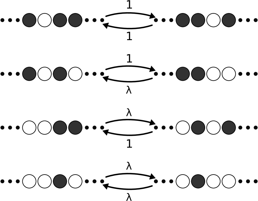
Figure 1: White circles indicate particles, dark circles indicate empty sites (vacancies). Particles randomly move into adjacent vacancies with rate $1$ (having rescaled time for notational convenience), unless there is a particle behind the position they’re moving from, in which case they move with rate $\lambda$; the state of the site next to the position the particle is moving into is irrelevant.

I Introduction

Lattice gases are a ubiquitous tool for modeling complex systems from biology to traffic Belitsky and Schütz (2011); Mobilia et al. (2007); Tegner et al. (2015); Zhu et al. (2012); Deal and Grove (1965); Cabrera and Mott (1949); Buzzaccaro et al. (2007). Analytically solvable cases involve non-interacting or excluding particles Ladd et al. (1988); Liggett (1985); Ben-Naim et al. (1999); Shandarin and Zeldovich (1989); Frachebourg (1999); Frachebourg et al. (2000), but in any real system of interest the moving objects interact. Many models tackle the situation where the diffusing objects interact with the substrate, but despite clear application-relevance there is surprisingly little work considering interactions between the moving particles themselves. One reason for this is that the interactions introduce nonlinearities in analytical models, which makes them challenging to solve, at least outside of limits in which they can be linearized. This is unfortunate because it is precisely these nonlinearities which introduce interesting behaviors such as discontinuities at interfaces or diffusion instability Obukhovsky et al. (2017); Gorokhova and Melnik (2010).

Another feature of previous models is that the flow is driven by either asymmetry in the dynamics (e.g. the Asymmetric Simple Exclusion Process, ASEP) or an external field which permeates the system (e.g. the Katz-Lebowitz-Spohn model, KLS). In either case, the particles always see a local asymmetry. However in many systems the flow is driven by a pressure or chemical potential difference applied at the boundaries, so that any local asymmetry arises from self-organization. This is the situation that is addressed here.

In this paper we will investigate what we believe to be the simplest interacting one-dimensional exclusion model, the “Sticky Particle Model” or SPM, which is specified in Fig. 1. We will explore the impact this has on particle behavior, in particular when observed in the large-scale limit. The model will be fully defined in Section II, and we will show that it obeys detailed balance away from boundaries. We will then discuss a method to solve the system exactly for small systems in Section III, and Monte-Carlo techniques for larger systems in Section IV. In Section V we will attempt to understand our results by means of a simple MFT approximation. One might contrast this approach (making a simple microscopic model and trying to learn about large-scale properties) with approaches such as the KPZ equation Kardar et al. (1986); Krug and Spohn (1988); Sasamoto and Spohn (2010) (where one analyses the extreme large-scale dynamics using universality classes). Throughout the simulations and analytics, we aim to address three kinds of questions: how does stickiness affect the flow, how does the particle current depend on the driving force, and what determines the density of particles in the system?

II The sticky particle model

The SPM is an excluded-particle model in which adjacent particles separate with rate $\lambda$ and single particles move at rate $1$.

It differs from the symmetric exclusion process Sugden and Evans (2007); Kollmann (2003); Lin et al. (2005); Hegde et al. (2014); Krapivsky et al. (2014); Imamura et al. (2017) in that particles “unstick” with rate $\lambda$ instead of their normal hopping rate, $1$. Low $\lambda$ corresponds to sticky particles, high $\lambda$ to repelling particles. It could be regarded as a version of the KLS model Katz et al. (1984); Zia (2010); Kafri et al. (2003) in 1-dimension without an applied field, which is itself similar to the dynamics used to analyze the Ising model by Kawasaki Kawasaki (1966); it is a member of the class of models considered in Spohn (1983). The KLS model has a field that introduces an asymmetry which in turn drives a flow. It is tacitly assumed that this field is required for the nontrivial flow behavior seen in the model, so the simpler symmetric model has received less attention.

II.1 Detailed Balance Proof

The SPM is intended to study flow, so it is defined by the hopping rates. In Fig. 1 we show all the possible transitions which may occur between local configurations.

Assume that the system is now on a ring, with $L$ lattice sites and $N$ particles. Let us label possible system configurations by $\xi$ and let the number of adjacencies (or “bonds”) between particles be $b(\xi)$. Now for our ansatz, assume that the probability of the system being in state $\xi$ is $\lambda^{-b(\xi)}$. In the top and bottom diagrams of Fig. 1 we can see that the number of bonds on both sides is the same, as are the transition rates back and forth; thus our ansatz holds for these states, as it predicts the probabilities of the left and right configurations are the same. The middle two diagrams are equivalent; in the upper diagram a bond is formed going left to right and then broken going right to left, so the probability of being in the left state is $\lambda$ times that of being in the right state. This is again in agreement with the detailed balance criterion. As these are the only types of transition that may occur on a ring, we have proven that the closed system obeys detailed balance, with an energy proportional to $b(\xi)\ln{\lambda}$.

II.2 Equivalence to Ising Model in Equilibrium

Since the model obeys detailed balance, there must be an associated Hamiltonian. This is simply proportional to the number of particles stuck together:

$$H=q\sum_{i}p_{i}p_{i+1}=qb(\xi)$$ (1)

where $p_{i}$ is 1 for a particle or zero for an empty site. A simple transformation $s_{i}=2p_{i}-1$ shows this to be equivalent to the Ising Hamiltonian

$$H=q\sum_{i}\left[\frac{1}{4}s_{i}s_{i+1}+\left(\frac{1}{2}s_{i}+\frac{1}{4}\right)\right].$$ (2)

The contribution from the final term is constant, and because only hopping moves are allowed $\sum s_{i}$ is constantKawasaki (1966). Therefore in equilibrium the SPM samples the 1D Ising model with fixed magnetization, a fact which was used to validate the codes. Compatibility between the detailed balance condition, the standard Boltzmann distribution at temperature $T$ and our defined rates requires that $q=k_{B}T\ln{\lambda}$.

II.3 Nonequilibrium Calculations

Of course, the real point of our research into the SPM is to see how it behaves out of equilibrium. We drive a system of length $L$ out of equilibrium by attaching it to reservoirs with densities $\rho_{0}$ and $\rho_{L}$ at the $x=0$ and $x=L$ ends respectively, with a single fixed value for $\lambda$ throughout the system. We have computed the main properties of this system (principally the current and the average density of particles) by using three methods: numerical analysis of the transition rate matrix (TRM) for a small system, Monte Carlo (MC) methods for somewhat larger systems and a mean-field approximation for large systems in the continuum limit. These methods and their results are discussed in Sections III, IV and V. respectively.

III Transition Rate Matrix Calculations

The SPM, just like the KLS model and ASEP, can exhibit flow. In this paper we will be principally concerned with the computation of the properties of the steady state of an SPM system of $L$ sites connected to (unequal) particle reservoirs at either end.

It is possible to “analytically” solve the SPM on a finite domain with fixed boundary densities by analyzing the transition rate matrix which represents that system. For a system of length $L+4$ this is a sparse matrix with dimension $2^{L+4}\times 2^{L+4}$. The non-zero matrix elements relating to bulk motion are $\lambda$ or $1$ while those relating to the boundary conditions are given by Eqs. 3 and 4. The matrix represents a finite irreducible continuous time Markov process, so it is guaranteed to have a unique zero eigenvalue, whose eigenvector represents the long-term steady state flow. All other eigenvalues have negative real part and represent fluctuations. There are a pair of additional sites at each boundary representing the particle reservoirs, hence the overall system size being recorded as $L+4$. In these boundary layers particles rapidly pop in and out of existence, with rates such that the mean occupation should be the desired boundary density. The choice of how to achieve this is not unique, but in our computations the rate at which particles appear in empty spaces at the boundary is

$$C_{0}(1+\lambda)\sqrt{\lambda\frac{\rho_{0}}{1-\rho_{0}}},$$ (3)

and the rate at which particles disappear is

$$C_{0}(1+\lambda)\sqrt{\lambda\frac{1-\rho_{0}}{\rho_{0}}}.$$ (4)

In isolation, the above rates would ensure that the average occupation was always $\rho_{0}$. We have an equivalent set of creation and annihilation rates at the other boundary attempting to maintain the density at $\rho_{L}$. In our overall SPM system, we attempt to ensure that all of these rates are larger than, or at the very least not smaller than, the other rates in the system ($1$ and $\lambda$); this should ensure that the occupation of the boundary sites is always approximately $\rho_{0}$, regardless of what is happening internally. Thus, $C_{0}$ is chosen to be quite large, and the $\lambda$-dependence exists primarily in order to ensure that $\lambda$ does not dominate the boundary rates when it becomes large. It is worth noting that with the addition of these boundary conditions, the model as a whole no longer obeys detailed balance, even though the bulk still does in terms of local behavior.

Once we have built the correct transition rate matrix, we then use the Python routine scipy.sparse.linalg.eigs to find the eigenvector and associated eigenvalue with the most positive real part; this eigenvalue should be zero, up to numerical error, and the corresponding eigenvector describes the system’s stationary state. The stationary state contains most of the key information we desire about the system’s behavior during steady flow, including the current and particle density profile, which may be accessed by the application of occupation and current operators (constructed along with the transition rate matrix). In this steady state, we are guaranteed to have a uniform current flowing through the interior of the system; this is implied by the uniqueness of the steady state and the homogeneity of the internal dynamics. The next least-negative eigenpairs dominate the approach to equilibrium, and determine the timescale over which it is achieved.

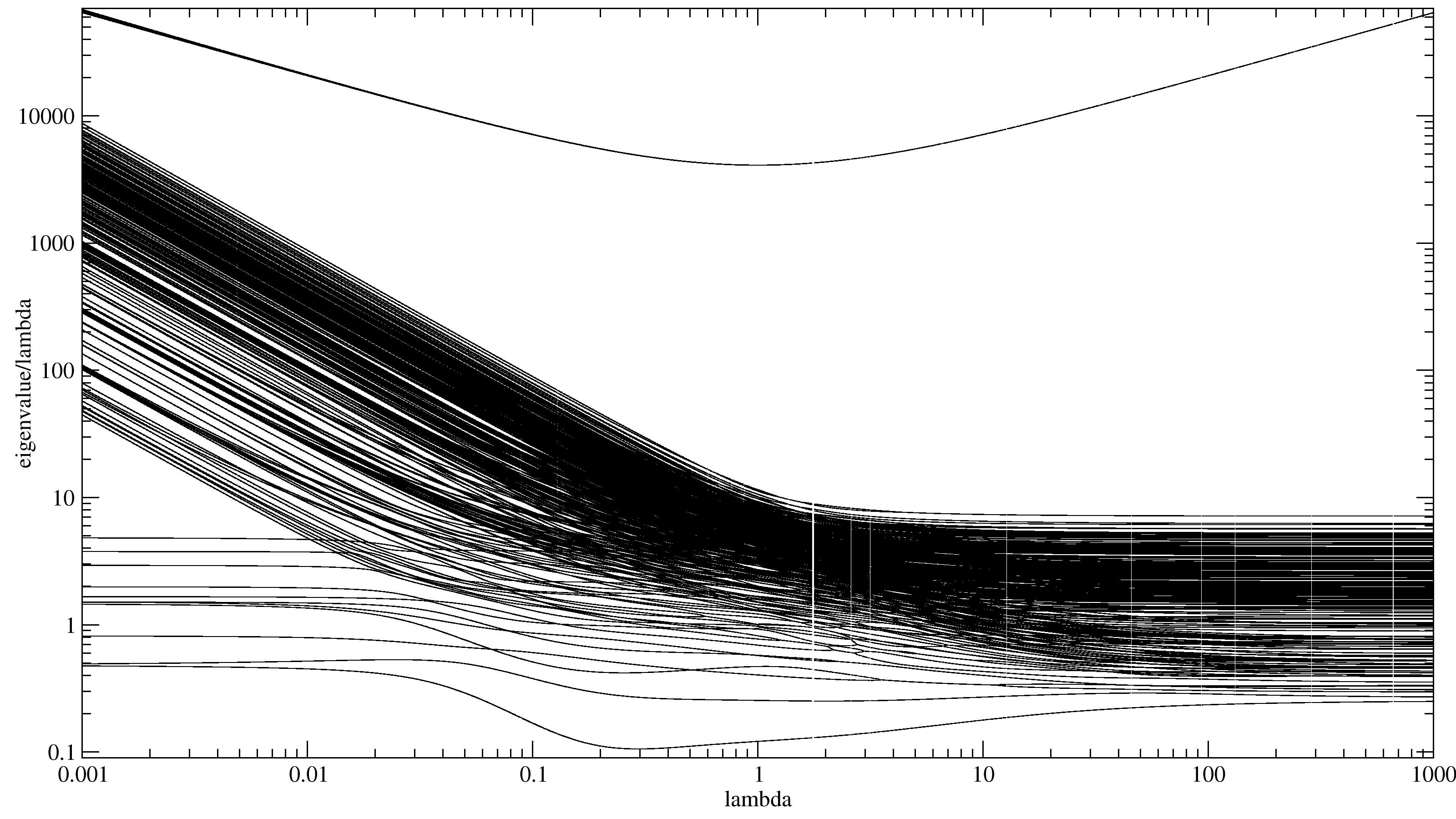
Figure 2: The moduli of the $1024$ eigenvalues of the transition rate matrix with smallest negative real part, as a function of $\lambda$. Moduli are shown divided by $\lambda$ to emphasize the $\mathcal{O}(\lambda)$ and $\mathcal{O}(\lambda^{2})$ trends. There is always a single zero eigenvalue These smallest eigenvalues correspond to the decay rates of the dominant transient states in the system, implying that the time taken for a simulated system to relax to its equilibrium state scales as $\lambda^{-1}$. This helps explain the poor convergence of our Monte Carlo simulations the small-$\lambda$ regime. This data is for system of size $L=8$, $C_{0}=1000$, ($\rho_{0}$, $\rho_{L}$)= (0.6, 0.4)

The near-zero eigenspectrum of the transition rate operator, and its dependence upon $\lambda$ for fixed boundary conditions, is extremely interesting in its own right, as shown in Fig. 2. The structure is rich, with eigenvalues frequently crossing over each other, as well the appearance and disappearance of bands.

Repeat calculations show that large changes in $C_{0}$ cause very small changes in the low-lying eigenspectrum of the transition rate matrix, so in this sense the slow dynamics are insensitive to $C_{0}$. It does affect the group of eigenvalues of larger magnitude, which form a u-shape towards the top of Fig. 2, suggesting that this group is associated with rapid changes in configuration at the boundaries. The extremely large gap between the low-lying and upper sequences of eigenvalues reinforces that notion.

One of the most notable features of the eigenspectrum is the presence of a relatively small number of low-lying eigenvalues which seem to split off from the main sequence as $\lambda$ becomes much smaller than $1$; they have $\mathcal{O}(\lambda)$ scaling, whilst the main sequence has $\mathcal{O}(1)$ scaling. This split coincides with, and may be related to, a suspected transition, which we will discuss in more detail in Section IV.3. System size variations suggest that the number of eigenvalues which belong to this grouping scale as $\mathcal{O}(2^{\sim 0.8L})$, slower than the total number of eigenvalues, $2^{L+4}$, suggesting that they describe long-range phenomena. The split begins as the lowest non-zero eigenvalue takes its lowest values: this may correspond to a change in the character of the flow (i.e. eigenvector of the zero-eigenvector) to include more microstates corresponding to high particle density.

Unfortunately the space complexity of the sparse transition rate matrix scales as $\mathcal{O}(2^{L}L)$, whilst the matrix density scales as $\mathcal{O}(2^{-L}L)$. This makes computations rapidly become unfeasible for large $L$. The overall time complexity for this process is $\mathcal{O}(2^{2L}L)$. In spite of this, we have managed to compute properties such as the steady-state flow rate for systems with sizes as large as $10$ internal lattice sites, which are large enough to produce consistent outputs comparable to our other methods (as shown in Figures 3 and 4), whilst being computationally cheap enough to allow us to perform calculations with many different parameter configurations.

IV Simulations

Given access to large-scale computational hardware, it is relatively straightforward to perform Monte Carlo simulations of the SPM, with a little adjustment to the precise implementation of the model. We chose to calculate primarily by using the KMCLib Leetmaa and Skorodumova (2014) package, which implements the Kinetic Monte Carlo algorithm (essentially the same as the Gillespie algorithm Gillespie (1977); Bortz et al. (1975); Prados et al. (1997)) on lattice systems. The codes used are kept here Hellier (2018).

In the bulk, the transition rates are simply those described in Fig. 1. At the boundaries we used a similar two-layer boundary trick to that described in Sec.III, only this time the particles appear and disappear with rates

$$\sqrt{\lambda\frac{\rho_{0}}{1-\rho_{0}}},$$ (5)

and

$$\sqrt{\lambda\frac{1-\rho_{0}}{\rho_{0}}},$$ (6)

and likewise for $\rho_{L}$, respectively. Whilst it would be nice for these rates to be large in order to force the boundaries to maintain the correct density more accurately, we choose to simply keep them proportional to the geometric mean of $1$ and $\lambda$, otherwise they tend to either happen too rarely or far too frequently, causing the KMC algorithm to be inefficient.

Independent of the KMCLib code, we wrote a simple Metropolis-Hastings algorithm Robert (2015) which randomly selects single particle hops; this is more efficient than using KMC for values of $\lambda$ which are relatively close to $1$ as the algorithm is simple and the acceptance rate is relatively high, so we can generate better statistics using this method in that regime. We calculate the flow from the number of particles entering and leaving the system at the boundaries. Since the model is defined in terms of rates, the flow in “particles per unit time” is a well defined quantity.

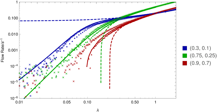
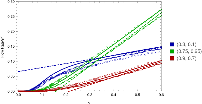
Figure 3: The variation of (normalized) flow rate with $\lambda$ in the SPM with fixed boundary densities, on both logarithmic and linear scales. Crosses indicate results from the KMC simulations, triangles those from the traditional Metropolis-Hastings simulations and the joined circles the current observed the TRM method. The dashed lines are the corresponding MFT predictions for the current, and color indicates the boundary conditions $(\rho_{0},\rho_{L})$ used. Flow rates are normalized to the driving force, so that we can easily compare different system sizes. The standard error in the flow rate is evident from the spread of the points on the graph.

Using KMClib we studied systems of length $64$ (lengths $32$, $128$ and $256$ give similar results as shown in Fig. 6.), running them for $400000$ Gillespie steps for equilibration followed by $10000$ measurement runs of $1000$ steps interspersed with relaxation runs of $16000$ steps. This way we could gather statistics about flow rates and densities in a well-equilibrated system. Specifically, we generate a pool of $10000$ samples of flow rate and density, from which we can calculate estimates of the descriptive statistics of both quantities. These calculations, in which we held the boundary densities constant whilst varying $\lambda$, were repeated using Metropolis-Hastings for a length $100$ system, and we have transition rate matrix currents for a system of length $10$. These are plotted on both logarithmic and linear axes in Fig. 3. respectively.

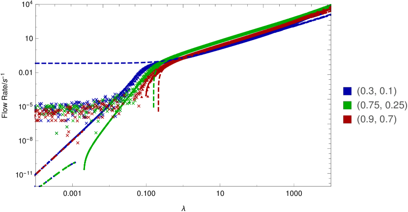
Figure 4: As the logarithmic plot in Fig. 3, but over a much wider range of $\lambda$ values. Notice how the data series from the two Monte-Carlo methods broaden and flatten as $\lambda$ becomes very small; this is because of poor statistics due to the discrete nature of the particles and the extremely low flow rate.

IV.1 Diffusion Coefficient

We compare an MFT prediction (see V) and the KMC numerical results for the diffusion constant in Fig. 9. We see that MFT and simulation agree well for low stickiness, and both show the symmetry about $\rho_{M}=\frac{2}{3}$. For high stickiness, where the MFT prediction gives a negative diffusion constant, we actually see low positive values for the current. It should be noted that the MFT assumes that $\left\langle\rho\right\rangle=\rho_{M}$ throughout, whereas in the simulations $\left\langle\rho\right\rangle$ tends to be much higher.

IV.2 Particle Motion During Flow

It is instructive to get an overview of how the particles move during flow. Fig. 15 show a plot of the flow structure in the slow-flow regime. In very short time averages the “striped” pattern indicates separation into dense and sparse regions, with an overall concentration gradient arising from the relative size of such regions. Particle/vacancy diffusion through the empty/full regions can be seen. As the averages are taken over longer times the blocks themselves appear to diffuse. Averaged over the entire simulation (not shown) the averaging simply gives a smooth density gradient.

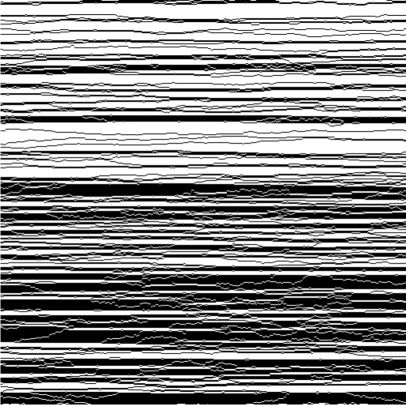
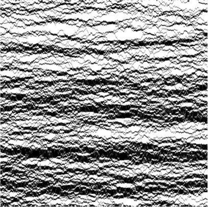
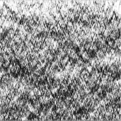
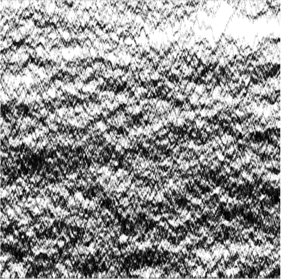
Figure 5: Indicative spacetime flow pattern for sticky free-flow $\left[\lambda=\frac{3}{20},(\rho_{0},\rho_{L})=(\frac{3}{4},\frac{1}{4})\right]$; other combinations shown in the supplementary materials. Time runs along the x-axis, space (1 pixel=1 site) along the y-axis, with grayscale tone (black being empty, white being full) illustrating average site occupation over (clockwise from top left) $\frac{1}{32}$, $1$, $8$ and $32$ Gillespie steps per site respectively.

Interesting structure is visible. The dynamics look like a random walk with some tendency for particles to clump; over longer timescales the diffusive behavior is more evident, with a textured structure suggesting characteristic velocity of particles or vacancies through emergent correlated clumps. Additional plots can be found in the supplementary materials.

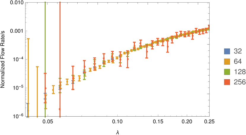
Figure 6: The system size dependence of the normalized flow rate as a function of $\lambda$, computed using the KMC method. These calculations all have boundary conditions $(0.75,0.25)$, and the flow rate has been normalized via multiplication by the system size (displayed on legend). Size $64$ systems are a good compromise in terms of size and accuracy for a given amount of computational time.

IV.3 Transition in flow character

Fig. 4 shows how the current varies with stickiness at fixed driving for a very broad range of $\lambda$. At high $\lambda$ the rate is simply proportional to $\lambda$ for any forcing. This result is far from trivial - it means that the overall flow is determined by the faster rate $(\lambda$), not the slower rate $(1)$. That the MFT averages over the two is unsurprising (Eq. 13), but for the simulation to avoid having a “rate limiting step” requires the system to fill to sufficient density that there are always particles in contact to repel one another, which suggests that the system is performing some kind of self-organization.

When $\lambda=\lambda_{c}\sim 0.2$ the simulations show a transition to a different behavior, with higher or lower $\lambda_{c}$ depending on the boundary conditions and the strength of the driving force. The current and its fluctuation remains finite, but there a distinctive peak in the particle density fluctuation $\left\langle(\rho-\bar{\rho})^{2}\right\rangle$ (Fig. 7). The width of the peak is independent of the system size which suggests a continuous phase transition from the free flowing to the “stuck” regime.

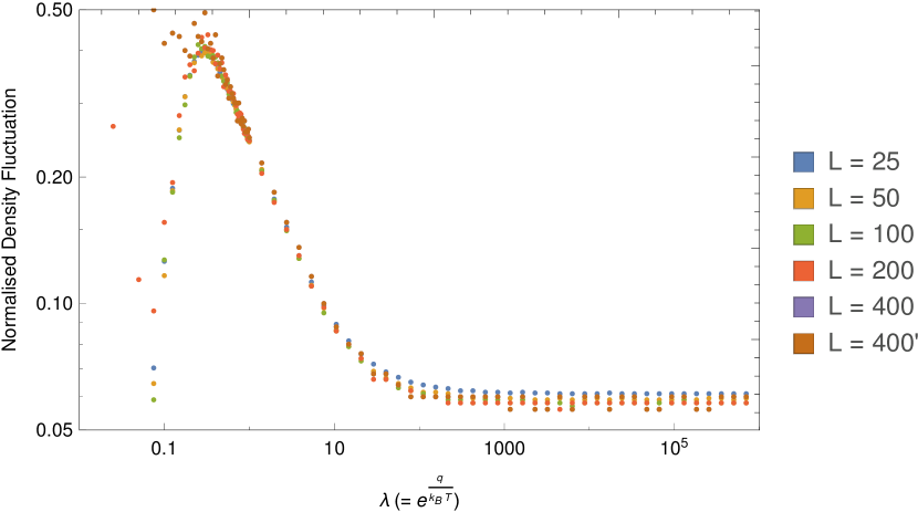
Figure 7: The scaling of the normalized fluctuation in the overall system density with system size, as a function of $\lambda$ and with boundary conditions $(0.6,0.4)$. This was computed using the traditional Metropolis-Hastings method. The normalization was achieved by multiplying by the system size, $L$. The great deal of coherence between these results regardless of size suggests that the fluctuation is of the normal Gaussian type, and not the kind of anomalously-scaling fluctuation associated with equilibrium phase transitions.

Figs. 3 and 4 reveal that in the $(0.3,0.1)$ and $(0.75,0.25)$ boundary configurations the current switches from being $\mathcal{O}(\lambda)$ at high $\lambda$ to being $\mathcal{O}(\lambda^{k})$, $k\sim 4$ for low $\lambda$. In the high-density case, with boundary densities $(0.9,0.7)$, the current actually starts flowing backwards for low $\lambda$ in the transition rate matrix calculation. Therefore, we propose that the peak in the density fluctuation and the odd behavior in the current suggest the existence of a nonequilibrium phase transition in the SPM.

IV.4 Effective diffusion constant

Using boundary conditions

$$(\rho_{0},\rho_{L})=(\rho_{M}+\frac{1}{2}\delta\rho,\rho_{M}-\frac{1}{2}\delta\rho)$$ (7)

we demonstrate the dependence of current on boundary density difference and $\lambda$ (Fig. 8). This shows that the transition to the stuck phase is suppressed by stronger driving forces (large $|\delta\rho|$).

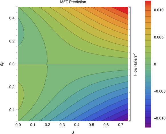
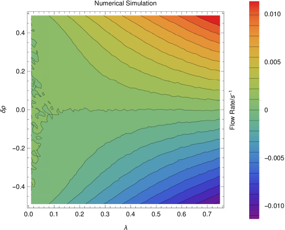
Figure 8: Flow rate mean observed when varying the difference $\delta\rho$ between the boundary concentrations $(\rho_{0},\rho_{L})=(\rho_{M}+\frac{1}{2}\delta\rho,\rho_{M}-\frac{1}{2}\delta\rho)$ and $\lambda$ (The top panel is the MFT prediction for the flow rate, whilst bottom shows the observed mean flow rate). We chose $\rho_{M}=\frac{1}{2}$, as this gives us the biggest range of $\delta\rho$ to investigate. These calculations were performed with the same run parameters (system length etc) as described in Fig. 9. The MFT prediction (top) shows a region of negative flow - this occurs at $\zeta>\frac{4}{5}$ ($\lambda<0.2$) for the weakest driving force, with additional stickiness required when the driving force increases. The simulation exhibits close to zero flow in that region (bottom). Away from this region, the MFT and the simulation are in good agreement.

We use the limit of small $\delta\rho$ to calculate the effective diffusion constant (Fig. 9). This is normalized to 1 in the case of $\lambda=1$, which is just SEP. The $\rho_{M}=0$ limit corresponds to free flow of particles, so the diffusion constant here does to 1. Similarly the $\rho_{M}=1$ limit is flow of vacancies, so $D\rightarrow\lambda$. One might expect a monotonic variation between these limits, but surprisingly the simulations show that there is always an extremal value for $D$ close to $\rho_{M}=2/3$: this is a minimum for $\lambda<1$ and a maximum for $\lambda>1$.

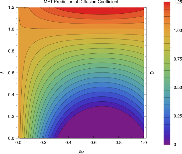
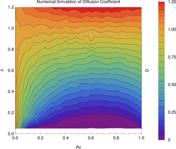
Figure 9: Comparison of effective diffusion coefficient $D$ in the MFT (top) and in direct simulation (bottom) as a function of density and stickiness. The white region is where the MFT gives negative diffusion. The simulations used 124 sites averaged over $\sim 10^{9}$ steps at each of $12\times 24\times 16$ $(\lambda,\rho_{M},\delta\rho)$ combinations. Full details in the supplementary materials.

IV.5 Self-organized density

We calculated the time-averaged total number of particles in the system by updating a histogram of particle numbers as the simulation progresses. In each of our calculations, we make the initial configuration by randomly filling the system with particles and vacancies in such a way that the initial density should be $\frac{1}{2}(\rho_{0}+\rho_{L})$, and then run the system for a sufficient number of equilibration steps to destroy any initial transients.

In SEP, ($\lambda=1$) the density varies linearly across the system from $\rho_{0}$ to $\rho_{L}$, as one expects for a diffusion process. However, for sticky particles, $\lambda<1$, the density rises sharply near to the boundary, then has a linear profile anchored about a value higher than $\rho_{M}$ (Fig. 10). One might view this as particles being sucked into the system to lower their Hamiltonian Energy, but such a notion can be dismissed since the internal density also rises for repelling particles, $\lambda>1$. The asymptotic values for the bulk density at high and low $\lambda$ appear to be 1 and $\frac{2}{3}$ respectively, regardless of the mean boundary density $\rho_{M}$ (see Fig. 11).

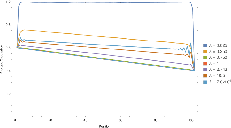
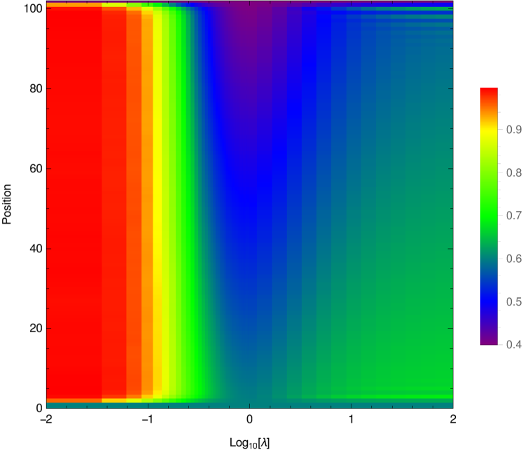
Figure 10: The variation of the time-averaged density profile with respect to $\lambda$. The top panel shows this profile for a selection of values for $\lambda$ in a system of size $100$, with boundary conditions $(0.6,0.4)$; the bottom panel displays this variation in the form of a colored density plot. Again, we have used the traditional Metropolis-Hastings method for these calculations. The oscillatory behavior near the boundary is a robust feature of the profile at high $\lambda$.

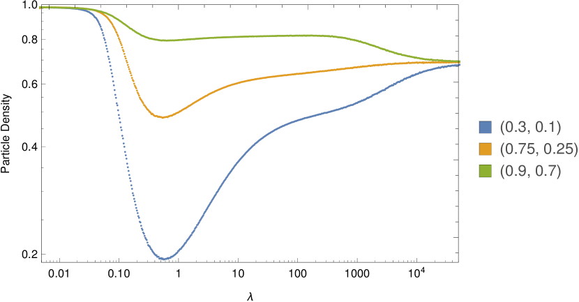
Figure 11: The overall average density of a system of size $64$, computed using KMC, with boundary conditions as specified in the plot. Notice how the density converges to $1$ and $\sim\frac{2}{3}$ for extreme low and high $\lambda$ respectively.

IV.6 Review of the simulations

MC simulation and TRM analysis of the sticky particle model reveals a number of curious and unexpected features which have no equivalent in either SEP or the 1D Ising model.

• A transition in the dependence of the current on $\lambda$ from $\propto\lambda$ to $\propto\lambda^{4}$.

• The mean density of the system has complicated variation with $\lambda$.

• The effective diffusion constant has an extremal value at intermediate boundary density.

To obtain further understanding of these behaviors, we tackle the system analytically, using mean field theory. Although MFT isn’t a particularly sophisticated technique, it does give us a benchmark which we can compare to our other methods.

V Mean Field Theory for Flow

We will be working in the style described in Sec. 2.2 of Blythe and Evans (2007) and Sec. 5.2.2 of Appert-Rolland et al. (2015). Let the spacing between lattice sites be $a$, let $\tau_{0}$ be the free-particle hopping timescale, and the time-averaged (or ensemble-averaged, assuming ergodicity) occupation probability of the $i^{\mathrm{th}}$ lattice site be $\rho_{i}$. We will introduce $\zeta=1-\lambda$ here for convenience.

V.1 Lattice Mean Field Theory

Let the ensemble-averaged occupation probability of the $i^{\mathrm{th}}$ site at time $t$ be $\rho_{i}(t)$. In the mean-field approximation this is assumed to be independent of $\rho_{j}(t)$ for $j\neq i$ at equal times. Therefore, if the $i^{\mathrm{th}}$ site is occupied, then the rate at which it empties is the sum of contributions from the four permutations of the $(i+1)^{\mathrm{th}}$ and $(i-1)^{\mathrm{th}}$ occupancy:

$$\begin{split}&\frac{1}{\tau_{0}}(1-\rho_{i-1})\left[(1-\rho_{i+1})+\lambda\rho_{i+1}\right]\\ +&\frac{1}{\tau_{0}}(1-\rho_{i+1})\left[(1-\rho_{i-1})+\lambda\rho_{i-1}\right].\end{split}$$ (8)

Similarly, if the $(i)^{\mathrm{th}}$ site is unoccupied, it fills with rate which depends on the occupation probability of the neighbours, and whether they are stuck to the $(i+2)^{\mathrm{th}}$ and $(i-2)^{\mathrm{th}}$ sites respectively. Therefore, an unoccupied $i^{\mathrm{th}}$ site fills with rate

$$\frac{1}{\tau_{0}}\left\{\rho_{i+1}\left[\lambda\rho_{i+2}+(1-\rho_{i+2})\right]+\rho_{i-1}\left[\lambda\rho_{i-2}+(1-\rho_{i-2})\right]\right\}.$$ (9)

If we now multiply the filling/emptying rates of site $i$ by the probability of being empty/full respectively, we obtain the final equation for the site occupation

$$\begin{split}\tau_{0}\frac{\partial\rho_{i}}{\partial t}&=\left(1-\rho_{i}\right)\left[\left(1-\zeta\rho_{i-2}\right)\rho_{i-1}+\left(1-\zeta\rho_{i+2}\right)\rho_{i+1}\right]\\ &-\rho_{i}\left[2\zeta\rho_{i-1}\rho_{i+1}-(3-\zeta)\left(\rho_{i-1}+\rho_{i+1}\right)+2\right].\end{split}$$ (10)

V.2 Diffusion Equation: MFT Continuum Limit

To obtain the continuum limit of the MFT we substitute $\rho_{i}(t)\rightarrow\rho(x,t)$, $\rho_{i+m}(t)\rightarrow\rho(x+am,t)$ into Eq. 10. Then, using a Taylor expansion around $x$ for small $a$, neglecting terms of $\mathcal{O}(a^{4})$, and collecting terms we find that

$$\begin{split}\tau_{0}\frac{\partial\rho}{\partial t}=&a^{2}\left[1-\zeta\rho(4-3\rho)\right]\frac{\partial^{2}\rho}{\partial x^{2}}\\ +&2a^{2}\zeta(3\rho-2)\left(\frac{\partial\rho}{\partial x}\right)^{2}+\mathcal{O}(a^{4}),\end{split}$$ (11)

which can be factorized into the more familiar form of a continuity equation

$$\frac{\partial\rho}{\partial t}=\frac{a^{2}}{\tau_{0}}\frac{\partial}{\partial x}\left\{\left[1-\zeta\rho\left(4-3\rho\right)\right]\frac{\partial\rho}{\partial x}\right\},$$ (12)

having dropped the higher-order terms. From this we can identify the flow $J(x)$ as the term in the curly brackets, and define a mean field diffusion constant (see Fig.9):

$$D(\zeta,\rho)=\frac{a^{2}}{\tau_{0}}\left[1-\zeta\rho\left(4-3\rho\right)\right]$$ (13)

We note that the MFT diffusion constant can become negative. The density at which this occurs is given by finding the roots $\rho_{c}$ of the RHS of Eq. 13:

$$\rho_{c}=\frac{2}{3}\pm\frac{1}{3}\sqrt{(}4-3/\zeta).$$ (14)

The possible values for $\rho_{c}$ are only real (and therefore physically possible) for $\zeta<0.75$. So in the limit of very sticky particles ($\lambda<0.25$) the MFT predicts a transition between forward and backwards diffusion at some densities.

V.3 Limiting Cases

In order to understand the implications of the MFT, let us consider some limits. As $\zeta\rightarrow 0$ (i.e. as the model becomes a simple exclusion model), $D\rightarrow\frac{a^{2}}{\tau_{0}}$. Likewise, in the dilute limit $\rho\rightarrow 0$, $D\rightarrow\frac{a^{2}}{\tau_{0}}$, reflecting the fact that it becomes a dilute lattice gas and therefore the interactions between particles become irrelevant as they never meet. Conversely, in the full limit $\rho\rightarrow 1$, $D\rightarrow\frac{\lambda a^{2}}{\tau_{0}}$; this is because we now have a dilute gas of vacancies, which hop with rate $\frac{\lambda}{\tau_{0}}$.

One may observe that the MFT has a symmetry under $\rho\mapsto\frac{4}{3}-\rho$; thus, the dynamics should be symmetric under a density profile reflection around $\rho=\frac{2}{3}$. This is where $D$ always attains its extremal value, $\frac{a^{2}}{\tau_{0}}\left[1-\frac{4}{3}\zeta\right]$, hence for $\zeta>3/4$ the diffusion coefficient becomes negative in regions with $\frac{2}{3}-\frac{\sqrt{\zeta\left(4\zeta-3\right)}}{3\zeta}<\rho<\frac{2}{3}+\frac{\sqrt{\zeta\left(4\zeta-3\right)}}{3\zeta}$.

Finally, it is possible to show that solutions to the continuum MFT containing domains with a negative diffusion coefficient are linearly unstable; thus, if we try to have a flow containing $\rho$ for which $D(\rho)<0$, the density of the medium should gravitate towards one of the two densities for which $D(\rho)\sim 0$. Instead of observing “backwards diffusion” we would see an extremely slow flow or no flow at all.

V.4 Steady State Flow

It is possible to solve the continuum MFT in a steady state on a finite domain, say $x\in(0,L)$. Steady state implies that there is no build-up of particles $\frac{\partial\rho}{\partial t}=0$, so the flow is constant through the system.

Using the constant-flow requirement for continuity $J(x)=J_{0}=\mathrm{const.}$, and by integrating both sides of Eq. 12 with respect to $x$ we find that

$$\int_{x_{0}}^{x}J(x^{\prime})dx^{\prime} = -\frac{a^{2}}{\tau_{0}}\int\!\!\mathrm{d}\rho\left[1-\zeta\rho\left(4-3\rho\right)\right]$$ (15)

$$(x-x_{0})J_{0} = -\frac{a^{2}}{\tau_{0}}\left[\rho+\zeta(\rho-2)\rho^{2}\right].$$ (16)

The density profile across the system is given by solving for $\rho(x)$. Since Eq.16 is cubic, the solution for density $\rho(x)$ is non-unique for cases of high $\zeta$. Thus in the limit of high stickiness, the MFT is unable to make a unique prediction for the density. Furthermore, except in the SEP case $\zeta=0$, the density will not vary linearly across the system.

V.5 Dirichlet Boundary Conditions

The constants $x_{0}$ and $J_{0}$ relate to the boundary conditions for the flow, but they need not correspond to a physically-realizable situation. For driven systems it is more convenient to consider fixing the density at each end.

If we impose such Dirichlet boundary conditions on this system, say $\rho(0)=\rho_{0}$ and $\rho(L)=\rho_{L}$, we find that

$$J_{0}=\frac{a^{2}}{L\tau_{0}}\left[\rho_{0}-\rho_{L}+\zeta\left(\rho_{0}\left[\rho_{0}^{2}-2\right]-\rho_{L}\left[\rho_{L}^{2}-2\right]\right)\right].$$ (17)

This equation can be used for direct comparison with the simulations (Fig. 8 and Fig. 9). In general, the agreement is good, except for the region where the MFT predicts negative flow.

V.6 Interpretation of MFT

The mean field theory enables us to predict flow behavior of the SPM. It recovers well-known limiting cases such as SEP ($\lambda=0$), however at high stickiness ($\lambda<0.25$) it predicts its own demise, with unphysical negative diffusion constants and by having multiple solutions for the density at some positions in the system, meaning that the MFT does not give a unique density profile. This breakdown of the MFT corresponds to the transition to slow flow observed in the simulation.

In some conditions MFT predicts densities greater than 1. One might guess that when the MFT offers two possible values for the density, it will correspond to a phase separation in the actual system. Furthermore, the MFT prediction of a maximum diffusion constant at a density of $\rho=2/3$ suggests that this value of $\rho$ might be favored for strongly driven flows.

A curious feature of the MFT diffusion (Fig. 9) is that for fixed stickiness there are two possible densities giving the same diffusion constant. Thus it is possible to have a steady state flow with phase separation into regions of high and low density. This echoes the situation seen in short time-averages of the simulation (Fig.15) where blocks of high and low density are evident, as well as the oscillatory behavior near the boundaries at high $\lambda$ (Fig. 10).

Regarding the phase transition, we should note that we only have an MFT prediction for the flow rate for $\lambda>\frac{1}{4}$, since $\rho(x)$ stops being unique when $\lambda$ drops below $\frac{1}{4}$. For higher $\lambda$, the MFT is broadly in good agreement with the simulations, and this continues as $\lambda$ stretches into the thousands, where the mean flow varies as $\mathcal{O}(\lambda^{1})$.

The MFT prediction for the mean flow continues to be a good fit until $\lambda$ becomes sufficiently small, when the simulations show no evidence of negative diffusion; rather the flow becomes critically slow for very sticky particles. The higher moments of the simulated flow (e.g. variance) do not show peaks, indicating that hard transitions are not occurring. Finally, the simulated density is very close to the average of the boundary densities until $\lambda$ drops below 1/4, at which point the system fills.

VI Discussion

We have analysed the model using three methods: Direct simulation, Transition rate matrices and mean field theory. Each has advantages and drawbacks, but all show a nonequilibrium transition between a free-flowing and a blocked phase. In direct simulation this appears as a peak in the energy and density fluctuations and a change from $~{}\lambda$ to $~{}\lambda^{4}$ dependence in the flow rate. In MFT it appears as a negative diffusion constant. In the TRM it corresponds to a minimum in the minimum eigenvalue, and a crossover in the character of the associated eigenvector, as clearly illustrated in Figure.15

The MFT suggests a symmetry between vacancy-type and particle-type flow at density of $\frac{2}{3}$, which is observed in the MC simulations and TRM calculations. The density self-organizes to this value in the limit of strongly repelling particles.

The continuum limit solution to the MFT is a good predictor of the bulk flow behavior of the SPM for high $\lambda$. The negative diffusion constant found in MFT at high stickiness indicates that the assumption of homogeneous density breaks down: thus the MFT predicts its own demise at a point which agrees well with the numerics.

Above a certain level of stickiness, the model exhibits a nonequilibrium phase transition to a slow-flowing phase. The required stickiness for the transition is dependent on the strength of the driving force - large differences between the boundary densities push the transition towards higher stickiness. Mean field analysis, together with visualization of the flowing system, suggest that the transition occurs when the density becomes inhomogeneous.

The flow exhibits a foamy pattern with time-and-space correlations of intermediate size. The open boundary condition means the system self-organizes its density. At zero interaction ($\lambda=1$) this must be the mean of the boundary conditions, and it is unsurprising that high stickiness means the system fills. Strong repulsion between the particles leads to a density of $\frac{2}{3}$, which appears to maximize the flow rate at high $\lambda$; there is no known physical principle which requires this.

VII Conclusions

The sticky particle model is the combination of the Ising model with the symmetric exclusion process. It represents the simplest possible flow model for interacting particles in a homogeneous medium, and as such is a model for many physical systems where particles are driven by a pressure or concentration difference across the boundaries.

We have shown that it exhibits complicated and discontinuous behaviour absent in either 1D Ising or SEP model, specifically, a transformation from fast to slow flow with stickiness.

A number of questions remain open. Is there a physical principle which determines the density (Fig. 10)? Why does the strongly repelling system produce a density with maximum flow (Fig. 11)? Can one derive the $~{}\lambda^{4}$ dependence of the slow-flow (Fig. 4)? These clear, emergent results from our detailed work strongly suggest that there is a higher level description of complex flow which could predict them, but to our knowledge no such unifying theory of nonequilibium thermodynamics exists.

Appendix A Linear Stability of MFT Solution.

Let $\rho_{0}(x)$ be a solution to the steady-state continuum MFT, and let us apply a small perturbation $\delta\rho(x,t)$. Let us also assume that $\rho_{0}$ is also slowly-varying in $x$, in the sense that $\delta\rho=o(\rho_{0})$ and $\frac{\partial\rho_{0}}{\partial x}=o(\delta\rho)$, which should be approximately true for a large domain. Then substituting $\rho=\rho_{0}+\delta\rho$ into the continuum-limit MFT and only the highest-order terms, we find that

$$\frac{\partial\delta\rho}{\partial t}=\frac{a^{2}}{\tau_{0}}\rho_{0}(4-3\zeta\rho_{0})\frac{\partial^{2}\delta\rho}{\partial x^{2}}+o(\delta\rho).$$ (18)

Performing a Fourier transform (or rather, a suitable local equivalent) with respect to $x$ to yield $\hat{\delta\rho}(k,t)=\mathcal{F}\left[\delta\rho(x,t)\right]$, this becomes

$$\frac{\partial\hat{\delta\rho}}{\partial t}=-k^{2}\frac{a^{2}}{\tau_{0}}\rho_{0}(4-3\zeta\rho_{0})\hat{\delta\rho}.$$ (19)

This means that so long as $\zeta<\frac{3}{4}$, the RHS is always negative, and therefore small perturbations decay exponentially and all is well. However, if $\zeta>\frac{3}{4}$, there may be regions of the solution where $\rho_{0}(4-3\zeta\rho_{0})$ becomes negative, causing small perturbations to grow exponentially with an emphasis on high-wavenumber (short-lengthscale) modes, which indicates linear instability.

Appendix B Additional Flow Data.

Fig. 12, 13 and 14 display additional data and information from computations discussed in the main body of the paper. These were performed with KMC using the same run parameters as those used to create Fig. 3.

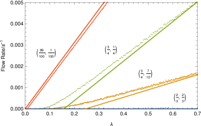
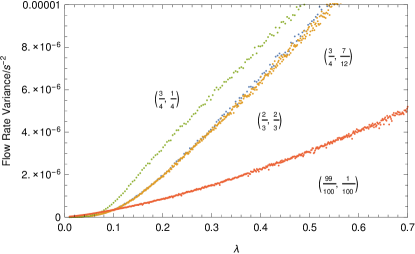
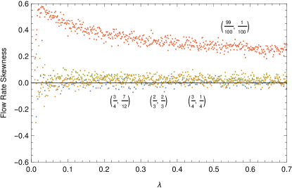
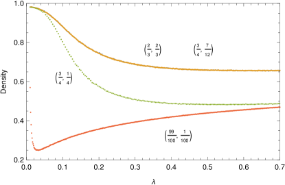
Figure 12: Additional flow rate moments and overall system densities for the sweeps through $\lambda$ with fixed boundaries.

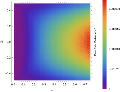
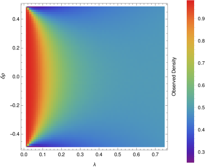
Figure 13: Flow rate variance and average overall densities observed when varying the difference $\delta\rho$ between the boundary concentrations $(\rho_{B},\rho_{T})=(\rho_{M}+\frac{1}{2}\delta\rho,\rho_{M}-\frac{1}{2}\delta\rho)$ and $\lambda$. $\rho_{M}=\frac{1}{2}$, as in the paper.

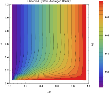
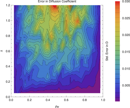
Figure 14: These images are in addition to our computation of the effective diffusion coefficient $D$. The left shows the overall system density as a function of $\rho_{M}$ and $\lambda$, whilst the right shows the standard error in our estimate of $D$. In this setup we ran the KMC simulation for $1.6\times 10^{8}$ equilibration steps, followed by $10$ sets of alternating measurement and relaxation runs, of lengths $8\times 10^{7}$ and $1.6\times 10^{7}$ steps respectively. These results are consistent with calculations performed on smaller systems, so finite-size effects should be suppressed.

Appendix C More flow plots.

For the interested reader we have included for spacetime flow diagrams, show in Fig. 15. When $\lambda=0.05$, the medium consists of solid blocks surrounded by empty spaces containing a dilute gas of particles; at $\lambda=0.35$ it is not so different from normal diffusion. The most interesting images are those for the intermediate $\lambda$; here we see a “lumpy” or “foamy” structure, in which small blocks of particles are being constantly created and destroyed whilst a rather minimal flow occurs across the system. The simulations did not show any hard phase transition as we vary $\lambda$; rather, it seems that this “foamy” behavior is part of a continuous range between the extremes, containing medium-range correlations between particles. Unfortunately, computing equal-time correlation functions to the accuracy required to draw conclusions about these correlations has proven to be extremely difficult, so we cannot find a quantitative description of the foam beyond the flow rate and density data we have discussed in this paper. In all images in Fig. 15, long straight segments of white of black can be seen. The represent coherent motion at a characteristic velocity given by their gradient. There is nothing in the MFT to suggest what this velocity should be, and it is much smaller than the simulated system’s length divided by the elapsed time, $\frac{L}{T}$, thus it must be an emergent property arising from correlated motion of self-assembled regions of high- or low-density material. However, it has again proved difficult to analyze this numerically.

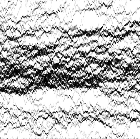
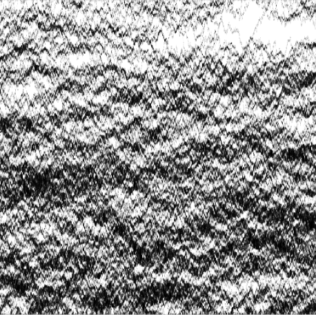
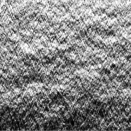
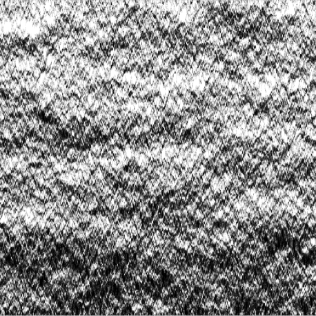
Figure 15: The spacetime flow patterns, for $\lambda$-values of $0.05$, $0.15$, $0.25$ and $0.35$ going clockwise from top left. In each plot time runs along the $x$-axis, space along the $y$-axis, with the bottom boundary being held with a concentration of $\frac{1}{4}$ and the top at $\frac{3}{4}$. White represents full occupation, black empty, and gray shades partial occupation. The degree of occupation was calculated by taking the KMCLib record of a particular site’s occupation (i.e. the Gillespie times at which the site changed occupation), assigning $0$ and $1$ to particles and vacancies respectively, linearly interpolating this and then integrating over times longer than a single Gillespie step but much shorter than the total time in question. In each case the total time elapsed is that taken by $2^{6}$ Gillespie steps, and each short-time-average has been done over the total time divided by $512$, the number of lattice sites; this means that on average a site would change state 8 times per pixel, although of course the real distribution is not nearly this even. Time has been rescaled this way in order to allow fair comparison of different $\lambda$-values.

Appendix D Non-Uniqueness of the MFT Density Profile.

Recall that, according to the MFT,

$$\int\!\!\mathrm{d}x\ J(x)=(x-x_{0})J_{0}=-\frac{a^{2}}{\tau_{0}}\rho\left[1+\zeta\rho\left(\rho-2\right)\right],$$ (20)

which we would like to solve for $\rho(x)$. We can do this uniquely so long as the right hand side is monotonic for $\rho\in(0,1)$. Monotonicity requires that the sign of the derivative of the RHS wrt $\rho$ does not change in that region. This derivative is of course

$$\frac{\mathrm{d}\mathrm{RHS}}{\mathrm{d}\rho} =-\frac{a^{2}}{\tau_{0}}\rho\left[1+\zeta\rho\left(\rho-2\right)\right]$$ (21)

$$=-\frac{a^{2}}{\tau_{0}}\left[3\zeta(\rho-\frac{2}{3})^{2}+(1-\frac{4}{3}\zeta)\right].$$ (22)

The term in square brackets is always $1$ at $\rho=0$ and $\lambda$ at $\rho=1$, which are both positive. If $\zeta<0$, the term is an n-shaped parabola with both boundaries positive; therefore it is always positive, and there is no sign change. For $\zeta>0$ (the case of interest for us), we can see from completing the square that the term is always positive unless $\zeta>\frac{3}{4}$, in which case there is a sign change and therefore a loss of monotonicity. Thus for $\zeta>\frac{3}{4}$ (and correspondingly $\lambda<\frac{1}{4}$) the MFT does not have a unique steady state solution given a set of Dirichlet boundary conditions, and so we cannot expect the MFT to predict the density profile in that regime.

Appendix E Particle Density in Bounded Domain at Extreme $\lambda$-Values.

We scanned across a wide range of $\lambda$ with three sets of boundary conditions: $(\frac{3}{10},\frac{1}{10})$, $(\frac{3}{4},\frac{1}{4})$ and $(\frac{9}{10},\frac{7}{10})$. The resulting mean flow rate is shown in Fig. 16, and the corresponding density results were already displayed. We once again see the transitions between power law behaviors, as discussed in the main body of the paper. Note that the MFT is never a particularly good fit for the $(\frac{3}{4},\frac{1}{4})$ configuration; this may be because the difference between the boundaries is greater than in the other cases. The other MFTs are good fits in the high-$\lambda$ regime until we start reaching $\lambda~{}\sim~{}1000$, at which point they seem to start converging to the same flow regardless of boundary conditions. In each case for low-$\lambda$ we have a power-law regime, each with with an exponent around $4$, and then at extreme low-$\lambda$ we lose a consistent signal because of noise, which we attribute to lack of system convergence due to critically slow flow.

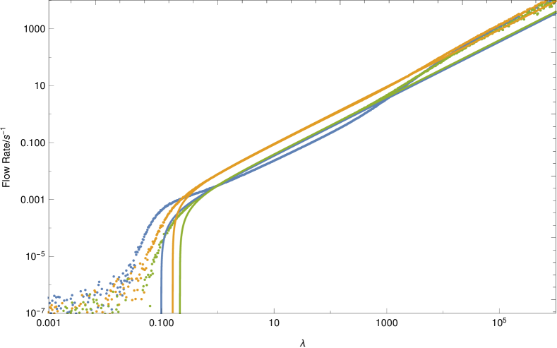
Figure 16: Flow rate as a function of $\lambda$ for systems with boundary conditions $(\frac{3}{10},\frac{1}{10})$, $(\frac{3}{4},\frac{1}{4})$ and $(\frac{9}{10},\frac{7}{10})$, colored in blue, gold and green respectively.

So far as the density is concerned, at $\lambda=1$ in each case it is about what we would expect (the average of the two boundary densities). It is minimized around $\lambda=0.6$, and then as $\lambda$ is reduced each density appears to converge to $1$ regardless of boundary conditions (before we encounter the same convergence issue at extreme low-$\lambda$). As we go to high-$\lambda$, on the other hand, we see a similar convergence, but this time towards $\rho\sim 0.7$. This is interesting, as a density of $\rho=\frac{2}{3}$ is predicted by the MFT to be where maximal flow should occur for $\lambda>1$; thus it would appear that the system self-organizes to facilitate maximal flow, which is something which is hypothesized to occur in other nonequilibrium statmech systems. This also helps to explain the large deviations from the MFT flow predictions we encounter at high-$\lambda$, as the system in practice has a different density to the one assumed by the MFT.

References

- Belitsky and Schütz (2011) V Belitsky and G M Schütz, “Cellular automaton model for molecular traffic jams,” Journal of Statistical Mechanics: Theory and Experiment 2011, P07007 (2011).
- Mobilia et al. (2007) Mauro Mobilia, Ivan T. Georgiev, and Uwe C. Täuber, “Phase transitions and spatio-temporal fluctuations in stochastic lattice lotka–volterra models,” Journal of Statistical Physics 128, 447–483 (2007).
- Tegner et al. (2015) B. E. Tegner, L. Zhu, C. Siemers, K. Saksl, and G. J. Ackland, “High temperature oxidation resistance in titanium-niobium alloys,” Journal of alloys and compounds 643, 100–105 (2015).
- Zhu et al. (2012) Linggang Zhu, Qing-Miao Hu, Rui Yang, and Graeme J. Ackland, “Atomic-scale modeling of the dynamics of titanium oxidation,” Journal of Physical Chemistry C 116, 24201–24205 (2012).
- Deal and Grove (1965) B. E. Deal and A. S. Grove, “General relationship for the thermal oxidation of silicon,” Journal of Applied Physics 36, 3770–3778 (1965), https://doi.org/10.1063/1.1713945 .
- Cabrera and Mott (1949) N Cabrera and N F Mott, “Theory of the oxidation of metals,” Reports on Progress in Physics 12, 163 (1949).
- Buzzaccaro et al. (2007) Stefano Buzzaccaro, Roberto Rusconi, and Roberto Piazza, ““sticky” hard spheres: Equation of state, phase diagram, and metastable gels,” Phys. Rev. Lett. 99, 098301 (2007).
- Ladd et al. (1988) Anthony J. C. Ladd, Michael E. Colvin, and Daan Frenkel, “Application of lattice-gas cellular automata to the brownian motion of solids in suspension,” Phys. Rev. Lett. 60, 975–978 (1988).
- Liggett (1985) Thomas M Liggett, Interacting particle systems (Springer-Verlag, Berlin, 1985).
- Ben-Naim et al. (1999) E. Ben-Naim, S. Y. Chen, G. D. Doolen, and S. Redner, “Shocklike dynamics of inelastic gases,” Phys. Rev. Lett. 83, 4069–4072 (1999).
- Shandarin and Zeldovich (1989) S. F. Shandarin and Ya. B. Zeldovich, “The large-scale structure of the universe: Turbulence, intermittency, structures in a self-gravitating medium,” Rev. Mod. Phys. 61, 185–220 (1989).
- Frachebourg (1999) L. Frachebourg, “Exact solution of the one-dimensional ballistic aggregation,” Phys. Rev. Lett. 82, 1502–1505 (1999).
- Frachebourg et al. (2000) L. Frachebourg, P. A. Martin, and J. Piasecki, “Ballistic aggregation: a solvable model of irreversible many particles dynamics,” Physica A Statistical Mechanics and its Applications 279, 69–99 (2000), cond-mat/9911346 .
- Obukhovsky et al. (2017) Vyacheslav V. Obukhovsky, Andrii M. Kutsyk, Viktoria V. Nikonova, and Oleksii O. Ilchenko, “Nonlinear diffusion in multicomponent liquid solutions,” Phys. Rev. E 95, 022133 (2017).
- Gorokhova and Melnik (2010) N. V. Gorokhova and O. E. Melnik, “Modeling of the dynamics of diffusion crystal growth from a cooling magmatic melt,” Fluid Dynamics 45, 679–690 (2010).
- Kardar et al. (1986) Mehran Kardar, Giorgio Parisi, and Yi-Cheng Zhang, “Dynamic scaling of growing interfaces,” Phys. Rev. Lett. 56, 889–892 (1986).
- Krug and Spohn (1988) J. Krug and H. Spohn, “Universality classes for deterministic surface growth,” Phys. Rev. A 38, 4271–4283 (1988).
- Sasamoto and Spohn (2010) Tomohiro Sasamoto and Herbert Spohn, “One-dimensional kardar-parisi-zhang equation: An exact solution and its universality,” Phys. Rev. Lett. 104, 230602 (2010).
- Sugden and Evans (2007) K E P Sugden and M R Evans, “A dynamically extending exclusion process,” Journal of Statistical Mechanics: Theory and Experiment 2007, P11013 (2007).
- Kollmann (2003) Markus Kollmann, “Single-file diffusion of atomic and colloidal systems: Asymptotic laws,” Phys. Rev. Lett. 90, 180602 (2003).
- Lin et al. (2005) Binhua Lin, Mati Meron, Bianxiao Cui, Stuart A. Rice, and Haim Diamant, “From random walk to single-file diffusion,” Phys. Rev. Lett. 94, 216001 (2005).
- Hegde et al. (2014) Chaitra Hegde, Sanjib Sabhapandit, and Abhishek Dhar, “Universal large deviations for the tagged particle in single-file motion,” Phys. Rev. Lett. 113, 120601 (2014).
- Krapivsky et al. (2014) P. L. Krapivsky, Kirone Mallick, and Tridib Sadhu, “Large deviations in single-file diffusion,” Phys. Rev. Lett. 113, 078101 (2014).
- Imamura et al. (2017) Takashi Imamura, Kirone Mallick, and Tomohiro Sasamoto, “Large deviations of a tracer in the symmetric exclusion process,” Phys. Rev. Lett. 118, 160601 (2017).
- Katz et al. (1984) Sheldon Katz, Joel L. Lebowitz, and Herbert Spohn, “Nonequilibrium steady states of stochastic lattice gas models of fast ionic conductors,” Journal of Statistical Physics 34, 497–537 (1984).
- Zia (2010) R. K. P. Zia, “Twenty five years after kls: A celebration of non-equilibrium statistical mechanics,” Journal of Statistical Physics 138, 20–28 (2010).
- Kafri et al. (2003) Y. Kafri, E. Levine, D. Mukamel, G. M. Schütz, and R. D. Willmann, “Phase-separation transition in one-dimensional driven models,” Phys. Rev. E 68, 035101 (2003).
- Kawasaki (1966) Kyozi Kawasaki, “Diffusion constants near the critical point for time-dependent ising models. i,” Phys. Rev. 145, 224–230 (1966).
- Spohn (1983) H Spohn, “Long range correlations for stochastic lattice gases in a non-equilibrium steady state,” Journal of Physics A: Mathematical and General 16, 4275 (1983).
- Leetmaa and Skorodumova (2014) M. Leetmaa and N. V. Skorodumova, “KMCLib: A general framework for lattice kinetic Monte Carlo (KMC) simulations,” Computer Physics Communications 185, 2340–2349 (2014), arXiv:1405.1221 [physics.comp-ph] .
- Gillespie (1977) Daniel T. Gillespie, “Exact stochastic simulation of coupled chemical reactions,” The Journal of Physical Chemistry 81, 2340–2361 (1977), http://dx.doi.org/10.1021/j100540a008 .
- Bortz et al. (1975) A.B. Bortz, M.H. Kalos, and J.L. Lebowitz, “A new algorithm for monte carlo simulation of ising spin systems,” Journal of Computational Physics 17, 10 – 18 (1975).
- Prados et al. (1997) A. Prados, J. J. Brey, and B. Sánchez-Rey, “A dynamical monte carlo algorithm for master equations with time-dependent transition rates,” Journal of Statistical Physics 89, 709–734 (1997).
- Hellier (2018) Joshua Hellier, “joshuahellier/phdstuff: Codes for sticky particles in 1d and 2d,” (2018), 10.5281/zenodo.1162818.
- Robert (2015) Christian P. Robert, “The metropolis-hastings algorithm,” in Wiley StatsRef: Statistics Reference Online (American Cancer Society, 2015) pp. 1–15.
- Blythe and Evans (2007) R A Blythe and M R Evans, “Nonequilibrium steady states of matrix-product form: a solver’s guide,” Journal of Physics A: Mathematical and Theoretical 40, R333 (2007).
- Appert-Rolland et al. (2015) Cécile Appert-Rolland, Maximilian Ebbinghaus, and Ludger Santen, “Intracellular transport driven by cytoskeletal motors: General mechanisms and defects,” (2015).