A Chandra Survey of Milky Way Globular Clusters I: Emissivity and Abundance of Weak X-ray Sources

Abstract

Based on archival Chandra data, we have carried out an X-ray survey of 69, or nearly half the known population of, Milky Way globular clusters (GCs), focusing on weak X-ray sources, mainly cataclysmic variables (CVs) and coronally active binaries (ABs). Using the cumulative X-ray luminosity per unit stellar mass (i.e., X-ray emissivity) as a proxy of the source abundance, we demonstrate a paucity (lower by $41\%\pm 27\%$ on average) of weak X-ray sources in most GCs relative to the field, which is represented by the Solar neighborhood and Local Group dwarf elliptical galaxies. We also revisit the mutual correlations among the cumulative X-ray luminosity ($L_{X}$), cluster mass ($M$) and stellar encounter rate ($\Gamma$), finding $L_{X}\propto M^{0.74\pm 0.13}$, $L_{X}\propto\Gamma^{0.67\pm 0.07}$ and $\Gamma\propto M^{1.28\pm 0.17}$. The three quantities can further be expressed as $L_{X}\propto M^{0.64\pm 0.12}\ \Gamma^{0.19\pm 0.07}$, which indicates that the dynamical formation of CVs and ABs through stellar encounters in GCs is less dominant than previously suggested, and that the primordial formation channel has a substantial contribution. Taking these aspects together, we suggest that a large fraction of primordial, soft binaries have been disrupted in binary-single or binary-binary stellar interactions before they can otherwise evolve into X-ray-emitting close binaries, whereas the same interactions also have led to the formation of new close binaries. No significant correlations between $L_{X}/L_{K}$ and cluster properties, including dynamical age, metallicity and structural parameters, are found.

1. Introduction

Globular clusters (GCs) are aged and self-gravitationally bound systems that evolve with a high stellar density. Since the launch of the first X-ray satellite, Uhuru, it has been recognized that the abundance (i.e., number per unit stellar mass) of luminous X-ray binaries (with luminosity $L_{\rm X}\gtrsim 10^{36}{\rm\ erg\,s^{-1}}$) in GCs is $\sim$100 times higher than in the Galactic field (Clark, 1975; Katz, 1975). This over-abundance was attributed to the efficient formation of low-mass X-ray binaries (LMXBs) by stellar dynamical interactions in the dense core of GCs, where an isolated neutron star can be captured by a main sequence star through tidal force (Fabian et al., 1975), by a giant through collision (Sutantyo, 1975), or by a primordial binary through exchange with one of the constituent stars (Hills, 1976). The fundamental parameter quantifying these dynamical interactions is the so-called stellar encounter rate, $\Gamma$, which is related to the stellar density ($\rho$) and velocity dispersion ($\sigma$), as $\Gamma\propto\int{\rho}^{2}/\sigma$, an integral over the cluster volume.

With its superb angular resolution and sensitivity, the Chandra X-ray Observatory has resolved a large number of low-luminosity ($L_{X}\lesssim 10^{34}{\rm\ erg\ s^{-1}}$) source in GCs. When deep HST optical/ultraviolet images are available, the majority of these weak X-ray sources are found to be cataclysmic variables (CVs) and coronally active binaries (ABs), the rest being quiescent LMXBs (qLMXBs) and millisecond pulsars (MSPs) (e.g., Grindlay et al., 2001; Pooley et al., 2002a; Edmonds et al., 2003; Heinke et al., 2003, 2005; Haggard et al., 2009; Maxwell et al., 2012). These stellar systems either are experiencing the drastical binary evolution stage (i.e., qLMXBs, CVs, ABs) or are the immediate remnants of close binaries (i.e., MSPs), hence their formation could also have been affected by dynamical processes in GCs. Indeed, previous work revealed a correlation between the number of detected X-ray sources, in particular CVs, and the stellar encounter rate (Pooley et al., 2003; Heinke, 2006; Maxwell et al., 2012), which was interpreted as a dominant fraction of these sources originating from dynamical processes (Pooley & Hut, 2006).

However, it remains an open question of which dynamical process(es) is primarily responsible for the above correlation. In GCs, binaries tend to sink to the dense cluster core due to equipartition of kinetic energy, where dynamical processes including two-body and three-body encounters would take place with competing effects: binaries can be created in two-body interactions, but also can be destroyed or modified in three-body interactions (Hut et al., 1992a). In particular, by binary-single interactions soft binaries (with bound energy $|E_{b}|$ less than the average stellar kinetic energy $E_{k}$) tend to be softer or even disrupted, whereas hard binaries (with $|E_{b}|>E_{k}$) become harder(Heggie, 1975; Hills, 1975; Hut, 1993). While it is generally accepted that the total number of primordial binaries in GCs would decrease with time under dynamical interactions, it is far less clear whether the same processes would have a net effect of producing or destructing close binary systems such as CVs and ABs. The abundance of weak X-ray sources in GCs relative to the field offers a crucial diagnostics to this problem.

To date, few studies exist to quantify the relative abundance of weak X-ray sources in GCs. Based on ROSAT observations, Verbunt (2001) showed that most GCs have lower cumulative X-ray emissivities (i.e., $L_{X}$ per unit stellar mass) than that of the old open cluster M67. In a Chandra study of $\omega$ Centauri (NGC 5139), Haggard et al. (2009) found that the abundance of CVs in this cluster is at least 2-3 times lower than that of the field. On the other hand, using the K-band specific rate of classical novae detected in external galaxies as a proxy, Townsley & Bildsten (2005) estimated that the CV abundance of an old stellar population is compatible with the number of CVs detected in 47 Tuc. More recently, Ge et al. (2015) compared the cumulative X-ray emissivities of four Galactic GCs (including 47 Tuc and $\omega$ Cen) with the stellar X-ray emissivity averaged over several Local Group dwarf elliptical galaxies as well as the Solar neighborhood (Sazonov et al. 2006), but no firm conclusion could be drawn due to their limited GC sample.

In the present work, we study the largest sample of Galactic GCs observed by Chandra so far, to determine the abundance of X-ray sources and to examine its relation to various physical properties of the host cluster. Unlike previous work (e.g., Pooley & Hut 2006) that focused on the individually resolved sources, our approach, similar to Verbunt (2001) and Ge et al. (2015), is to use the cumulative X-ray emissivity as a proxy of the source abundance. The source-counting method is inevitably subject to the strongly varied detection sensitivity among different GCs, resulting in a limited sample size. This method is also subject to contamination of foreground/background interlopers, which were often not properly accounted for. In contrast, our approach of measuring the total X-ray emissivity is generally insensitive to the exposure time or distance of a given GC, and thus in principle can be applied for a large GC sample in a highly uniform fashion. Moreover, the derived GC X-ray emissivities can be directly compared to the cumulative stellar X-ray emissivity of other galactic environments, e.g., the Galactic field and dwarf elliptical galaxies, which are crucial to evaluating the relative source abundance in GCs.

The limitation of our approach lies in that we do not distinguish the various X-ray populations (except that luminous LMXBs are precluded). However, it has been demonstrated that CVs and ABs together dominate the X-ray emission from GCs (Pooley & Hut, 2006; Heinke, 2011). For example, Heinke et al. (2005) have detected $\sim$300 X-ray sources in NGC 104 using deep Chandra observations. They estimated that roughly 70 are background sources, 5 are qLMXB candidates, 25 are MSP candidates, and the remaining majority ($\sim$200) are CVs and ABs. As we will show below, the average GC X-ray emissivity clearly indicates a paucity of X-ray sources. Any minor contribution by qLMXBs and MSPs to the measured emissivity only strengths our conclusion. Moreover, in practice there is no clear cut between CVs and ABs in their X-ray appearance, perhaps except that CVs are on average harder and more luminous. CVs and ABs are also closely related to each other from the veiwpoint of binary evolution.

The remainder of this paper is organized as follows. Section 2 describes data reduction and analysis that lead to a uniform measurement of the X-ray luminosity and stellar mass of individual GCs. Section 3 explores correlations between the X-ray luminosity or X-ray emissivity and various physical properties of the GCs. Discussion and summary of our results are given in Section 4 and Section 5, respectively. Throughout this work we quote 1 $\sigma$ errors unless otherwise stated.

2. Data Preparation and Analysis

2.1. X-ray data and sample selection

To date, 157 Galactic GCs have been discovered and tabulated in the catalogue of Harris (2010 edition). We searched the Chandra archive for all GCs with ACIS-I or ACIS-S observations taken by May 2014. Some GCs are known to harbor luminous LMXBs that easily dominate the total X-ray emission from the host cluster. We consulted the LMXB catalogue of Liu et al. (2007) and visually inspected the Chandra images for the presence of luminous LMXBs. We found that in most such cases even just the PSF-scattered halo of the LMXB would severely affect our analysis, and hence we decided to remove all GCs hosting luminous LMXBs from our sample. Our final sample thus consists of 69 GCs (Table 1), nearly half of the known Galactic GC population. Among them, 21 are dynamically old and have been designatated “core-collapsed” GCs in the catalogue of Harris (2010 edition). We refer to the rest (48) as dynamically normal GCs. Notably, the size of our sample is $\sim$6 and $\sim$3 times that investigated by Pooley et al. (2003) and Pooley & Hut (2006), respectively.

We used CIAO v4.5 and the corresponding calibration files to reprocess the data, following the standard procedure. Because a substantial fraction of the total X-ray flux of a given GC may come from its unresolved emission, care was taken to filter background flares using lc_clean. A log of the $\it Chandra$ observations analyzed in this work is given in Table 2.

2.2. X-ray flux measurement

We took the following steps to measure the net flux for each GC. First, we defined the cluster and background regions in a uniform fashion. Due to the mass segregation effect, a large fraction of the X-ray sources are likely to concentrate within $2-3\,r_{c}$, where $r_{c}$ is the core radius (Harris, 2010 edition). We adopted the half-light circle, of radius $r_{h}$, as the cluster region for all sample GCs. This is a reasonable choice for the dynamically normal GCs, in which $r_{h}$ is typically a few times of $r_{c}$. For core-collapsed GCs, the ratio of $r_{h}/r_{c}$ are much larger (Table 1), thus contamination from foreground/background sources can be substantial. Nevertheless, any contribution from the interlopers would be statistically subtracted (see below). Our choice of the cluster region also facilitates direct comparison with previous work (Pooley et al., 2003; Pooley & Hut, 2006).

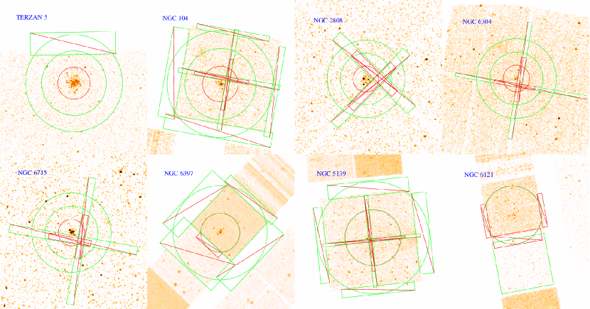
Figure 1.— Examples of GCs with large source extraction regions. We defined for each GCs the source region ($S_{h}$) as a (red) circle with radii of $r_{h}$, while defined the background region as a (green) annulus with inner-to-outer radii of $2r_{h}-3r_{h}$. Regions near CCD edges or gaps (rectangles with red diagonal lines) are masked to minimize uncertainty in the detector response. For GCs with a large $r_{h}$, the background annulus was set as $r_{h}-2r_{h}$ and from the same CCDs as for the source region; the only exception is NGC 6121, where the background region was chosen from the S2 CCD (green rectangle in the lower right panel). We adopted a ‘double subtraction’ procedure to correct for the vignetting effect for these GCs (see text for details).

Since the Chandra field-of-view (FoV) is not always large enough to cover the half-light circle (Figure 1), we defined for each observation a correction parameter $k_{1}=S_{h}/{S_{\rm FoV}}$, where $S_{h}=\pi r_{h}^{2}$ and $S_{\rm FoV}\leq S_{h}$ is the actual area allowed by the FoV. In this regard, the total flux is calculated as $F_{\rm X}=k_{1}\times F_{\rm X,FoV}$, where $F_{\rm X,FoV}$ is the flux within $S_{\rm FoV}$.

For the background region, we adopted an annulus with inner-to-outer radii of $2r_{h}-3r_{h}$ when the FoV was large enough, but for those GCs with a large $r_{h}$, the annulus was set as $r_{h}-2r_{h}$. We required that the background region fall within the same CCDs (AICS-I or ACIS-S3) as of the cluster region, but for NGC 6121, the background was chosen from ACIS-S2. We also avoided CCD edges and gaps where detector response may have a substantial uncertainty. We defined for each observation a second parameter $k_{2}=S_{\rm FoV}/{B_{\rm FoV}}$, where $B_{\rm FoV}$ is the actual background area allowed by the FoV (Figure 1). In most cases, $k_{2}$ was less than $0.5$ (Table 2).

Next, we calculated for each observation the cluster net counts as $N_{S}-N_{B}^{\prime}=N_{S}-k_{2}N_{B}$, where $N_{S}$ and $N_{B}$ are the 0.5–8 keV counts within $S_{\rm FoV}$ and $B_{\rm FoV}$, respectively. The signal-to-noise ratio, $S/N=(N_{S}-N_{B}^{\prime})/\sqrt{N_{S}+N_{B}^{\prime}}$, was derived for each observation and listed in Table 4. Among the 69 GCs, 51 have $S/N\geq 3$ and are considered as solid detections.

For most of our sample GCs, the total X-ray luminosity is not expected to be dominated by any single source. However, a source caught in a rare outburst may affect the total X-ray luminosity substantially. Therefore, for each observation we ran the CIAO wavdetect script to detect sources. A source located in $S_{\rm FoV}$ was referred to as an outbursting source if its 0.5-8 keV unabsorbed luminosity, derived with a power-law spectral model, is greater than $3\times 10^{33}{\rm~{}erg~{}s^{-1}}$. Such bright sources, found in only 3 GCs (Table 3), in which they each contribute more than $70\%$ of the total net count rate, were subsequently removed for flux calculation.

Spectra were then extracted from the cluster and background regions for each GC. The background-subtracted cluster spectra were grouped to have at least 20 counts and a minimum signal-to-noise ratio of 3 per bin. We performed spectral analysis with Xspec v12.8.0. The models adopted to fit the spectra were either an absorbed power-law (phabs*powerlaw), an absorbed bremsstrahlung (pabs*brem), or a combination of the two (phabs*(powerlaw+brem)). We calculated the absorption column density ($N_{\rm H}$) of each GC from their color excess $E(B-V)$ and fixed this parameter in the fit. If a GC had more than one observations, a joint fit was performed to minimize the statistical uncertainty, allowing the normalization to vary but having the other parameters linked among the observations. The 0.5–8 keV unabsorbed flux was derived from the best-fit model. For the 18 GCs with $S/N<3$, we derived for them an upper limit in the net count rate (at $95\%$ confidence) using the CIAO tool aprates, and converted it into an unabsorbed flux assuming an intrinsic power-law model with the photon-index fixed at $2.0$. We then calculated the 0.5–8 keV luminosity or upper limit by adopting the cluster distance from Harris (2010 edition). Our spectral analysis results are summarized in Table 4.

Direct subtraction of the local background is expected to be a sufficient treatment for most GCs. For 13 GCs with a relatively large angular extent ($r_{h}\gtrsim 2^{\prime}$; marked by “*” in Table 4), however, the effect of vignetting may bias low the background level, which is necessarily estimated at large off-axis angles. For such GCs, we corrected for vignetting following the ‘double-subtraction’ procedure (e.g., Li et al. 2011): a first subtraction of the non-vignetted instrumental background followed by a second subtraction of the vignetted cosmic background. Briefly, we first generated the instrumental background spectra for both the cluster and background regions, using the Chandra “stowed” background files. We then characterized the local cosmic background spectrum (i.e., instrumental background-subtracted) with a phenomenological model, being either an absorbed power-law or a power-law plus APEC thermal plasma with absorption. The hence derived cosmic background was added as a fixed component to the total spectral model, after scaling with the sky area.

Lastly, we examined the effect of source variability on the derived total X-ray luminosity, focusing on three GCs (Terzan 5, NGC 6626 and NGC 6397) with multiple observations. The spectra extracted from individual observations were fitted independently with an absorbed power-law model. The results, listed in Table 5, indicate that in all three cases the derived X-ray luminosity varies by less than $30\%$ over a timespan of years. This mild variability should have little effect on our statistical analysis and conclusions below.

2.3. 2MASS Data

To obtain an accurate measurement of the X-ray emissivity, a well determined cluster stellar mass is required. We adopted the K-band image of the Two Micron All Sky Survey (2MASS; Jarrett et al. 2000), which is expected to be a better proxy of old stellar populations in GCs than the optical bands such as those quoted in Harris (2010 edition). We downloaded the archival 2MASS images of the individual GCs and derived their K-band luminosity, $L_{K}$, as follows. The cluster and background regions for photometry were the same as those used in the X-ray analysis (Section 2.2). If a single 2MASS image did not cover the defined regions, we calibrated several adjacent images and merged them into a mosaic image with astrometry correction. We then obtained the K-band apparent magnitude of the cluster region after subtracting the background and correcting for extinction with $E(B-V)$. Finally, we calculated $L_{K}$ according to the apparent magnitude and cluster distance, which is expressed in units of solar K-band luminosity $L_{K,\odot}=5.67\times 10^{31}$ $\rm erg\,s^{-1}$ (for solar K-band absolute magnitude $M_{K,\odot}=+3.31$). The results are listed in Table 4.

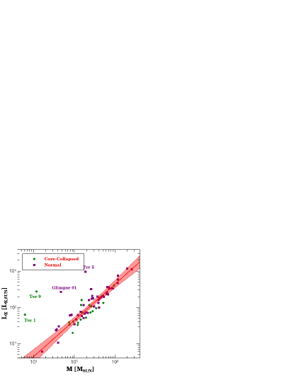
Figure 2.— GC K-band luminosity versus cluster mass $M$, which is derived from V-band magnitude following the empirical relation of Ma et al. (2015). The olive dots and purple squares donate the core-collapsed and dynamically normal GCs, respectively. The red line is the best-fit function, with shaded area representing the $95\%$ confidence range. The four outliers are marked.

To establish the use of $L_{K}$ as a proxy of the cluster mass $M$, we first calculated $M$ using the V-band magnitude listed in Harris (2010 edition), following the empirical relation by Ma et al. (2015), $M/{\rm M_{\odot}}=10^{-0.4(M_{V}-5.764\pm 0.063)}$, which is based on multi-band photometry of 297 GCs in M 31 and stellar population synthesis models. Figure 2 shows that $L_{K}$ is tightly correlated with $M$. Most GCs follow a fitted power-law function $L_{K}/L_{K,\odot}=10^{-0.38\pm 0.23}\times{(M/{\rm M_{\odot}})}^{1.00\pm 0.04}$, which suggests a quasi-linear relation between $L_{K}$ and $M$.

In the above fit, we have excluded four significant outliers (Terzan1, Terzan 5, Terzan 9 and Glimpse 01). We note that all these four GCs suffer from strong foreground extinction, thus their V-band fluxes may have been underestimated. For example, the V-band magnitude-based masses of Terzan 5 and Glimpse 01 are $1.88\times 10^{5}{\rm M_{\odot}}$ and $4.67\times 10^{4}{\rm M_{\odot}}$, respectively, whereas their K-band luminosities, $9.67\times 10^{5}L_{K,\odot}$ and $2.41\times 10^{5}L_{K,\odot}$, predict $\sim$12 times larger masses according to the above $L_{K}-M$ relation. Hereafter, we adopt a cluster mass of $2\times 10^{6}{\rm~{}M_{\odot}}$ for Terzan 5 and $3\times 10^{5}{\rm~{}M_{\odot}}$ for Glimpse 01, which were obtained by Lanzoni et al. (2010) and Pooley et al. (2007), respectively, and are consistent with our $L_{K}-M$ relation. Because there is no reliable source of cluster mass for Terzan 1 and Terzan 9, we do not include these two core-collapsed clusters in the following statistical analysis.

3. Statistical relations

As discussed in Section 1, in the absence of luminous LMXBs, the bulk of X-ray emission from GCs arises from a collection of CVs, ABs, qLMXBs and MSPs, hence the cumulative X-ray luminosity ($L_{X}$) should be roughly scaled with the total number of such sources, and more fundamentally, scaled with the cluster mass ($M$). If dynamical interactions are prone to create X-ray sources, a correlation between $L_{X}$ and the stellar encounter rate ($\Gamma$) is also expected. Other physical properties, such as metallicity, stellar density, age and structural parameters, of the GCs may also affect the formation and evolution of the X-ray populations. In this section, we examine the dependence of the cumulative X-ray emissivity, and hence the source abundance, on the various cluster properties. We define the cumulative X-ray emissivity as $\epsilon_{X}=2L_{X}/M$, where the factor of 2 accounts for the fact that $L_{X}$ as given in Table 4 has been measured within the half-light circle. The quasi-linear $L_{K}-M$ relation derived in Section 2.3 also allows us to adopt the quantity $L_{X}/L_{K}$ as a proxy of the X-ray emissivity, which has the virtue of being distance-independent. The GC parameters are taken from Harris (2010 edition); errors, when available and relevant, are also quoted.

3.1. Correlations with cluster mass

In Figure 3, we plot $L_{X}$ versus $L_{K}$ for all GCs. A correlation between $L_{X}$ and $L_{K}$ is evident, for which we find the Spearman’s rank correlation coefficient $r=0.694\pm 0.078$, with the p-value of $7.4\times 10^{-11}$ for random correlation. We fit a power-law function to the correlation and obtain $L_{X}\propto L_{K}^{0.74\pm 0.13}$, which is marked by the red solid line in Figure 3. Here and below we exclude the GCs with $S/N<3$ (highlighted with open symbols in the figures) from the fit to the correlations. There is no significant difference between the dynamically normal and core-collapsed GCs. A power-law fitting function for the dynamically normal GCs gives $L_{X}\propto L_{K}^{0.79\pm 0.12}$ (purple line in Figure 3). Notably, the fitted indice imply a sub-linear correlation.

Figure 3.— GC X-ray luminosity as a function of the K-band luminosity. The olive circles and purple squares donate the core-collapsed and dynamically normal GCs. Filled and open symbols represent the luminosity and upper limit, respectively. The solid lines mark the best-fitting functions, purple for the dynamically normal GCs and red for the full sample, respectively. The shaded area represents the $95\%$ confidence range.

In Figure 4, we plot the GC X-ray emissivity $\epsilon_{X}$ versus $M$. Here the latter has been derived from $M/{\rm M_{\odot}}=10^{0.38}\times(L_{K}/L_{K,\odot})$ rather than the V-band magnitude-based masses (Section 2.2). It can be seen that $\epsilon_{X}$ has a substantial scatter ranging from $10^{27}$ to a few times $10^{28}\rm\ erg\ s^{-1}{\rm M^{-1}_{\odot}}$. Nevertheless, a marginally significant negative correlation between $\epsilon_{X}$ and $M$ for the full sample is suggested by the Spearman’s rank correlation coefficient $r=-0.323\pm 0.077$, with $p=0.007$ for random correlation. The best fitting power-law function is $\epsilon_{X}\propto M^{-0.30\pm 0.11}$ (red solid line in Figure 4). However, if NGC 6397 and NGC 5139 (labelled in Figure 4) are not included in the fit, the $\sim$ $3\,\sigma$ anti-correlation becomes $\sim$ $2\,\sigma$, with $\epsilon_{X}\propto M^{-0.19\pm 0.10}$. We note that this anti-correlation is consistent with the sub-linear correlations found in Figure 3.

Figure 4.— X-ray emissivity as a function of the cluster mass, which is derived from the best-fit $L_{K}-M$ relation shown in Figure 2. The olive circles and purple squares denote the core-collapsed and dynamically normal GCs. Filled and open symbols represent the measured X-ray emissivity and upper limit, respectively. The red solid line delineates the best-fitting function, with shaded area represents the $95\%$ confidence range, while the dashed line represents the mean X-ray emissivity of the full sample (dispersions marked by the pair of dashed lines). For comparison, the cumulative X-ray emissivities of CVs and ABs in the Solar vicinity (Sazonov et al., 2006; Revnivtsev et al., 2007) and of the Local Group dwarf elliptical galaxies (Ge et al., 2015) are marked by the blue and magenta strips, respectively. Two Galactic old open clusters from van den Berg et al. (2013) are marked by blue diamonds, which were not included in the fit. See text for details.

We also measure the average X-ray emissivity of all 67 GCs to be $(6.9\pm 2.6)\times 10^{27}\rm\ erg\,s^{-1}M^{-1}_{\odot}$, as marked in Figure 4 by the dashed horizantal lines. If only GCs with $S/N\geq 3$ were considered, the average emissivity is $(7.4\pm 2.8)\times 10^{27}\rm\ erg\,s^{-1}M^{-1}_{\odot}$. If the three outburst sources were taken back into account, the X-ray emissivity of their host GCs would increase substantially (Table 3), but they have little effect in the average GC emissivity, which becomes $(7.6\pm 2.7)\times 10^{27}\rm\ erg\,s^{-1}M^{-1}_{\odot}$. The average X-ray emissivities of the core-collapsed and dynamically normal GCs are marginally consistent with each other ($9.4\pm 3.4$ versus $6.2\pm 2.3\times 10^{27}\rm\ erg\,s^{-1}M^{-1}_{\odot}$).

For comparison, also shown as a blue strip in Figure 4 is the cumulative X-ray emissivity of CVs and ABs detected in the Solar neighborhood, with a value of $\epsilon_{X}=(11.7\pm 3.1)\times 10^{27}\rm\ erg\,s^{-1}M^{-1}_{\odot}$, which was based on the X-ray luminosity function of CVs and ABs with $L_{X}$ ranging from $10^{27}$ to $10^{34}\rm\ erg\,s^{-1}$(Sazonov et al., 2006). Also compared in Figure 4 (magenta strip) is the average stellar X-ray emissivity of four gas-poor dwarf elliptical galaxies (M 32, NGC 147, NGC 185 and NGC 205), with a value of $\epsilon_{X}=(11.9\pm 2.7)\times 10^{27}\rm\ erg\,s^{-1}M^{-1}_{\odot}$ derived from Ge et al. (2015). In their work, discrete sources with X-ray luminosities greater than $\sim$ $10^{34}\rm\ erg\,s^{-1}$ have been removed to ensure that the unresolved X-ray emission from these galaxies is dominated by CVs and ABs. We note that the Solar neighborhood and the dwarf elliptical galaxies exhibit highly similar stellar X-ray emissivities, indicating a quasi-universal emissivity in normal galactic environments, i.e., where stellar dynamical effects are not important (Ge et al., 2015). On the other hand, as clearly shown in Figure 4, most GCs have a cumulative X-ray emissivity lower than the field level represented by the Solar neighborhood and the dwarf ellipticals. This strongly suggests a dearth rather than over-abundance of weak X-ray sources in GCs relative to the field .

For completeness, we place in Figure 4 two old open clusters, M 67 and NGC 6981. Their cumulative X-ray emissivities, derived from van den Berg et al. (2013), are significantly higher than that of most GCs and the field. Such a trend was previously noted by Verbunt (2001) based on ROSAT observations, and by Ge et al. (2015) based on only four GCs observed by Chandra.

3.2. Correlations with stellar encounter rate

Traditionally, the stellar encounter rate, $\Gamma\propto\int{\rho}^{2}/\sigma$, has been evaluated as $\Gamma\propto\rho_{c}^{2}r_{c}^{3}/\sigma_{c}$ or $\Gamma\propto\rho_{c}^{1.5}r_{c}^{2}$ (Verbunt & Hut, 1987; Verbunt, 2003), with the assumption that the spatial distribution of stars in GCs can be characterized by the King model (King, 1962, 1966). Here $r_{c}$ is the core radius and $\rho_{c}$ the average stellar density within $r_{c}$. The central velocity dispersion follows $\sigma_{c}\propto\rho_{c}^{0.5}r_{c}$ for a virial system.

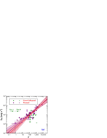
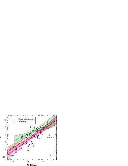
Figure 5.— (a) GC X-ray luminosity as a function of the stellar encounter rate. (b) The stellar encounter rate versus cluster mass $M$. Color-coded symbols denote the different types of GCs as in Figure 3. Solid lines and the associated shaded area are the power-law fitting functions and the $95\%$ confidence range, purple for the dynamically normal GCs, olive for the core-collapsed GCs and red for the full sample. The two outliers, Terzan 1 and Terzan 9, were not included in the fit.

To quantify the dynamical interactions in GCs, we adopt the updated stellar encounter rates by Bahramian et al. (2013). These authors have reconstructed the stellar density profiles of GCs based on their surface brightness profiles, thus the dynamically normal and core-collapsed GCs can be treated equally. More importantly, with Monte-Carlo simulations, errors in $\Gamma$ can also be properly estimated from the uncertainty in the observables such as distance, reddening and surface brightness. Specifically, we adopt $\Gamma_{1}\propto 4\pi\sigma_{c}^{-1}\int\rho^{2}(r)r^{2}dr$ from Table 4 of Bahramian et al. (2013), which is integrated over the entire cluster and normalized to a value of 1000 for NGC 104, and is compatible to our measurement of the X-ray luminosity.

In Figure 5a, we plot $L_{X}$ as a function of $\Gamma$ for each GC. It is evident that a strong correlation between $L_{X}$ and $\Gamma$ exists for the dynamically normal GCs. The Spearman’s rank correlation coefficient is $r=0.769\pm 0.093$, with the p-value of $p=1.7\times 10^{-10}$ for random correlation. This correlation is still significant when taking the core-collapsed GCs into account, with $r=0.627\pm 0.078$ and $p=1.4\times 10^{-8}$ for the total GCs. The best fitting functions for the dynamically normal and total GCs can be written as $L_{X}\propto\Gamma^{0.62\pm 0.06}$ and $L_{X}\propto\Gamma^{0.67\pm 0.07}$, respectively (purple and red lines in Figure 5a). These relations are consistent with the finding of Pooley et al. (2003) that, above a limiting luminosity of $4\times 10^{30}\rm\ erg\ s^{-1}$, the number of detected X-ray sources in 12 GCs is proportional to the encounter rate, with $N_{X}\propto\Gamma^{0.74\pm 0.36}$. A similar result has been obtained by Maxwell et al. (2012), with $N_{X}\propto\Gamma^{0.55\pm 0.09}$ again based on only 12 GCs.

The core-collapsed GCs show no significant correlation among themselves, but notably many of them are located below the best-fitting correlation for the dynamically normal GCs. This is contrary to the work of Pooley et al. (2003), Lugger et al. (2007) and Maxwell et al. (2012), in which most core-collapsed GCs appeared abundant in X-ray sources and were located above the best-fitting correlation in their $N_{X}-\Gamma$ diagram. We suggest that this discrepancy is most likely due to their different adoption of $\Gamma$, which, based on the tranditional method, might have been underestimated for core-collapsed GCs. This is hinted in Figure 5b, in which $\Gamma$ from Bahramian et al. (2013) is plotted against $M$. Evidently, most core-collapsed GCs have a larger $\Gamma$ than the dynamically normal GCs at a given cluster mass. With this updated $\Gamma$, Bahramian et al. (2013) first noted the lower abundance of X-ray sources in core-collapsed GCs than in their dynamically normal counterparts, which is consistent with our results in Figure 5a.

The two significant outliers in the $L_{X}-\Gamma$ diagram, Terzan 1 and Terzan 9, deserve some remarks. Both show an X-ray luminosity significantly higher than expected from their $\Gamma$. Cackett et al. (2006) detected 14 X-ray sources in the central 1.4 arcmin of Terzan 1, about 20 times larger than expected from the $N_{X}-\Gamma$ relation of Pooley et al. (2003). For Terzan 9, with the 15.2 ks Chandra observation, we detected 4 X-ray sources within the half-light radius, also more than expected from the $N_{X}-\Gamma$ relation. As noted in Section 2.3, at face value the K-band luminosities of these two clusters are not compatible with their V-band magnitudes, which are likely due to strong foreground extinction. Therefore $\Gamma$, evaluated based on V-band data in Bahramian et al. (2013), might have been underestimated for both clusters, and it is premature to claim an over-abundance of X-ray sources in these two clusters.

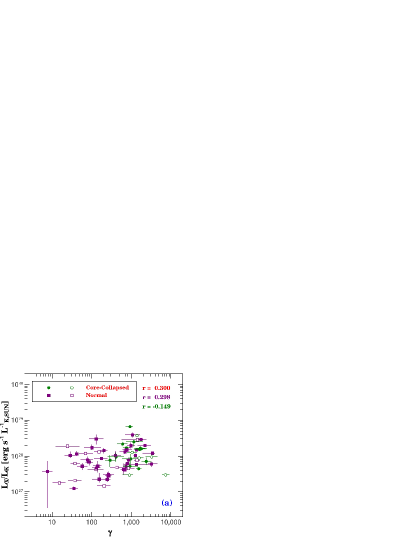
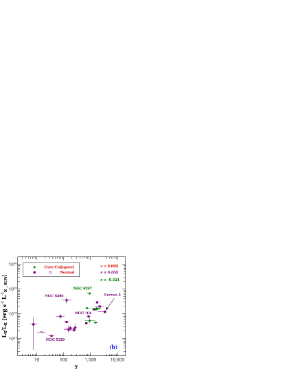
Figure 6.— $L_{X}/L_{K}$ as a function of the specific encounter rate $\gamma$ for (a) all the 69 GCs cosidered in this work, and (b) the 23 GCs considered in Pooley & Hut (2006). Color coded symbols denote different types of GCs as in Figure 3. Some well-studied GCs are marked with their names.

Now it becomes clear that $L_{X}$ depends on both $M$ and $\Gamma$, and so does $N_{X}$, the number of detected X-ray sources in a given GC. To minimize the dependence on cluster mass, Pooley & Hut (2006) and Pooley (2010) have studied the specific number of detected sources ($n_{x}\equiv N_{X}/M_{6}$) as a function of the specific encounter rate ($\gamma\equiv\Gamma/M_{6}$), where $M_{6}$ is the cluster mass in units of $10^{6}{\rm M_{\odot}}$. Pooley & Hut (2006) found that the two parameters are correlated, with a fitting function $n_{x}=C+A\gamma^{\alpha}$, where $C$, $A$, and $\alpha$ are free parameters. In this regard, the origin of X-ray sources in GCs can be attributed to two channels: descendants of primordial binaries ($C$) and a dynamically formed population ($A\gamma^{\alpha}$).

Similarly, we plot $L_{X}/L_{K}$ versus $\gamma$ in Figure 6, showing all 69 GCs in Figure 6a, but only those 23 GCs considered by Pooley & Hut (2006) in Figure 6b to facilitate a direct comparision. Since $\Gamma$ were estimated based on the V-band data by Bahramian et al. (2013), here we have calculated $\gamma$ ($\gamma\equiv\Gamma/M_{6}$) using the V-band-based mass (Figure 2) for consistency. Both Figure 2d of Pooley & Hut (2006) and our Figure 6b show a moderate increase of X-ray source abundance (in terms of $n_{x}$ or $L_{X}/L_{K}$) with increasing $\gamma$. However, the much larger sample in Figure 6a does not support a significant correlation; the Spearman’s rank correlation coefficients for the dynamically normal, core-collapse and total GCs are $r=0.298\pm 0.092$, $r=-0.149\pm 0.149$ and $r=0.300\pm 0.078$, with random correlation p-value of $p=0.040$, $p=0.542$ and $p=0.013$, respectively.

We end this subsection by emphasizing that a significant correlation exists between $\Gamma$ and $M$ (Figure 5b). The Spearman’s rank coefficients for the dynamically normal, core-collapsed and total GCs are $r=0.754\pm 0.092$, $0.660\pm 0.149$ and $0.611\pm 0.078$, respectively, with the p-value of $5.365\times 10^{-11}$, $0.002$ and $8.543\times 10^{-8}$ for random correlation. We fit the $\Gamma-M$ correlation with a power law function, which gives $\Gamma\propto M^{1.43\pm 0.17}$ for dynamically normal GCs, $\Gamma\propto M^{1.01\pm 0.26}$ for core-collapsed GCs, and $\Gamma\propto M^{1.28\pm 0.17}$ for total GCs. The fitting functions are also plotted in Figure 5b.

3.3. Correlations with other physical parameters

Observationally, LMXBs are more likely to be found in old, metal-rich GCs, rather than in young, metal-poor ones (Bellazzini et al., 1995; Kundu et al., 2002; Sarazini et al., 2003; Kim et al., 2006; Sivakoff et al., 2007; Li et al., 2010; Paolillo et al., 2011; Kim et al., 2013). This indicates that the formation and evolution of LMXBs in GCs are affected by stellar metallicity. It has been suggested that a smaller convection zone in metal-poor stars relative to metal-rich stars at a given mass may help turn off the magnetic braking during binary evolution, leading to a lower formation efficiency of LMXBs in metal-poor GCs (Ivanova, 2006). Alternatively, a stronger irradiation-induced wind from metal-poor stars, due to less efficient line cooling and energy dissipation, will speed up the evolution of LMXBs in the host cluster and reduce their number (Maccarone et al., 2004).

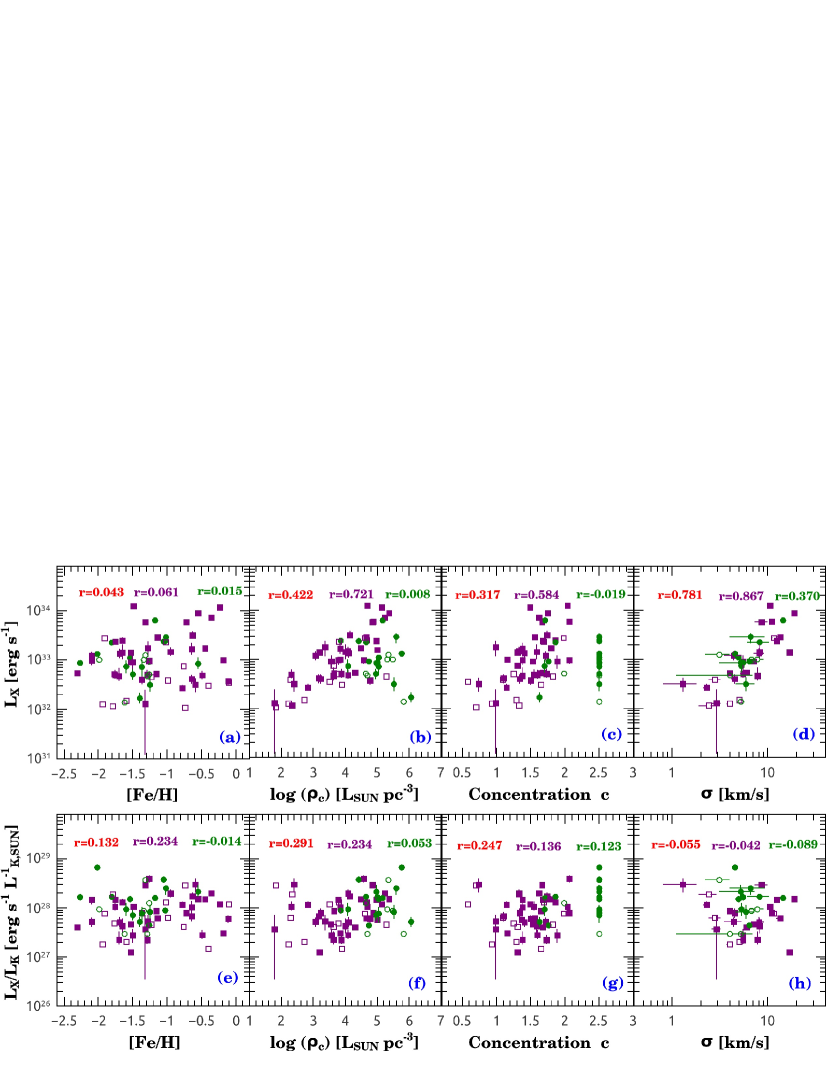
Figure 7.— Dependence of the X-ray luminosity (top panels) and $L_{X}/L_{K}$, a proxy of the X-ray emissivity (bottom panels), on various physical properties of GCs. From left to right: Metallicity, central luminosity density, King model central concentaration and central velocity dispersion. All these parameters are adopted from Harris (2010 edition). Color-coded symbols represent the different types of GCs as in Figure 3, and same color-coded text give the Speraman rank correlation coefficients: olive for core-collapsed, purple for dynamically normal and red for the total.

In Figure 7a and 7e, we test the dependence of $L_{X}$ and $L_{X}/L_{K}$ on metallicity. No clear correlation exists for these quantities. Presumably the same physical processes such as magnetic braking and irradiation also happen in CVs and ABs, but the influence of metallicity in these processes appears less important than in the case of LMXBs.

In Figure 7b, we study the dependence of $L_{X}$ on the cluster central luminosity density $\rho_{c}$. It is evident that the dynamically normal GCs have a larger $L_{X}$ with increasing $\rho_{c}$. The core-collapsed GCs have higher central stellar densities, but they exhibit no similar correlation between $L_{X}$ and $\rho_{c}$. On the other hand, dependence of $L_{X}/L_{K}$ on $\rho_{c}$ is not evident in Figure 7f for either the dynamically normal or core-collapsed GCs. This suggests that cluster mass is the more fundamental parameter underlying the $L_{X}-\rho_{c}$ relation.

In Figure 7c and 7d, a positive correlation exists between $L_{X}$ and the cluster central concentration $c$ or the central velocity dispersion $\sigma$. We note that similar relations between GC V-band absolute magnitude and $c$ or $\sigma$ have been found by Djorgovski & Meylan (1994). These two correlations may again reflect the more fundamental dependency on cluster mass. Indeed, Figure 7g and 7h show no significant correlation between $L_{X}/L_{K}$ and $c$ or between $L_{X}/L_{K}$ and $\sigma$.

In Figure 8a-d, we plot $L_{X}/L_{K}$ as a function of GC core relaxation time $t_{c}$, median relaxation time $t_{h}$, relative age $t_{r}$ and absolute age $t_{a}$. In general, GCs with smaller $t_{c}$ or $t_{h}$ are dynamically older. It appears that the GC X-ray emissivity increases with the dynamical age, as suggested by a marginally significant negative dependence of $L_{X}/L_{K}$ on $t_{c}$ and $t_{h}$ (Figure 8a and 8b, respectively). The marginal dependence of $L_{X}/L_{K}$ on the relative age $t_{r}$ or the absolute age $t_{a}$ (Figure 8c and 8d) is also consistent with such a mild trend.

In Figure 8e-g, we plot $L_{X}/L_{K}$ as a function of the GC distance to the Galactic center $R_{gc}$, ellipticity of optical isophotes $e$, tidal radius $r_{t}$ and main sequence binary fraction $f_{b}$. In principle, with increasing distances away from the Galactic center, GCs will suffer from weaker tidal force and grow their tidal radius, affecting its dynamical and geometrical structure and potentially the abundance of binaries. This is suggested by the mild anti-correlations in Figure 8e and 8g. However, we find no statistically significant correlation between $L_{X}/L_{K}$ and ellipticity of optical isophotes $e$ in Figure 8f. Although the main sequence binary fraction ($f_{b}$) may be closely related to the abundance of the weak X-ray sources, Figure 8h shows no significant correlation between $L_{X}/L_{K}$ and $f_{b}$.

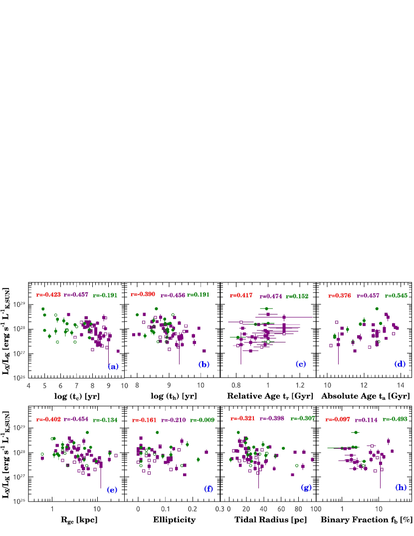
Figure 8.— Dependence of $L_{X}/L_{K}$, a proxy of the X-ray emissivity on various global properties of GCs. Top panels from left to right: Cluster core relaxation time, median relaxation time, relative age and absolute age. Bottom panels from left to right: Cluster distance to Galactic center, ellipticity of optical isophotes, tidal radius and main sequence binary fraction. All these parameters are adopted from Harris (2010 edition), except that the cluster relative age is from Marín-Franch et al. (2009), absolute age from Forbes & Bridges (2010) and the main sequence binary fraction from Milone et al. (2012). Color-coded symbols and text have the same meanings as in Figure 7.

To conclude this section, we summarize in Table 6 the Spearman’s rank coefficients for all the tested correlations.

4. Discussion

It has been known for over 40 years that the abundance of luminous LMXBs in GCs exceeds that of the field by orders of magnitude, which is generally accepted as the consequence of efficient dynamical formation of neutron star binaries in the dense environment of GCs. Hut & Verbunt (1983) were among the first to predict that dynamical processes would lead to the formation of as many white dwarf binaries as neutron star binaries in GCs. Pooley and colleagues, upon finding a correlation between the number of weak X-ray sources and the stellar encounter rate for a moderate sample of GCs, argued that the X-ray populations, in particular CVs, are over-abundant in GCs. Our analysis in Section 3, however, points to an opposite trend: most GCs exhibit a lower cumulative X-ray emissivity than found in the field, which is represented by the Solar neighborhood and the Local Group dwarf elliptical galaxies. Because in all these environments the cumulative X-ray emissivity is a reasonable proxy of the source abundance, the immediate conclusion is that the weak X-ray populations, primarily CVs and ABs, are under-abundant in GCs as compared to the field. In the following, we address the implications of this result.

4.1. Dependence on stellar encounter rate

The under-abundance of weak X-ray sources in GCs demands for a revisit of the $N_{X}-\Gamma$ (Pooley et al., 2003) and $L_{X}-\Gamma$ (Figure 5a) correlations as evidence for a predominantly dynamical origin of the X-ray populations. As shown in Figure 5b, the stellar encounter rate $\Gamma$ is strongly correlated with the cluster mass $M$, thus it is not unreasonable to raise the question of whether cluster mass is the more fundamental parameter underlying the $N_{X}-\Gamma$ and $L_{X}-\Gamma$ relations. Indeed, in Section 3.1 we have demonstrated a correlation between $L_{X}$ and $L_{K}$ (hence $M$), which is statistically as significant as the $L_{X}-\Gamma$ relation, according to the Spearman’s rank cofficients. Moreover, our larger GC sample disfavors a strong positive correlation between the source abundance (traced by $L_{X}/L_{K}$) and the specific encounter rate, $\gamma$ (Figure 6a), as previously suggested by Pooley & Hut (2006).

To further compare the influence of the cluster mass and stellar encounters on the X-ray populations, we test a correlation between $L_{X}$, $M$ and $\Gamma$ using the following form: ${\rm log}\ L_{X}=a_{K}\,{\rm log}\ L_{K}+a_{\Gamma}\,{\rm log}\ \Gamma+c$. Giving equal weights to $L_{K}$ and $\Gamma$ in the regression, we find $a_{K}=0.64\pm 0.12$, $a_{\Gamma}=0.19\pm 0.07$ and $c=29.4\pm 0.52$ (Figure 9). It appears that the cluster mass, rather than the stellar encounter rate, is the predominant factor in determining the amount of weak X-ray sources. This implies that a substantial fraction of the X-ray populations, in particular CVs and ABs, are descendants of primordial binaries, although dynamical processes must have played at least a partial role in the formation of the X-ray populations. In any case, taking the $N_{X}-\Gamma$ and $L_{X}-\Gamma$ relations as solid evidence for a dynamical origin of the X-ray populations may be an over-simplification. Below, we argue that not all dynamical interactions in GCs will lead to the formation of X-ray sources.

Figure 9.— GC X-ray luminosity expressed as a function of K-band luminosity and stellar encounter rate: The olive dots and purple squares donate the core-collapsed and dynamically normal GCs, respectively.

4.2. Efficiency of the primordial channel of close binary formation

In general, when considering the formation of close binary systems in a dense stellar environment such as GCs, three competing and coupled effects are relevant. The first is normal stellar evolution that eventually turns wide, primordial binaries into close binaries, which is referred to as the primordial channel. The second is the dynamical formation of close binaries due to two-body or three-body interactions. The third and a negative effect is the dynamical disruption of primordial binaries mainly due to three-body (binary-single) or four-body (binary-binary) interactions (Heggie, 1975; Hills, 1975; Mikkola, 1983; Hut et al., 1992a, b; Hut, 1993; Bacon et al., 1996). For LMXBs, because of the rarity of neutron stars and the relatively short lifetime of their progenitor stars, the first and third effects are generally negligible. However, for CVs and ABs, because their progenitors are mainly low-mass stars, they should evolve on a timescale comparable to or even greater than the GC relaxation time, making all the above three effects relevant. Therefore, we argue that the under-abundance of CVs and ABs in GCs reflects a low efficiency of the primordial channel, i.e., a substantial fraction of the primordial binaries are dynamically disrupted before they can otherwise evolve into close binaries. Such a scenario is supported by both theoretical and observational studies.

Theoretically, the fate of binaries in GCs is governed by both normal stellar evolution and stellar dynamical interactions. In the former case, a number of stellar processes, such as Roche lobe msss tranfer, steller wind and supernova kick, can substantially modify the binary oribits and even lead to orbit disruption or binary merger. Dynamical interactions can alter binaries in a more abrupt manner. For example, most “soft” binaries in GCs will be destroyed if they suffer from a strong encounter with other stars. Even for the “hard” binaries, their interactions with other stars can exchange one of the primordial members with the intruding star, in the meantime causing the orbit to expand or shrink, modifying the orbit eccentricity, enhancing the systemic velocity via gravitational recoil, or leading to physical collision. Numerical simulations have confirmed that binaries can be dynamically disrupted in GCs (Ivanova et al., 2005; Fregeau, 2009; Chatterjee et al., 2010). The probability for a primordial binary to survive from dynamical destruction depends on the binary hardness and the collision timescale in GCs. Comparing with simulations that only consider normal stellar evolution, simulations taking into account binary destruction result in a much lower binary fraction in GCs (Ivanova, 2011).

Observationally, the main sequence binary fraction is found to be on average much lower in GCs than in the Solar neighborhood (Cote et al., 1996; Albrow et al., 2001; Davis et al., 2008) or open clusters (Sollima et al., 2010). Recent numerical simulations suggest that these present-day binary fractions are consistent with a universal, near-unity initial binary fraction in GCs (Leigh et al., 2015). If this were the case, dynamical disruption of primordial binaries must have been efficient. This is also suggested by the observed trend that the main sequence binary fraction of GCs decreases with increasing cluster age (Sollima et al., 2007; Milone et al., 2012; Ji & Bregman, 2015). Furthemore, as shown in Figure 10, a negative correlation is evident between the main sequence binary fraction and the specific stellar encounter rate, strongly suggesting dynamical disruption of primordial binaries and consequently the dearth of X-ray-emitting close binaries.

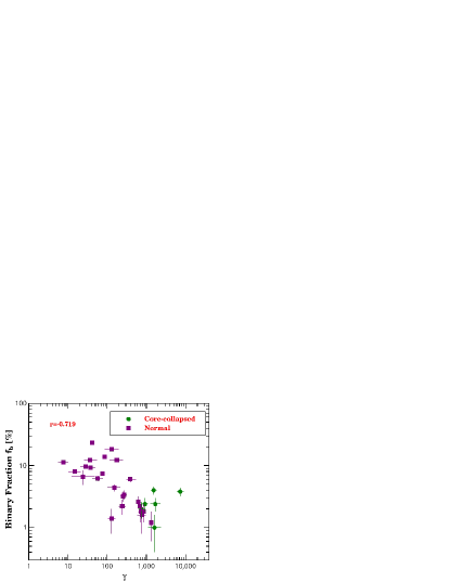
Figure 10.— Main sequence binary fraction of GCs (Milone et al., 2012) as a function of the specific encounter rate $\gamma$. The olive dots and purple squares donate the core-collapsed and normal GCs, respectively. The Spearman’s rank correlation coefficient is marked in red text.

4.3. Dynamical formation versus dynamical disruption

Nevertheless, dynamical formation of CVs and ABs must be taking place in GCs. In reality, it is most likely that dynamical formation and destruction of binaries occur simultaneously and persistently in GCs. Fortunately, the two competing effects may be unified in one process, namely, the binary-single interaction. In general, such interactions obey the Hills-Heggie law, which states that hard binaries (with $|E_{b}|>E_{k}$) evolve into smaller orbits, while soft binaries (with $|E_{b}|<E_{k}$) tend to be softer and even disrupted (Hills, 1975; Heggie, 1975).

More quantitatively, we may express the abundance of X-ray binaries as,

$$L_{X}/L_{K}\approx N_{X}\bar{L}_{X}/(N_{*}\bar{L}_{K})=(N_{b}/N_{*})(N_{X}/N_{b})\bar{L}_{X}/\bar{L}_{K},$$ (1)

where $\bar{L}_{X}$ ($\bar{L}_{K}$) is the characteristic X-ray (K-band) luminosity of a binary (star), $N_{b}/N_{*}\approx f_{b}$ is the GC binary fraction, and $N_{X}/N_{b}$ is the fraction of binaries being an X-ray-emitting close binary. Recall that the average GC X-ray emissivity is $\sim$40% lower than that of the cumulative X-ray emissivity of the field populations ($6.9\times 10^{27}\rm\ erg\,s^{-1}M^{-1}_{\odot}$ vs. $11.8\times 10^{27}\rm\ erg\,s^{-1}M^{-1}_{\odot}$; Section 3.1). On the other hand, the main sequence binary fraction in the Solar neighborhood is $\sim$40% (Fischer & Marcy, 1992), while most measurements of GC binary fraction range between 1-20% (Figure 7h).

If we assume that GCs have an initial binary fraction at least comparable to that of the Solar neighborhood – in fact, a near-unity initial binary fraction has been suggested for GCs (Leigh et al. 2015) – and that the Solar neighborhood binaries had evolved little due to the lack of dynamical interactions, from the above we may infer that the reduction in binary fraction (by a factor of 2-40 in $N_{b}/N_{*}$) due to dynamical disruption of “soft” primordial binaries has been partially compensated by the dynamical formation of X-ray-emitting “hard” binaries (i.e., an enhanced $N_{X}/N_{b}$ as compared to the field). The statistical outcome of this competition appears to be a mild anti-correlation between the abundance of the X-ray sources and the cluster mass, $\epsilon_{X}\propto M^{-0.31\pm 0.09}$ (Section 3.1), which may be qualitatively understood in the sense that dynamical disruption of primordial binaries is more efficient in more massive GCs, because of their higher encounter rate ($\Gamma\propto M^{1.28}$ in Figure 5b) and higher stellar velocity dispersion ($E_{k}\propto\sigma^{2}$). On the other hand, the competition may allow the abundance of weak X-ray sources in some dynamically old GCs to catch up with, or even exceeds, the field level. For example, NGC 6397 has the highest X-ray emissivity among all GCs (Figures 4 and 5), and the binary fraction in this cluster is also very low ($f_{b}=2.4\pm 0.6\%$, Milone et al. 2012), which suggests that the compensation of weak X-ray sources by dynamical formation channel have surpassed the dynamical disruption channel, and many “hard” main sequence binaries have been dynamically transformed into weak X-ray sources in this cluster. We leave a more quantitative study of the effect of binary-single interaction on the X-ray source abundance to a future work.

5. Summary

In this work, we have surveyed the cumulative X-ray emission of the largest-so-far sample (69) of Milky Way globular clusters observed by Chandra. Our main findings are as follows.

1. The X-ray emissivity of most GCs is lower than that of the Solar neighborhood and dwarf elliptical galaxies, indicating that a paucity of weak X-ray sources, mainly CVs and ABs, in GCs with respect to the field populations. This under-abundance of X-ray-emitting close binaries suggests that formation of such systems through the primordial channel is suppressed in GCs, which is likely due to dynamical disruption of primordial binaries before they can evolve into CVs and ABs.

2. The GC X-ray luminosity, stellar encounter rate and cluster mass are highly correlated among each other, with $L_{X}\propto\Gamma^{0.67\pm 0.07}$, $L_{X}\propto M^{0.74\pm 0.13}$ and $\Gamma\propto M^{1.28\pm 0.17}$. Furthermore, the GC X-ray luminosity can be expressed as a function of cluster mass and stellar encounter rate, with ${\rm Log}\ L_{X}=(29.40\pm 0.47)+(0.64\pm 0.12)\ {\rm Log}\ L_{K}+(0.19\pm 0.07)\ {\rm Log}\ \Gamma$, which suggests that dynamical formation of CVs and ABs in GCs is less dominant than previously thought, while the primordial channel may still have a substantial contribution.

3. Binary-single interactions, which would lead to both the disruption of soft primordial binaries and the formation of close binaries, seem to provide a natural explanation of the above results. The net outcome is the present-day abundance of weak X-ray sources in GCs, which appears no higher than that of the field.

4. Correlations between the GC X-ray emissivity and global cluster properties such as metallicity, dynamical age and structural parameters have been examined, but no statistically significant trends can be revealed.

Table 1BASIC PROPERTIES OF GLOBULAR CLUSTERS

Name	M	$\Gamma$	$-\delta$	$+\delta$	$\gamma$	$-\delta$	$+\delta$	D	E(B-V)	$r_{h}$	$r_{h}/r_{c}$	Fe/H	$\rho_{c}$	$t$
(1)	(2)	(3)	(4)	(5)	(6)	(7)	(8)	(9)	(10)	(11)	(12)	(13)	(14)	(15)
Normal GCs:
NGC 104	118.5	1000	134	154	844	113	130	4.5	0.04	3.17	8.8	-0.72	4.88	13.06
NGC 288	10.13	0.766	0.205	0.284	7.56	2.02	2.80	8.9	0.03	2.23	1.7	-1.32	1.78	10.62
NGC 2808	115.2	923	82.7	67.2	801	71.8	58.3	9.6	0.22	0.8	3.2	-1.14	4.66	10.8
NGC 3201	19.3	7.17	2.27	3.56	37.1	11.8	18.4	4.9	0.24	3.1	2.4	-1.59	2.71	10.24
NGC 5024	61.6	35.4	9.6	12.4	57.5	15.6	20.1	17.9	0.02	1.31	3.7	-2.1	3.07	12.67
NGC 5139	256.8	90.4	20.4	26.3	35.2	7.94	10.2	5.2	0.12	5	2.1	-1.53	3.15	11.52
NGC 5272	72.04	194	18	33.1	269	25	45.9	10.2	0.01	2.31	6.2	-1.5	3.57	11.39
NGC 5286	63.33	458	60.7	58.4	723	95.8	92.2	11.7	0.24	0.73	2.6	-1.69	4.1	12.54
NGC 5824	70.08	984	155	171	1400	221	244	32.1	0.13	0.45	7.5	-1.91	4.61	12.8
NGC 5904	67.55	164	30.4	38.6	243	45	57.1	7.5	0.03	1.77	4.0	-1.29	3.88	10.62
NGC 5927	26.89	68.2	10.3	12.7	254	38.3	47.2	7.7	0.45	1.1	2.6	-0.49	4.09	12.67
NGC 6093	39.59	532	68.8	59.1	1340	174	149	10	0.18	0.61	4.1	-1.75	4.79	12.54
NGC 6121	15.19	26.9	9.56	11.6	177	62.9	76.4	2.2	0.35	4.33	3.7	-1.16	3.64	12.54
NGC 6139	44.63	307	82.1	95.4	688	184	214	10.1	0.75	0.85	5.7	-1.65	4.67	–
NGC 6144	11.11	3.14	0.85	1.07	28.3	7.65	9.63	8.9	0.36	1.63	1.7	-1.76	2.31	13.82
NGC 6205	53.16	68.9	14.6	18.1	130	27.5	34	7.1	0.02	1.69	2.7	-1.53	3.55	11.65
NGC 6218	16.97	13.0	4.03	5.44	76.6	23.8	32.1	4.8	0.19	1.77	2.2	-1.37	3.23	12.67
NGC 6287	17.77	36.3	7.74	7.70	204	43.6	43.3	9.4	0.6	0.74	2.6	-2.1	3.78	13.57
NGC 6304	16.81	123	22	53.8	732	131	320	5.9	0.54	1.42	6.8	-0.45	4.49	13.57
NGC 6333	30.59	131	41.8	59.1	428	137	193	7.9	0.38	0.96	2.1	-1.77	3.78	–
NGC 6341	38.87	270	29	30.1	695	74.6	77.4	8.3	0.02	1.02	3.9	-2.31	4.3	13.18
NGC 6352	7.83	6.74	1.3	1.71	86.1	16.6	21.8	5.6	0.22	2.05	2.5	-0.64	3.17	12.67
NGC 6362	12.18	4.56	1.03	1.51	37.4	8.46	12.4	7.6	0.09	2.05	1.8	-0.99	2.29	13.57
NGC 6366	3.996	5.14	1.76	2.75	129	44	68.8	3.5	0.71	2.92	1.3	-0.59	2.39	13.31
NGC 6388	117.4	899	213	238	766	181	203	9.9	0.37	0.52	4.3	-0.55	5.37	12.03
NGC 6401	29.21	44	10.7	11	151	36.6	37.7	10.6	0.72	1.91	7.6	-1.02	3.79	–
NGC 6402	88.23	124	30.2	31.8	141	34.2	36	9.3	0.6	1.3	1.6	-1.28	3.36	–
NGC 6440	63.91	1400	477	628	2193	746	983	8.5	1.07	0.48	3.4	-0.36	5.24	–
NGC 6517	40.33	338	97.5	152	838	242	377	10.6	1.08	0.5	8.3	-1.23	5.29	–
NGC 6528	8.58	278	49.5	114	3240	577	1330	7.9	0.54	0.38	2.9	-0.11	4.77	–
NGC 6535	1.61	0.388	0.192	0.389	24.2	12	24.2	6.8	0.34	0.85	2.4	-1.79	2.34	10.5
NGC 6539	41.84	42.1	15.3	28.6	101	36.6	68.4	7.8	1.02	1.7	4.5	-0.63	4.15	–
NGC 6553	25.92	69	18.8	26.8	266	72.5	103	6	0.63	1.03	1.9	-0.18	3.84	–
NGC 6569	41.46	53.6	20.8	30.2	129	50.2	72.8	10.9	0.53	0.80	2.3	-0.76	3.63	–
NGC 6626	37.12	648	91.1	83.8	1750	245	226	5.5	0.4	1.97	8.2	-1.32	4.86	–
NGC 6637	22.99	89.9	18.1	36	391	78.7	157	8.8	0.18	0.84	2.5	-0.64	3.84	13.06
NGC 6638	14.24	137	27.1	38.6	962	190	271	9.4	0.41	0.51	2.3	-0.95	4.09	–
NGC 6656	50.77	77.5	25.9	31.9	153	51	62.8	3.2	0.34	3.36	2.5	-1.7	3.63	12.67
NGC 6715	198.4	2520	274	226	1273	138	114	26.5	0.15	0.82	9.1	-1.49	4.69	10.75
NGC 6717	3.71	39.8	13.7	21.8	1070	369	587	7.1	0.22	0.68	8.5	-1.26	4.58	13.18
NGC 6760	27.64	56.9	19.4	26.6	206	70.2	96.2	7.4	0.77	1.27	3.7	-0.4	3.89	–
NGC 6809	21.56	3.23	1	1.38	15	4.64	6.4	5.4	0.08	2.83	1.6	-1.94	2.22	12.29
NGC 6838	3.55	1.47	0.138	0.146	4.15	3.89	4.12	4	0.25	1.67	2.7	-0.78	2.83	13.7
NGC 7089	82.72	518	71.4	77.6	626	86.3	93.8	11.5	0.06	1.06	3.3	-1.65	4	11.78
Glim 01	30.00	400	200	200	8560	4280	12800	4.2	4.85	0.65	5.6	–	5.0	–
Pal 10	4.18	59	35.5	42.8	1410	848	1020	5.9	1.66	0.99	1.2	-0.1	3.51	–
Ter 3	1.71	1.18	0.37	0.65	68.9	21.4	38.1	8.2	0.73	1.25	1.1	-0.74	1.82	–
Ter 5	200.0	6800	3020	1040	36200	16100	5540	5.9	2.38	0.72	3.4	-0.23	5.14	–
Core Collapse GCs:
NGC 362	47.6	735	117	137	1540	246	288	8.6	0.05	0.82	4.6	-1.26	4.74	10.37
NGC 1904	28.16	116	44.7	67.6	412	159	240	12.9	0.01	0.65	4.1	-1.6	4.08	11.14
NGC 5946	15.05	134	44.6	33.6	890	296	223	10.6	0.54	0.89	11.1	-1.29	4.68	11.39
NGC 6256	14.64	169	60.4	119	1150	413	813	10.3	1.09	0.86	43	-1.02	5.59	–
NGC 6266	94.97	1670	569	709	1760	599	747	6.8	0.47	0.92	4.2	-1.18	5.16	11.78
NGC 6293	26.16	847	239	337	3240	914	1440	9.5	0.36	0.89	17.8	-1.99	5.31	–
NGC 6325	12.29	118	45.6	44.7	960	371	364	7.8	0.91	0.63	21	-1.25	5.52	–
NGC 6342	7.48	44.8	12.5	14.4	599	167	193	8.5	0.46	0.73	14.6	-0.55	4.97	12.03
NGC 6355	34.17	99.2	25.7	41.1	290	75.2	120	9.2	0.77	0.88	17.6	-1.37	5.04	–
NGC 6397	9.15	84.1	18.3	18.3	919	200	200	2.3	0.18	2.9	58	-2.02	5.76	12.67
NGC 6453	15.62	371	88.7	128	2380	568	820	11.6	0.64	0.44	8.8	-1.5	4.95	–
NGC 6522	23.21	363	98.5	113	1560	424	478	7.7	0.48	1	20	-1.34	5.48	–
NGC 6541	51.71	386	63.1	95.2	746	122	184	7.5	0.14	1.06	5.9	-1.81	4.65	12.93
NGC 6544	12.07	111	36.5	67.8	920	302	562	3	0.76	1.21	24.2	-1.4	6.06	10.37
NGC 6558	7.61	105	19.3	26.2	1380	253	344	7.4	0.44	2.15	71.7	-1.32	5.35	–
NGC 6642	9.32	97.8	24.5	31.3	1050	263	336	8.1	0.4	0.73	7.3	-1.26	4.64	–
NGC 6681	14.24	1040	192	267	7300	1350	1870	9	0.07	0.71	23.7	-1.62	5.82	12.8
NGC 6752	24.98	401	126	182	1610	504	729	4	0.04	1.91	11.24	-1.54	5.04	11.78
NGC 7099	19.3	324	81.2	124	1680	421	642	8.1	0.03	1.03	17.2	-2.27	5.01	12.93
Ter 1	1.17	0.292	0.17	0.274	24.9	14.5	23.3	6.7	1.99	1.4	95.5	-1.03	3.85	–
Ter 9	0.616	1.71	0.959	1.67	278	256	271	7.1	1.76	0.78	26	-1.05	4.42	–

Note. — Column 1-2: Name, total globular cluster mass (in units of $10^{4}M_{\odot}$) derived from V-band magnitude. Column 3-5: Stellar encounter rate from Bahramian et al. (2013), except for Glimpse 01, which is adopted from Pooley et al. (2007). $\pm\delta$ is the $1\sigma$ upper and lower limits of $\Gamma$. Column 6-8: specific encounter rate, which is calculated with $\gamma=\Gamma/M_{6}$, where $M_{6}$ is the GC mass in units of $10^{6}M_{\odot}$. Column 9-10: GC distance in units of kpc, foreground color excess. Column 11-12: half-light radius in arcmins, and ratio of half-light radius to core radius. Column 13-15: metallicity, central luminosity density in units of $log_{10}(L_{\odot}\rm\ pc^{-3})$ and absolute age of GCs in units of $\rm Gyr$ (Forbes & Bridges, 2010).

Table 2OBSERVATION LOG

GC Name	Chandra Obs.ID	Effect. exposure	Background	Cluster region	Source to Background
		$t_{exp}$(ks)	Region	factor $k_{1}$	region factor $k_{2}$
(1)	(2)	(3)	(4)	(5)	(6)
Normal GCs:
NGC 104	953, 955	30.7, 30.7	2, 2	1.21, 1.16	0.249, 0.252
NGC 288	3777	45.6	1	1.04	0.471
NGC 2808	7453, 8560	45.4, 10.8	2, 2	1.71, 1.71	0.148, 0.147
NGC 3201	11031	82.9	1	1	0.894
NGC 5024	6560	24.2	2	1	0.316
NGC 5139	13726, 13727	171, 47.6	1, 1	1.11, 1.10	0.440, 0.415
NGC 5272	4542, 4543, 4544	9.9, 9.8, 9.4	1, 1, 1	1.05, 1.05, 1.05	0.942, 0.890, 0.914
NGC 5286	8964, 9852	10, 3.3	2, 2	1, 1	0.232, 0.235
NGC 5824	9026	10.7	2	1	0.200
NGC 5904	2676	41.8	2	1	0.412
NGC 5927	13673, 8953	46.5, 0.77	2, 2	1, 1	0.276, 0.290
NGC 6093	1007	36.1	2	1	0.200
NGC 6121	946, 7446, 7447	25.2, 47.9, 44.8	1, 1, 1	1.21, 1.22, 1.21	0.811, 0.841, 0.825
NGC 6139	8965	17.7	2	1	0.260
NGC 6144	7458	53.4	2	1	0.330
NGC 6205	5436, 7290	26.5, 26.6	2, 2	1, 1	0.464
NGC 6218	4530	22.8	2	1	0.447
NGC 6287	13734	39.7	2	1	0.268
NGC 6304	11073, 8952	96.2, 4.9	2, 2	1.52, 1	0.143, 0.321
NGC 6333	8954	7.8	2	1	0.288
NGC 6341	5241, 3778	19.7, 29.3	2, 2	1, 1	0.246, 0.241
NGC 6352	13674	19.5	2	1	0.595
NGC 6362	11024, 12038	28.8, 8.7	1, 1	1, 1	0.411, 0.404
NGC 6366	2678	20.1	1	1	0.784
NGC 6388	5505	44.6	2	1	0.200
NGC 6401	8948	11.1	2	1.04	0.578
NGC 6402	8947	11.8	2	1	0.299
NGC 6440	947, 3799, 11802	22.6, 23.4, 4.91	2, 2, 2	1, 1, 1	0.200, 0.200, 0.200
NGC 6517	9597	23.3	2	1	0.200
NGC 6528	8961, 12400	12.2, 52.7	2, 2	1, 1	0.200, 0.200
NGC 6535	11025	52.4	2	1	0.200
NGC 6539	8949	14.4	2	1	0.440
NGC 6553	13671, 8957	30.9, 4.9	2, 2	1, 1	0.255, 0.285
NGC 6569	8974	11.1	2	1	0.245
NGC 6626	2683, 2684, 2685	8.9, 12.4, 12.5	2, 2, 2	1, 1, 1	0.632, 0.602, 0.606
	9132, 9133	141, 52.5	2, 2	1, 1	0.568, 0.561
NGC 6637	8946	7.4	2	1	0.253,
NGC 6638	8950	8.3	2	1	0.200
NGC 6656	5437, 14609	15.8, 84.6	1, 1	1.02, 1.26	1.219, 0.799
NGC 6715	4448	29.1	2	1.59	0.150
NGC 6717	13733	16.9	2	1	0.240
NGC 6760	13672	50.7	2	1	0.277
NGC 6809	4531	33.7	1	1.04	0.622
NGC 6838	5434	50.8	2	1	0.453
NGC 7089	8960	11.2	2	1	0.326
Glim 01	6587	44.6	2	1	0.200
Pal 10	8945	10.8	2	1	0.299
Ter 3	11026	64.3	2	1	0.231
Ter 5	13706,10059,13705	45.5, 35.9, 13.2	2, 2, 2	1, 1, 1	0.225, 0.244, 0.243
	14339,14625,15615	34.1, 48.9, 82.9	2, 2, 2	1, 1, 1	0.235, 0.262, 0.266
	3798,13225,13252	24.9, 29.7, 39.2	2, 2 ,2	1, 1, 1	0.200, 0.234, 0.241
	14475,14476,14477	29.3, 28.0, 28.3	2, 2, 2	1, 1, 1	0.426, 0.428, 0.428
	14478	28.3	2	1	0.449
Core Collapse GCs:
NGC 362	4529, 5229	51.1, 8	2, 2	1, 1	0.218, 0.218
NGC 1904	9027	10	2	1	0.200
NGC 5946	9956	24.3	1	1	0.349
NGC 6256	8951	9.4	2	1	0.268
NGC 6266	2677	60.7	2	1	0.200
NGC 6293	8962	9.6	2	1	0.271
NGC 6325	8959	16.7	2	1	0.237
NGC 6342	9957	15.8	2	1	0.236
NGC 6355	9958	22.2	2	1	0.274
NGC 6397	79, 2668, 2669	48.3, 28.1, 26.7	1, 1, 1	1.19, 1.04, 1.03	0.213, 0.708, 0.708
	7460, 7461	146, 88.9	1, 1	1.11, 1.10	0.596, 0.671
NGC 6453	9959	20.4	2	1	0.200
NGC 6522	8963	8.33	2	1	0.272
NGC 6541	3779	43.2	2	1	0.274
NGC 6544	5435	8.96	2	1	0.266
NGC 6558	9961	11	1	1.08	0.516
NGC 6642	8955	6.4	2	1	0.236
NGC 6681	9955, 8958	67.8, 6.9	2, 2	1, 1	0.233, 0.237
NGC 6752	948, 6612	27.5, 37	2, 2	1, 1	0.501, 0.585
NGC 7099	2679	43	2	1	0.217
Ter 1	5464	18.5	1	1.24	0.317
Ter 9	9960	15.2	2	1	0.239

Note. — Column 1-3: Name, Chandra observation ID and effective exposure time. Column 4: background regions, 1 and 2 denote the use of annulus with radii $r_{h}-2r_{h}$ and $2r_{h}-3r_{h}$, respectively. Column 5-6: value of $S_{h}/S_{fov}$ and $S_{fov}/B_{fov}$.

Table 3GCs with X-ray sources in outburst

Name	ID	$N_{s}-N_{b}^{\prime}$	$S1$	$L_{X,1}$	$L_{X}$	$L_{X,tot}$	$2L_{X,tot}/M$
(1)	(2)	(3)	(4)	(5)	(6)	(7)	(8)
NGC 5272	4542	419	297	$3.02^{+0.23}_{-0.26}$	$0.70^{+0.38}_{-0.26}$	$3.63^{+0.41}_{-0.30}$	$0.92^{+0.38}_{-0.33}$
	4543	750	628	$5.84^{+0.35}_{-0.62}$	$1.05^{+0.29}_{-0.29}$	$8.18^{+0.93}_{-0.80}$	$2.07^{+0.86}_{-0.89}$
NGC 6717	13733	865	643	$5.49^{+0.23}_{-0.56}$	$0.97^{+0.14}_{-0.15}$	$5.82^{+0.35}_{-0.41}$	$19.8^{+9.08}_{-9.28}$
NGC 6453	9959	286	255	$3.17^{+0.32}_{-0.28}$	$0.46^{+0.13}_{-0.10}$	$3.41^{+0.29}_{-0.37}$	$4.37^{+0.37}_{-0.47}$

Note. — Column 1-2: Cluster name, Chandra observation ID. Column 3-4: Cluster net counts and counts of the outburst source. Column 5-8: Luminosities (0.5-8 keV) of the outburst source, GC cumulative luminosity when the outburst source has been rejected and included separatively, with a units of $10^{33}\rm\ erg\ s^{-1}$. Column 9: The total X-ray emissivity of GCs in units of $10^{28}\rm\ erg\ s^{-1}M_{\odot}^{-1}$.

Table 4DERIVED X-RAY PROPERTIES

Name	Net counts	S/N	Model	nH	PI	KT	$\chi^{2}_{\nu}$	$L_{X,0.5-8}$	$L_{K}$	$L_{X}/L_{K}$
(1)	(2)	(3)	(4)	(5)	(6)	(7)	(8)	(9)	(10)	(11)
Normal GCs:
NGC 104∗	17246	102.5	PL+Brem	0.023	$0.42^{+0.04}_{-0.05}$	$0.65^{+0.05}_{-0.08}$	376.3/352	$58.9^{+7.65}_{-8.56}$	74.6	$7.90^{+1.03}_{-1.15}$
NGC 2808	700	19.2	PL	0.128	$1.92^{+0.16}_{-0.16}$		21.3/38	$28.9^{+2.53}_{-1.86}$	46.91	$6.16^{+0.54}_{-0.40}$
NGC 288∗	230	3.2	PL	0.017	$2.15^{+1.72}_{-1.51}$		42.8/22	$1.28^{+1.19}_{-1.16}$	3.42	$3.74^{+3.48}_{-3.40}$
NGC 3201	93	0.48	PL	0.139	$2$(frozen)			$<1.49$	7.21	$<2.07$
NGC 5024	184	4.2	PL	0.012	$2$(frozen)		3.8/3	$12.1^{+2.56}_{-2.59}$	23.1	$5.24^{+1.11}_{-1.12}$
NGC 5139∗	12012	32.4	PL+Brem	0.069	$1.52^{+0.16}_{-0.14}$	$0.21^{+0.07}_{-0.08}$	171.3/167	$14.1^{+1.56}_{-1.09}$	112.2	$1.26^{+0.14}_{-0.10}$
NGC 5272∗	365	5.1	PL	0.006	$2.34^{+0.81}_{-0.64}$		58.9/46	$9.14^{+3.09}_{-2.63}$	32.98	$2.77^{+0.94}_{-0.80}$
NGC 5286	134	6.1	PL	0.139	$2.1^{+0.52}_{-0.49}$		2.8/8	$13.5^{+3.55}_{-2.6}$	26.1	$5.17^{+1.36}_{-0.99}$
NGC 5824	14	1.2	PL	0.075	$2.0$(frozen)			$<27.8$	35.98	$<7.73$
NGC 5904	513	6.9	PL	0.017	$1.8^{+0.42}_{-0.41}$		9.5/10	$5.06^{+1.37}_{-0.83}$	22.75	$2.22^{+0.60}_{-0.37}$
NGC 5927	330	6.0	PL	0.261	$2.0^{+0.58}_{-0.47}$		9.4/10	$4.86^{+1.23}_{-0.83}$	17.25	$2.82^{+0.71}_{-0.48}$
NGC 6093	960	23.3	PL	0.104	$1.78^{+0.12}_{-0.11}$		44.4/52	$23.7^{+1.39}_{-1.81}$	16.05	$14.8^{+0.87}_{-1.13}$
NGC 6121∗	3791	12.2	PL+Brem	0.203	$0.60^{+0.43}_{-0.73}$	$0.73^{+0.72}_{-0.30}$	385.3/279	$5.26^{+0.03}_{-0.70}$	6.14	$8.56^{+0.05}_{-1.14}$
NGC 6139	288	9.1	PL	0.435	$2.30^{+0.37}_{-0.34}$		9.3/13	$24.9^{+3.88}_{-3.48}$	18.87	$13.2^{+2.06}_{-1.84}$
NGC 6144	428	4.9	PL	0.209	$3.2$		11.7/6	$4.95^{+1.35}_{-0.81}$	4.67	$10.6^{+2.89}_{-1.73}$
NGC 6205	1373	15.0	PL	0.012	$2.14^{+0.17}_{-0.17}$		50.4/51	$9.15^{+0.62}_{-0.68}$	19.4	$4.72^{+0.32}_{-0.35}$
NGC 6218	380	6.3	PL	0.11	$1.55^{+0.51}_{-0.49}$		5.3/7	$4.01^{+0.97}_{-0.81}$	5.1	$7.87^{+1.90}_{-1.59}$
NGC 6287	232	6.9	PL	0.348	$1.15^{+0.41}_{-0.41}$		5.4/9	$9.75^{+1.61}_{-1.93}$	6.68	$14.6^{+2.41}_{-2.89}$
NGC 6304	1561	18.4	PL	0.313	$3.2^{+0.22}_{-0.21}$		57.7/56	$17.2^{+0.9}_{-0.6}$	11.55	$14.9^{+0.78}_{-0.52}$
NGC 6333	23	1.1	PL	0.22	$2.0$(frozen)			$<5.14$	10.58	$<4.86$
NGC 6341	643	12.4	PL	0.012	$2.16^{+0.22}_{-0.22}$		48.4/30	$5.42^{+0.51}_{-0.46}$	13.23	$4.10^{+0.38}_{-0.34}$
NGC 6352∗	337	5.4	PL	0.128	$3.17^{+0.65}_{-0.69}$		35.1/25	$4.14^{+0.84}_{-0.87}$	6.07	$6.82^{+1.38}_{-1.43}$
NGC 6362	106	1.1	PL	0.052	$2.0$(frozen)			$<3.88$	6.14	$<6.32$
NGC 6366∗	445	4.9	PL	0.412	$1.93^{+0.64}_{-0.63}$		68.6/57	$3.17^{+1.04}_{-0.98}$	1.06	$30.0^{+9.84}_{-9.28}$
NGC 6388	3682	54.9	PL	0.215	$2.05^{+0.05}_{-0.05}$		176.2/136	$88.8^{+1.67}_{-2.80}$	58.38	$15.2^{+0.29}_{-0.48}$
NGC 6401	74	1.5	PL	0.418	$2.0$(frozen)			$<23.2$	17.58	$<13.2$
NGC 6402	125	3.7	PL	0.348	$0.99^{+0.9}_{-0.93}$		1.44/3	$17.7^{+6.38}_{-6.11}$	33.16	$5.34^{+1.92}_{-1.84}$
NGC 6440	2672	46.9	PL	0.621	$2.78^{+0.08}_{-0.08}$		133/122	$72.5^{+1.73}_{-2.11}$	36.51	$19.9^{+0.47}_{-0.58}$
NGC 6517	17	0.9	PL	0.626	$2.0$(frozen)			$<4.53$	9.82	$<4.61$
NGC 6528	262	8.7	PL	0.313	$1.98^{+0.33}_{-0.31}$		7.1/14	$3.73^{+0.59}_{-0.69}$	6.23	$5.99^{+0.95}_{-1.11}$
NGC 6535	30	0.7	PL	0.197	$2.0$(frozen)			$<1.15$	0.607	$<19.0$
NGC 6539	333	6.8	PL	0.592	$3.37^{+0.69}_{-0.65}$		10.3/11	$31.7^{+6.41}_{-4.41}$	18.34	$17.3^{+3.49}_{-2.40}$
NGC 6553	627	12.4	PL	0.365	$2.88^{+0.32}_{-0.31}$		25.9/26	$9.96^{+1.03}_{-0.63}$	32.1	$3.10^{+0.32}_{-0.20}$
NGC 6569	18	0.8	PL	0.307	$2.0$(frozen)			$<7.58$	18.17	$<4.17$
NGC 6626	37119	123.4	PL	0.232	$1.98^{+0.03}_{-0.03}$		1135.5/658	$58.3^{+0.58}_{-0.53}$	19.75	$29.5^{+0.29}_{-0.27}$
NGC 6637	99	4.8	PL	0.104	$1.0^{+0.53}_{-0.49}$		4.7/5	$16.6^{+5.57}_{-3.74}$	15.98	$10.4^{+3.49}_{-2.34}$
NGC 6638	90	5.7	PL	0.238	$1.35^{+0.52}_{-0.48}$		1.24/6	$14.7^{+3.39}_{-2.44}$	7.51	$19.6^{+4.51}_{-3.25}$
NGC 6656∗	3629	17.6	PL	0.197	$1.66^{+0.69}_{-0.34}$		223.5/155	$4.70^{+2.18}_{-0.96}$	20.81	$2.26^{+1.05}_{-0.46}$
NGC 6715	271	11.6	PL	0.087	$2.38^{+0.24}_{-0.23}$		18.04/15	$124^{+12.5}_{-7.08}$	117.3	$10.6^{+1.07}_{-0.61}$
NGC 6717	221	8.9	PL	0.128	$0.99^{+0.33}_{-0.32}$		1.49/10	$9.67^{+1.48}_{-1.51}$	2.45	$39.4^{+6.04}_{-6.16}$
NGC 6760	85	1.5	PL	0.447	$2.0$(frozen)			$<3.03$	20.63	$<1.47$
NGC 6809	10	0.09	PL	0.046	$2.0$(frozen)			$<1.26$	7.02	$<1.80$
NGC 6838	1063	12.9	PL	0.145	$1.97^{+0.29}_{-0.28}$		15/18	$2.67^{+0.51}_{-0.36}$	2.33	$11.5^{+2.19}_{-1.55}$
NGC 7089	101	3.8	PL	0.035	$1.54^{+0.54}_{-0.48}$		3.1/5	$14.2^{+6.37}_{-4.01}$	33.16	$4.28^{+1.92}_{-1.21}$
Glim 01	1107	25.3	PL	2.813	$1.58^{+0.21}_{-0.21}$		65.9/48	$15.6^{+0.72}_{-0.97}$	26.98	$5.78^{+0.27}_{-0.36}$
Pal 10	15	0.7	PL	0.963	$2.0$(frozen)			$<3.54$	2.98	$<11.9$
Ter 3	-106	-1.5	PL	0.423	$2.0$(frozen)			$<1.07$	0.37	$<29.0$
Ter 5	39938	170.5	PL	1.380	$1.93^{+0.02}_{-0.02}$		2320.6/1687	$117^{+0.84}_{-1.13}$	96.65	$12.1^{+0.09}_{-0.12}$
Core Collapse GCs:
NGC 362	1368	26.3	Brem	0.029		$1.15^{+0.16}_{-0.13}$	62.7/61	$9.20^{+0.34}_{-0.46}$	20.63	$4.46^{+0.17}_{-0.22}$
NGC 1904	58	3.7	PL	0.006	$2.04^{+0.93}_{-0.72}$		1.7/4	$7.42^{+2.48}_{-2.01}$	7.83	$9.48^{+3.17}_{-2.57}$
NGC 5946	16	0.5	PL	0.313	$2.0$(frozen)			$<4.73$	15.94	$<2.97$
NGC 6256	135	6.1	PL	0.632	$1.81^{+0.51}_{-0.46}$		8.2/7	$29.4^{+4.3}_{-8.09}$	11.64	$25.3^{+3.69}_{-6.95}$
NGC 6266	5894	63.9	PL+Brem	0.273	$1.15^{+0.29}_{-0.36}$	$0.74^{+0.15}_{-0.13}$	238.6/176	$63.9^{+1.02}_{-4.99}$	39.86	$16.0^{+0.27}_{-1.25}$
NGC 6293	49	2.1	PL	0.209	$2.0$(frozen)		0/1	$<10.1$	10.67	$<9.47$
NGC 6325	82	4.1	PL	0.528	$2.0$(frozen)		3.06/2	$3.17^{+1.18}_{-0.90}$	3.79	$8.36^{+3.11}_{-2.37}$
NGC 6342	84	3.5	PL	0.267	$0.97^{+0.66}_{-0.61}$		1.5/4	$8.47^{+2.97}_{-1.87}$	3.9	$21.7^{+7.62}_{-4.80}$
NGC 6355	108	3.2	PL	0.447	$1.70^{+1.10}_{-0.84}$		0.34/3	$7.28^{+2.77}_{-2.56}$	9.47	$7.69^{+2.92}_{-2.70}$
NGC 6397∗	58210	133.5	PL+Brem	0.104	$1.19^{+0.02}_{-0.02}$	$0.29^{+0.08}_{-0.07}$	1315/1274	$13.3^{+0.48}_{-0.47}$	1.98	$67.3^{+2.41}_{-2.38}$
NGC 6453	284	12.2	PL	0.371	$2.0$(frozen)		3.2/3	$5.13^{+1.41}_{-1.14}$	7.2	$7.13^{+1.96}_{-1.58}$
NGC 6522	64	2.5	PL	0.278	$2.0$(frozen)			$<10.1$	11.48	$<8.8$
NGC 6541	2870	39.5	PL	0.081		$1.43^{+0.13}_{-0.11}$	139.3/103	$22.6^{+0.07}_{-0.08}$	13.28	$17.0^{+0.50}_{-0.59}$
NGC 6544	132	4.2	PL	0.441	$2.0$(frozen)		3.67/3	$1.71^{+0.44}_{-0.38}$	3.28	$5.21^{+1.35}_{-1.15}$
NGC 6558	87	1.6	PL	0.255	$2.0$(frozen)			$<12.62$	3.35	$<37.6$
NGC 6642	19	1.2	PL	0.232	$2.0$(frozen)			$<5.17$	4.06	$<12.7$
NGC 6681	72	1.4	PL	0.041	$2.0$(frozen)			$<1.38$	4.62	$<2.99$
NGC 6752	4640	35.4	PL	0.023	$1.47^{+0.06}_{-0.06}$		221.7/153	$11.1^{+0.38}_{-0.42}$	7.25	$15.3^{+0.52}_{-0.58}$
NGC 7099	1045	18.0	PL	0.017	$2.32^{+0.12}_{-0.12}$		68.2/50	$8.71^{+0.60}_{-0.56}$	5.22	$16.7^{+1.15}_{-1.07}$
Ter 1	633	12.2	PL	1.154	$1.41^{+0.33}_{-0.32}$		18.5/19	$24.5^{+2.12}_{-3.06}$	27.34	$8.96^{+0.77}_{-1.12}$
Ter 9	275	8.9	PL	1.021	$1.17^{+0.32}_{-0.34}$		8.9/13	$23.9^{+2.37}_{-3.06}$	6.26	$38.2^{+3.79}_{-4.89}$

Note. — Column 1-3: Name, observation net counts (0.5-8 keV) and signal-to-noise ratio. Column 4-5: X-ray spectral fitting model and the fixed absorption column in units of $10^{22}\rm\ cm^{-2}$, which is calculated with $N_{H}=0.58\times E(B-V)\times 10^{22}\rm\ {cm}^{-2}$. GCs marks with “*” have a large angular extent ($r_{h}\gtrsim 2^{\prime}$), we adopted the “Double Subtraction” procedure to correct the vignetting effect during spectral fitting. Column 6-8: Photon-index, plasma temperature in units of keV, and $\chi^{2}$/degree of freedom. Column 9-11: 0.5-8 keV X-ray luminosity of GCs in units of $10^{32}\rm\ erg\ s^{-1}$, K-band luminosity in units of $10^{4}L_{K,\odot}$ and X-ray to K-band luminosity ratio, in units of $10^{27}\rm\ erg\ s^{-1}L_{K,\odot}^{-1}$.

Table 5X-RAY VARIABILITY OF THREE GCs

Obs.ID	Exp.	Date	Model	nH	Photon		$\chi^{2}_{\nu}$	$L_{X}$
	(ks)			($10^{22}cm^{-2}$)	Index		(d.o.f.)	($10^{32}erg/s$)
Terzan 5:
3798	24.9	2003-07-13	PL	1.322	$1.82^{+0.08}_{-0.08}$		116.7/109	$137.3^{+3.85}_{-4.43}$
10059	35.9	2009-07-15	PL	1.322	$1.81^{+0.10}_{-0.09}$		129.3/135	$100.4^{+2.50}_{-3.13}$
13225	29.7	2011-02-17	PL	1.322	$1.99^{+0.09}_{-0.09}$		101.9/116	$119.2^{+3.62}_{-3.71}$
13252	39.2	2011-04-29	PL	1.322	$1.98^{+0.09}_{-0.08}$		151.2/122	$101.0^{+3.28}_{-3.59}$
13705	13.2	2011-09-05	PL	1.322	$1.99^{+0.14}_{-0.13}$		66.8/57	$116.0^{+4.67}_{-5.84}$
13706	45.5	2012-05-13	PL	1.322	$1.82^{+0.06}_{-0.06}$		202.9/187	$145.6^{+2.82}_{-3.17}$
14339	31.4	2011-09-08	PL	1.322	$1.98^{+0.09}_{-0.09}$		120.1/121	$111.7^{+2.61}_{-3.89}$
14475	29.3	2012-09-17	PL	1.322	$2.15^{+0.10}_{-0.10}$		111.2/105	$116.4^{+3.42}_{-3.54}$
14476	28.0	2012-10-28	PL	1.322	$2.03^{+0.10}_{-0.10}$		112.7/99	$110.2^{+4.01}_{-3.39}$
14477	28.3	2013-02-05	PL	1.322	$2.02^{+0.10}_{-0.10}$		117.9/100	$112.5^{+3.08}_{-5.12}$
14478	28.3	2013-07-16	PL	1.322	$1.88^{+0.09}_{-0.09}$		103.7/104	$115.4^{+3.83}_{-3.76}$
14625	48.9	2013-02-22	PL	1.322	$1.91^{+0.07}_{-0.07}$		229/175	$125.1^{+2.40}_{-2.49}$
15615	82.9	2013-02-23	PL	1.322	$1.88^{+0.05}_{-0.05}$		336.4/236	$113.1^{+1.72}_{-1.59}$
Joint	-	–	PL	0.232	$1.93^{+0.02}_{-0.02}$		2320.6/1687	$116.9^{+0.84}_{-1.13}$
NGC 6626:
2683	8.9	2002-09-09	PL	0.232	$2.03^{+0.15}_{-0.15}$		52.8/52	$45.3^{+2.11}_{-0.28}$
2684	12.4	2002-07-04	PL	0.232	$1.93^{+0.12}_{-0.12}$		59.3/65	$45.0^{+2.59}_{-1.61}$
2685	12.5	2002-08-04	PL	0.232	$2.14^{+0.14}_{-0.13}$		50.3/62	$38.4^{+2.28}_{-2.04}$
9132	141	2008-08-07	PL	0.232	$1.96^{+0.03}_{-0.03}$		339.5/296	$63.8^{+0.90}_{-0.82}$
9133	52.5	2008-08-10	PL	0.232	$2.00^{+0.06}_{-0.06}$		261/185	$58.8^{+1.17}_{-1.24}$
Joint	–	–	PL	0.232	$1.98^{+0.03}_{-0.03}$		1135.5/658	$58.3^{+0.58}_{-0.53}$
NGC 6397:
79	48.3	2000-07-31	PL	0.104	$1.42^{+0.04}_{-0.04}$		226.8/234	$16.0^{+0.28}_{-0.33}$
2668	28.1	2002-05-13	PL	0.104	$1.19^{+0.06}_{-0.06}$		202.4/202	$13.8^{+0.27}_{-0.37}$
2669	26.7	2002-05-15	PL	0.104	$1.21^{+0.07}_{-0.07}$		227.2/184	$11.4^{+0.37}_{-0.27}$
7460	146	2007-07-16	PL	0.104	$1.20^{+0.03}_{-0.03}$		302.3/335	$13.0^{+0.15}_{-0.16}$
7461	88.9	2007-06-22	PL	0.104	$1.14^{+0.03}_{-0.03}$		349.9/319	$15.9^{+0.31}_{-0.18}$

Note. — Column 1-3: Chandra observation ID, effective exposure time in units of keV and observation date. Column 4-6: X-ray spectral fitting model, the fixed absorption column in units of $10^{22}\rm\ cm^{-2}$ and Photon-index. Column 8-9: $\chi^{2}$/degree of freedom and GC 0.5-8 keV X-ray luminosity in units of $10^{32}\rm\ erg\ s^{-1}$.

Table 6TESTED CORRELATIONS

		Total GCs			Normal GCs			Core-Collapsed GCs
Relations		$r$	$p(>|r|)$		$r$	$p(>|r|)$		$r$	$p(>|r|)$
$L_{X}-L_{K}$		0.694	$7.2\times 10^{-11}$		0.754	$5.9\times 10^{-10}$		0.366	0.123
$L_{X}-\Gamma$		0.627	$1.4\times 10^{-8}$		0.769	$1.7\times 10^{-10}$		0.194	0.426
$\Gamma-M$		0.611	$4.1\times 10^{-8}$		0.754	$5.4\times 10^{-11}$		0.660	0.002
$\gamma-M$		0.111	0.374		0.337	0.019		0.125	0.611
$L_{X}/L_{K}-L_{K}$		-0.321	0.008		-0.272	0.061		-0.228	0.348
$L_{X}/L_{K}-\gamma$		0.300	0.013		0.298	0.040		-0.149	0.542
$L_{X}-Fe/H$		0.043	0.734		0.061	0.685		0.015	0.952
$L_{X}/L_{K}-Fe/H$		0.132	0.291		0.234	0.114		0.014	0.955
$L_{X}-\sigma$		0.781	$2.8\times 10^{-9}$		0.867	$2.0\times 10^{-8}$		0.370	0.174
$L_{X}/L_{K}-\sigma$		-0.055	0.737		-0.042	0.844		-0.089	0.751
$L_{X}-\rho$		0.422	$3.8\times 10^{-4}$		0.721	$7.2\times 10^{-9}$		0.008	0.974
$L_{X}/L_{K}-\rho$		0.291	0.017		0.234	0.109		0.053	0.830
$L_{X}-c$		0.317	0.009		0.584	$1.3\times 10^{-5}$		-0.019	0.938
$L_{X}/L_{K}-c$		0.247	0.044		0.138	0.358		0.123	0.615
$L_{X}-t_{c}$		-0.124	0.320		-0.331	0.023		0.184	0.450
$L_{X}/L_{K}-t_{c}$		-0.423	$4.0\times 10^{-4}$		-0.457	0.001		-0.191	0.432
$L_{X}-t_{h}$		0.270	0.027		0.238	0.103		0.542	0.016
$L_{X}/L_{K}-t_{h}$		-0.390	$1.1\times 10^{-3}$		-0.456	0.001		0.191	0.435
$L_{X}-t$		0.062	0.696		0.019	0.921		0.275	0.414
$L_{X}/L_{K}-t$		0.376	0.014		0.457	0.010		0.545	0.083
$L_{X}-t_{r}$		-0.021	0.906		0.014	0.942		-0.152	0.774
$L_{X}/L_{K}-t_{r}$		0.417	0.013		0.474	0.009		0.152	0.774
$L_{X}-r_{gc}$		-0.093	0.454		-0.117	0.426		-0.066	0.789
$L_{X}/L_{K}-r_{gc}$		-0.402	$7.5\times 10^{-4}$		-0.454	0.001		-0.134	0.587
$L_{X}-e$		-0.118	0.374		-0.058	0.713		-0.233	0.386
$L_{X}/L_{K}-e$		-0.161	0.222		-0.210	0.176		0.009	0.974
$L_{X}-r_{t}$		0.103	0.405		0.166	0.260		0.159	0.516
$L_{X}/L_{K}-r_{t}$		-0.321	0.008		-0.398	0.005		-0.307	0.201
$L_{X}-f_{b}$		-0.721	$6.9\times 10^{-6}$		-0.742	$3.3\times 10^{-5}$		-0.580	0.228
$L_{X}/L_{K}-f_{b}$		-0.097	0.609		0.114	0.597		-0.493	0.321

Note. — Spearman’s rank correlation test for each parameter. The $p(>|r|)$ values show the probability that a correlation arises randomly.

References

- Albrow et al. (2001) Albrow, M. D., Gilliland, R. L., Brown, T. M., Edmonds, P. D., et al. 2001, ApJ, 559, 1060
- Bacon et al. (1996) Bacon, D., Sigurdsson, S., Davis, M. B., 1996, MNRAS, 281, 830
- Bahramian et al. (2013) Bahramian, A., Heinke, C.O., Sivakoff, G.R., & Gladstone, J.C. 2013, ApJ, 766, 136
- Bellazzini et al. (1995) Bellazzini, M., Pasquali, A., Federici, L., et al. 1995, ApJ, 439, 687
- Cackett et al. (2006) Cackett, E. M., Wijnands, R., Heinke, C. O., Pooley, D., et al. 2006, MNRAS, 369, 407
- Chatterjee et al. (2010) Chatterjee, S., Fregeau, J. M., Umbreit, S., Rasio, F. A. 2010, ApJ, 719, 915
- Clark (1975) Clark, G. W. 1975, ApJ, 199, L143
- Cote et al. (1996) Cote, P., Fischer, P., 1996, AJ, 112,565
- Davis et al. (2008) Davis, D. S., Richer, H. B., Anderson, J., Brewer, J., et al. 2008, AJ, 135, 2141
- Djorgovski & Meylan (1994) Djorgovski, S., Meylan, G. 1994, ApJ, 108, 1292
- Edmonds et al. (2003) Edmonds, P. D., Gilliland, R. L., Heinke, C. O., & Grindlay, J. E. 2003, ApJ, 569, 1177
- Fabian et al. (1975) Fabian, A. C., Pringle, J. E., & Rees, M. J. 1975, MNRAS, 172, 15
- Fischer & Marcy (1992) Fischer, D. A., & Marcy, G. W. 1992, ApJ, 396, 178
- Forbes & Bridges (2010) Forbes, D. A., Bridges, T., 2010, MNRAS, 404,1203
- Fregeau et al. (2003) Fregeau, J. M. et al. 2003, ApJ, 593, 772
- Fregeau (2008) Fregeau, J. M. 2008, ApJ, 673, 25
- Fregeau (2009) Fregeau, J. M., Ivanova, N., Rasio, F. A. 2009, ApJ, 707, 1533
- Gao et al. (1991) Gao, B., Goodman, J., Cohn, H., Murphy, B. 1991, ApJ, 370, 567
- Ge et al. (2015) Ge, C., Li, Z-Y., Xue, X-J., Gu, Q-S., et al. 2015, ApJ, 812, 130
- Gnedin et al. (2002) Gnedin, O. Y., Zhao, H-S., et al. 2002, MNRAS, 568, 23
- Goodman & Hut (1989) Goodman, J., Hut, P. 1989, Nature, 339, 40
- Grindlay et al. (2001) Grindlay, J. E., Heinke, C. O., Edmonds, P. D., & Murray, S. S. 2001, science, 292, 2290
- Haggard et al. (2009) Haggard, D., Cool, A. M., & Davies, M. B. 2009, ApJ, 697, 224
- Harris (2010 edition) Harris, W. E. 1996(2010 edition), AJ, 112, 1487.
- Heggie (1975) Heggie, D. C., 1975, MNRAS, 173, 729
- Heinke (2011) Heinke, C. O. 2011, arXiv:astro-ph/1101.5356
- Heinke et al. (2003) Heinke, C. O., Grindlay, J. E., Lugger, P. M., et al. 2003, ApJ, 598, 501
- Heinke et al. (2005) Heinke, C. O., Grindlay, J. E., Cohn, H. N., et al. 2005, ApJ, 625, 796
- Heinke (2006) Heinke, C.O., Wijnands, R., Cohn,H.N., et al. 2006, ApJ, 651, 1098
- Hills (1975) Hills, J. G., 1975, AJ, 80, 809
- Hills (1976) Hills, J. G., 1976, MNRAS, 175, 1P
- Hut et al. (1992a) Hut, P., McMillan, S., Romani, R. W., 1992, ApJ, 389, 527
- Hut et al. (1992b) Hut, P., McMillan, S., Goodman, J., et al. 1992, PASP, 104, 981
- Hut (1993) Hut, P., 1993, ApJ, 403, 256
- Ivanova et al. (2005) Ivanova, N., Belczynski, K. Fregeau, J. M. and Rasio, F. A. 2005, MNRAS, 358, 572
- Ivanova (2006) Ivanova, N. 2006, ApJ, 636, 979
- Ivanova (2011) Ivanova, N. 2011, arXiv:astro-ph/1101.2684
- Jarrett et al. (2000) Jarrett, T. H., Chester, T., Cutri, R., et al. 2000, AJ, 119, 2498
- Ji & Bregman (2015) Ji, J., Bregman, J. N., 2015, ApJ, 807, 32
- Katz (1975) Katz, J. I. 1975, Nature, 253, 698
- Kim et al. (2006) Kim, E., Kim, D.-W., Fabbiano, G., et al. 2006, ApJ, 647, 276
- Kim et al. (2013) Kim, D. W., Fabbiano, N., Ivanova, Fragos, T., et al. 2013, ApJ, 764, 98
- King (1962) King, I. R. 1962, AJ, 67, 471
- King (1966) King, I. R. 1966, AJ, 71, 64
- Kundu et al. (2002) Kundu, A., Maccarone, T. J., & Zepf, S. E. 2002, ApJ, 574, 5
- Lanzoni et al. (2010) Lanzoni, B., Ferraro, F. R., Dalessandro, E., et al. 2010, ApJ, 717, 653
- Leigh et al. (2015) Leigh, N. W. C., Giersz, M., et al. 2015, MNRAS, 446, 226
- Li et al. (2010) Li, Z., Spitler, L. R., Jones, C., et al. 2010, ApJ, 721, 1368
- Li et al. (2011) Li, Z., Jones, C., Forman, W. R., et al. 2011, ApJ, 730, 84
- Liu et al. (2007) Liu, Q. Z., van Paradijs, J., & van den Heuvel, E. P. J., 2007, å, 469, 807
- Lugger et al. (2007) Lugger, P. M., Cohn, H. N., Heinke, C. O., et al. 2007, ApJ, 657, 286
- Maccarone et al. (2004) Maccarone, T. J., Kundu, A., Zepf, S. E. 2004, ApJ, 606, 430
- Ma et al. (2015) Ma, J., Wang, S., Wu, Z-Y., et al. 2015, AJ, 149, 56
- Marín-Franch et al. (2009) Marín-Franch, A., Aparicio, A., Piotto, G., et al. 2009, ApJ, 694, 1498
- Maxwell et al. (2012) Maxwell, J. E., Lugger, P. M., Cohn, H. N., et al. 2012, ApJ, 756, 147
- Mikkola (1983) Mikkola, S., 1983, MNRAS, 203, 1107
- Milone et al. (2012) Milone, A. P., Piotto, G., Bedin, L. R., et al. 2012, A&A, 540, 16
- Paolillo et al. (2011) Paolillo, M., Puzia, T. H., Goudfrooij, P., et al. 2011, ApJ, 736, 90
- Pooley et al. (2002a) Pooley, D., Lewin, W. H. G., Homer L., et al. 2002, ApJ, 569, 405
- Pooley et al. (2002b) Pooley, D., Lewin, W. H. G., Verbunt F., et al. 2002, ApJ, 573, 184
- Pooley et al. (2003) Pooley, D., et al. 2003, ApJ, 591, 131
- Townsley & Bildsten (2005) Townsley, D. M., Bildsten, L. 2005, ApJ, 628,395
- Pooley & Hut (2006) Pooley, D., & Hut, P. 2006, ApJ, 646, 143
- Pooley et al. (2007) Pooley, D., Rappaport, S., Levine, A., et al. 2007, arXiv: astro-ph/0708.3365
- Pooley (2010) Pooley, D. 2010, PNAS, 107, 7164
- Revnivtsev et al. (2007) Revnivtsev, M., Churazov, E., Sazonov, S., Forman, W., & Jones,C. 2007, A&A, 473, 783
- Sarazini et al. (2003) Sarazin, C. L., Kundu, A., Irwin, J. A., et al. 2003, ApJ, 595, 743
- Sazonov et al. (2006) Sazonov, S., Revnivtsev, M., Gilfanov, M., et al. 2006, A&A, 450, 117
- Sivakoff et al. (2007) Sivakoff, G. R., Jordan, A., Sarazin, C. L., et al. 2007, ApJ, 660, 1246
- Sollima et al. (2007) Sollima, A., Beccari, G., Ferraro, F. R., et al. 2007, MNRAS, 380, 781
- Sollima et al. (2010) Sollima, A., Carballo-Bello, J. A., Beccari, G., et al. 2010, MNRAS, 401, 577
- Sutantyo (1975) Sutantyo, W. 1975, A&A, 44, 227
- Townsley & Bildsten (2005) Townsley, D. M., & Bildsten, L. 2005, ApJ, 628, 395
- van den Berg et al. (2013) van den Berg, M., Verbunt, F., Tagliaferri, G., et al. 2013, ApJ, 770, 98
- Verbunt & Hut (1987) Verbunt, F., & Hut, P. 1987, in: The Origin and Evolution of Neutron Stars IAU Symp.125, eds. D.J. Helfand and J.H. Huang, Reidel, p.187
- Verbunt (2000) Verbunt, F. 2000, vol.198 of ASP Conf.Ser.,p.421
- Verbunt (2001) Verbunt, F. 2001, A&A, 368, 137
- Verbunt (2003) Verbunt, F. 2003, New Horizons in Globular Cluster Astronomy, ASP Conference Proceedings, Vol. 296, p. 245
- Verbunt & Freire (2014) Verbunt, F., Freire, P. C. C. 2014, A&A, 561, 11