Controllable single-photon nonreciprocal transmission in a cavity
optomechanical system with a weak coherent driving

Abstract

We study the nonreciprocal transmission of a single-photon in a cavity optomechanical system, in which the cavity supports a clockwise and a counter-clockwise circulating optical modes, the mechanical resonator (MR) is excited by a weak coherent driving, and the signal photon is made up of a sequence of pulses with exactly one photon per pulse. We find that, if the input state is a single-photon state, it is insufficient to study the nonreciprocity only from the perspective of the transmission spectrums, since the frequencies where the nonreciprocity happens are far away from the peak frequency of the single-photon. So we show the nonreciprocal transmission behavior by comparing the spectrums of the input and output fields. In our system, we can achieve a transformation of the signal transmission from unidirectional isolation to unidirectional amplification in the single-photon level by changing the amplitude of the weak coherent driving. The effects of the mechanical thermal noise on the single-photon nonreciprocal transmission are also discussed.

I Introduction

Nonreciprocal optical transmission has attracted more and more attention for its important potential applications in quantum information processing and quantum networks 1 . In the nonreciprocal optical devices, e.g., isolator, circulator, nonreciprocal phase shifter, unidirectional amplifier, the transmission of the information is not symmetric. Conventionally, the nonreciprocal transmission can be achieved by using the Faraday rotation effect in the magneto-optical crystals 2 ; 3 ; 4 ; 5 ; 6 ; 7 . However, this scheme requires large magnetic fields, and thus make it difficult to realize miniaturization and integration. In order to solve this problem, a number of schemes have been proposed to break the reciprocity without the use of magneto-optical effects. For example, one has proposed strategies that are based on the optical nonlinearity 8 , the spatial-symmetry-breaking structures 9 ; 10 ; 11 ; 12 , the indirect interband photonic transitions 13 ; 14 ; 15 ; 16 ; 17 ; 18 ; 19 , the optoacoustic effects 20 ; 21 , the parity-time-symmetric structures 22 ; 23 ; 24 ; 25 , and so on 26 ; 27 .

Recently, efforts have also been made to investigate the optical nonreciprocity in cavity optomechanical systems 28 ; 29 . Manipatruni et al. demonstrated that the optical nonreciprocal effect was based on the momentum difference between the forward and backward-moving light beams in a Fabry-Perot cavity with one moveable mirror 30 . Subsequently, Hafezi et al. proposed a scheme to achieve the nonreciprocal transmission in a microring resonator by using a unidirectional optical pump 31 . More recently, many theoretical works aiming at achieving the circulator 32 , the nonreciprocal quantum-state conversion 33 , and the unidirectional optical amplifier 34 have been proposed in various of cavity optomechanical systems. However, it is still a challenge to achieve the nonreciprocal transmission in the single-photon or few-photon level. At present, only a few works towards this target have been reported 31 ; 35 ; 36 .

In this paper, we study the nonreciprocal transmission of a single-photon in a cavity optomechanical system, as shown in Fig. 1, in which the cavity supports a clockwise and a counter-clockwise circulating optical modes, the mechanical resonator (MR) is excited by a weak coherent driving, and the signal photon is made up of a sequence of pulses with exactly one photon per pulse. We show that, it is insufficient to discuss the nonreciprocity from the perspective of the transmission spectrums when we consider a single-photon state as the input state, since the frequencies where the nonreciprocity happens are far away from the peak frequency of the single-photon. We will show the nonreciprocal transmission of the single-photon by comparing the spectrums of the input and output fields. In our system, we can achieve the unidirectional isolation and unidirectional amplification of the signal in the single-photon level. Essentially, this two kind of transmission behaviors are both caused by the unidirectional optical pump, and the switch from the isolation to the amplification depends on the amplitude of the weak coherent driving.

This paper is organized as follows. In Section II we introduce the theoretical model, calculate the Langevin equations, derive the expressions of the transmission spectrums and the spectrums of the output fields. In Section III, we analyze the cause and condition of the unidirectional isolation of the signal in the single-photon level by comparing the spectrums of the input and output fields. Next in Section IV, we use the same method to discuss the cause and condition of the unidirectional amplification of the signal. In Section V, we consider the affect of the mechanical noise on the nonreciprocal transmission, the experimental feasibility of our system is also discussed in this section. Finally, we provide a brief summary.

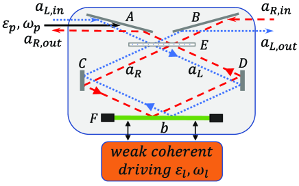
Figure 1: (color online) Schematic diagram of our proposed model. A, B, C, D are fixed mirrors of total reflection, E is a fixed mirrors of partial transmission, and F is a movable mirror (treated as a mechanical resonator, MR) of total reflection. C, D, E, and F constitute a ring resonator, which supports a clockwise and a counter-clockwise circulating optical modes. The MR is excited by a weak coherent driving.

II Model and Hamiltonian

Our proposed scheme is shown in Fig. 1. A clockwise and a counter-clockwise circulating cavity fields couple with the mechanical resonator via radiation pressure. A strong coupling field $\varepsilon_{p}=\sqrt{2P\kappa/(\hbar\omega_{p})}$ with frequency $\omega_{p}$ are injected from the left, in which $P$ denotes its power. The MR is excited by a weak coherent driving with amplitude $\varepsilon_{d}$ and frequency $\omega_{d}$, this driving can be realized by, e.g., parametertically modulating the spring constant of the MR at twice that MR’s resonance frequency 37 ; 38 ; 39 ; 40 . The total Hamiltonian of the system can be expressed as ($\hbar=1$)

$$H_{total} = H_{coms}+H_{pump}+H_{driv}+H_{scat},$$ (1)

$$H_{coms} = \omega_{c}\hat{a}_{L}^{{\dagger}}\hat{a}_{L}+\omega_{c}\hat{a}_{R}^{{\dagger}}\hat{a}_{R}+\omega_{m}\hat{b}^{{\dagger}}\hat{b}$$ (2)

$$+g_{0}(\hat{a}_{L}^{{\dagger}}\hat{a}_{L}+\hat{a}_{R}^{{\dagger}}\hat{a}_{R})(\hat{b}^{{\dagger}}+\hat{b}),$$

$$H_{pump} = i\varepsilon_{p}(\hat{a}_{L}^{{\dagger}}e^{-i\omega_{p}t}-\hat{a}_{L}e^{i\omega_{p}t}),$$ (3)

$$H_{driv} = i\varepsilon_{d}[(\hat{b}^{{\dagger}})^{2}e^{-i\omega_{d}t}-(\hat{b})^{2}e^{i\omega_{d}t}],$$ (4)

$$H_{scat} = J(\hat{a}_{L}^{{\dagger}}\hat{a}_{R}+\hat{a}_{R}^{{\dagger}}\hat{a}_{L}),$$ (5)

where $H_{coms}$ describes the Hamiltonian of the cavity optomechanical system, $\hat{a}_{L}(\hat{a}_{R})$ and $\hat{b}$ are the annihilation operators of the clockwise (counter clockwise) circulating mode and the mechanical mode with frequency $\omega_{c}$ and $\omega_{m}$, respectively, $g_{0}$ is the optomechanical coupling strength between the cavity field modes and the mechanical mode. $H_{pump}$ is the interaction Hamiltonian between the strong coupling field and the clockwise circulating mode. $H_{driv}$ is the interaction Hamiltonian between the weak coherent driving and the MR. $H_{scat}$ represents a coherent scatting of strength $J$ between the two cavity modes, which is associated with the bulk or imperfect reflection of the cavity.

In the rotation frame with $H$ $=$ $\omega_{p}(\hat{a}_{L}^{{\dagger}}\hat{a}_{L}+\hat{a}_{R}^{{\dagger}}\hat{a}_{R})$, we can obtain

$$H_{T} = \Delta_{c}\hat{a}_{L}^{{\dagger}}\hat{a}_{L}+\Delta_{c}\hat{a}_{R}^{{\dagger}}\hat{a}_{R}+\omega_{m}\hat{b}^{{\dagger}}\hat{b}+i\varepsilon_{p}(\hat{a}_{L}^{{\dagger}}-\hat{a}_{L})$$ (6)

$$+g_{0}(\hat{a}_{L}^{{\dagger}}\hat{a}_{L}+\hat{a}_{R}^{{\dagger}}\hat{a}_{R})(\hat{b}^{{\dagger}}+\hat{b})+J(\hat{a}_{L}^{{\dagger}}\hat{a}_{R}+\hat{a}_{R}^{{\dagger}}\hat{a}_{L})$$

$$+i\varepsilon_{d}[(\hat{b}^{{\dagger}})^{2}e^{-i\omega_{d}t}-(\hat{b})^{2}e^{i\omega_{d}t}],$$

where $\Delta_{c}=\omega_{c}-\omega_{p}$ is the frequency detuning between the cavity field and the coupling field. The system dynamics is fully described by the set of quantum Langevin equations

$$\frac{d\hat{a}_{L}}{dt} = -(i\Delta_{c}+\kappa_{t})\hat{a}_{L}-ig_{0}\hat{a}_{L}(\hat{b}^{{\dagger}}+\hat{b})$$ (7)

$$-iJ\hat{a}_{R}+\varepsilon_{p}+\sqrt{2\kappa}\hat{a}_{L,in},$$

$$\frac{d\hat{a}_{R}}{dt} = -(i\Delta_{c}+\kappa_{t})\hat{a}_{R}-ig_{0}\hat{a}_{R}(\hat{b}^{{\dagger}}+\hat{b})$$ (8)

$$-iJ\hat{a}_{L}+\sqrt{2\kappa}\hat{a}_{R,in},$$

$$\frac{d\hat{b}}{dt} = -(\gamma+i\omega_{m})\hat{b}-ig_{0}(\hat{a}_{L}^{{\dagger}}\hat{a}_{L}+\hat{a}_{R}^{{\dagger}}\hat{a}_{R})$$ (9)

$$+2\varepsilon_{d}e^{-i\omega_{d}t}\hat{b}^{{\dagger}}+\sqrt{2\gamma}\hat{b}_{in},$$

where the cavity has the damping rate $\kappa_{t}=\kappa_{in}+\kappa$, which are assumed to be due to the intrinsic photon loss and external coupling dissipation, respectively. The mechanical mode has the damping rate $\gamma$ with the mechanical input operator $\hat{b}_{in}$ satisfying $\left\langle\hat{b}_{in}^{{\dagger}}(\Omega)\hat{b}_{in}(\omega)\right\rangle$ $=$ $n_{th}\delta(\Omega+\omega)$, $\left\langle\hat{b}_{in}(\Omega)\hat{b}_{in}^{{\dagger}}(\omega)\right\rangle=(n_{th}+1)\delta(\Omega+\omega)$ in the frequency domain, where $n_{th}$ is the thermal phonon occupation number at a finite temperature. $\hat{a}_{L,in}$ and $\hat{a}_{R,in}$ are the operators of the input fields from the left and right, respectively. We consider the case in which the input field is made up of a sequence of pulses with exactly one photon per pulse. The input field is centered near the cavity frequency with a finite bandwidth, its spectrum is given by 41 ; 42 $S_{k,in}(\omega)$ $=$ $\frac{\Gamma/\pi}{(\omega-\omega_{c})^{2}+\Gamma^{2}}$ ($k$ $=$ $R$, $L$), and we assume that the decay rate of the single-photon $\Gamma=\kappa$. The correlation functions of the input operators in the frequency domain are (see the appendix)

$$\left\langle\hat{a}_{k,in}^{{\dagger}}(\Omega)\hat{a}_{k,in}(\omega)\right\rangle =S_{k,in}(\omega)\delta(\omega+\Omega),$$ (10)

$$\left\langle\hat{a}_{k,in}(\Omega)\hat{a}_{k,in}^{{\dagger}}(\omega)\right\rangle =[S_{k,in}(\Omega)+1]\delta(\omega+\Omega).$$ (11)

Equations (7)-(9) can be solved by using the perturbation method in the limit of a strong coupling field $\varepsilon_{p}$, while taking the driving field $\varepsilon_{d}$ to be weak. We make a transformations $\hat{a}_{k}\rightarrow\hat{a}_{k}+\alpha_{k}$ ($k=L,R$), and $\hat{b}\rightarrow\hat{b}+\beta$ for all the interaction modes, then we can obtain the steady state value equations

$$0 = -(\gamma+i\omega_{m})\beta-ig_{0}(\left|\alpha_{L}\right|^{2}+\left|\alpha_{R}\right|^{2}),$$ (12)

$$0 = -(i\Delta_{c}+\kappa_{t})\alpha_{R}-ig_{0}\alpha_{R}(\beta+\beta^{\ast})-iJ\alpha_{L},$$ (13)

$$0 = -(i\Delta_{c}+\kappa_{t})\alpha_{L}-ig_{0}\alpha_{L}(\beta+\beta^{\ast})$$ (14)

$$-iJ\alpha_{R}+\varepsilon_{p}.$$

We assume that the system works near the red sideband ($\Delta_{c}$ $=$ $\omega_{m}$), since the optomechanical coupling strength $g_{0}$ and the coherent scatting strength $J$ are both very weak. For a strong coupling field $\varepsilon_{p}$, we can obtain $\alpha_{L}\gg\alpha_{R}$ and $\beta\simeq 0$ from the steady state equations.

Next, we can write out the linearized Hamiltonian of the system

$$H_{l} = \Delta^{\prime}(\hat{a}_{L}^{{\dagger}}\hat{a}_{L}+\hat{a}_{R}^{{\dagger}}\hat{a}_{R})+\omega_{m}\hat{b}^{{\dagger}}\hat{b}+J(\hat{a}_{L}^{{\dagger}}\hat{a}_{R}+\hat{a}_{R}^{{\dagger}}\hat{a}_{L})$$ (15)

$$+g_{0}(\hat{b}^{{\dagger}}+\hat{b})(\hat{a}_{L}^{{\dagger}}\alpha_{L}+\hat{a}_{L}\alpha_{L}^{\ast}+\hat{a}_{R}^{{\dagger}}\alpha_{R}+\hat{a}_{R}\alpha_{R}^{\ast})$$

$$+i\varepsilon_{d}[(\hat{b}^{{\dagger}})^{2}e^{-i\omega_{d}t}-(\hat{b})^{2}e^{i\omega_{d}t}],$$

where $\Delta^{\prime}=\Delta_{c}+g_{0}(\beta+\beta^{\ast})$. Because $\Delta_{c}\gg g_{0}(\beta+\beta^{\ast}),$ we will assume that $\Delta^{\prime}\approx\Delta_{c}$ in the following calculation. In the rotation frame with $H^{\prime}=\frac{\omega_{d}}{2}(\hat{a}_{L}^{{\dagger}}\hat{a}_{L}+\hat{a}_{R}^{{\dagger}}\hat{a}_{R}+\hat{b}^{{\dagger}}\hat{b})$, we have

$$H_{l}^{\prime} = \delta_{c}(\hat{a}_{L}^{{\dagger}}\hat{a}_{L}+\hat{a}_{R}^{{\dagger}}\hat{a}_{R})+g_{0}(\alpha_{R}\hat{a}_{R}^{{\dagger}}\hat{b}+\alpha_{R}^{\ast}\hat{a}_{R}\hat{b}^{{\dagger}})$$ (16)

$$+\Delta_{m}\hat{b}^{{\dagger}}\hat{b}+g_{0}(\alpha_{L}\hat{a}_{L}^{{\dagger}}\hat{b}+\alpha_{L}^{\ast}\hat{a}_{L}\hat{b}^{{\dagger}})$$

$$+i\varepsilon_{d}[(\hat{b}^{{\dagger}})^{2}-(\hat{b})^{2}]+J(\hat{a}_{L}^{{\dagger}}\hat{a}_{R}+\hat{a}_{R}^{{\dagger}}\hat{a}_{L}),$$

where $\delta_{c}=\Delta_{c}-\omega_{d}/2,$ $\Delta_{m}=\omega_{m}-\omega_{d}/2$. In addition, using the rotating-wave approximation, we have omitted the high-frequency oscillation terms, such as $\hat{a}_{R}^{{\dagger}}\hat{b}^{{\dagger}}e^{i\omega_{d}t}$, $\hat{a}_{L}^{{\dagger}}\hat{b}^{{\dagger}}e^{i\omega_{d}t}$ and so on.

We define a vector $v(t)$ $=$ ($\hat{a}_{L}(t)$, $\hat{a}_{R}(t)$, $\hat{b}(t)$, $\hat{a}_{L}^{{\dagger}}(t)$, $\hat{a}_{R}^{{\dagger}}(t)$, $\hat{b}^{{\dagger}}(t)$$)^{T}$ in terms of the operators of the system modes. By substituting $v(t)$ and $H_{l}^{\prime}$ into the quantum Langevin equation, we can obtain

$$\frac{dv(t)}{dt}=Mv(t)+\sqrt{2\kappa}v_{L,in}+\sqrt{2\kappa}v_{R,in}+\sqrt{2\gamma}v_{b,in},$$ (17)

where $v_{L,in}$ $=$ $($$\hat{a}_{L,in}(t)$, $0$, $0$, $\hat{a}_{L,in}^{{\dagger}}(t)$, $0$, $0)^{T}$, $v_{R,in}$ $=$ $($$0$, $\hat{a}_{R,in}(t)$, $0$, $0$, $\hat{a}_{R,in}^{{\dagger}}(t)$, $0)^{T}$, $v_{b,in}$$=$ $($$0$, $0$, $\hat{b}_{in}(t)$, $0$, $0$, $\hat{b}_{in}^{{\dagger}}(t))^{T}$, and

$$M=\left(\begin{array}[]{cccccc}-\phi&-iJ&-iG_{L}&0&0&0\\ -iJ&-\phi&-iG_{R}&0&0&0\\ -iG_{L}^{\ast}&-iG_{R}^{\ast}&-\varphi&0&0&2\varepsilon_{d}\\ 0&0&0&\phi&iJ&iG_{L}^{\ast}\\ 0&0&0&iJ&\phi&iG_{R}^{\ast}\\ 0&0&2\varepsilon_{d}&iG_{L}&iG_{R}&\varphi\end{array}\right),$$ (18)

where $\pm\phi$ $=$ $-\kappa_{t}\pm i\delta_{c}$, $\pm\varphi$ $=$ $-\gamma\pm i\Delta_{m}$, $G_{k}=g_{0}\alpha_{k}$ ($k=R,L$). Without loss of generality, we take $G_{k}$ as a real number in the following calculation. The system is stable only if the real parts of all the eigenvalues of matrix $M$ are negative. The stability conditions can be explicitly given by using the Routh-Hurwitz criterion 43 ; 44 ; 45 . However, they are too verbose to be given here, and we make sure the stability conditions are fulfilled in the system with our used parameters.

By introducing the Fourier transform of the operators

$$\hat{o}(\omega) = \int_{-\infty}^{+\infty}\hat{o}(t)e^{i\omega t}dt,$$ (19)

$$\hat{o}^{{\dagger}}(\omega) = \int_{-\infty}^{+\infty}\hat{o}^{{\dagger}}(t)e^{i\omega t}dt,$$ (20)

where $o=a_{L},a_{R},b$, we can solve the linearized quantum Langevin equations (17) in the frequency domain

$$v(\omega) = -(M+i\omega I)^{-1}[\sqrt{2\kappa}v_{L,in}(\omega)$$ (21)

$$+\sqrt{2\kappa}v_{R,in}(\omega)+\sqrt{2\gamma}v_{b,in}(\omega)],$$

where $v(\omega)$ $=$ $($$\hat{a}_{L}(\omega)$, $\hat{a}_{R}(\omega)$, $\hat{b}(\omega)$, $\hat{a}_{L}^{{\dagger}}(\omega)$, $\hat{a}_{R}^{{\dagger}}(\omega)$, $\hat{b}^{{\dagger}}(\omega))^{T}$, $v_{L,in}(\omega)$ $=$ $(\hat{a}_{L,in}(\omega)$, $0$, $0$, $\hat{a}_{L,in}^{{\dagger}}(\omega)$, $0$, $0)^{T}$, $v_{R,in}(\omega)$ $=$ $($$0$, $\hat{a}_{R,in}(\omega)$, $0$, $0$, $\hat{a}_{R,in}^{{\dagger}}(\omega)$, $0)^{T}$, and $v_{b,in}(\omega)$ $=$ $($$0$, $0$, $\hat{b}_{in}(\omega)$, $0$, $0$, $\hat{b}_{in}^{{\dagger}}(\omega))^{T}$. As a consequence of boundary conditions, the relation among the input, internal, and output fields is given as 46

$$\hat{a}_{k,out}(\omega)=-\hat{a}_{k,in}(\omega)+\sqrt{2\kappa}\hat{a}_{k}(\omega),k=R,L.$$ (22)

From Eq. (21) and Eq. (22), we can write the operators of the output fields as

$$\hat{a}_{L,out}(\omega)=\mathit{f}^{L}(\omega)v_{in}(\omega),\hat{a}_{R,out}(\omega)=\mathit{f}^{R}(\omega)v_{in}(\omega),$$ (23)

where $\mathit{f}^{k}(\omega)$ $=$ $($$f_{1}^{k}(\omega)$, $f_{2}^{k}(\omega)$, $f_{3}^{k}(\omega)$, $f_{4}^{k}(\omega)$, $f_{5}^{k}(\omega)$, $f_{6}^{k}(\omega))$ ($k$ $=$ $R$, $L$), $v_{in}(\omega)$ $=$ $($$\hat{a}_{L,in}(\omega)$, $\hat{a}_{R,in}(\omega)$, $\hat{b}_{in}(\omega)$, $\hat{a}_{L,in}^{{\dagger}}(\omega)$, $\hat{a}_{R,in}^{{\dagger}}(\omega)$, $\hat{b}_{in}^{{\dagger}}(\omega))^{T}$, in which the concrete form of the coefficients $\mathit{f}^{L}(\omega)$ and $\mathit{f}^{R}(\omega)$ are tediously long, we will not write out here.

The spectrums of the output fields are defined by

$$S_{k,out}(\omega)=\int d\omega\left\langle\hat{a}_{k,out}^{{\dagger}}(\Omega)\hat{a}_{k,out}(\omega)\right\rangle,k=R,L.$$ (24)

By substituting the expressions of $\hat{a}_{R,out}(\omega)$ and $\hat{a}_{L,out}(\omega)$ into Eq. (24), and using the correlation functions, one can obtain

$$S_{L,out}(\omega) = F_{1}^{L}S_{L,in}(\omega)+F_{2}^{L}S_{R,in}(\omega)+F_{3}^{L}n_{th}$$ (25)

$$+F_{4}^{L}S_{L,vac}(-\omega)+F_{5}^{L}S_{R,vac}(-\omega)$$

$$+F_{6}^{L}(n_{th}+1).$$

$$S_{R,out}(\omega) = F_{1}^{R}S_{L,in}(\omega)+F_{2}^{R}S_{R,in}(\omega)+F_{3}^{R}n_{th}$$ (26)

$$+F_{4}^{R}S_{L,vac}(-\omega)+F_{5}^{R}S_{R,vac}(-\omega)$$

$$+F_{6}^{R}(n_{th}+1),$$

where $F_{j}^{k}=\left|f_{j}^{k}(\omega)\right|^{2}$, $S_{k,vac}(-\omega)=S_{k,in}(-\omega)+1$ ($k=R,L$, $j=1,2,3,4,5,6$). We can see that the spectrum of the output fields $S_{L,out}(\omega)$ and $S_{R,out}(\omega)$ both contain six components. For $S_{R,out}(\omega)$, $F_{1}^{R}$ and $F_{2}^{R}$ represent the scattering probability of the input fields $S_{L,in}(\omega)$ and $S_{R,in}(\omega)$, respectively. $F_{3}^{R}$ is the scattering probability of the mechanical thermal noise. $F_{4}^{R}$, $F_{5}^{R}$, and $F_{6}^{R}$ denote the scattering probability of the vacuum fluctuations of their corresponding input fields.

In this paper, the parameters used are $\omega_{m}$ $=$ $25$ MHz and $\gamma$ $=$ $100$ Hz (quality factor $Q_{m}$ $=$ $2.5\times 10^{5}$). The damping rate of the optical cavity $\kappa$ $=$ $1$ MHz, $g_{0}$ $=$ $1$ kHz, and the enhanced optomechanical coupling strength $G_{L}$ $=$ $16$ MHz. The other parameters are $G_{R}$ $=$ $1$ kHz, $J$ $=$ $10$ kHz, $\kappa_{in}$ $=$ $1$ MHz.

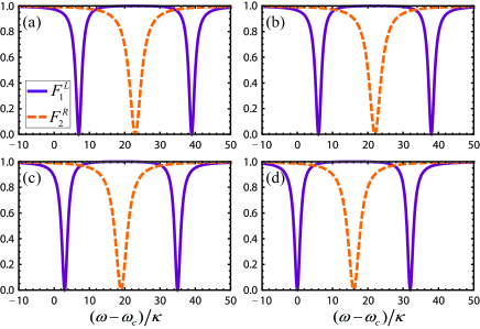
Figure 2: (color online) The spectrums of the scattering probabilities $F_{1}^{L}$ (purple solid lines) and $F_{2}^{R}$ (orange dashed lines) for driving frequency $\omega_{d}$: (a) $\omega_{d}/\kappa$ $=$ $4$, (b) $\omega_{d}/\kappa$ $=$ $6$, (c) $\omega_{d}/\kappa$ $=$ $12$, (d) $\omega_{d}/\kappa$ $=$ $18$. The other parameters are stated in the text.

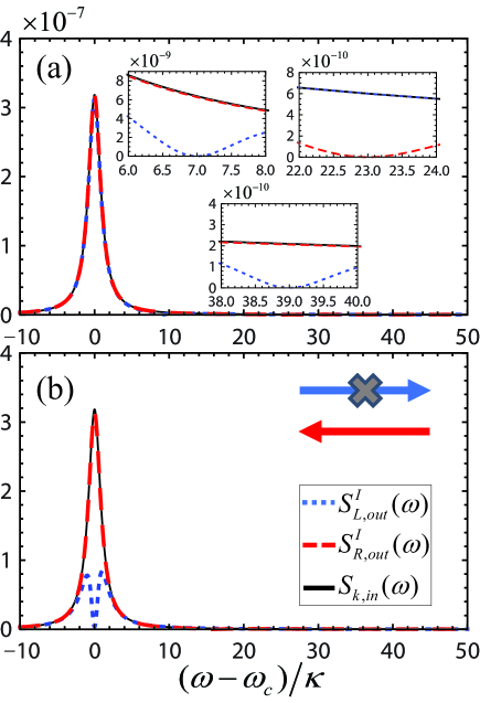
Figure 3: (color online) The spectrums of the output fields $S_{L,out}^{I}(\omega)$ (blue dotted lines), $S_{R,out}^{I}(\omega)$ (red dashed lines) and the input fields $S_{k,in}(\omega)$ (Black solid lines) for different driving frequency $\omega_{d}$: (a) $\omega_{d}/\kappa$ $=$ $4$, (b) $\omega_{d}/\kappa=18$. The other parameters are given in the text.

III Unidirectional isolation of the signal in the single-photon level

In this section, we numerically evaluate the scattering probabilities and the spectrums of the input-output fields to show the possibility of achieving the unidirectional isolation of the signal in the single-photon level. It should be pointed out that, we have plotted the spectrums of all the scattering probabilities $F_{1}^{L},\cdots,F_{6}^{L}$ and $F_{1}^{R},\cdots,F_{6}^{R}$, and found that in the range of the parameters we considered ($\varepsilon_{d}/\kappa$ $=$ $6$ $\times$ $10^{-5}$), the scattering probabilities have following order of magnitude: $F_{1}^{L}$ $\sim$ $1$, $F_{4}^{L}$ $\sim$ $10^{-9}$, $F_{2}^{L}$ $\sim$ $10^{-7}$, $F_{5}^{L}$ $\sim$ $10^{-15}$, $F_{3}^{L}$ $\sim$ $10^{-4}$, $F_{6}^{L}$ $\sim$ $10^{-13}$, and $F_{1}^{R}$ $\sim$ $10^{-7}$, $F_{4}^{R}$ $\sim$ $10^{-15}$, $F_{2}^{R}$ $\sim$ $1$, $F_{5}^{R}$ $\sim$ $10^{-22}$, $F_{3}^{R}$ $\sim$ $10^{-11}$, $F_{6}^{R}$ $\sim$ $10^{-19}$. In the single-photon level, the peak value of the spectrum of the input field $S_{k,in}(\omega)$ $\sim$ $10^{-7}$. Hence the spectrums of the output fields can be reduced to

$$S_{L,out}^{I}(\omega)=F_{1}^{L}S_{L,in}(\omega),S_{R,out}^{I}(\omega)=F_{2}^{R}S_{R,in}(\omega),$$ (27)

and we have assumed that the thermal phonon occupation number $n_{th}=0$.

As shown in Fig. 2(a), we plot the spectrums of the scattering probabilities $F_{1}^{L}$ and $F_{2}^{R}$ for different driving frequency $\omega_{d}$. We can see that the transmission of the left-going mode is simply that of a bare resonator, while the transmission of the right-going mode is modified by the presence of the MR, the effective optomechanical coupling $G_{L}$ will lead to a normal mode splitting 47 ; 48 in the strong coupling regime. With the presence of the weak coherent driving, the effective frequency of the mechanical mode becomes $\Delta_{m}=\omega_{m}-\omega_{d}/2.$ The above features will result in a unidirectional isolation between the left-going mode and right-going mode at three positions: at $\omega-\omega_{c}$ $=$ $\Delta_{m}$, we have $F_{1}^{L}$ $=$ $1$, $F_{2}^{R}$ $=$ $0$; at $\omega-\omega_{c}$ $=$ $\Delta_{m}$ $\pm$ $G_{L}$, we have $F_{1}^{L}$ $=$ $0$, $F_{2}^{R}$ $\lesssim$ $1$. When we increase $\omega_{d}$, the effective frequency $\Delta_{m}$ will decrease, and the curves will integrally move to the left.

To see the nonreciprocal transmission from the perspective of the spectrums of the output fields, we should also consider the spectrum of the input field. In Fig. 3, we plot the spectrum of the input field $S_{k,in}(\omega)$ as a comparison with the spectrums of the output fields. In Fig. 3(a), we use the same parameters as that in Fig. 2(a). It can be seen that, the non-reciprocity will indeed emerge at $\omega-\omega_{c}$ $=$ $\Delta_{m}$ and $\omega-\omega_{c}$ $=$ $\Delta_{m}\pm$ $G_{L}$. However, these points are all far away from the peak frequency of the input field, the values of $S_{k,in}(\omega)$ at these points are too small. The spectrums of the output fields $S_{L,out}^{I}(\omega)$, $S_{R,out}^{I}(\omega)$ and the input field $S_{k,in}(\omega)$ are almost coincide, and the nonreciprocity in this case can be ignored. By adjusting the driving frequency $\omega_{d}$, we can move the frequency where the non-reciprocity happens to the peak frequency of the single-photon. As shown in Fig. 3(b), we use the same parameters as that in Fig. 2(d). It can be seen that, at $\omega-\omega_{c}$ $=$ $0$, $S_{L,out}^{I}(\omega)$ $=0$, $S_{R,out}^{I}(\omega)$ $=$ $S_{k,in}(\omega)$. In this case, the nonreciprocity is very obvious. The signal can transmit from the right to the left, but can not transmit in the opposite direction. In this case, our system can act as a unidirectional isolator in the single-photon level.

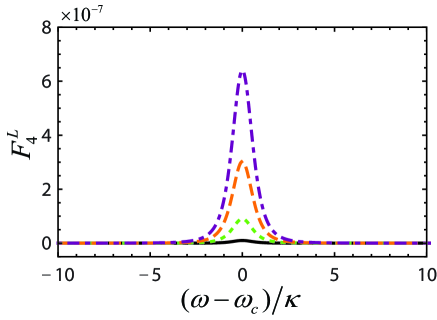
Figure 4: (color online) The spectrums of the scattering probabilities $F_{4}^{L}$ for different driving amplitude $\varepsilon_{d}$: (a) $\varepsilon_{d}/\kappa=1\times 10^{-4}$ (black solid line), (b) $\varepsilon_{d}/\kappa=3\times 10^{-4}$ (green dotted line), (c) $\varepsilon_{d}/\kappa=5.5\times 10^{-4}$ (orange dashed line), (d) $\varepsilon_{d}/\kappa=8\times 10^{-4}$ (purple dotdashed line), the other parameters are the same as in Fig. 2(d).

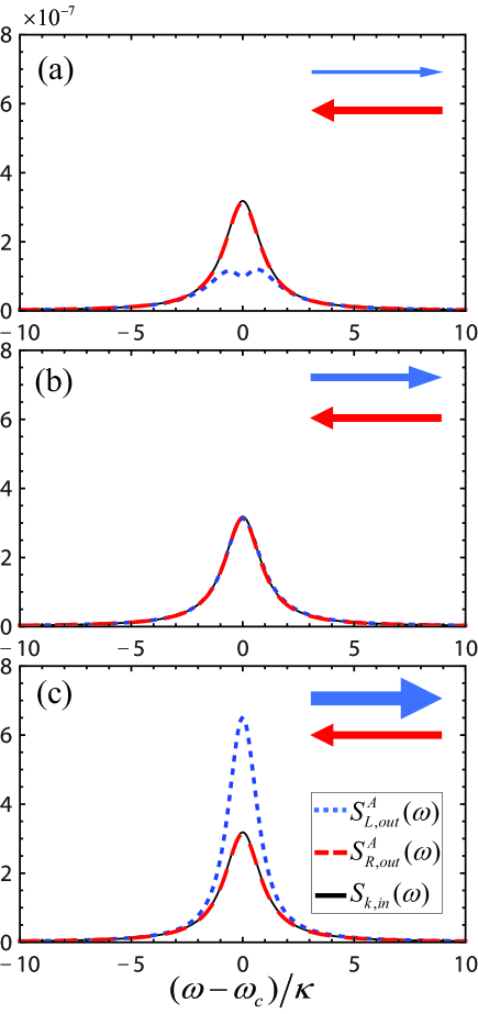
Figure 5: (color online) The spectrums of the output fields $S_{L,out}^{A}(\omega)$ (blue dotted lines), $S_{R,out}^{A}(\omega)$ (red dashed lines) and the input fields $S_{k,in}(\omega)$ (Black solid lines) for different driving amplitude $\varepsilon_{d}$ (a) $\varepsilon_{d}/\kappa=3\times 10^{-4}$, (b) $\varepsilon_{d}/\kappa=5.5\times 10^{-4}$, (c) $\varepsilon_{d}/\kappa=8\times 10^{-4}$. The other parameters are the same as that in Fig. 4.

IV Unidirectional amplification of the signal in the single-photon level

A previous work 40 has suggested that, such a weak coherent driving can induce a remarkable enhancement of the output fields. In this section, we will numerically evaluate the scattering probabilities and the spectrums of the input and output fields to show the possibility of achieving the unidirectional amplification of the signal in the single-photon level. Likewise, we have also plotted the spectrums of all the scattering probabilities $F_{1}^{L},\cdots,F_{6}^{L}$ and $F_{1}^{R},\cdots,F_{6}^{R}$. We find that, in the range of the parameters we considered ($1$ $\times$ $10^{-4}$ $\leq$ $\varepsilon_{d}/\kappa$ $\leq$ $8$ $\times$ $10^{-4}$), the scattering probabilities have the order of magnitude: $F_{1}^{L}$ $\sim$ $1$, $F_{4}^{L}$ $\sim$ $10^{-7}$, $F_{2}^{L}$ $\sim$ $10^{-7}$, $F_{5}^{L}$ $\sim$ $10^{-13}$, $F_{3}^{L}$ $\sim$ $10^{-4}$, $F_{6}^{L}$ $\sim$ $10^{-11}$, and $F_{1}^{R}$ $\sim$ $10^{-7}$, $F_{4}^{R}$ $\sim$ $10^{-13}$, $F_{2}^{R}$ $\sim$ $1$, $F_{5}^{R}$ $\sim$ $10^{-20}$, $F_{3}^{R}$ $\sim$ $10^{-11}$, $F_{6}^{R}$ $\sim$ $10^{-17}$. The peak value of the spectrum of the input field $S_{k,in}(\omega)$ $\sim$ $10^{-7}$. Hence the spectrums of the output fields can be reduced to

$$S_{L,out}^{A}(\omega) = F_{1}^{L}S_{L,in}(\omega)+F_{4}^{L},$$ (28)

$$S_{R,out}^{A}(\omega) = F_{2}^{R}S_{R,in}(\omega),$$ (29)

in which we have assumed that the thermal phonon occupation number $n_{th}=0$.

Since the amplitude of the weak coherent driving is very weak, we find that the scattering probabilities $F_{1}^{L}$ and $F_{2}^{R}$ are almost unchanged with the increase of $\varepsilon_{d}$. However, the weak coherent driving will induced a remarkable amplification on the scattering probabilities $F_{4}^{L}$, as shown in Fig. 4, with the increase of $\varepsilon_{d}$, at $\omega-\omega_{c}$ $=$ $0$, $F_{4}^{L}$ will gradually increase. This feature can be used to achieve the unidirectional amplification of the signal in the single-photon level.

From the perspective of the spectrums of the output fields, as shown in Fig. 5, with the increase of the driving amplitude $\varepsilon_{d}$, the value of the spectrum of the output field $S_{L,out}^{A}(\omega)$ at $\omega-\omega_{c}$ $=$ $0$ will increase, and the nonreciprocity will be weaken. When $\varepsilon_{d}$ reaches a certain threshold ($\varepsilon_{d}/\kappa$ $=$ $5.5\times 10^{-4}$), the nonreciprocity will almost disappear, i.e., $S_{L,out}^{A}(\omega)$ $\approx$ $S_{R,out}^{A}(\omega)$ $\approx$ $S_{k,in}(\omega)$. Furthermore, if we continue to increase the driving amplitude $\varepsilon_{d}$, the system will reveal a nonreciprocal amplification phenomenon as shown in Fig. 5(c), the signal transmitted from left to right can be amplified ($S_{R,out}^{A}(\omega)$ $>$ $S_{k,in}(\omega)$ at $\omega-\omega_{c}$ $=$ $0$), while the signal transmitted from right to left cannot be amplified ($S_{L,out}^{A}(\omega)$ $\approx$ $S_{k,in}(\omega)$ at $\omega-\omega_{c}$ $=$ $0$). In this case, our system can act as a unidirectional amplifier in the single-photon level.

V Discussion and Conclusion

Now we consider the effects of the mechanical thermal noise on the unidirectional isolator and amplifier. When the thermal phonon occupation number $n_{th}\neq 0$, the spectrums of the output fields become

$$S_{L,out}^{I}(\omega) = F_{1}^{L}S_{L,in}(\omega)+F_{3}^{L}n_{th},$$ (30)

$$S_{R,out}^{I}(\omega) = F_{2}^{R}S_{R,in}(\omega)+F_{3}^{R}n_{th},$$ (31)

$$S_{L,out}^{A}(\omega) = F_{1}^{L}S_{L,in}(\omega)+F_{4}^{L}+F_{3}^{L}n_{th},$$ (32)

$$S_{R,out}^{A}(\omega) = F_{2}^{R}S_{R,in}(\omega)+F_{3}^{R}n_{th}.$$ (33)

If the influence of the mechanical thermal noise can be neglected, we should ensure $F_{3}^{L}n_{th}$ $\ll$ $F_{1}^{L}S_{L,in}(\omega)$ and $F_{3}^{R}n_{th}$ $\ll$ $F_{2}^{R}S_{R,in}(\omega)$. From the above discussion, we have $F_{1}^{L}$, $F_{2}^{R}$ $\sim$ $1$, $F_{3}^{L}$ $\sim$ $10^{-4}$, $F_{3}^{R}$ $\sim$ $10^{-11}$, and $S_{k,in}(\omega)$ $\sim$ $10^{-7}$. Hence we should guarantee the thermal phonon occupation number $n_{th}$ $<$ $n_{thres}$ $\sim$ $10^{-4}$, i.e., the mechanical resonator should be cooled near its quantum ground state. However, if we choose a single-photon whose spectrum is narrower than the linewidth of the cavity, the threshold $n_{thres}$ can be improved. For example, if we choose $\Gamma=0.005\kappa,$ $S_{k,in}(\omega)$ can reach the order of magnitude $10^{-5}$, and $n_{thres}$ will be increased to $10^{-2}$. In addition, we can also increase the threshold $n_{thres}$ by improving the quality factor of the MR, when $Q_{m}$ $\sim$ $10^{8}$, $F_{3}^{L}$ will be reduced to $10^{-7}$, if $S_{k,in}(\omega)$ $\sim$ $10^{-7}$, $n_{thres}$ can reach the order of magnitude $10^{-1}$.

In summary, we have studied the single-photon nonreciprocal transmission in a cavity optomechanical system, in which the mechanical resonator is exciting by a weak coherent driving. We have shown that, if the input state is a single-photon state, it is insufficient to study the nonreciprocity only from the perspective of the transmission spectrums. Our scheme can be used as a unidirectional isolator or amplifier in the single-photon level. Our proposed model might eventually provide the basis for the applications on quantum information processing or quantum networks.

APPENDIX

We consider that the input field is made up of a sequence of pulses with exactly one photon per pulse, the operator of the input field $\hat{a}_{k,in}$ can be expressed as 49

$$\hat{a}_{k,in}=\int d\omega\xi(\omega)\hat{a}_{k,in}(\omega),$$ (A1)

where $\xi(\omega)$ is the spectral amplitude for describing the pulse shape of the single-photon. The operators of the input fields should satisfy the commutation relation $[\hat{a}_{k,in},\hat{a}_{k,in}^{{\dagger}}]$ $=$ $1$, $[\hat{a}_{k,in}(\Omega),\hat{a}_{k,in}^{{\dagger}}(\omega)]$ $=$ $\delta(\omega+\Omega)$, and $\int d\omega\left|\xi(\omega)\right|^{2}=1$. Generally, the spectrum of the single-photon $S_{k,in}(\omega)$ $\equiv$ $\left|\xi(\omega)\right|^{2}$ has two forms: the Gaussian lineshape, or the Lorentzian lineshape, which is in dependence on its luminescent source.

Now we can define a single-photon state as a superposition of a single excitation over many frequencies

$$\left|1_{\xi}\right\rangle=\hat{a}_{k,in}^{{\dagger}}\left|0\right\rangle=\int_{-\infty}^{+\infty}d\omega\xi^{\ast}(\omega)\hat{a}_{k,in}^{{\dagger}}(\omega)\left|0\right\rangle,$$ (A2)

so the correlation functions of the operators of the input fields can be obtained as

$$\left\langle\hat{a}_{k,in}^{{\dagger}}(\Omega)\hat{a}_{k,in}(\omega)\right\rangle =\left|\xi(\omega)\right|^{2}\delta(\omega+\Omega),$$ (A3)

$$\left\langle\hat{a}_{k,in}(\Omega)\hat{a}_{k,in}^{{\dagger}}(\omega)\right\rangle =[\left|\xi(\Omega)\right|^{2}+1]\delta(\omega+\Omega).$$ (A4)

References

• (1) L. Deák and T. Fülöp, Ann. Phys. (Amsterdam) 327, 1050 (2012).
• (2) J. Fujita, M. Levy, R. M. Osgood, Jr., L.Wilkens, and H.Dötsch, Appl. Phys. Lett. 76, 2158 (2000).
• (3) R. L. Espinola, T. Izuhara, M. C. Tsai, R. M. Osgood, Jr., and H. Dötsch, Opt. Lett. 29, 941 (2004).
• (4) F. D. M. Haldane and S. Raghu, Phys. Rev. Lett. 100, 013904 (2008).
• (5) Z.Wang, Y. Chong, J. D. Joannopoulos, and M. Soljačić, Nature (London) 461, 772 (2009).
• (6) L. Bi, J. Hu, P. Jiang, D. H. Kim, G. F. Dionne, L. C. Kimerling, and C. A. Ross, Nat. Photonics 5, 758 (2011).
• (7) Y. Shoji, M. Ito, Y. Shirato, and T. Mizumoto, Opt. Express 20, 18440 (2012).
• (8) X. Guo, C.-L. Zou, H. Jung, and H. X. Tang, Phys. Rev. Lett. 117, 123902 (2016).
• (9) F. Biancalana, J. Appl. Phys. 104, 093113 (2008).
• (10) C. Wang, C. Zhou, and Z. Li, Opt. Express 19, 26948 (2011).
• (11) K. Xia, M. Alamri, and M. S. Zubairy, Opt. Express 21, 25619 (2013).
• (12) E. J. Lenferink, G.Wei, and N. P. Stern, Opt. Express 22, 16099 (2014).
• (13) Z. F. Yu and S. H. Fan, Nat. Photonics 3, 91 (2009).
• (14) K. Fang, Z. Yu, and S. Fan, Nat. Photonics 6, 782 (2012).
• (15) E. Li, B. J. Eggleton, K. Fang, and S. Fan, Nat. Commun. 5, 3225 (2014).
• (16) C. R. Doerr, L. Chen, and D. Vermeulen, Opt. Express 22, 4493 (2014).
• (17) H. Lira, Z. F. Yu, S. H. Fan, and M. Lipson, Phys. Rev. Lett. 109, 033901 (2012).
• (18) M. C. Muñoz, A. Y. Petrov, L. O’Faolain, J. Li, T. F. Krauss, and M. Eich, Phys. Rev. Lett. 112, 053904 (2014).
• (19) Y. Yang, C. Galland, Y. Liu, K. Tan, R. Ding, Q. Li, K. Bergman, T. Baehr-Jones, and M. Hochberg, Opt. Express 22, 17409 (2014).
• (20) Q. Wang, F. Xu, Z. Y. Yu, X. S. Qian, X. K. Hu, Y. Q. Lu, and H. T. Wang, Opt. Express 18, 7340 (2010).
• (21) M. S. Kang, A. Butsch, and P. S. J. Russell, Nat. Photonics 5, 549 (2011).
• (22) C. Eüter, K. G. Makris, R. EI-Ganainy, D. N. Christodoulides, M. Segev, and D. Kip, Nat. Phys. 6, 192 (2010).
• (23) H. Ramezani, T. Kottos, R. El-Ganainy, and D. N. Christodoulides, Phys. Rev. A 82, 043803 (2010).
• (24) L. Feng, M. Ayache, J. Q. Huang, Y. L. Xu,M. H. Lu, Y. F. Chen, Y. Fainman, and A. Scherer, Science 333, 729 (2011).
• (25) J. H. Wu, M. Artoni, and G. C. La Rocca, Phys. Rev. Lett. 113, 123004 (2014).
• (26) D. W. Wang, H. T. Zhou, M. J. Guo, J. X. Zhang, J. Evers, and S. Y. Zhu, Phys. Rev. Lett. 110, 093901 (2013).
• (27) S. A. R. Horsley, J. H. Wu, M. Artoni, and G. C. La Rocca, Phys. Rev. Lett. 110, 223602 (2013).
• (28) S. Barzanjeh, M. Wulf, M. Peruzzo, M. Kalaee, P. B. Dieterle, O. Painter, and J. M. Fink, Nat. Commun. 8, 953 (2017).
• (29) S. Barzanjeh, M. Aquilina, and A. Xuereb, Phys. Rev. Lett. 120, 060601 (2018).
• (30) S. Manipatruni, J. T. Robinson, and M. Lipson, Phys. Rev. Lett. 102, 213903 (2009).
• (31) M. Hafezi and P. Rabl, Opt. Express 20, 7672 (2012).
• (32) X. W. Xu and Y. Li, Phys. Rev. A 91, 053854 (2015).
• (33) L. Tian and Z. Li, Phys. Rev. A 96, 013808 (2017).
• (34) D. Malz, L. D. Tóth, N. R. Bernier, A. K. Feofanov, T. J. Kippenberg, and A. Nunnenkamp, Phys. Rev. Lett. 120, 023601 (2018).
• (35) Y. Shen, M. Bradford, and J. T. Shen, Phys. Rev. Lett. 107, 173902 (2011).
• (36) E. Mascarenhas, D. Gerace, D. Valente, S. Montangero, A. Auffoves, and M. F. Santos, Europhys. Lett. 106, 54003 (2014).
• (37) D. Rugar and P. Grütter, Phys. Rev. Lett. 67, 699 (1991).
• (38) A. Szorkovszky, G. A. Brawley, A. C. Doherty, and W. P. Bowen, Phys. Rev. Lett. 110, 184301 (2013).
• (39) M. A. Lemonde, N. Didier, and A. A. Clerk, Nat. Commun. 7, 11338 (2016).
• (40) L. G. Si, H. Xiong, M. S. Zubairy, and Y. Wu, Phys. Rev. A 95, 033803 (2017).
• (41) G. S.Agarwal and S. Huang, Phys. Rev. A 85, 021801 (2012).
• (42) G. J. Milburn, Eur. Phys. J. Special Topics, 159, 113 (2008).
• (43) E. X. DeJesus and C. Kaufman, Phys. Rev. A 35, 5288 (1987).
• (44) D. Vitali, S. Gigan, A. Ferreira, H. R. Böhm, P. Tombesi, A. Guerreiro, V. Vedral, A. Zeilinger, and M. Aspelmeyer, Phys. Rev. Lett. 98, 030405 (2007).
• (45) R. Ghöbadi, A. R. Bahrampour, and C. Simon, Phys. Rev. A 84, 033846 (2011).
• (46) C. W. Gardiner and M. J. Collett, Phys. Rev. A 31, 3761 (1985).
• (47) J. M. Dobrindt, I. Wilson-Rae, and T. J. Kippenberg, Phys. Rev. Lett. 101, 263602 (2008).
• (48) S. Gröblacher, K. Hammerer, M. Vanner, and M. Aspelmeyer, Nature (London) 460, 724 (2009).
• (49) R. Loudon, The Quantum Theory of Light (Oxford University Press, Oxford, 2000).