Distributed Majorization-Minimization for Laplacian Regularized Problems

Abstract

We consider the problem of minimizing a block separable convex function (possibly nondifferentiable, and including constraints) plus Laplacian regularization, a problem that arises in applications including model fitting, regularizing stratified models, and multi-period portfolio optimization. We develop a distributed majorization-minimization method for this general problem, and derive a complete, self-contained, general, and simple proof of convergence. Our method is able to scale to very large problems, and we illustrate our approach on two applications, demonstrating its scalability and accuracy.

1 Introduction

Many applications, ranging from multi-period portfolio optimization [BBD⁺17] to joint covariance estimation [HPBL17], can be modeled as convex optimization problems with two objective terms, one that is block separable and the other a Laplacian regularization term [YGL16]. The block separable term can be nondifferentiable and may include constraints. The Laplacian regularization term is quadratic, and penalizes differences between individual variable components. These types of problems arise in several domains, including signal processing [PC17], machine learning [ST17], and statistical estimation or data fitting problems with an underlying graph prior [AZ06, MB11]. As such, there is a need for scalable algorithms to efficiently solve these problems.

In this paper we develop a distributed method for minimizing a block-separable convex objective with Laplacian regularization. Our method is iterative; in each iteration a convex problem is solved for each block, and the variables are then shared with each block’s neighbors in the graph associated with the Laplacian term. Our method is an instance of a standard and well known general method, majorization-minimization (MM) [Lan16], which recovers a wide variety of existing methods depending on the choice of majorization [SBP17]. In this paper, we derive a diagonal quadratic majorizer of the given Laplacian objective term, which has the benefit of separability. This separability allows for the minimization step in our MM algorithm to be carried out in parallel on a block-by-block basis. We develop a completely self-contained proof of convergence of our method, which relies on no further assumption than the existence of a solution. Finally, we apply our method to two separate applications, multi-period portfolio optimization and joint covariance estimation, demonstrating the scalable performance of our algorithm.

1.1 Related work

There has been extensive research on graph Laplacians and Laplacian regularization [GR01, WSZS07, RHL13], and on developing solvers specifically for use in optimization over graphs [HWD⁺17]. In addition, there has been much research done on the MM algorithm [AZ06, RHL13, Lan16, SBP17], including interpreting other well studied algorithms, such as the concave-convex procedure and the expectation-maximization algorithm [YR03, WL10] as special cases of MM. We are not aware of any previous work that applies the MM algorithm to Laplacian regularization.

There has also been much work on the two specific application examples that we consider. Multi-period portfolio optimization is studied in, for example, [AC00, SB09, BBD⁺17], although scalability remains an issue in these studies. Our second application example arises in signal processing, specifically the joint estimation of inverse covariance matrices, which has been studied and applied in many different contexts, such as cell signaling [FHT08, DWW14], statistical learning [BEGd08], and radar signal processing [SW17]. Again, scalability here is either not referenced or is still an ongoing issue in these fields.

1.2 Outline

In §2 we set up our notation, and describe the problem of Laplacian regularized minimization. In §3 we show how to construct a diagonal quadratic majorizer of a weighted Laplacian quadratic form. In §4 we describe our distributed MM algorithm, and give a complete and self-contained proof of convergence. Finally, in §5 we present numerical results for two applications which demonstrates the effectiveness of our method.

2 Laplacian regularized minimization

We consider the problem of minimizing a convex function plus Laplacian regularization,

$$\begin{array}[]{ll}\mbox{minimize}&F(x)=f(x)+\mathcal{L}(x),\end{array}$$ (1)

with variable $x\in{\mbox{\bf R}}^{n}$. Here $f:{\mbox{\bf R}}^{n}\to{\mbox{\bf R}}\cup\{\infty\}$ is a proper closed convex function [Roc70, BL00], and $\mathcal{L}:{\mbox{\bf R}}^{n}\rightarrow{\mbox{\bf R}}$ is the Laplacian regularizer (or Dirichlet energy [Eva10]) $\mathcal{L}(x)=(1/2)x^{T}Lx$, where $L$ is a weighted Laplacian matrix, i.e., $L=L^{T}$, $L_{ij}\leq 0$ for $i\neq j$, and $L\mathbf{1}=0$, where $\mathbf{1}$ is the vector with all entries one [GR01]. Associating with $\mathcal{L}$ the graph with vertices $1,\ldots,n$, edges indexed by pairs $(i,j)$ with $i<j$ and $L_{ij}\neq 0$, and (nonnegative) edge weights $w_{ij}=-L_{ij}$, the Laplacian regularizer can be expressed as

$$\mathcal{L}(z)=\sum_{(i,j)\in\mathcal{E}}w_{ij}(z_{i}-z_{j})^{2}.$$

We refer to the problem (1) as the Laplacian regularized minimization problem (LRMP). LRMPs are convex optimization problems, which can be solved by a variety of methods, depending on the specific form of $f$ [BV04, NW06]. We will let $F^{\star}$ denote the optimal value of the LRMP. Convex constraints can be incorporated into LRMP, by defining $f$ to take value $+\infty$ when the constraints are violated. Note in particular that we specifically do not assume that the function $f$ is finite, or differentiable (let alone with Lipschitz gradient), or even that its domain has affine dimension $n$. In this paper we will make only one additional analytical assumption about the LMRP (1): its sublevel sets are bounded. This assumption implies that the LRMP is solvable, i.e., there exists at least one optimal point $x^{\star}$, and therefore that its optimal value $F^{\star}$ is finite.

A point $x$ is optimal for the LRMP (1) if and only if there exists $g\in{\mbox{\bf R}}^{n}$ such that [Roc70, BL00]

$$g\in\partial f(x),\quad g+\nabla\mathcal{L}(x)=g+Lx=0,$$ (2)

where $\partial f(x)$ is the subdifferential of $f$ at $x$ [Roc70, Cla90]. For $g\in\partial f(x)$, we refer to

$$r=g+Lx$$

as the optimality residual for the LRMP (1). Our goal is to compute an $x$ (and $g\in\partial f(x)$) for which the residual $r$ is small.

We are interested in the case where $f$ is block separable. We partition the variable $x$ as $x=(x_{1},\ldots,x_{p})$, with $x_{i}\in{\mbox{\bf R}}^{n_{i}}$, $n_{1}+\cdots+n_{p}=n$, and assume $f$ has the form

$$f(x)=\sum_{i=1}^{p}f_{i}(x_{i}),$$

where $f_{i}:{\mbox{\bf R}}^{n}\to{\mbox{\bf R}}\cup\{\infty\}$ are closed convex proper functions.

The main contribution of this paper is a scalable and distributed method for solving LRMP in which each of the functions $f_{i}$ is handled separately. More specifically, we will see that each iteration of our algorithm requires the evaluation of a diagonally scaled proximal operator [PB14] associated with each block function $f_{i}$, which can be done in parallel.

3 Diagonal quadratic majorization of the Laplacian

Recall that a function $\hat{\mathcal{L}}:{\mbox{\bf R}}^{n}\times{\mbox{\bf R}}^{n}\rightarrow{\mbox{\bf R}}$ is a majorizer of $\mathcal{L}:{\mbox{\bf R}}^{n}\rightarrow{\mbox{\bf R}}$ if for all $x$ and $z$, $\hat{\mathcal{L}}(z;z)=\mathcal{L}(z)$, and $\hat{\mathcal{L}}(x;z)\geq\mathcal{L}(x)$ [Lan16, SBP17]. In other words, the difference $\hat{\mathcal{L}}(x,z)-\mathcal{L}(z)$ is nonnegative, and zero when $x=z$.

We now show how to construct a quadratic majorizer of the Laplacian regularizer $\mathcal{L}$. This construction is known [SBP17], but we give the proof for completeness. Suppose $\hat{L}=\hat{L}^{T}$ satisfies $\hat{L}\succeq L$, i.e., $\hat{L}-L$ is positive semidefinite. The function

$$\hat{\mathcal{L}}(x;z)=(1/2)z^{T}Lz+z^{T}L(x-z)+(1/2)(x-z)^{T}\hat{L}(x-z),$$ (3)

which is quadratic in $x$, is a majorizer of $\mathcal{L}$. To see this, we note that

$$\begin{array}[]{ll}\hat{\mathcal{L}}(x;z)-\mathcal{L}(x)&=(1/2)z^{T}Lz+z^{T}L(x-z)+(1/2)(x-z)^{T}\hat{L}(x-z)-(1/2)x^{T}Lx\\ &=(1/2)(x-z)^{T}(\hat{L}-L)(x-z),\end{array}$$

which is always nonnegative, and zero when $x=z$.

In fact, every quadratic majorizer of $\mathcal{L}$ arises from this construction, for some $\hat{L}\succeq L$. To see this we note that the difference $\hat{\mathcal{L}}(x;z)-\mathcal{L}(x)$ is a quadratic function of $x$ that is nonnegative and zero when $x=z$, so it must have the form $(1/2)(x-z)^{T}P(x-z)$ for some $P=P^{T}\succeq 0$. It follows that $\hat{\mathcal{L}}$ has the form (3), with $\hat{L}=P+L\succeq L$.

We now give a simple scheme for choosing $\hat{L}$ in the diagonal quadratic majorizer. Suppose $\hat{L}$ is diagonal,

$$\hat{L}=\mathop{\bf diag}(\alpha)=\mathop{\bf diag}(\alpha_{1},\ldots,\alpha_{n}),$$

where $\alpha\in{\mbox{\bf R}}^{n}$. A simple sufficient condition for $\hat{L}\succeq L$ is $\alpha_{i}\geq 2L_{ii}$, $i=1,\ldots,n$. This follows from standard results for Laplacians [Bol98], but it is simple to show directly. We note that for any $z\in{\mbox{\bf R}}^{n}$, we have

$$z^{T}(\hat{L}-L)z = \sum_{i=1}^{n}(\alpha_{i}-L_{ii})z_{i}^{2}+\sum_{i=1}^{n}\sum_{j\neq i}(-L_{ij})z_{i}z_{j}$$

$$\geq \sum_{i=1}^{n}L_{ii}z_{i}^{2}+\sum_{i=1}^{n}\sum_{j\neq i}L_{ij}|z_{i}||z_{j}|$$

$$= |z|^{T}L|z|\geq 0,$$

where the absolute value is elementwise. On the second line we use the inequalities $\alpha_{i}-L_{ii}\geq L_{ii}$ and for $j\neq i$, $-L_{ij}z_{i}z_{j}\geq L_{ij}|z_{i}||z_{j}|$, which follows since $L_{ij}\leq 0$.

In our algorithm described below, we will require that $\hat{L}\succ L$, i.e., $\hat{L}-L$ is positive definite. This can be accomplished by choosing

$$\alpha_{i}>2L_{ii},\quad i=1,\ldots,n.$$ (4)

There are many other methods for selecting $\alpha$, some of which have additional properties. For example, we can choose $\alpha=2\lambda_{\max}(L)\mathbf{1}$, where $\lambda_{\max}(L)$ denotes the maximum eigenvalue of $L$. With this choice we have $\hat{L}=2\lambda_{\max}(L)I$. This diagonal majorization has all diagonal entries equal, i.e., it is a multiple of the identity.

Another choice (that we will encounter later in §5.2) takes $\hat{L}$ to be a block diagonal matrix, conformal with the partition of $x$, with each block component a (possibly different) multiple of the identity,

$$\hat{L}=\mathop{\bf diag}(\alpha_{1}I_{n_{1}},\ldots,\alpha_{p}I_{n_{p}}),$$ (5)

where we can take

$$\alpha_{i}>\max_{j\in N_{i}}2L_{jj},\quad i=1,\ldots,p,$$

where $N_{i}$ is the index range for block $i$.

4 Distributed majorization-minimization algorithm

The majorization-minimization (MM) algorithm is an iterative algorithm that at each step minimizes a majorizer of the original function at the current iterate [SBP17]. Since $\hat{\mathcal{L}}$, as constructed in §3, using (4), majorizes $\mathcal{L}$, it follows that $\hat{F}=f+\hat{\mathcal{L}}$ majorizes $F=f+\mathcal{L}$. The MM algorithm for minimizing $F$ is then

$$x^{k+1}=\mathop{\rm argmin}_{x}\left(f(x)+\hat{\mathcal{L}}(x;x^{k})\right),$$ (6)

where the superscripts $k$ and $k+1$ denote the iteration counter. Note that since $\hat{L}$ is positive definite, $\hat{\mathcal{L}}$ is strictly convex in $x$, so the argmin is unique.

Stopping criterion.

The optimality condition for the update (6) is the existence of $g^{k+1}\in{\mbox{\bf R}}^{n}$ with

$$g^{k+1}\in\partial f(x^{k+1}),\quad g^{k+1}+\nabla\hat{\mathcal{L}}(x^{k+1};x^{k})=0.$$ (7)

From $\hat{\mathcal{L}}(x;z)-\mathcal{L}(x)=(1/2)(x-z)^{T}(\hat{L}-L)(x-z)$, we have

$$\nabla\hat{\mathcal{L}}(x^{k+1};x^{k})-\nabla{\mathcal{L}}(x^{k+1})=(\hat{L}-L)(x^{k+1}-x^{k}).$$

Substituting this into (7) we get

$$g^{k+1}+\nabla{\mathcal{L}}(x^{k+1})=(\hat{L}-L)(x^{k}-x^{k+1}).$$ (8)

Thus we see that

$$r^{k+1}=(\hat{L}-L)(x^{k}-x^{k+1})$$

is the optimality residual for $x^{k+1}$, i.e., the right-hand side of (2). We will use $\|r^{k+1}\|_{2}\leq\epsilon$, where $\epsilon>0$ is a tolerance, as our stopping criterion. This guarantees that on exit, $x^{k+1}$ satisfies the optimality condition (2) within $\epsilon$.

Absolute and relative tolerance.

When the algorithm is used to solve problems in which $x^{\star}$ or $L$ vary widely in size, the tolerance $\epsilon$ is typically chosen as a combination of an absolute error $\epsilon_{\mathrm{abs}}$ and a relative error $\epsilon_{\mathrm{rel}}$, for example,

$$\epsilon=\epsilon_{\mathrm{abs}}+\epsilon_{\mathrm{rel}}(\|{\hat{L}-L}\|_{F}+\|x\|_{2}),$$

where $\|\cdot\|_{F}$ denotes the Frobenius norm.

Distributed implementation.

The update (6) can be broken down into two steps. The first step requires multiplying by $L$, and in the other step, we carry out $p$ independent minimizations in parallel. We partition the Laplacian matrix $L$ into blocks $L_{ij},i,j=1,\ldots,p$, conformal with the partition $x=(x_{1},\ldots,x_{p})$. (In a few places above, we used $L_{ij}$ to denote the $i,j$ entry of $L$, whereas here we use it to denote the $i,j$ submatrix. This slight abuse of notation should not cause any confusion since the index ranges, and the dimensions, make it clear whether the entry, or submatrix, is meant.) We then observe that our majorizer (3) has the form

$$\hat{\mathcal{L}}(x;z)=\sum_{i=1}^{p}\hat{\mathcal{L}}_{i}(x_{i};z)+c,$$

where $c$ does not depend on $x$, and

$$\hat{\mathcal{L}}_{i}(x_{i};z)=(1/2)(x_{i}-z_{i})^{T}\hat{L}_{ii}(x_{i}-z_{i})+h_{i}^{T}x_{i},$$

where $z_{i}$ refers to the $i$th subvector of $z$, and $h_{i}$ is the $i$th subvector $Lz$,

$$h_{i}=L_{ii}z_{i}+\sum_{j\neq i}L_{ij}z_{j}.$$

It follows that

$$\hat{F}(x;x^{k})=\sum_{i=1}^{p}(f_{i}(x_{i})+\hat{\mathcal{L}}(x_{i};x_{i}^{k}))+c$$

is block separable.

• Algorithm 4.1  Distributed majorization-minimization.

  given Laplacian matrix $L$, and initial starting point $x^{0}$ in the feasible set of the problem,
  with $f(x^{0})<\infty$.
  Form majorizer matrix. Form diagonal $\hat{L}$ with $\hat{L}\succ L$ (using (4)).
  for $k=1,2,\ldots$
  	1. Compute linear term. Compute $h^{k}=Lx^{k}$ and residual $r^{k}=(\hat{L}-L)(x^{k-1}-x^{k})$.
  	2. Update in parallel. For $i=1,\ldots,p$, update each $x_{i}$ (in parallel) as
  	$x_{i}^{k+1}=\mathop{\rm argmin}_{x_{i}}\left(f_{i}(x_{i})+(1/2)(x_{i}-x_{i}^{k})^{T}\hat{L}_{ii}(x_{i}-x_{i}^{k})+(h_{i}^{k})^{T}x_{i}\right)$.
  	3. Test stopping criterion. Quit if $k\geq 2$ and $\|r^{k}\|_{2}\leq\epsilon$.

Step 1 couples the subvectors $x_{i}^{k}$; step 2 (the subproblem updates) is carried out in parallel for each $i$. We observe that the updates in step 2 are (diagonally scaled) proximal operator evaluations, i.e., they involve minimizing $f_{i}$ plus a norm squared term, with diagonal quadratic norm; see, e.g., [PB14]. Our algorithm can thus be considered as a distributed proximal-based method. We also mention that as the algorithm converges (discussed in detail below), $x_{i}^{k+1}-x_{i}^{k}\to 0$, which implies that the quadratic terms $(1/2)(x_{i}-x_{i}^{k})^{T}\hat{L}_{ii}(x_{i}-x_{i}^{k})$ and their gradients in the update asymptotically vanish; roughly speaking, they ‘go away’ as the algorithm converges. We will see below, however, that these quadratic terms are critical to convergence of the algorithm.

Warm start.

Our algorithm supports warm starting by choosing the initial point $x^{0}$ as an estimate of the solution, for example, the solution of a closely related problem. Warm starting can decrease the number of iterations required to converge [YW02, WB10]; we will see an example in §5.

4.1 Convergence

There are many general convergence results for MM methods, but all of them require varying additional assumptions about the objective function [Lan16, SBP17]. In this section we give a complete self-contained proof of convergence for our algorithm, that requires no additional assumptions. We will show that $F(x^{k})-F^{\star}\to 0$, as $k\to\infty$, and also that the stopping criterion eventually holds, i.e., $(\hat{L}-L)(x^{k}-x^{k+1})\to 0$.

We first observe a standard result that holds for all MM methods: The objective function is non-increasing. We have

$$F(x^{k+1})\leq\hat{F}(x^{k+1};x^{k})\leq\hat{F}(x^{k};x^{k})=F(x^{k}),$$

where the first inequality holds since $\hat{F}$ majorizes $F$, and the second since $x^{k+1}$ minimizes $\hat{F}(x;x^{k})$ over $x$. It follows that $F(x^{k})$ converges, and therefore $F(x^{k})-F(x^{k+1})\to 0$. It also follows that the iterates $x^{k}$ are bounded, since every iterate satisfies $F(x^{k})\leq F(x^{0})$, and we assume that the sublevel sets of $F$ are bounded.

Since $F$ is convex and $g^{k+1}+\nabla\mathcal{L}(x^{k+1})\in\partial F(x^{k+1})$, we have (from the definition of subgradient)

$$F(x^{k})\geq F(x^{k+1})+(g^{k+1}+\nabla\mathcal{L}(x^{k+1}))^{T}(x^{k}-x^{k+1}).$$

Using this and (8), we have

$$F(x^{k})-F(x^{k+1})\geq(x^{k}-x^{k+1})^{T}(\hat{L}-L)(x^{k}-x^{k+1}).$$

Since $F(x^{k})-F(x^{k+1})\to 0$ as $k\to\infty$, and $\hat{L}-L\succ 0$, we conclude that $x^{k+1}-x^{k}\to 0$ as $k\to\infty$. This implies that our stopping criterion will eventually hold.

Now we show that $F(x^{k})\to F^{\star}$. Let $x^{\star}$ be any optimal point. Then,

$$F^{\star}=F(x^{\star}) \geq F(x^{k+1})+((\hat{L}-L)x^{k}-\hat{L}x^{k+1}+Lx^{k+1})^{T}(x^{\star}-x^{k+1})$$

$$= F(x^{k+1})+(x^{k}-x^{k+1})^{T}(\hat{L}-L)(x^{\star}-x^{k+1}).$$

So we have

$$F(x^{k+1})-F^{\star}\leq-(x^{k}-x^{k+1})^{T}(\hat{L}-L)(x^{\star}-x^{k+1}).$$

Since $x^{k}-x^{k+1}\to 0$ as $k\to\infty$, and $x^{k+1}$ is bounded, the right-hand side converges to zero as $k\to\infty$, and so we conclude $F(x^{k+1})-F^{\star}\to 0$ as $k\to\infty$.

4.2 Variations

Arbitrary convex quadratic regularization.

While our interest is in the case when $\mathcal{L}$ is Laplacian regularization, the algorithm (and convergence proof) work when $\mathcal{L}$ is any convex quadratic, i.e., $L\succeq 0$, with the choice

$$\alpha_{i}>\sum_{j=1}^{n}|L_{ij}|,\quad i=1,\ldots,n,$$

replacing the condition (4). In fact, the condition (4) is a special case of this condition, for a Laplacian matrix.

Nonconvex $f$.

If the objective function in the LRMP is nonconvex, i.e., $f$ is nonconvex, then the method proposed in this paper can be extended as a heuristic for solving (1) for nonconvex $f$. It is emphasized that the most the algorithm can guarantee is a local optimum, rather than a global optimum [BV04].

5 Examples

In this section we describe two applications of our distributed method for solving LRMP, and report numerical results demonstrating its convergence and performance. We run all numerical examples on a 32-core AMD machine with 64 hyperthreads, using the Pathos multiprocessing package to carry out computations in parallel [McK17]. Our code is available online at https://github.com/cvxgrp/mm_dist_lapl.

5.1 Multi-period portfolio optimization

We consider the problem of multi-period trading with quadratic transaction costs; see [BMOW14, BBD⁺17] for more detail. We are to choose a portfolio of $n$ holdings $x_{t}\in{\mbox{\bf R}}^{n}$, for periods $t=1,\ldots,T$. We assume the $n$th holding is a riskless holding (i.e., cash). We choose the portfolios by solving the problem

$$\begin{array}[]{ll}\mbox{minimize}&\sum_{t=1}^{T}\left(f_{t}(x_{t})+(1/2)(x_{t}-x_{t-1})^{T}D_{t}(x_{t}-x_{t-1})\right),\end{array}$$ (9)

where $f_{t}$ is the convex objective function (and constraints) for the portfolio in period $t$, and the $D_{t}$’s are diagonal positive definite matrices. The initial portfolio $x_{0}$ is given and constant; $x_{1},\ldots,x_{T}$ are the variables. The quadratic term $(1/2)(x_{t}-x_{t-1})^{T}D_{t}(x_{t}-x_{t-1})$ is the transaction cost, i.e., the additional cost of trading to move from the previous portfolio $x_{t-1}$ to the current one $x_{t}$. We will assume that there is no transaction cost associated with cash, i.e., $(D_{t})_{nn}=0$.

The objective function $f_{t}$ typically includes negative expected return, one or more risk constraints or risk avoidance terms, shorting or borrow costs, and possibly other terms. It also can include constraints, such as the normalization $\mathbf{1}^{T}x_{t}=1$ (in which case $x_{t}$ are referred to as the portfolio weights), limits on the holdings or the leverage of the portfolio, or a specified final portfolio; see [BMOW14, BBD⁺17] for more detail.

We can express the transaction cost as Laplacian regularization on $x=(x_{1},\ldots,x_{T})\in{\mbox{\bf R}}^{Tn}$, plus a quadratic term involving $x_{1}$,

$$\sum_{t=1}^{T}(1/2)(x_{t}-x_{t-1})^{T}D_{t}(x_{t}-x_{t-1})$$

$$= (1/2)x^{T}Lx+(1/2)x_{1}^{T}D_{1}x_{1}-(D_{1}x_{0})^{T}x_{1}+(1/2)x_{0}^{T}D_{1}x_{0}.$$

(Recall that the initial portfolio $x_{0}$ is given.) The Laplacian matrix $L$ has block-tridiagonal form given by

$$L=\begin{bmatrix}D_{2}&-D_{2}&0&\ldots&0&0&0\\ -D_{2}&D_{2}+D_{3}&-D_{3}&\ldots&0&0&0\\ 0&-D_{3}&D_{3}+D_{4}&\ldots&0&0&0\\ \vdots&\vdots&\vdots&\ddots&\vdots&\vdots&\vdots\\ 0&0&0&\ldots&D_{T-2}+D_{T-1}&-D_{T-1}&0\\ 0&0&0&\ldots&-D_{T-1}&D_{T-1}+D_{T}&-D_{T}\\ 0&0&0&\ldots&0&-D_{T}&D_{T}\end{bmatrix}.$$

If we assume that the initial portfolio is cash, i.e., $x_{0}$ is zero except in the last component, then two of the three extra terms, $(D_{1}x_{0})^{T}x_{1}$ and $(1/2)x_{0}^{T}D_{1}x_{0}$, both vanish. If we lump the extra terms that depend on $x_{1}$ into $f_{1}$, the multi-period portfolio optimization problem (9) has the LRMP form, with $p=T$ and $n_{i}=n$. The total number of (scalar) variables is $Tn$. The graph associated with the Laplacian is the simple chain graph; roughly speaking, each portfolio $x_{t}$ is linked to its predecessor $x_{t-1}$ and its successor $x_{t+1}$ by the transaction cost.

We can give a simple interpretation for the subproblem update in our method. The quadratic term of the subproblem update (which asymptotically goes away as we approach convergence) adds diagonal risk; the linear term $h_{t}$ contributes an expected return to each asset. These additional risk and return terms come from both the preceding and the successor portfolios; they ‘encourage’ the portfolios to move towards each other from one time period to the next, so as to reduce transaction cost. Each subproblem update minimizes negative risk-adjusted return, with the given return vector modified to encourage less trading.

5.1.1 Problem instance

We consider a problem with $n=1000$ assets and $T=30$ periods, so the total number of (scalar) variables is $30000$. The objective functions $f_{t}$ include a negative expected return, a quadratic risk given by a factor (diagonal plus low rank) model with 50 factors [CR83, BBD⁺17], and a linear shorting cost. We additionally impose the normalization constraint $\mathbf{1}^{T}x_{t}=1$, so the portfolios $x_{t}$ represent weights. The objective functions $f_{t}$ have the form

$$f_{t}(x)=-\mu_{t}^{T}x+\gamma x^{T}\Sigma_{t}x+s_{t}^{T}(x)_{-},\quad t=1,\ldots,T-1.$$ (10)

Here, $\gamma>0$ is the risk aversion parameter, $\mu_{t}$ is the expected return, $\Sigma_{t}$ is the return covariance, and $s_{t}$ is the (positive) shorting cost coefficient vector. The covariance matrices $\Sigma_{t}$ are diagonal plus a rank 50 (factor) term, with zero entries in the last row and column (which correspond to the cash asset). We choose all these coefficients and the diagonal transaction cost matrices $D_{t}$ randomly, but with realistic values. In our problem instance, we choose all of these parameters independent of $t$, i.e., constant.

We take $f_{T}$ to be the indicator function for the constraint $x=e_{n}$ (i.e., $f_{T}(x)=0$ if $x=e_{n}$, and $\infty$ otherwise), and the initial portfolio is all cash, $x_{0}=e_{n}$. So in our multi-period portfolio optimization problem we are planning a sequence of portfolios that begin and end in cash.

We can see the interpretation of the subproblem updates in §5.1 by looking at the subproblem objective functions. Assuming we choose the diagonal elements of $\hat{L}$ to be $3L_{ii}$, we can rewrite the subproblem objective function (at time periods $t=2,\ldots,T-1$ and iteration $k$) as

$$\begin{array}[]{ll}x_{t}^{T}(\gamma\Sigma_{t}+(3/2)(D_{t}+D_{t+1}))x_{t}-(\mu_{t}+D_{t}(2x_{t}^{k}-x_{t-1}^{k})+D_{t+1}(2x_{t}^{k}-x_{t+1}^{k}))^{T}x_{t}+c,\end{array}$$

where $c$ is some constant that does not depend on $x_{t}$. We see that a diagonal risk term is added, and the mean return $\mu_{t}$ is offset by terms that depend on the past, current, and future portfolios $x_{t-1}^{k}$, $x_{t}^{k}$, and $x_{t+1}^{k}$.

5.1.2 Numerical results

We first solve the problem instance using CVXPY [DB16] and solver OSQP [SBG⁺17], which is single-thread. The solve time for this baseline method was 120 minutes.

We then solved the problem instance using our method. We initialized all portfolios as $e_{n}$, i.e., all cash, and use stopping criterion tolerance $\epsilon=10^{-6}$. Our algorithm took 8 iterations and 19 seconds to converge, and produced a solution that agreed very closely with the CVXPY/OSQP solution. Figure 1 shows a plot of the residual norm $\|r^{k}\|_{2}$ versus iteration $k$. Ths plot shows nearly linear convergence, with a reduction in residual norm by around a factor of $5$ each iteration.

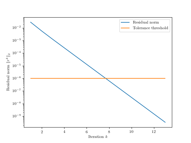
Figure 1: Residual norm versus iteration for multi-period portfolio optimization problem.

5.2 Laplacian regularized estimation

We consider estimation of parameters in a statistical model. We have a graph, with some data associated with each node; the goal is to fit a model to the data at each node, with Laplacian regularization used to make neighboring models similar.

The model parameter at node $i$ is $\theta_{i}\in{\mbox{\bf R}}^{n_{i}}$. The vector of all node parameters is $\theta=(\theta_{1},\ldots,\theta_{p})\in{\mbox{\bf R}}^{n}$, with $n=n_{1}+\cdots+n_{p}$. We choose $\theta$ by minimizing a local loss function and regularizer at each node, plus Laplacian regularization:

$$\begin{array}[]{ll}\mbox{minimize}&\sum_{i=1}^{p}f_{i}(\theta_{i})+\mathcal{L}(\theta),\end{array}$$

where $f_{i}(\theta_{i})=\ell_{i}(\theta_{i})+r_{i}(\theta_{i})$, where $\ell_{i}:{\mbox{\bf R}}^{n_{i}}\to{\mbox{\bf R}}$ is the loss function (for example, the negative log-likelihood of $\theta_{i}$) for the data at node $i$, and $r_{i}:{\mbox{\bf R}}^{n_{i}}\to{\mbox{\bf R}}$ is a regularizer on the parameter $\theta_{i}$. Without the Laplacian term, the problem is separable, and corresponds to fitting each parameter separately by minimizing the local loss plus regularizer. The Laplacian term is an additional regularizer that encourages various entries in the parameter vectors to be close to each other.

Laplacian regularized covariance estimation.

We now focus on a more specific case of this general problem, Laplacian regularized covariance estimation. At each node, we have some number of samples from a zero-mean Gaussian distribution on ${\mbox{\bf R}}^{d}$, with covariance matrix $\Sigma_{i}$, assumed positive definite. We will estimate the natural parameters (as an exponential family), the inverse covariance matrices $\theta_{i}=\Sigma_{i}^{-1}$. So here we take the node parameters $\theta_{i}$ to be symmetric positive definite $d\times d$ matrices, with $n_{i}=d(d+1)/2$. (In the discussion of the general case above, $\theta_{i}$ is a vector in ${\mbox{\bf R}}^{n_{i}}$; in the rest of this section, $\theta_{i}$ will denote a symmetric $d\times d$ martix.)

The data samples at node $i$ have empirical covariance $S_{i}$ (which is not positive definite if there are fewer than $d$ samples). The negative log-likelihood for node $i$ is (up to a constant and a positive scale factor)

$$\ell_{i}(\theta_{i})=\mathop{\bf Tr}(S_{i}\theta_{i})-\log\det\theta_{i}.$$

We use trace regularization on the parameter,

$$r_{i}(\theta_{i})=\kappa\mathop{\bf Tr}(\theta_{i}),$$

where $\kappa>0$ is the local regularization hyperparameter. We note that we can minimize $f_{i}(\theta_{i})=\ell_{i}(\theta_{i})+r_{i}(\theta_{i})$ analytically; the minimizer is

$$\theta_{i}=(S_{i}+\kappa I)^{-1}.$$

(See, e.g., [BEGd08].)

The Laplacian regularization is used to encourage neighboring inverse covariance matrices in the given graph to be near each other. It has the specific form

$$\mathcal{L}(\theta_{1},\ldots,\theta_{p})=\lambda\sum_{(i,j)\in\mathcal{E}}\|\theta_{i}-\theta_{j}\|_{F}^{2}=\mathop{\bf Tr}(\theta^{T}L\theta),$$

where the norm is the Frobenius norm, $L$ is the associated weighted Laplacian matrix for the graph with vertices $1,\ldots,p$ and edges $\mathcal{E}$, and $\lambda\geq 0$ is a hyperparameter that controls the amount of Laplacian regularization. When $\lambda=0$, the estimation problem is separable, with analytical solution

$$\theta_{i}=(S_{i}+\kappa I)^{-1},\quad i=1,\ldots,p.$$

For $\lambda\to\infty$, assuming the graph is connected, the estimation problem reduces to finding a single covariance matrix for all the data, with analytical solution

$$\theta_{i}=(S+p\kappa I)^{-1},\quad i=1,\ldots,p,$$

where $S=\sum_{j=1}^{p}S_{j}$ is the empirical covariance of all the data together.

We choose the majorizer to be block diagonal with each block a multiple of the identity, as in (5). The update at each node in our algorithm can be expressed as minimizing over $\theta_{i}$ the function

$$\mathop{\bf Tr}((S_{i}+H_{i}^{k})\theta_{i})-\log\det\theta_{i}+\kappa\mathop{\bf Tr}(\theta_{i})+(\alpha_{i}/2)\|\theta_{i}-\theta_{i}^{k}\|_{F}^{2},$$

where

$$H^{k}=L\theta^{k}.$$

This minimization can be carried out analytically. By taking the gradient of the subproblem objective function with respect to $\theta_{i}$ and equating to zero, we see that

$$S_{i}+H_{i}^{k}-\theta_{i}^{-1}+\kappa I+\alpha_{i}(\theta_{i}-\theta_{i}^{k})=0,$$

or

$$\theta_{i}^{-1}-\alpha_{i}\theta_{i}=S_{i}+H_{i}^{k}+\kappa I-\alpha_{i}\theta_{i}^{k}.$$

This implies that $\theta_{i}$ and $S_{i}+H_{i}^{k}+\kappa I-\alpha_{i}\theta_{i}^{k}$ share the same eigenvectors [WT09, DWW14, HPBL17]. Let $Q_{i}\Lambda_{i}Q_{i}^{T}$ be the eigenvector decomposion of $S_{i}+H_{i}^{k}+\kappa I-\alpha_{i}\theta_{i}^{k}$. We find that the eigenvalues of $\theta_{i},v_{ij},j=1,\ldots,n$, are

$$v_{ij}=(1/2\alpha_{i})\left(-(\Lambda_{i})_{jj}+\sqrt{(\Lambda_{i})_{jj}^{2}+4\alpha_{i}}\right).$$

We have $\theta_{i}^{k+1}=Q_{i}V_{i}Q_{i}^{T}$, where $V_{i}=\mathop{\bf diag}(v_{i1},\ldots,v_{in})$. The computational cost per iteration is primarily in computing the eigenvector decomposition of $S_{i}+H_{i}^{k}+\kappa I-\alpha_{i}\theta_{i}^{k}$, which has order $d^{3}$.

5.2.1 Problem instance

The graph is a $15\times 15$ grid, with 420 edges, so $p=225$. The dimension of the data is $d=30$, so each $\theta_{i}$ is a symmetric $30\times 30$ matrix. The total number of (scalar) variables in our problem instance is $225\times 30(30+1)/2=104625$.

We generate the data for each node as follows. First, we choose the four corner covariance matrices randomly. The other 221 nodes are given covariance matrices using bilinear interpolation from the corner covariance matrices. We then generate 20 independent samples of data from each of the node distributions. (The samples are in ${\mbox{\bf R}}^{30}$, so the empirical covariance matrices are singular.) In our problem instance we used hyperparameter values $\lambda=.053$ and $\kappa=0.08$, which were chosen to give good estimation performance.

5.2.2 Numerical results

The problem instance is too large to reliably solve using CVXPY and the solver SCS [OCPB16], which stops after two hours with the status message that the computed solution may be inaccurate.

We solved the problem using our distributed method, with absolute tolerance $\epsilon_{\mathrm{abs}}=10^{-5}$ and relative tolerance $\epsilon_{\mathrm{rel}}=10^{-3}$. The method took 54 iterations and 13 seconds to converge. Figure 2 is a plot of the residual norm $\|r^{k}\|_{F}$ versus iteration $k$.

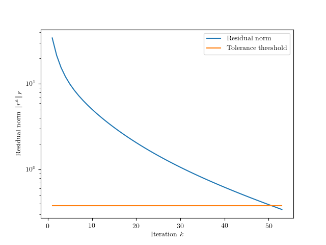
Figure 2: Residual norm vs. iteration for Laplacian regularized covariance estimation problem.

Regularization path via warm-start.

To illustrate the advantage of warm-starting our algorithm, we compute the entire regularization path, i.e., the solutions of the problem for 100 values of $\lambda$, spaced logarithmically between $10^{-5}$ and $10^{4}$.

Computing these 100 estimates by running the algorithm for each value of $\lambda$ sequentially, without warm-start, requires 26000 total iterations (an average of 260 iterations per choice of $\lambda$) and 81 minutes. Computing these 100 estimates by running the algorithm using warm-start, starting from $\lambda=10^{-5}$, requires only 2000 total iterations (an average of 20 iterations per choice of $\lambda$) and 7.1 minutes. For the specific instance solved above, the algorithm converges in only 2.5 seconds and 10 iterations using warm-start, compared to 13 seconds and 54 iterations using cold-start.

While the point of this example is the algorithm that computes the estimates, we also explore the performance of the method. For each of the 100 values of $\lambda$ we compute the root-mean-square error between our estimate of the inverse covariance and the true inverse covariance, which we know, since we generated them. Figure 3 shows a plot of the root-mean-square error of our estimate versus the value of $\lambda$. This plot shows that the method works, i.e., produces better estimates of the inverse covariance matrices than handling them separately (small $\lambda$) or fitting one inverse covariance matrix for all nodes (large $\lambda$).

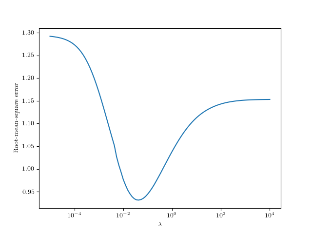
Figure 3: Root-mean-square error of the optimal estimates vs. $\lambda$.

References

- [AC00] R. Almgren and N. Chriss. Optimal execution of portfolio transactions. Journal of Risk, pages 5–39, 2000.
- [AZ06] R. K. Ando and T. Zhang. Learning on graph with Laplacian regularization. Conference on Neural Information Processing Systems, 2006.
- [BBD+17] S. Boyd, E. Busseti, S. Diamond, R. N. Kahn, K. Koh, P. Nystrup, and J. Speth. Multi-period trading via convex optimization. Foundations and Trends in Optimization, 3(1):1–76, April 2017.
- [BEGd08] O. Banerjee, L. El Ghaoui, and A. d’Aspremont. Model selection through sparse maximum likelihood estimation for multivariate Gaussian or binary data. Journal of Machine Learning Research, 9:485–516, 2008.
- [BL00] J. M. Borwein and A. S. Lewis. Convex Analysis and Nonlinear Optimization, Theory and Examples. Springer, 2000.
- [BMOW14] S. Boyd, M. T. Mueller, B. O’Donoghue, and Y. Wang. Performance bounds and suboptimal policies for multi-period investment. Foundations and Trends in Optimization, 1(1):1–72, January 2014.
- [Bol98] B. Bollobás. Modern Graph Theory. Graduate Texts in Mathematics. Springer, Heidelberg, 1998.
- [BV04] S. Boyd and L. Vandenberghe. Convex Optimization. Cambridge University Press, 2004.
- [Cla90] F. H. Clarke. Optimization and Nonsmooth Analysis. Society for Industrial and Applied Mathematics, 1990.
- [CR83] G. Chamberlain and M. Rothschild. Arbitrage, factor structure, and mean-variance analysis on large asset markets. Econometrica, 51(5):1281–1304, 1983.
- [DB16] S. Diamond and S. Boyd. CVXPY: A Python-embedded modeling language for convex optimization. Journal of Machine Learning Research, 17(83):1–5, 2016.
- [DWW14] P. Danaher, P. Wang, and D. M. Witten. The joint graphical lasso for inverse covariance estimation across multiple classes. Journal of the Royal Statistical Society, 76(2):373–397, 2014.
- [Eva10] L. C. Evans. Partial differential equations. American Mathematical Society, Providence, R.I., 2010.
- [FHT08] J. Friedman, T. Hastie, and R. Tibshirani. Sparse inverse covariance estimation with the graphical lasso. Biostatistics, 9(3):432–441, 08 2008.
- [GR01] C. Godsil and G. Royle. The Laplacian of a Graph. Springer, 2001.
- [HPBL17] D. Hallac, Y. Park, S. Boyd, and J. Leskovec. Network inference via the time-varying graphical lasso. Proceedings of the 23rd ACM SIGKDD International Conference on Knowledge Discovery and Data Mining, pages 205–213, 2017.
- [HWD+17] D. Hallac, C. Wong, S. Diamond, R. Sosic, S. Boyd, and J. Leskovec. SnapVX: A network-based convex optimization solver. Journal of Machine Learning Research, 18, 2017.
- [Lan16] K. Lange. MM Optimization Algorithms. Society for Industrial and Applied Mathematics, Philadelphia, PA, 2016.
- [MB11] S. Melacci and M. Belkin. Laplacian support vector machines trained in the primal. Journal of Machine Learning Research, 12:1149–1184, July 2011.
- [McK17] M. McKerns. Pathos multiprocessing, July 2017. Available at https://pypi.python.org/pypi/pathos.
- [NW06] J. Nocedal and S. J. Wright. Numerical Optimization. Springer, 2006.
- [OCPB16] B. O’Donoghue, E. Chu, N. Parikh, and S. Boyd. Conic optimization via operator splitting and homogeneous self-dual embedding. Journal of Optimization Theory and Applications, 169(3):1042–1068, June 2016.
- [PB14] N. Parikh and S. Boyd. Proximal algorithms. Foundations and Trends in Optimization, 1(3):127–239, January 2014.
- [PC17] J. Pang and G. Cheung. Graph laplacian regularization for image denoising: Analysis in the continuous domain. IEEE Transactions on Image Processing, 26(4):1770–1785, April 2017.
- [RHL13] M. Razaviyayn, M. Hong, and Z.Q. Luo. A unified convergence analysis of block successive minimization methods for nonsmooth optimization. SIAM Journal on Optimization, 23(2):1126–1153, 2013.
- [Roc70] R. T. Rockafellar. Convex Analysis. Princeton Mathematical Series. Princeton University Press, 1970.
- [SB09] Joëlle Skaf and Stephen Boyd. Multi-period portfolio optimization with constraints and transaction costs, 2009.
- [SBG+17] B. Stellato, G. Banjac, P. Goulart, A. Bemporad, and S. Boyd. OSQP: An operator splitting solver for quadratic programs. ArXiv e-prints, November 2017.
- [SBP17] Y. Sun, P. Babu, and D. Palomar. Majorization-minimization algorithms in signal processing, communications, and machine learning. IEEE Transactions in Signal Processing, 65(3):794–816, 2017.
- [ST17] D. Slepcev and M. Thorpe. Analysis of p-laplacian regularization in semi-supervised learning. ArXiV preprint, October 2017.
- [SW17] I. Soloveychik and A. Wiesel. Joint estimation of inverse covariance matrices lying in an unknown subspace. IEEE Transactions on Signal Processing, 65(9):2379–2388, 2017.
- [WB10] Y. Wang and S. Boyd. Fast model predictive control using online optimization. IEEE Transactions on Control Systems Technology, 18(3):267–278, March 2010.
- [WL10] T. T. Wu and K. Lange. The MM alternative to EM. Statistical Science, 25(4):492–505, 11 2010.
- [WSZS07] K. Q. Weinberger, F. Sha, Q. Zhu, and L. K. Saul. Graph Laplacian regularization for large-scale semidefinite programming. In Advances in Neural Information Processing Systems 19, pages 1489–1496. MIT Press, 2007.
- [WT09] D. M. Witten and R. Tibshirani. Covariance-regularized regression and classification for high dimensional problems. Journal of the Royal Statistical Society, 71(3):615–636, 2009.
- [YGL16] M. Yin, J. Gao, and Z. Lin. Laplacian regularized low-rank representation and its applications. IEEE Transactions on Pattern Analysis and Machine Intelligence, 38(3):504–517, March 2016.
- [YR03] A. L. Yuille and A. Rangarajan. The concave-convex procedure. Neural Computing, 15(4):915–936, April 2003.
- [YW02] E. Yildirim and S. Wright. Warm-start strategies in interior-point methods for linear programming. SIAM Journal on Optimization, 12(3):782–810, 2002.