Smoothed Online Convex Optimization in High Dimensions  
via Online Balanced Descent

Abstract

We study smoothed online convex optimization, a version of online convex optimization where the learner incurs a penalty for changing her actions between rounds. Given a $\Omega(\sqrt{d})$ lower bound on the competitive ratio of any online algorithm, where $d$ is the dimension of the action space, we ask under what conditions this bound can be beaten. We introduce a novel algorithmic framework for this problem, Online Balanced Descent (OBD), which works by iteratively projecting the previous point onto a carefully chosen level set of the current cost function so as to balance the switching costs and hitting costs. We demonstrate the generality of the OBD framework by showing how, with different choices of “balance,” OBD can improve upon state-of-the-art performance guarantees for both competitive ratio and regret; in particular, OBD is the first algorithm to achieve a dimension-free competitive ratio, $3+O(1/\alpha)$, for locally polyhedral costs, where $\alpha$ measures the “steepness” of the costs. We also prove bounds on the dynamic regret of OBD when the balance is performed in the dual space that are dimension-free and imply that OBD has sublinear static regret.

1 Introduction

In this paper we develop a new algorithmic framework, Online Balanced Descent (OBD), for online convex optimization problems with switching costs, a class of problems termed smoothed online convex optimization (SOCO). Specifically, we consider a setting where a learner plays a series of rounds $1,2,\ldots,T$. In each round, the learner observes a convex cost function $f_{t}$, picks a point $x_{t}$ from a convex set $\mathcal{X}$, and then incurs a hitting cost $f_{t}(x_{t})$. Additionally, she incurs a switching cost for changing her actions between successive rounds, $\|x_{t}-x_{t-1}\|$, where $\|\cdot\|$ is a norm.

This setting generalizes classical Online Convex Optimization (OCO), and has received considerable attention in recent years as a result of the recognition that switching costs play a crucial role in many learning, algorithms, control, and networking problems. In particular, many applications have, in reality, some cost associated with a change of action that motivates the learner to adopt “smooth” sequences of actions. For example, switching costs have received considerable attention in the $k$-armed bandit setting (Agrawal et al., 1990; Guha and Munagala, 2009; Koren et al., 2017) and the core of the Metrical Task Systems (MTS) literature is determining how to manage switching costs, e.g., the $k$-server problem (Borodin et al., 1992; Borodin and El-Yaniv, 2005).

Outside of learning, SOCO has received considerable attention in the networking and control communities. In these problems there is typically a measurable cost to changing an action. For example, one of the initial applications where SOCO was adopted is the dynamic management of service capacity in data centers (Lin et al., 2011; Lu et al., 2013), where the wear-and-tear costs of switching servers into and out of deep power-saving states is considerable. Other applications where SOCO has seen real-world deployment are the dynamic management of routing between data centers (Lin et al., 2012; Wang et al., 2014), management of electrical vehicle charging (Kim and Giannakis, 2014), video streaming (Joseph and de Veciana, 2012), speech animation (Kim et al., 2015), multi-timescale control (Goel et al., 2017), power generation planning (Badiei et al., 2015), and the thermal management of System-on-Chip (SoC) circuits (Zanini et al., 2009, 2010).

High-dimensional SOCO.

An important aspect of nearly all the problems mentioned above is that they are high-dimensional, i.e., the dimension $d$ of the action space is large. For example, in the case of dynamic management of data centers the dimension grows with the heterogeneity of the storage and compute nodes in the cluster, as well as the heterogeneity of the incoming workloads. However, the design of algorithms for high-dimensional SOCO problems has proven challenging, with fundamental lower bounds blocking progress.

Initial results on SOCO focused on finding competitive algorithms in the low-dimensional settings. Specifically, Lin et al. (2011) introduced the problem in the one-dimensional case and gave a 3-competitive algorithm. A few years later, Bansal et al. (2015) gave a 2-competitive algorithm, still for the one-dimensional case. Following these papers, Antoniadis et al. (2016) claimed that SOCO is equivalent to the classical problem of Convex Body Chasing Friedman and Linial (1993), in the sense that a competitive algorithm for one problem implies the existence of a competitive problem for the other. Using this connection, they claimed to show the existence of a constant competitive algorithm for two-dimensional SOCO. However, their analysis turned out to have a bug and their claims have been retracted (Pruhs, 2018). However, the connection to Convex Body Chasing does highlight a fundamental limitation. In particular, it is not possible to design a competitive algorithm for high-dimensional SOCO without making restrictions on the cost functions considered since, as we observe in Section 2, for general convex cost functions and $\ell_{2}$ switching costs, the competitive ratio of any algorithm is $\Omega(\sqrt{d})$.

The importance of high-dimensional SOCO problems in practical applications has motivated the “beyond worst-case” analysis for SOCO as a way of overcoming the challenge of designing constant competitive algorithms in high dimensions. To this end, Lin et al. (2012); Andrew et al. (2013); Chen et al. (2015); Badiei et al. (2015); Chen et al. (2016) all explored the value of predictions in SOCO, highlighting that it is possible to provide constant-competitive algorithms for high-dimensional SOCO problems using algorithms that have predictions of future cost functions, e.g., Lin et al. (2012) gave an algorithm based on receding horizon control that is $1+O(1/w)$-competitive when given $w$-step lookahead. Recently, this was revisited in the case quadratic switching costs by Li et al. (2018), which gives an algorithm that combines receding horizon control with gradient descent to achieve a competitive ratio that decays exponentially in $w$.

In addition to the stream of work focused on competitive ratio, there is a separate stream of work focusing on the development of algorithms with small regret. With respect to classical static regret, where the comparison is with the fixed, static offline optimal, Andrew et al. (2013) showed that SOCO is no more challenging than OCO. In fact, many OCO algorithms, e.g., Online Gradient Descent (OGD), obtain bounds on regret of the same asymptotic order for SOCO as for OCO. However, the task of bounding dynamic regret in SOCO is more challenging and, to this point, the only positive results for dynamic regret rely on the use of predictions.

There have been a number of attempts to connect the communities focusing on regret and competitive ratio over the years. Blum and Burch (2000) initiated this direction by providing an analytic framework that connects OCO algorithms with MTS algorithms, allowing the derivation of regret bounds for MTS algorithms in the OCO framework and competitive analysis of OCO algorithms in the MTS framework. Two breakthroughs in this direction occurred recently. First, Buchbinder et al. (2012) used a primal-dual technique to develop an algorithm that, for the first time, provided a unified approach for algorithm design across competitive ratio and regret in the MTS setting, over a discrete action space. Second, a series of recent papers (Abernethy et al., 2010; Buchbinder et al., 2014; Bubeck et al., 2017) used techniques based on Online Mirror Descent (OMD) to provide significant advances in the analysis of the $k$-server and MTS problems. However, again there is a fundamental limit to these unifying approaches in the setting of SOCO. Andrew et al. (2013) shows that no individual algorithm can simultaneously be constant competitive and have sublinear regret. Currently, the only unifying frameworks for SOCO rely on the use of predictions, and use approaches based on receding horizon control, e.g., Chen et al. (2015); Badiei et al. (2015); Chen et al. (2016); Li et al. (2018).

Contributions of this paper.

The prior discussion highlights the challenges associated with designing algorithms for high-dimensional SOCO problems, both in terms of competitive ratio and dynamic regret. In this paper, we introduce a new, general algorithmic framework, Online Balanced Descent (OBD), that yields (i) an algorithm with a dimension-free, constant competitive ratio for locally polyhedral cost functions and $\ell_{2}$ switching costs and (ii) an algorithm with a dimension-free, sublinear static regret that does not depend on the size of the gradients of the cost functions. In both cases, OBD achieves these results without relying on predictions of future cost functions – the first algorithm to achieve such a bound on competitive ratio outside of the one-dimensional setting.

The key idea behind OBD is to move using a projection onto a carefully chosen level set at each step chosen to “balance” the switching and hitting costs incurred. The form of “balance” is chosen carefully based on the performance metric. In particular, our results use a “balance” of the switching and hitting costs in the primal space to obtain results for the competitive ratio and a “balance” of the switching costs and the gradient of the hitting costs in the dual space to obtain results for dynamic regret. The resulting OBD algorithms are efficient to implement, even in high dimensions. They are also memoryless, i.e., do not use any information about previous cost functions.

The technical results of the paper bound the competitive ratio and dynamic regret of OBD. In both cases we obtain results that improve the state-of-the-art. In the case of competitive ratio, we obtain the first results that break through the $\sqrt{d}$ barrier without the use of predictions. In particular, we show that OBD with $\ell_{2}$ switching costs yields a constant, dimension-free competitive ratio for locally polyhedral cost functions, i.e. functions which grow at least linearly away from their minimizer. Specifically, in Theorem 4 we show that OBD has a competitive ratio of $3+O(1/\alpha)$, where $\alpha$ bounds the “steepness” of the costs. Note that Bansal et al. (2015) shows that no memoryless algorithm can achieve a competitive ratio better than $3$ for locally polyhedral functions. By equivalence of norms in finite dimensional space, our algorithm is also competitive when the switching costs are arbitrary norms (though the exact competitive ratio may depend on $d$). Our proof of this result depends crucially on the geometry of the level sets.

In the case of dynamic regret, we obtain the first results that provide sub-linear dynamic regret without the use of predictions. Further, the bounds on dynamic regret we prove are independent of the size of the gradient of the cost function. Specifically, in Corollary 8 we show that OBD has dynamic regret bounded by $O(\sqrt{LT})$, where $L$ is the total distance traveled by the offline optimal. When comparing to a static optimal, OBD achieves sublinear regret of $O(\sqrt{DT})$ where $D$ is the diameter of the feasible set. The proof again makes use of a geometric interpretation of OBD in terms of the level sets. In particular, the projection onto the level sets allows OBD to be “one step ahead” of Online Mirror Descent. Further, OBD carefully choses the step sizes to balance the switching cost and marginal hitting cost in the dual space.

2 Online Optimization with Switching Costs

We study online convex optimization problems with switching costs, a class of problems often termed Smoothed Online Convex Optimization (SOCO). An instance of SOCO consists of a fixed convex decision/action space $\mathcal{X}\subset\mathbb{R}^{d}$, a norm $\|\cdot\|$ on $\mathbb{R}^{d}$, and a sequence of non-negative convex cost functions $f_{t}$, where $t=1\ldots T$ and $f_{t}(x)=+\infty$ for all $x\notin\mathcal{X}$.

At each time $t$, an online learner observes the cost function $f_{t}$ and chooses a point $x_{t}$ in $\mathcal{X}$, incurring a hitting cost $f_{t}(x_{t})$ and a switching cost $\|x_{t}-x_{t-1}\|$. The total cost incurred is thus

$$\mathrm{cost}(ALG)=\sum_{t=1}^{T}f_{t}(x_{t})+\left\lVert x_{t}-x_{t-1}\right\rVert,$$ (1)

where $x_{t}$ are the decisions of online algorithm $ALG$. While we state this as unconstrained, constraints are incorporated via the decision space $\mathcal{X}$. Note that the decision variable could be taken to be matrix-valued instead of vector valued; similarly the switching cost could be any matrix norm.

Importantly, we have allowed the learner to see the current cost function when deciding on an action, i.e., the online algorithm observes $f_{t}$ before picking $x_{t}$. This is standard when studying switching costs due to the added complexity created by the coupling of the actions $x_{t}$ due to the switching cost term, e.g., Andrew et al. (2013); Bansal et al. (2015), but it is different than the standard assumption in the OCO literature. While allowing the algorithm to see $f_{t}$ in the standard OCO setting would make the problem trivial, in the SOCO setting considerable complexity remains – the choice in round $t$ of the offline optimal depends on $f_{s}$ for all $s>t$. Giving the algorithm complete information about $f_{t}$ isolates the difficulty of the problem, eliminating the performance loss that comes from not knowing $f_{t}$ and focusing on the performance loss due to the coupling created by the switching costs. This is natural since it is easy to bound the extra cost incurred due to lack of knowledge of $f_{t}$. In particular, as done in Blum and Burch (2000) and Buchbinder et al. (2012), the penalty due to not knowing $f_{t}$ is

$$f_{t}(x_{t})-f_{t}(x_{t+1})\leq\nabla\langle f_{t}(x_{t}),x_{t}-x_{t+1}\rangle\leq\left\lVert\nabla f_{t}(x_{t})\right\rVert_{2}\left\lVert x_{t}-x_{t+1}\right\rVert_{2}.$$

Since cost functions are typically assumed to have a bounded gradient in the the OCO literature, this equation gives a translation of the results in this paper to the setting where $f_{t}$ is not known.

Note that the SOCO model is closely related to the Metrical Task System (MTS) literature. In MTS, the cost functions $f_{t}$ can be arbitrary, the feasible set $\mathcal{X}$ is discrete, and the movement cost can be any metric distance. Due to the generality of the MTS setting, the results are typically pessimistic. For example, Borodin et al. (1992) shows that the competitive ratio of any deterministic algorithm must be $\Omega(n)$ where $n$ is the size of $\mathcal{X}$, and Blum et al. (1992) shows an $\Omega(\sqrt{\log(n)/\log\log(n)})$ lower bound for randomized algorithms. In comparison, SOCO restricts both the cost functions and the feasible space to be convex, though the decision space is continuous rather than discrete.

Performance Metrics.

The performance of online learning algorithms in this setting is evaluated by comparing the cost of the algorithm to the cost achievable by the offline optimal, which makes decisions with advance knowledge of the cost functions. The cost incurred by the offline optimal is

$$\mathrm{cost}(OPT)=\min_{x\in\mathcal{X}^{T}}\sum_{t=1}^{T}f_{t}(x_{t})+\left\lVert x_{t}-x_{t-1}\right\rVert.$$ (2)

Sometimes, it is desirable to constrain the power of the offline optimal when performing comparisons. One common approach for this, which we adopt in this paper, is to constrain the movement the offline optimal is allowed (Blum et al., 1992; Buchbinder et al., 2012; Blum and Burch, 2000). This is natural for our setting, given the switching costs incurred by the learner. Specifically, define the $L$-constrained offline optimal as the offline optimal solution with switching cost upper bounded by $L$, i.e., the minimizer of the following (offline) problem: OPT(L) = min_x ∈X^T ∑_t=1^Tf_t(x_t) + x_t - x_t-1   subject to  ∑_t=1^Tx_t - x_t-1 ≤L. For large enough $L$, $OPT(L)=OPT$. Specifically, $L=\sum_{t=1}^{T}\left\lVert x_{t}^{*}-x_{t-1}^{*}\right\rVert$ guarantees that $\mathrm{cost}(OPT(L))=\mathrm{cost}(OPT)$. Further, for small enough $L$, $OPT(L)$ corresponds to the static optimal, $OPT^{STA}$, i.e., the optimal static choice such that $x_{t}=x_{1}$. Since the movement cost of the static optimal (assuming it takes one step from $x_{0}$) is $\left\lVert x^{STA}-x_{0}\right\rVert\leq D$, $\mathrm{cost}(OPT(D))\leq\mathrm{cost}(OPT^{STA})$. Therefore $\mathrm{cost}(OPT(L))$ interpolates between the cost of the dynamic offline optimal to the static offline optimal as $L$ varies.

When comparing an online algorithm to the (constrained) offline optimal cost, two different approaches are common. The first, most typically used in the online algorithms community, is to use a multiplicative comparison. This yields the following definition of the competitive ratio.

Definition

An online algorithm $ALG$ is $C$-competitive if, for all sequences of cost functions $f_{1},\ldots,f_{T}$, we have $\mathrm{cost}(ALG)\leq C\cdot\mathrm{cost}(OPT).$

As discussed in the introduction, there has been considerable work focused on designing algorithms that have a competitive $C$ that is constant with respect to the dimension of the decision space, $d$. In contrast to the multiplicative comparison with the offline optimal cost in the competitive ratio, an additive comparison is most common in the online learning community. This yields the following definition of dynamic regret.

Definition

The $L$-(constrained) dynamic regret of an online algorithm $ALG$ is $\rho_{L}(T)$ if for all sequences of cost functions $f_{t},\ldots,f_{T}$, we have $\mathrm{cost}(ALG)-\mathrm{cost}(OPT(L))\leq\rho_{L}(T).$ $ALG$ is said to be no-regret against OPT(L) if $\rho_{L}(T)$ is sublinear.

As discussed above, $OPT(L)$ interpolates between the offline optimal $OPT$ and the offline static optimal $OPT^{STA}$. There are many algorithms that are known to achieve $O(\sqrt{T})$ static regret, the best possible given general convex cost functions, e.g., online gradient descent Zinkevich (2003) and follow the regularized leader Xiao (2010). While these results were proven initially for OCO, Andrew et al. (2013) shows that the same bounds hold for SOCO. In contrast, prior work on dynamic regret has focused primarily on OCO, e.g., Herbster and Warmuth (2001); Cesa-Bianchi et al. (2012); Hall and Willett (2013). For SOCO, the only positive results for SOCO consider algorithms that have access to predictions of future workloads, e.g., Lin et al. (2012); Chen et al. (2015, 2016).

For both competitive ratio and dynamic regret, it is natural to ask what performance guarantees are achievable. The following lower bounds (proven in the appendix) follow from connections to Convex Body Chasing first observed by Antoniadis et al. (2016).

Proposition 1

The competitive ratio of any online algorithm for SOCO is $\Omega(\sqrt{d})$ with $\ell_{2}$ switching costs and $\Omega(d)$ with $\ell_{\infty}$ switching costs. The dynamic regret is $\Omega(d)$ in both settings.

3 Online Balanced Descent (OBD)

The core of this paper is a new algorithmic framework for online convex optimization that we term Online Balanced Descent (OBD). OBD represents the first algorithmic framework that applies to both competitive analysis and regret analysis in SOCO problems and, as such, parallels recent results that have begun to provide unified algorithmic techniques for competitiveness and regret in other areas. For example, Buchbinder et al. (2012) and Blum and Burch (2000) provided frameworks that bridged competitiveness and regret in the context of MTS problems, which have a discrete action spaces, and Blum et al. (2002) did the same for decision making problems on trees and lists.

OBD builds both on ideas from online algorithms, specifically the work of Bansal et al. (2015), and online learning, specifically Online Mirror Descent (OMD) (Nemirovskii et al., 1983; Warmuth and Jagota, 1997; Bubeck et al., 2015). We begin this section with the geometric intuition underlying the design of OBD in Section 3.1. Then, in Section 3.2, we describe the details of the algorithm. Finally, in Section 3.3 we provide illustration of how the choice of the mirror map impacts the behavior of the algorithm.

3.1 A Geometric Interpretation

The key insight that drives the design of OBD is that it is the geometry of the level sets, not the location of the minimizer, which should guide the choice of $x_{t}$. This reasoning leads naturally to an algorithm for SOCO that, at each round, projects the previous point $x_{t-1}$ onto a level of the current cost function $f_{t}$. However, the question of “which level set?” remains. This choice is where the name Online Balanced Descent comes from – OBD chooses a level set that balances the switching cost and hitting costs, where the notion of balance used is the heart of the algorithm.

To make the intuition described above more concrete, assume for the moment that the switching cost is defined by the $\ell_{2}$ norm. Suppose the algorithm has decided to project onto the $l$-level set of $f_{t}$ (we show how to pick $l$ in the next section). Then the action of the algorithm is the solution of the following optimization problem: minimize  12x - x_t-1 ^2   subject to  f_t(x) ≤l. Now, let $\eta_{t}$ be the optimal dual variable for the inequality constraint. By the first order optimality condition, $x_{t}$ needs to satisfy

$$x_{t}=x_{t-1}-\eta_{t}\nabla f_{t}(x_{t}).$$

This resembles a step of Online Gradient Descent (OGD), except that the update direction is the gradient $\nabla f_{t}(x_{t})$ instead of $\nabla f_{t-1}(x_{t-1})$, and the step size $\eta_{t}$ is allowed to vary. Hence in this setting OBD can be seen as a “one step ahead” version of OGD with time-varying step sizes.

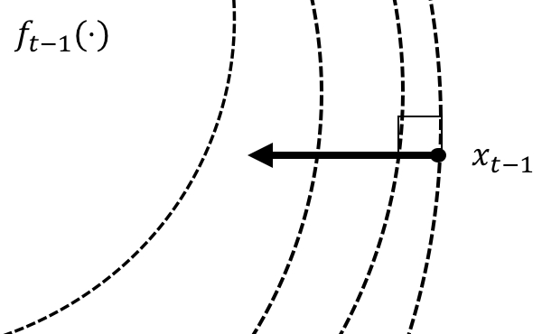
fig:subfigex [A step taken by OMD. Contour lines represent the sub-level sets of $f_{t-1}$.]                          [A step taken by OBD. Contour lines represent the sub-level sets of $f_{t}$.]           

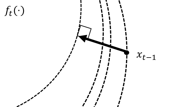
Figure 1: An illustration of the difference between OBD and OMD assuming the mirror map $\Phi(x)=\frac{1}{2}\left\lVert x\right\rVert^{2}_{2}$. While OMD steps in a direction normal to the contour line of $f_{t-1}(\cdot)$ at $x_{t-1}$, OBD  steps in a direction normal to the contour line of $f_{t}(\cdot)$ at $x_{t}$.

For more general switching costs a similar geometric intuition can be obtained using a mirror map $\Phi$ with respect to the norm $\|\cdot\|$. Here, $x_{t}$ is the solution of the following optimization in dual space where, given a convex function $\Phi$, $D_{\Phi}(x,y)$ is the Bregman divergence between $x$ and $y$, i.e., $D_{\Phi}(x,y)=\Phi(x)-\Phi(y)-\nabla\Phi(y)^{T}(x-y)$: minimize  D_Φ(x, x_t-1)   subject to  f_t(x) ≤l. As before, let $\eta_{t}$ be the optimal dual variable for the inequality constraint. The first order optimality condition implies that $x_{t}$ must satisfy

$$\nabla\Phi(x_{t})=\nabla\Phi(x_{t-1})-\eta_{t}\nabla f_{t}(x_{t}).$$ (3)

The form of eqn: mirror-descent-step is similar to a “one step ahead” version of OMD with time varying $\eta_{t}$, i.e., the update direction in the dual space is in the gradient $\nabla f_{t}(x_{t})$ instead of the gradient $\nabla f_{t-1}(x_{t-1})$. The implicit form of the update has been widely used in online learning, e.g., Kivinen and Warmuth (1997); Kulis and Bartlett (2010).

Figure 1 illustrates the difference between OBD and OMD when $\Phi(x)=\frac{1}{2}\left\lVert x\right\rVert^{2}_{2}$: OBD is normal to the destination whereas OMD is normal to the starting point. Intuitively, this is why the guarantees we obtain for OBD are stronger than what previous descent-based approaches have obtained in this setting – it is better to move in the direction determined by the level set where you land, than the direction determined by the level set where you start.

3.2 A Meta Algorithm

The previous section gives intuition about one key aspect of the algorithm, the projection onto a level-set. But, in the discussion above we assume we are projecting onto a specific $l$-sublevel set. The core of OBD is that this sublevel set is determined endogenously in order to “balance” the switching and hitting costs, as opposed to a fixed exogenous schedule of step-sizes like is typical in many online descent algorithms. Informally, the operation of OBD is summarized in the meta algorithm in Algorithm 1, which uses the operator $\Pi^{\Phi}_{K}(x):\mathbb{R}^{n}\rightarrow K$ to denote the Bregman projection of $x$ onto a convex set $K$, i.e., $\Pi^{\Phi}_{K}(x)=\argmin_{y\in K}D_{\Phi}(y,x)$, where $\Phi$ is $m$-strongly convex and $M$-Lipschitz smooth in $\left\lVert\cdot\right\rVert$, i.e., $\frac{m}{2}\left\lVert x-y\right\rVert^{2}\leq D_{\Phi}(x,y)\leq\frac{M}{2}\left\lVert x-y\right\rVert^{2}.$

We term Algorithm 1 a meta algorithm because the general framework given in Algorithm 1 can be instantiated with different forms of “balance” in order to perform well for different metrics. More specifically, the notion of “balance” in the Step 2 that is appropriate varies depending on whether the goal is to perform well for competitive ratio or for regret.

Our results in this paper highlight two different approaches for defining balance in OBD based on either balancing the switching cost with the hitting cost in either the primal or dual space. We balance costs in the primal space to yield a constant, dimension-free competitive algorithm for locally polyhedral cost functions (Section 4), and balance in the dual space to yield a no-regret algorithm (Section 5). We summarize these two approaches in the following and then give more complete descriptions in the corresponding technical sections.

0:  Starting point $x_{0}$, mirror map $\Phi$.

1:  for $t=1,\ldots,T$ do

2:     Choose a sublevel set $K_{l}=\{x\mid f_{t}(x)\leq l\}$ to “balance” the switching and hitting costs.

3:     Set $x_{t}=\Pi^{\Phi}_{K_{l}}(x_{t-1})$.

4:  end for

Algorithm 1 Online Balanced Descent (OBD), Meta Algorithm

• Primal Online Balanced Descent. The algorithm we consider in Section 4 instantiates Algorithm 1 by choosing $l$ such that $x(l)=\Pi^{\Phi}_{K_{l}}(x_{t-1})$ achieves balance between the switching cost with the hitting cost in the primal space. Specifically, for some fixed $\beta>0$, choose $l$ such that either $x(l)=\argmin_{x}f_{t}(x)$ and $\left\lVert x(l)-x_{t-1}\right\rVert<\beta l$, or the following is satisfied:

  $$\left\lVert x(l)-x_{t-1}\right\rVert=\beta l$$ (4)

• Dual Online Balanced Descent. The algorithm we consider in Section 5 instantiates Algorithm 1 by balancing the switching cost with the size of the gradient in the dual space. Specifically, for some fixed $\eta$, we choose $l$ such that

  $$\left\lVert\nabla\Phi(x(l))-\nabla\Phi(x_{t-1})\right\rVert_{*}=\eta\left\lVert\nabla f_{t}(x(l))\right\rVert_{*},$$ (5)

The final piece of the algorithm is computational. Note that the algorithm is memoryless, i.e., it does not use any information about previous cost functions. Thus, the only question about efficiency is whether the appropriate $l$ can be found efficiently. The following lemmas verify that, indeed, it is possible to compute $l$, and thus implement OBD, efficiently.

Lemma 2

The function $g(l)=\left\lVert x(l)-x_{t-1}\right\rVert$ is continuous in $l$.

Lemma 3

Consider $\Phi$ and $f_{t}$ that are continuously differentiable on $\mathcal{X}$. The function
$h(l)=\frac{\left\lVert\nabla\Phi(x_{t-1})-\nabla\Phi(x(l))\right\rVert_{*}}{\left\lVert\nabla{f_{t}(x(l))}\right\rVert_{*}}$ is continuous in $l$.

The continuity of $g(l)$ and $h(l)$ in $l$ is enough to guarantee efficient implementation of Primal and Dual OBD because it shows that an $l$ satisfying the balance conditions in the algorithms exists and, further, can be found to arbitrary precision via bisection. Proofs are included in the appendix.

3.3 Examples

An important part of the design of an OBD algorithm is the choice of the mirror map. Different choices of a mirror map $\Phi$ can lead to very different behavior by the resulting algorithms. To highlight this, and give intuition for the impact of the choice, we describe three examples of mirror maps below. These examples focus on mirror maps that are commonly used for OMD, and they highlight interesting connections between the OBD framework and classical online optimization algorithms like OGD (Zinkevich, 2003) and Multiplicative Weights (Arora et al., 2012).

Euclidean norm squared:

Consider $\Phi(x)=\frac{1}{2}\left\lVert x\right\rVert_{2}^{2}$, which is both 1-strongly convex and 1-Lipschitz smooth for the $\ell_{2}$ norm. Note that $\nabla\Phi(x)=x$. Then, the first order condition eqn: mirror-descent-step is

$$x_{t}=x_{t-1}-\eta_{t}\nabla f_{t}(x_{t}).$$ (6)

Interestingly, this can be interpreted as a “one-step ahead” OGD (illustrated in Figure 1). However, note that this equation should not be interpreted as an update rule since $x_{t}$ appears on both side of the equation. In fact, this contrast highlights an important difference between OGD and OBD.

Mahalanobis distance square:

Consider $\Phi(x)=\frac{1}{2}\left\lVert x\right\rVert_{Q}^{2}$ for positive definite definite $Q$, which is 1-strongly convex and 1-Lipschitz smooth in the Mahalanobis distance $\left\lVert\cdot\right\rVert_{Q}$. Note that $\nabla\Phi(x)=Qx$. Then, the first order condition eqn: mirror-descent-step is

$$x_{t}=x_{t-1}-\eta_{t}Q^{-1}\nabla f_{t}(x_{t}).$$ (7)

This is analogous to a “one step ahead” OGD where the underlying metric is a weighted $\ell_{2}$ metric.

Negative entropy:

If the feasible set is the $\delta$-interior of the simplex $\mathcal{X}=P_{\delta}=\{x\mid\sum_{i=1}^{n}x_{i}=1,x_{i}\geq\delta\}$, and the norm is the $\ell_{1}$ norm $\left\lVert\cdot\right\rVert$, the mirror map defined by the negative entropy $\Phi(x)=\sum_{i=1}^{n}x_{i}\log x_{i}$ is $\frac{1}{2\ln 2}$-strongly convex (by Pinsker’s inequality) and $\frac{1}{\delta\ln 2}$-Lipschitz smooth (by reverse Pinsker’s inequality (Sason and Verdú, 2015)). In this case, $\nabla\Phi(x)=\log x+1_{d}$, where $1_{d}$ represents the all 1s vector in $\mathbb{R}^{d}$. Then, the first order condition is

$$x_{t}=x_{t-1}\exp(-\eta_{t}\nabla f_{t}(x_{t})).$$ (8)

This can be viewed as a “one-step ahead” version of the multiplicative weights update. Again, this equation should not be interpreted as an update rule since $x_{t}$ appears on both side of the equation.

4 A Competitive Algorithm

In this section, we use the OBD framework to give the first algorithm with a dimension-free, constant competitive ratio for online convex optimization with switching costs in general Euclidean spaces, under mild assumptions on the structure of the cost functions. Recall that, for the most general case, where no constraints other than convexity are applied to the cost functions, Proposition 1 shows that the competitive ratio of any online algorithm must be $\Omega(\sqrt{d})$ for $\ell_{2}$ switching costs, i.e., must grow with the dimension $d$ of the decision space. Our goal in this section is to understand when a dimension-free, constant competitive ratio can be obtained. Thus, we are naturally led to restrict the type of cost functions we consider.

Our main result in this section is a new online algorithm whose competitive ratio is constant with respect to dimension when the cost functions are locally polyhedral, a class that includes the form of cost functions used in many applications of online convex optimization, e.g, tracking problems and penalized estimation problems. Roughly speaking, locally polyhedral functions are those that grow at least linearly as one moves away from the minimizer, at least in a small neighborhood.

Definition

A function $f_{t}$ with minimizer $v_{t}$ is locally $\alpha$-polyhedral with respect to the norm $\|\cdot\|$ if there exists some $\alpha,\epsilon>0$, such that for all $x\in\mathcal{X}$ such that $\left\lVert x-v_{t}\right\rVert\leq\epsilon$, $f_{t}(x)-f_{t}(v_{t})\geq\alpha\left\lVert x-v_{t}\right\rVert$.

Note that all strictly convex functions $f_{t}$ which are locally $\alpha$-polyhedral automatically satisfy $f_{t}(x)-f_{t}(v_{t})\geq\alpha\left\lVert x-v_{t}\right\rVert$ for all $x$, not just those $x$ which are $\epsilon$ close to the minimizer $v_{t}$. In this setting, local polyhedrality is analogous to strong convexity; instead of requiring that the cost functions grow at least quadratically as one moves away from the minimizer, the definition requires that cost functions grow at least linearly. The following examples illustrate the breadth of this class of functions. One important class of examples are functions of the form $\|x-v_{t}\|_{a}$ where $\|\cdot\|_{a}$ is an arbitrary norm; it follows from the equivalence of norms that such functions are locally polyhedral with respect to any norm. Intuitively, such functions represent “tracking” problems, where we seek to get close to the point $v_{t}$. Another important example is the class $f(x_{t})=g(x_{t})+h(x_{t})$ where $g$ is locally polyhedral and $h$ is an arbitrary non-negative convex function whose minimizer coincides with that of $g$; since $f(x_{t})-f(v_{t})\geq g(x_{t})-g(v_{t})$, $f$ is also locally polyhedral. This lets us handle interesting functions such as $f(x_{t})=\|x_{t}\|_{1}+x_{t}^{\prime}Qx_{t}$ with $Q$ psd, or even $f(X_{t})=2\|X_{t}\|_{\infty}-\log{\det{\left(I+X_{t}\right)}}$ where the decision variable $X_{t}$ is a PSD matrix. Note that locally polyhedral function have previously been applied in the networking community, e.g., by Huang and Neely (2011) to study delay-throughput trade-offs for stochastic network optimization and by Lin et al. (2012) to design online algorithm for geographical load balancing in data centers.

Let us now informally describe how the Online Balanced Descent framework described in Section 3 can be instantiated to give a competitive online algorithm for locally polyhedral cost functions. Online Balanced Descent is, in some sense, lazy: instead of moving directly towards the minimizer $v_{t}$, it moves to the closest point which results in a suitably large decrease in the hitting cost. This can be interpreted as projecting onto a sublevel set of the current cost function. The trick is to make sure that not too much switching cost is incurred in the process. This is accomplished by carefully picking the sublevel set so that the hitting costs and switching costs are balanced. A formal description is given Algorithm 2. By Lemma 2, step 6 can be computed efficiently via bisection on $l$. Note that the memoryless algorithm proposed in Bansal et al. (2015) can be seen as a special case of Algorithm 2 when the decision variables are scalar.

1:  for $t=1,\ldots,T$ do

2:     Observe cost function $f_{t}$, set $v_{t}=\argmin_{x}f_{t}(x)$.

3:     if $\left\lVert x_{t-1}-v_{t}\right\rVert<\beta f_{t}(v_{t})$ then

4:        Set $x_{t}=v_{t}$

5:     else

6:        Let $x(l)=\Pi_{K_{t}^{l}}^{\Phi}(x_{t-1})$, increase $l$ until $\left\lVert x(l)-x_{t-1}\right\rVert=\beta l$. Here $K_{t}^{l}$ is the $l$-sublevel set of $f_{t}$, i.e., $K_{t}^{l}=\{x\mid f_{t}(x)\leq l\}$.

7:        $x_{t}=x(l)$.

8:     end if

9:  end for

Algorithm 2 (Primal) Online Balanced Descent

The main result of this section is a characterization of the competitive ratio of Algorithm 2.

Theorem 4

For every $\alpha>0$, there exists a choice of $\beta$ such that Algorithm 2 has competitive ratio at most $3+O(1/\alpha)$ when run on locally $\alpha$-polyhedral cost functions with $\ell_{2}$ switching costs. More generally, let $\|\cdot\|$ be an arbitrary norm. There exists a choice of $\beta$ such that Algorithm 2 has competitive ratio at most $\frac{\max\{k_{2},1\}}{\min\{k_{1},1\}}\left(3+O(1/\alpha)\right)$ when run on locally $\alpha$-polyhedral cost functions with switching cost $\|\cdot\|$. Here $k_{1}$ and $k_{2}$ are constants such that $k_{1}\left\lVert x\right\rVert\leq\left\lVert x\right\rVert_{2}\leq k_{2}\left\lVert x\right\rVert$.

We note that in the $\ell_{2}$ setting Theorem 4 has a form which is connected to the best known lower bound on the competitive ratio of memoryless algorithms. In particular, Bansal et al. (2015) use a 1-dimensional example with locally polyhedral cost functions to prove the following bound.

Proposition 5

No memoryless algorithm can have a competitive ratio less than 3.

Beyond the $\ell_{2}$ setting, the competitive ratio in Theorem 4 is no longer dimension-free. It is interesting to note that, when the switching costs are $\ell_{1}$ or $\ell_{\infty}$ and $\alpha$ is fixed, Online Balanced Descent has a competitive ratio that is $O(\sqrt{d})$. In particular, we showed in Section 2 that for general cost functions, there is a $\Omega(d)$ lower bound on the competitive ratio for SOCO with $\ell_{\infty}$ switching costs; hence our $O(\sqrt{d})$ result highlights that local polyhedrality is useful beyond the $\ell_{2}$ case.

While Theorem 4 suggests that Online Balanced Descent has a constant (dimension-free) competitive ratio only in the $\ell_{2}$ setting, a more detailed analysis shows that it can be constant-competitive outside of the $\ell_{2}$ setting as well, though for a more restrictive class of locally polyhedral functions. This is summarized in the the following theorem.

Theorem 6

Let $\|\cdot\|$ be any norm such that the corresponding mirror map $\Phi$ has Bregman divergence $D_{\Phi}$ satisfying $\frac{m}{2}\left\lVert x-y\right\rVert^{2}\leq D_{\Phi}(x,y)\leq\frac{M}{2}\left\lVert x-y\right\rVert^{2}$ for all $x,y\in\mathbb{R}^{d}$ and some positive constants $m$ and $M$. Let $\kappa=M/m$. For every $\alpha>2\sqrt{\kappa-1}$, there exists a choice of $\beta$ so that Algorithm 2 has competitive ratio at most $3+O(1/\alpha)$ when run on locally $\alpha$-polyhedral cost functions with switching costs given by $\|\cdot\|$.

This theorem highlights that for any given locally polyhedral cost functions, the task of finding a constant-competitive algorithm can be reduced to finding an appropriate $\Phi$. In particular, given a class of polyhedral cost functions with $\alpha>0$ and norm $\left\lVert\cdot\right\rVert$, the problem of finding a dimension-free competitive algorithm can be reduced to finding a convex function $\Phi$ that satisfies the differential inequality $\frac{1}{2}\left\lVert x-y\right\rVert^{2}\leq\Phi(x)-\Phi(y)-\langle\nabla\Phi(y),x-y\rangle\leq\frac{\alpha^{2}+4}{8}\left\lVert x-y\right\rVert^{2}$ for all $x,y\in\mathcal{X}$.

We present an intuitive overview of our proof techniques here, and defer the details to the appendix. We use a potential function argument to bound the difference in costs paid by our algorithm and the offline optimal. Our potential function tracks the distance between the points $x_{t}$ picked by our algorithm and the points $x_{t}^{*}$ picked by the offline optimal. There are two cases to consider. Either the online point or the offline point has smaller hit cost. The first case is easy to deal with, since our algorithm is designed so that the movement cost is at most a constant $\beta$ times the hit cost; hence if our online hit cost is less than the offline algorithm’s hit cost, our total per-step cost will at most be a constant times what the offline paid. The second case is more difficult. The key step is Lemma LABEL:lem:_potential-change, where we show that the potential must have decreased if the offline has smaller hit cost. We use this fact to argue that the total per-step cost we charge Online Balanced Descent, namely the sum of the hit cost, movement cost, and change in potential, must be non-positive.

The proof of Theorem 6 parallels that of Theorem 4. The key difference is the use of a more general form of Lemma LABEL:lem:_potential-change, which uses Bregman projection to show that the potential decreases. The Bregman divergence is with respect to the mirror map induced by $\|\cdot\|$.

5 A No-regret Algorithm

1:  for $t=1,\ldots,T$ do

2:     Define $x(l)=\Pi^{\Phi}_{K_{l}}(x_{t-1})$, increase $l$ from $l=f_{t}(v_{t})$, until $\left\lVert\nabla\Phi(x(l))-\nabla\Phi(x_{t-1})\right\rVert_{*}=\eta\left\lVert\nabla f_{t}(x(l))\right\rVert_{*}$.

3:     $x_{t}=x(l)$.

4:  end for

Algorithm 3 (Dual) Online Balanced Descent

While the online algorithms community typically focuses on competitive ratio, regret is typically the focus of the online learning community. The difference in performance metrics leads to differences in the settings considered. In the previous section, we studied locally polyhedral cost functions, while here we focus on cost functions that are continuously differentiable and have a minimizer $v_{t}$ in the interior of the feasible set $\mathcal{X}$.

Interestingly, it is has been shown that the change in metric from competitive ratio to regret has a fundamental impact on the type of algorithms that perform well. Concretely, it has been shown that no single algorithm can perform well across (static) regret and competitive ratio (Andrew et al., 2013). Consequently, it is not surprising that we find a different choice of balance in OBD is needed to obtain the no-regret performance guarantees. Specifically, in contrast to the results of the previous section, which focus on a form of balance in the primal setting, in this section we focus on balance in the dual setting, where we compare costs as measured in the dual norm, $\left\lVert x\right\rVert_{*}=\max_{\left\lVert z\right\rVert\leq 1}\langle z,x\rangle$.

We show that choosing $l$ to balance between the switching cost in the dual space and the size of the gradient leads to an online algorithm with small dynamic regret. It is worth emphasizing that, in contrast to the results of the previous section, we balance the switching cost against the marginal hitting cost $\left\lVert\nabla f_{t}(x_{t})\right\rVert_{*}$ instead of $f_{t}(x_{t})$. A formal description of the instantiation of OBD for regret is given in Algorithm 3, which can be implemented efficiently via bisection (Lemma 3).

Theorem 7

Consider $\Phi$ that is an $m$-strongly convex function in $\left\lVert\cdot\right\rVert$ with $\left\lVert\nabla\Phi(x)\right\rVert_{*}$ bounded above by $G$ and $\nabla\Phi(0)=0$. Then the $L$-constrained dynamic regret of Algorithm 3 is $\leq\frac{GL}{\eta}+\frac{T\eta}{2m}.$

While the result above does not depend on knowing the parameters of the instance, if we know the parameters $T$, $D$ and $L$ ahead of time then we can optimize the balance parameter $\eta$ as follows.

Corollary 8

When $\eta=\sqrt{\frac{2GLm}{T}}$, Algorithm 3 has $L$-constrained dynamic regret $\leq\sqrt{\frac{2GLT}{m}}.$

One interesting aspect of this result is that it has a form similar to the dynamic regret bound on OGD in Theorem 2 of Zinkevich (2003). Both are independent of the dimension of the decision space $d$, assuming the diameter of the space is normalized to $1$. The key difference is that the bound in Corollary 8 is independent of the size of the gradients of the cost functions, unlike in the case of OGD. This can be viewed as a significant benefit that results from the fact that OBD steps in a direction normal to where it lands, rather than where it starts.

Finally, note that Theorem 7 and Corollary 8 additionally provide bounds on the static regret of OBD, by setting $L=D$. In this case, Corollary 8 gives a bound of $O(\sqrt{T})$ which matches the lower bound in the setting where there are no switching costs (Hazan et al., 2016).

Appendix A Lower bounds on competitive ratio and regret

To provide insight as to the difficulty of SOCO, here we give an explicit example that yields lower bounds on the competitive ratio an regret achievable in SOCO. Our example is based on the lower bound example for Convex Body Chasing in Friedman and Linial (1993); it was observed in Antoniadis et al. (2016) that Convex Body Chasing is a special case of SOCO. Starting from the origin, in each round, the adversary examines the $i$-th coordinate of the algorithm’s current action. If this coordinate is negative, the adversary picks the cost function which is the indicator of the hyperplane $x_{i}=1$; similarly, if the coordinate is non-negative, the adversary picks the indicator corresponding to the hyperplane $x_{i}=-1$. Hence our online algorithm is forced to move by at least 1 unit each step, paying a total of at least $d$ cost. The offline optimal, on the other hand, simply moves to the intersection of all these hyperplanes in round 1, paying switching cost $\|(1,1,\ldots 1)\|$, which is $\sqrt{d}$ when the underlying norm is $\ell_{2}$ and $1$ when the norm is $\ell_{\infty}$. Hence the competitive ratio is at least $\sqrt{d}$ in the $\ell_{2}$ setting and $d$ in the $\ell_{\infty}$ setting. Further, the regret is at least $\Omega(d)$ for both the $\ell_{2}$ and $\ell_{\infty}$ settings. Note that while it may appear at first glance that our example requires an adaptive adversary, the same example applies for an oblivious adversary because the online algorithm may be assumed to be deterministic.

Appendix B Proof of Lemma 2

Recall the following Pythagorean inequality satisfied by projection onto convex sets using Bregman divergence as measure of distance given by Bubeck et al. (2015, Lemma 4.1).

Proposition 9

For $x_{t},x_{t-1},K_{l}$ in step 3 of Algorithm 1, for any $y\in K_{l}$, we have

$$D_{\Phi}(x_{t},x_{t-1})+D_{\Phi}(y,x_{t})\leq D_{\Phi}(y,x_{t-1}).$$

In particular, note that when $\Phi$ is the 2-norm squared $\left\lVert\cdot\right\rVert_{2}^{2}$, $x_{t}$, $x_{t-1}$ and $y$ form an obtuse triangle.

Let $h(l)=D_{\Phi}(x(l),x_{t-1})$, we first show that $h(l)$ is convex, hence continuous in $l$, and from there we show that $g(l)$ is continuous in $l$. To begin, we can equivalently write the variational form

$$h(l)=\min_{x}\max_{\lambda\geq 0}D_{\Phi}(x,x_{t-1})+\lambda(f(x)-l).$$

Let $H(x,\lambda,l)=D_{\Phi}(x,x_{t-1})+\lambda(f(x)-l)$, $H$ is affine hence convex in $l$ for any given $x$ and $\lambda$. Since maximization preserves convexity, and because $H$ is jointly convex in $(x,l)$, minimization over $x$ also preserves convexity in $l$, hence $h(l)=\min_{x}\max_{\lambda\geq 0}H(x,\lambda,l)$ is convex hence continuous in $l$. To show $g(l)$ is continuous at $l$, given any $\epsilon>0$, let $\delta>0$ such that $|h(l)-h(l+\delta)|<\epsilon^{2}m/2$ (this can be done as $h$ is continuous in $l$), then — g(l) - g(l+δ) — & ≤x(l) - x(l+δ)
≤2m⋅D_Φ(x(l+δ), x(l))
≤2m⋅(D_Φ(x(l), x_t-1) - D_Φ(x(l+δ), x_t-1))
= 2m⋅— h(l) - h(l+δ)— ¡ ϵ, where the first inequality is due to triangle inequality, and the second inequality is due to the definition of Bregman divergence and $\Phi$ being $m$ strongly convex in $\left\lVert\cdot\right\rVert$, the third inequality is due to the fact that $x(l)\in K_{l+\delta}$ and Proposition 9. Therefore $g$ is a continuous function in $l$.

Appendix C Proof of Lemma 3

First, we will show that $h_{1}(l)=\left\lVert\nabla\Phi(x_{t-1})-\nabla\Phi(x(l))\right\rVert_{*}$ is continuous in $l$. For any $l_{1},l_{2}$, $|h_{1}(l_{1})-h_{1}(l_{2})|\leq\left\lVert\nabla\Phi(x(l_{1}))-\nabla\Phi(x(l_{2}))\right\rVert_{*}$ by the triangle inequality, as $\Phi$ is continuously differentiable, we only need to show that for any $l$, given any $\epsilon>0$, we can find $\delta>0$, such that for all $l^{\prime}$, such that $|l-l^{\prime}|<\delta$, $\left\lVert\nabla\Phi(x(l))-\nabla\Phi(x(l^{\prime}))\right\rVert_{*}<\epsilon$. By Lipschitz smoothness of $\Phi$, we have:

$$D_{\Phi}(x,y)\geq\frac{1}{2M}\left\lVert\nabla\Phi(x)-\nabla\Phi(y)\right\rVert_{*}^{2}.$$ (9)

To show eqn: smoothness-ineq, note that by (Kakade et al., 2009, Theorem 1) $\Phi$ is $M$-Lipschitz smooth w.r.t $\left\lVert\cdot\right\rVert$ if and only if $\Phi^{*}$ is $\frac{1}{M}$-smooth w.r.t $\left\lVert\cdot\right\rVert_{*}$. Let $u=\nabla\Phi(x),v=\nabla\Phi(y)$, then by strong convexity,

$$\Phi^{*}(v)-\Phi^{*}(u)-\langle\nabla\Phi^{*}(u),v-u\rangle\geq\frac{1}{2M}\left\lVert v-u\right\rVert_{*}^{2}.$$ (10)

By the Fenchel inequality and the definition of $u,v$, we have $\Phi^{*}(v)=\langle v,y\rangle-\Phi(y)$ and $\Phi^{*}(u)=\langle u,x\rangle-\Phi(x)$. Furthermore, $\nabla\Phi^{*}(u)=\nabla\Phi^{*}(\nabla\Phi(x))=x$, substituting these into eqn: strong-convex-ineq gives eqn: smoothness-ineq.

Using eqn: smoothness-ineq and Proposition 9, we can upper bound $\left\lVert\nabla\Phi(x(l)-\nabla\Phi(x(l^{\prime})\right\rVert_{*}$ by ∇Φ(x(l)) - ∇Φ(x(l’)) _* &≤2M D_Φ(x(l), x(l’))
≤2M D_Φ(x(l), x_t-1 ) - D_Φ(x(l’), x_t-1) . However, since we have already shown that $D_{\Phi}(x(l),x_{t-1})$ is continuous in $l$ in the proof of Lemma 2, we can choose $l^{\prime}$ sufficiently close to $l$ to make the right hand side smaller than $\epsilon$. Therefore $h_{1}(l)=\left\lVert\nabla\Phi(x_{t-1})-\nabla\Phi(x(l))\right\rVert_{*}$ is continuous in $l$. Second, since $f_{t}$ is also continuously differentiable, and by the continuity of $x(l)$ in $\left\lVert\cdot\right\rVert$, $h_{2}(l)=\left\lVert\nabla f_{t}(x(l))\right\rVert_{*}$ is also continuous in $l$. Thus, the ratio $h(l)=\frac{h_{1}(l)}{h_{2}(l)}$ is continuous in $l$.

Appendix D Proof of Theorem 4

We first consider the case when the switching cost is the $\ell_{2}$ norm. We define $H_{t}=f_{t}(x_{t}),M_{t}=\left\lVert x_{t}-x_{t-1}\right\rVert$, and define $H_{t}^{*}$ and $M_{t}^{*}$ analogously. We use the potential function $\phi(x_{t},x_{t}^{*})=C\left\lVert x_{t}-x_{t}^{*}\right\rVert$; $C$ will end up being the competitive ratio of Algorithm 2. To show Algorithm 2 is $C$-competitive, we need to show that for all $t$,

$$H_{t}+M_{t}+\phi(x_{t},x_{t}^{*})-\phi(x_{t-1},x_{t-1}^{*})\leq C(H_{t}^{*}+M_{t}^{*}),$$ (11)

then summing up the inequality over $t$ implies the result. To begin, applying the triangle inequality, we see

$$\phi(x_{t},x_{t}^{*})-\phi(x_{t-1},x_{t-1}^{*}) \leq C(\left\lVert x_{t}^{*}-x_{t}\right\rVert-\left\lVert x_{t}^{*}-x_{t-1}\right\rVert)+CM_{t}^{*}.$$ (12)

Combining eqn: potential-change and eqn: potential-ineq, we see that, to show Algorithm 2 is $C$-competitive, it suffices to show

References

- Abernethy et al. (2010) Jacob Abernethy, Peter L Bartlett, Niv Buchbinder, and Isabelle Stanton. A regularization approach to metrical task systems. In International Conference on Algorithmic Learning Theory, pages 270–284. Springer, 2010.
- Agrawal et al. (1990) R Agrawal, M Hegde, and D Teneketzis. Multi-armed bandit problems with multiple plays and switching cost. Stochastics and Stochastic Reports, 29(4):437–459, 1990.
- Andrew et al. (2013) Lachlan Andrew, Siddharth Barman, Katrina Ligett, Minghong Lin, Adam Meyerson, Alan Roytman, and Adam Wierman. A tale of two metrics: Simultaneous bounds on competitiveness and regret. In Conference on Learning Theory, pages 741–763, 2013.
- Antoniadis et al. (2016) Antonios Antoniadis, Neal Barcelo, Michael Nugent, Kirk Pruhs, Kevin Schewior, and Michele Scquizzato. Chasing Convex Bodies and Functions, pages 68–81. 2016.
- Arora et al. (2012) Sanjeev Arora, Elad Hazan, and Satyen Kale. The multiplicative weights update method: a meta-algorithm and applications. Theory of Computing, 8(1):121–164, 2012.
- Badiei et al. (2015) Masoud Badiei, Na Li, and Adam Wierman. Online convex optimization with ramp constraints. In IEEE Conference on Decision and Control, pages 6730–6736, 2015.
- Bansal et al. (2015) Nikhil Bansal, Anupam Gupta, Ravishankar Krishnaswamy, Kirk Pruhs, Kevin Schewior, and Clifford Stein. A 2-competitive algorithm for online convex optimization with switching costs. In Approximation, Randomization, and Combinatorial Optimization. Algorithms and Techniques, pages 96–109, 2015.
- Blum and Burch (2000) Avrim Blum and Carl Burch. On-line learning and the metrical task system problem. Machine Learning, 39(1):35–58, Apr 2000.
- Blum et al. (1992) Avrim Blum, Howard Karloff, Yuval Rabani, and Michael Saks. A decomposition theorem and bounds for randomized server problems. In Foundations of Computer Science, pages 197–207, 1992.
- Blum et al. (2002) Avrim Blum, Shuchi Chawla, and Adam Kalai. Static optimality and dynamic search-optimality in lists and trees. In Proc. of ACM-SIAM Symposium on Discrete Algorithms, pages 1–8, 2002.
- Borodin and El-Yaniv (2005) Allan Borodin and Ran El-Yaniv. Online computation and competitive analysis. Cambridge University Press, 2005.
- Borodin et al. (1992) Allan Borodin, Nathan Linial, and Michael E. Saks. An optimal on-line algorithm for metrical task system. J. ACM, 39(4):745–763, October 1992.
- Bubeck et al. (2017) S. Bubeck, M. B. Cohen, J. R. Lee, Y. Tat Lee, and A. Madry. k-server via multiscale entropic regularization. ArXiv e-prints, 2017.
- Bubeck et al. (2015) Sébastien Bubeck et al. Convex optimization: Algorithms and complexity. Foundations and Trends in Machine Learning, 8(3-4):231–357, 2015.
- Buchbinder et al. (2012) Niv Buchbinder, Shahar Chen, Joshep Seffi Naor, and Ohad Shamir. Unified algorithms for online learning and competitive analysis. In Conference on Learning Theory, pages 5–1, 2012.
- Buchbinder et al. (2014) Niv Buchbinder, Shahar Chen, and Joseph Seffi Naor. Competitive analysis via regularization. In Proceedings of the twenty-fifth annual ACM-SIAM symposium on Discrete algorithms, pages 436–444. Society for Industrial and Applied Mathematics, 2014.
- Cesa-Bianchi et al. (2012) Nicolò Cesa-Bianchi, Pierre Gaillard, Gábor Lugosi, and Gilles Stoltz. A new look at shifting regret. CoRR, abs/1202.3323, 2012.
- Chen et al. (2015) Niangjun Chen, Anish Agarwal, Adam Wierman, Siddharth Barman, and Lachlan LH Andrew. Online convex optimization using predictions. In ACM SIGMETRICS Performance Evaluation Review, volume 43, pages 191–204. ACM, 2015.
- Chen et al. (2016) Niangjun Chen, Joshua Comden, Zhenhua Liu, Anshul Gandhi, and Adam Wierman. Using predictions in online optimization: Looking forward with an eye on the past. SIGMETRICS Perform. Eval. Rev., 44(1):193–206, June 2016.
- Friedman and Linial (1993) Joel Friedman and Nathan Linial. On convex body chasing. Discrete & Computational Geometry, 9(3):293–321, Mar 1993.
- Goel et al. (2017) Gautam Goel, Niangjun Chen, and Adam Wierman. Thinking fast and slow: Optimization decomposition across timescales. arXiv preprint arXiv:1704.07785, 2017.
- Guha and Munagala (2009) Sudipto Guha and Kamesh Munagala. Multi-armed bandits with metric switching costs. In International Colloquium on Automata, Languages, and Programming, pages 496–507. Springer, 2009.
- Hall and Willett (2013) Eric C Hall and Rebecca M Willett. Dynamical models and tracking regret in online convex programming. arXiv preprint arXiv:1301.1254, 2013.
- Hazan et al. (2016) Elad Hazan et al. Introduction to online convex optimization. Foundations and Trends in Optimization, 2(3-4):157–325, 2016.
- Herbster and Warmuth (2001) Mark Herbster and Manfred K. Warmuth. Tracking the best linear predictor. Journal of Machine Learning Research, 1:281–309, 2001.
- Huang and Neely (2011) Longbo Huang and Michael J. Neely. Delay reduction via lagrange multipliers in stochastic network optimization. IEEE Transactions on Automatic Control, 56(4):842–857, 2011.
- Joseph and de Veciana (2012) Vinay Joseph and Gustavo de Veciana. Jointly optimizing multi-user rate adaptation for video transport over wireless systems: Mean-fairness-variability tradeoffs. In IEEE INFOCOM, pages 567–575, 2012.
- Kakade et al. (2009) Sham Kakade, Shai Shalev-Shwartz, and Ambuj Tewari. On the duality of strong convexity and strong smoothness: Learning applications and matrix regularization. Manuscript, http://ttic. uchicago. edu/shai/papers/KakadeShalevTewari09.pdf, 2009.
- Kim and Giannakis (2014) Seung-Jun Kim and Geogios B Giannakis. Real-time electricity pricing for demand response using online convex optimization. In IEEE Innovative Smart Grid Tech., pages 1–5, 2014.
- Kim et al. (2015) Taehwan Kim, Yisong Yue, Sarah Taylor, and Iain Matthews. A decision tree framework for spatiotemporal sequence prediction. In ACM International Conference on Knowledge Discovery and Data Mining, pages 577–586, 2015.
- Kivinen and Warmuth (1997) Jyrki Kivinen and Manfred K Warmuth. Exponentiated gradient versus gradient descent for linear predictors. Information and Computation, 132(1):1–63, 1997.
- Koren et al. (2017) Tomer Koren, Roi Livni, and Yishay Mansour. Multi-armed bandits with metric movement costs. In Advances in Neural Information Processing Systems, pages 4122–4131, 2017.
- Kulis and Bartlett (2010) Brian Kulis and Peter L Bartlett. Implicit online learning. In Proceedings of the 27th International Conference on Machine Learning (ICML-10), pages 575–582. Citeseer, 2010.
- Li et al. (2018) Yingying Li, Guannan Qu, and Na Li. Online optimization with predictions and switching costs: Fast algorithms and the fundamental limit. arXiv preprint arXiv:1801.07780, 2018.
- Lin et al. (2011) Minghong Lin, Adam Wierman, Lachlan L. H. Andrew, and Thereska Eno. Dynamic right-sizing for power-proportional data centers. In IEEE INFOCOM, pages 1098–1106, 2011.
- Lin et al. (2012) Minghong Lin, Zhenhua Liu, Adam Wierman, and Lachlan LH Andrew. Online algorithms for geographical load balancing. In IEEE Green Computing Conference, pages 1–10, 2012.
- Lu et al. (2013) Tan Lu, Minghua Chen, and Lachlan LH Andrew. Simple and effective dynamic provisioning for power-proportional data centers. IEEE Transactions on Parallel and Distributed Systems, 24(6):1161–1171, 2013.
- Nemirovskii et al. (1983) Arkadii Nemirovskii, David Borisovich Yudin, and Edgar Ronald Dawson. Problem complexity and method efficiency in optimization. 1983.
- Nesterov (2005) Yu. Nesterov. Smooth minimization of non-smooth functions. Mathematical Programming, 103(1):127–152, May 2005.
- Pruhs (2018) Kirk Pruhs. Errata, 2018. URL http://people.cs.pitt.edu/ kirk/Errata.html.
- Sason and Verdú (2015) Igal Sason and Sergio Verdú. Upper bounds on the relative entropy and rényi divergence as a function of total variation distance for finite alphabets. In IEEE Information Theory Workshop, pages 214–218, 2015.
- Wang et al. (2014) Hao Wang, Jianwei Huang, Xiaojun Lin, and Hamed Mohsenian-Rad. Exploring smart grid and data center interactions for electric power load balancing. ACM SIGMETRICS Performance Evaluation Review, 41(3):89–94, 2014.
- Warmuth and Jagota (1997) Manfred K Warmuth and Arun K Jagota. Continuous and discrete-time nonlinear gradient descent: Relative loss bounds and convergence. In Electronic proceedings of the 5th International Symposium on Artificial Intelligence and Mathematics. Citeseer, 1997.
- Xiao (2010) Lin Xiao. Dual averaging methods for regularized stochastic learning and online optimization. Journal of Machine Learning Research, 11(Oct):2543–2596, 2010.
- Zanini et al. (2009) Francesco Zanini, David Atienza, Luca Benini, and Giovanni De Micheli. Multicore thermal management with model predictive control. In IEEE. European Conf. Circuit Theory and Design, pages 711–714, 2009.
- Zanini et al. (2010) Francesco Zanini, David Atienza, Giovanni De Micheli, and Stephen P Boyd. Online convex optimization-based algorithm for thermal management of MPSoCs. In The Great lakes symposium on VLSI, pages 203–208, 2010.
- Zinkevich (2003) Martin Zinkevich. Online convex programming and generalized infinitesimal gradient ascent. In International Conference on Machine Learning, pages 928–936, 2003.