SPH/$N$-body simulations of small ($D=10\,{\rm km}$) asteroidal breakups and improved parametric relations for Monte–Carlo collisional models

Abstract

We report on our study of asteroidal breakups, i.e. fragmentations of targets, subsequent gravitational reaccumulation and formation of small asteroid families. We focused on parent bodies with diameters $D_{\rm pb}=10\,\rm km$. Simulations were performed with a smoothed-particle hydrodynamics (SPH) code combined with an efficient $N$-body integrator. We assumed various projectile sizes, impact velocities and impact angles (125 runs in total). Resulting size-frequency distributions are significantly different from scaled-down simulations with $D_{\rm pb}=100\,\rm km$ targets (Durda et al., 2007). We derive new parametric relations describing fragment distributions, suitable for Monte-Carlo collisional models. We also characterize velocity fields and angular distributions of fragments, which can be used as initial conditions for $N$-body simulations of small asteroid families. Finally, we discuss a number of uncertainties related to SPH simulations.

1 Introduction and motivation

Collisions between asteroids play an important role in the evolution of the main belt. Understanding the fragmentation process and subsequent reaccumulation of fragments is crucial for studies of the formation of the solar system or the internal structure of the asteroids. Remnants of past break-ups are preserved to a certain extent in the form of asteroid families – groups of asteroids located close to each other in the space of proper elements $a_{\rm p}$, $e_{\rm p}$, $I_{\rm p}$ (Hirayama, 1918; Nesvorný et al., 2015).

The observed size-frequency distribution (SFD) of the family members contains a lot of information and can aid us to determine the mass $M_{\rm PB}$ of the parent body. However, it cannot be determined by merely summing up the observed family members, as a large portion of the total mass is presumably ’hidden’ in fragments well under observational completeness. The SFD is also modified over time, due to ongoing secondary collisional evolution and dynamical removal by the Yarkovsky drift and various gravitational resonances, etc. This makes the procedure a bit difficult for ancient asteroid families and relatively simple for very young ($<10\,\rm Myr$) clusters, such as Karin or Veritas (Nesvorný et al., 2006; Michel et al., 2011).

Disruptive and cratering impacts have been studied experimentally, using impacts into cement mortar targets (e.g. Davis and Ryan, 1990; Nakamura and Fujiwara, 1991). However, in order to compare those results to impacts of asteroids we need to scale the results up in terms of the mass of the target and kinetic energy of the projectile by several orders of magnitude. The scaled impact experiments can still have significantly different outcomes, compared to the asteroid collisions, due to the increasing role of gravitational compression, different fragmentation mechanisms etc. Experiments yield valuable information about properties of materials, but they are not sufficient to unambiguously determine results of asteroid collisions.

Numerical simulations are thus used to solve a standard set of hydrodynamic equations; however, the physics of fragmentation is much more complex than that. Especially for low-energy cratering impacts, it is necessary to simulate an explicit propagation of cracks in the target. There is no ab initio theory of fragmentation, but phenomenological theories has been developed to describe the fragmentation process, such as the Grady–Kipp model of fragmentation (Grady and Kipp, 1980), used in this paper, or more complex models including porosity based on the P-$\alpha$ model (Herrmann, 1969).

Common methods of choice for studying impacts are shock-physics codes and particle codes (Jutzi et al., 2015). The most important outputs of simulations are masses $M_{\rm lr}$ and $M_{\rm lf}$ of the largest remnant and largest fragment, respectively, and the exponent $q$ of the power-law approximation to the cumulative size-frequency distribution $N(>$$D)$, i. e. the number $N$ of family members with diameter larger than given $D$. Parametric relations, describing the dependence of $M_{\rm lr}$ and $q$ on input parameters, can be then applied on collisional models of the main asteroid belt, such as those presented in Morbidelli et al. (2009) or Cibulková et al. (2014); however, if we aim to determine the size of the parent body, we need to solve an inverse problem.

A single simulation gives us the SFD for a given size of the parent body and several parameters of the impactor. However, if one wishes to derive the size of the parent body and impactor parameters from the observed SFD, it is necessary to conduct a large set of simulations with different parameters and then find the SFD that resembles the observed one as accurately as possible. This makes the problem difficult as the parameter space is quite extensive. For one run, we usually have to specify the parent body size $D_{\rm PB}$, the projectile size $d_{\rm project}$, the impact speed $v_{\rm imp}$, and the impact angle $\phi_{\rm imp}$ (i.e. the angle between the velocity vector of the impactor and the inward normal of the target at the point of collision). Other parameters of the problem are the material properties of considered asteroids, such as bulk density, shear modulus, porosity etc.

Due to the extent of the parameter space, a thorough study would be highly demanding on computational resources. It is therefore reasonable to fix the size of the parent body and study breakups with various parameters of the impactor.

A large set of simulations was published by Durda et al. (2007), who studied disruptions of 100 km monolithic targets. Similarly, Benavidez et al. (2012) performed an analogous set of simulations with rubble-pile targets. They also used the resulting SFDs to estimate the size of the parent body for a number of asteroid families. As the diameter of the parent body is never exactly 100 km, the computed SFDs have to be multiplied by a suitable scaling factor $f_{\rm scale}$ to match the observed one. However, small families have been already discovered (e.g. Datura, Nesvorný et al. (2015)) and their parent-body size is likely $D_{\rm pb}=10\,\rm km$, i.e. an order-of-magnitude smaller. The linearity of the scaling is a crucial assumption and we will assess the plausibility of this assumption in this paper.

To fill up a gap in the parameter space, we proceed with small targets. We carried out a set of simulations with $D_{\rm pb}=10\,\rm km$ parent bodies and carefully compared them with the simulations of Durda et al. (2007).

The paper is organised as follows. In Section 2, we briefly describe our numerical methods. The results of simulations are presented in Section 3. Using the computed SFDs we derive parametric relations for the slope $q$ and the masses $M_{\rm lr}$ and $M_{\rm lf}$ of the largest remnant and the largest fragment, respectively, in Section 4. Finally, we summarize our work in Section 5.

2 Numerical methods

We follow a hybrid approach of Michel et al. (2001, 2002, 2003, 2004), employing an SPH discretization for the simulation of fragmentation and an $N$-body integrator for subsequent gravitational reaccumulation. Each simulation can be thus divided into three phases: i) a fragmentation, ii) a hand-off, and iii) a reaccumulation. We shall describe them sequentially in the following subsections.

2.1 Fragmentation phase

The first phase of the collision is described by hydrodynamical equations in a lagrangian frame. They properly account for supersonic shock wave propagation and fragmentation of the material. We use the SPH5 code by Benz and Asphaug (1994) for their numerical solution. In the following, we present only a brief description of equations used in our simulations and we refer readers to extensive reviews of the method (Rosswog, 2009; Cossins, 2010; Price, 2008, 2012) for a more detailed description.

Our problem is specified by four basic equations, namely the equation of continuity, equation of motion, energy equation and Hooke’s law:

$${{\rm d}\rho\over{\rm d}t} = -\rho\nabla\cdot\bm{v}\,,$$ (1)

$${{\rm d}\bm{v}\over{\rm d}t} = {1\over\rho}\nabla\cdot\bm{\sigma}\,,$$ (2)

$${{\rm d}U\over{\rm d}t} = -{P\over\rho}{\rm Tr\,}\dot{\bm{\epsilon}}+{1\over\rho}\bm{S}:\dot{\bm{\epsilon}}\,,$$ (3)

$${{\rm d}\bm{S}\over{\rm d}t} = 2\mu\left(\dot{\bm{\epsilon}}-{\textstyle{1\over 3}}\bm{1}\,{\rm Tr\,}\dot{\bm{\epsilon}}\,\right)\,,$$ (4)

supplemented by the Tillotson equation of state (Tillotson, 1962). The notation is as follows: $\rho$ is the density, $\bm{v}$ the speed, $\bm{\sigma}$ the stress tensor (total), where $\bm{\sigma}\equiv-P\bm{1}+\bm{S}$, $P$ the pressure, $\bm{1}$ the unit tensor, $\bm{S}$ the deviatoric stress tensor, $U$ the specific internal energy, $\dot{\bm{\epsilon}}$ the strain rate tensor, where $\dot{\bm{\epsilon}}\equiv{\textstyle{1\over 2}}\left[\nabla\bm{v}+(\nabla\bm{v})^{\rm T}\right]$, with its trace ${\rm Tr\,}\dot{\bm{\epsilon}}=\nabla\cdot\bm{v}$, $\mu$ the shear modulus.

The model includes both elastic and plastic deformation, namely the yielding criterion of von Mises (1913) — given by the factor $f\equiv\min[Y_{0}^{2}/({3\over 2}\bm{S}:\bm{S}),1]$ — and also failure of the material. The initial distribution of cracks and their growth to fractures is described by models of Weibull (1939) and Grady and Kipp (1980), which use a scalar parameter ${\cal D}\in\langle 0,1\rangle$ called damage, as explained in Benz and Asphaug (1994). The stress tensor of damaged material is then modified as $\bm{\sigma}=-(1-{\cal D}H(-P))P\bm{1}+(1-{\cal D})f\bm{S}$, where $H(x)$ denotes the Heaviside step function. In this phase, we neglect the influence of gravity, which is a major simplification of the problem.

In a smoothed-particle hydrodynamic (SPH) formalism, Eqs. (1) to (4) are rewritten so as to describe an evolution of individual SPH particles (denoted by the index $i=1..N$):

$${{\rm d}\rho_{i}\over{\rm d}t} = -\rho_{i}\sum_{j}\frac{m_{j}}{\rho_{j}}(\bm{v}_{j}-\bm{v}_{i})\cdot\nabla W_{ij}\,,$$ (5)

$${{\rm d}\bm{v}_{i}\over{\rm d}t} = \sum_{j}m_{j}\left(\frac{\bm{\sigma}_{i}+\bm{\sigma}_{j}}{\rho_{i}\rho_{j}}\right)\cdot\nabla W_{ij}\,,$$ (6)

$${{\rm d}U_{i}\over{\rm d}t} = -{P_{i}\over\rho_{i}}\sum_{\gamma}\dot{\epsilon}_{i}^{\gamma\gamma}+{1\over\rho_{i}}\sum_{\alpha}\sum_{\beta}S_{i}^{\alpha\beta}\dot{\epsilon}_{i}^{\alpha\beta}\,,$$ (7)

$${{\rm d}\bm{S}_{i}\over{\rm d}t} = 2\mu\left(\dot{\bm{\epsilon}}_{i}-{\textstyle{1\over 3}}\bm{1}\sum_{\gamma}\dot{\epsilon}_{i}^{\gamma\gamma}\right)\,,$$ (8)

with:

$$\dot{\epsilon}_{i}^{\alpha\beta}={1\over 2\rho_{i}}\sum_{j}m_{j}\left[(v_{j}^{\alpha}-v_{i}^{\alpha}){\partial W_{ij}\over\partial x^{\beta}}+(v_{j}^{\beta}-v_{i}^{\beta}){\partial W_{ij}\over\partial x^{\alpha}}\right]\,,$$ (9)

where $m_{j}$ denote the masses of the individual SPH particles, $W_{ij}\equiv W(|\bm{r}_{i}-\bm{r}_{j}|,h)$ the kernel function, $h$ the symmetrized smoothing length, $h={1\over 2}(h_{i}+h_{j})$. Both the equation of motion and the energy equation were also supplied with the standard artificial viscosity term $\Pi_{ij}$ (Monaghan and Gingold, 1983):

$$\Pi_{ij}=\left\{\begin{array}[]{ll}\frac{1}{\rho}\left(-\alpha c_{\rm s}\mu_{ij}+\beta\mu_{ij}^{2}\right)&(\bm{v}_{i}-\bm{v}_{j})\cdot(\bm{r}_{i}-\bm{r}_{j})\leq 0\,,\\ 0&\rm otherwise\,,\end{array}\right.$$ (10)

where:

$$\mu_{ij}=\frac{h(\bm{v}_{i}-\bm{v}_{j})\cdot(\bm{r}_{i}-\bm{r}_{j})}{\|\bm{r}_{i}-\bm{r}_{j}\|^{2}+\epsilon h^{2}}\,,$$ (11)

$c_{\rm s}$ is the sound speed, $\alpha_{\rm AV}=1.5$ and $\beta_{\rm AV}=3$. We sum over all particles, but since the kernel has a compact support, the algorithm has an asymptotic complexity ${\cal O}(NN_{\rm neighbours})$. The actual number of SPH particles we used is $N\doteq 1.4\times 10^{5}$, and the number of neighbours is usually $N_{\rm neighbours}\simeq 50$. There is also an evolution equation for the smoothing length $h_{i}$ in order to adapt to varying distances between SPH particles.

2.2 Hand-off procedure

Although SPH is a versatile method suitable for simulating both the fragmentation and the gravitational reaccumulation, the time step of the method is bounded by the Courant criterion and the required number of time steps for complete reaccumulation is prohibitive. In order to proceed with inevitably simplified but efficient computations, we have to convert SPH particles to solid spheres, a procedure called hand-off. In this paper, we compute the corresponding radius $R_{i}$ as:

$$R_{i}=\left({3m_{i}\over 4\pi\rho_{i}}\right)^{1\over 3}\,.$$ (12)

The time $t_{\rm handoff}$ at which the hand-off takes place is determined by three conditions:

1. It has to be at least $2D_{\rm PB}/c_{\rm s}\simeq 1\,{\rm s}$ ($c_{\rm s}$ being the sound speed), i.e. until the shock wave and rarefaction wave propagate across the target;

2. Fractures (damage) in the target should not propagate anymore, even though in catastrophic disruptions the shock wave usually damages the whole target and material is then practically strengthless;

3. The pressure in the fragmented parent body should be zero so that the corresponding acceleration $-{1\over\rho}\nabla P$ is zero, or at least negligible. According to our tests for $D_{\rm PB}=10\,{\rm km}$ targets, such relaxation takes up to $10\,{\rm s}$.

On the other hand, there is an upper limit for $t_{\rm handoff}$ given by the gravitational acceleration of the target, $g=GM_{\rm PB}/R_{\rm PB}^{2}$, which has to be small compared to the escape speed $v_{\rm esc}=\sqrt{2GM_{\rm PB}/R_{\rm PB}}$, i.e. a typical ejection speed $v_{\rm ej}$ of fragments. The corresponding time span should thus be definitely shorter than $v_{\rm esc}/g\simeq 10^{3}\,{\rm s}$.

2.3 Reaccumulation phase

Finally, gravitational reaccumulation of now spherical fragments is computed with an $N$-body approach. We use the pkdgrav code as modified by Richardson et al. (2000) for this purpose. It accounts for mutual gravitational interactions between fragments:

$$\ddot{\bm{r}_{i}}=-\sum_{j\neq i}{Gm_{j}\over r_{ij}^{3}}\bm{r}_{ij}\,,$$ (13)

An ${\cal O}(N^{2})$ problem is simplified significantly using a tree code algorithm, i.e. by clustering fragments to cells and evaluating gravitational moments up to hexadecapole order, provided they fit within the opening angle ${\rm d}\theta=0.5\,{\rm rad}$. The time step was $\Delta t=10^{-6}$ (in $G=1$ units, or about $5\,{\rm s}$ in SI), and the time span $50,000\,\Delta t$, long enough that the reaccumulation is over, or negligible.

Regarding mutual collisions, we assumed perfect sticking only, meaning no bouncing or friction. Consequently, we have no information about resulting shapes of fragments, we rather focus on their sizes, velocities and corresponding statistics.

3 A grid of simulations for $D_{\rm PB}=10\,{\rm km}$ targets

We performed a number of simulations with $D_{\rm pb}=10\,\rm km$ parent bodies, impact speed $v_{\rm imp}$ varying from 3 to $7\,\rm km/s$, diameter $d_{\rm project}$ of the impactor from $0.293\,\rm km$ to $1.848\,\rm km$ (with a logarithmic stepping) and the impact angle $\phi_{\rm imp}$ from $15^{\circ}$ to $75^{\circ}$. The kinetic energy of the impact:

$$Q=\frac{\frac{1}{2}m_{\rm project}v_{\rm imp}^{2}}{M_{\rm pb}}$$ (14)

therefore varies from $\sim 10^{-2}Q_{\rm D}^{\star}$ to $\sim 20Q_{\rm D}^{\star}$, where $Q_{\rm D}^{\star}$ is the critical energy for shattering and dispersing 50% of the parent body. We adopted $Q_{\rm D}^{\star}(D)$ values for comparisons from the scaling law of Benz and Asphaug (1999). The total number of performed runs is 125. We assume a monolithic structure of both the target and the impactor, and the material properties were selected those of basalt (summarized in Table 1).

Material parameters
density at zero pressure	$\rho=2700\,\rm kg/m^{3}$
bulk modulus	$A=2.67\cdot 10^{10}\,\rm Pa$
non-linear Tillotson term	$B=2.67\cdot 10^{10}\,\rm Pa$
sublimation energy	$u_{0}=4.87\cdot 10^{8}\,\rm J/kg$
energy of incipient vaporization	$u_{\rm iv}=4.72\cdot 10^{6}\,\rm J/kg$
energy of complete vaporization	$u_{\rm cv}=1.82\cdot 10^{7}\,\rm J/kg$
shear modulus	$\mu=2.27\cdot 10^{10}\,\rm Pa$
von Mises elasticity limit	$Y_{0}=3.50\cdot 10^{9}\,\rm Pa$
Weibull coefficient	$k=4.00\cdot 10^{29}$
Weibull exponent	$m=9$
SPH parameters
number of particles in target	$N_{\rm pb}=10^{5}$
number of particles in projectile	$N_{\rm pb}=100\mbox{ to }630$
Courant number	$C=1$
linear term of artificial viscosity	$\alpha_{\rm AV}=1.5$
quadratic term of artificial viscosity	$\beta_{\rm AV}=3.0$
duration of fragmentation phase	$t_{\rm handoff}=10\,\rm s$

Table 1: Constant parameters used in our SPH simulations.

3.1 Size-frequency distributions

For each run we constructed a cumulative size-frequency distributions $N(>$$D)$ of fragments and we plotted them in Fig. 1.

At first sight, the SFDs are well-behaved. Both cratering and catastrophic events produce mostly power-law-like distributions. Some distributions, mainly those around $Q/Q_{\rm D}^{\star}\sim 1$, have an increasing slope at small sizes (at around $D\sim 0.3\,\rm km$), but since this is close to the resolution limit, it is possibly a numerical artifact.

For supercatastrophic impacts with $d_{\rm project}=1.848\,\rm km$, the distributions differ from power laws substantially; the slope becomes much steeper at large sizes of fragments. These are the cases where the gap between the largest remnant and the largest fragment disappears (we therefore say the largest remnant does not exist).

The situation is quite different for impacts with an oblique impact angle, mainly for $\phi_{\rm imp}=75^{\circ}$. We notice that these impacts appear much less energetic compared to other impact angles, even though the ratio $Q/Q_{\rm D}^{\star}$ is the same. The cause of this apparent discrepancy is simply the geometry of the impact. At high impact angles, the impactor does not hit the target with all its cross-section and a part of it misses the target entirely (grazing impacts, see Leinhardt and Stewart, 2012). Therefore, a part of the kinetic energy is not deposited into the target and the impact appears less energetic, compared to head-on impacts.

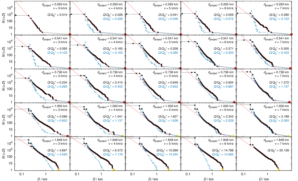
Figure 1: Cumulative size-frequency distributions $N({>}D)$ of fragments ejected during disruptions of parent bodies with sizes $D_{\rm PB}=10\,{\rm km}$. The impact angle was $\phi_{\rm imp}=45^{\circ}$; results for different impact angles are shown in Appendix D. The projectile size is increasing downwards, from $d_{\rm project}=0.293\,\rm km$ to $1.848\,\rm km$, so that the logarithm of the mass ratio $\log_{10}(m_{\rm project}/M_{\rm PB})=3.0,2.6,2.2,1.8$ and $1.0$. The impact speed is increasing to the right, from $v_{\rm imp}=3$ to $7\,{\rm km}\,{\rm s}^{-1}$. Both of the quantities are also indicated in individual panels, together with the ratio $Q/Q^{\star}_{\rm D}$ of the specific energy $Q$ and strength $Q^{\star}_{\rm D}$ inferred from the scaling law of Benz and Asphaug (1999). Largest remnant size $D_{\rm LR}$ is coloured red or yellow for cratering or catastrophic events, respectively. For a discussion of scaling we overplot simulated SFD’s from Durda et al. (2007) computed for disruptions of $D_{\rm PB}=100\,{\rm km}$ targets and scaled down by dividing sizes by a factor of 10 (blue lines and labels). To compare ‘apples with apples’, we compare runs with (approximately) the same $Q/Q^{\star}_{\rm D}$ ratios and the same impact angle. For some impact parameters, the scaled SFD is missing as there is no run in the dataset of Durda et al. (2007) with comparable $Q/Q_{\rm D}^{\star}$. Finally, the red curves are fits of a suitable function, used to derive parametric relations (see Section 4).

3.2 Speed histograms

Similarly to the size-frequency distributions, we computed speed distributions of fragments. The results are shown in Fig. 2. As we are computing an absolute value of the velocity, the resulting histogram depends on a selected reference frame. We chose a barycentric system for all simulations; however, we excluded high-speed remainders of the projectile with velocities $v_{\rm ej}>v_{\rm cut}\equiv 1\,\rm km/s$. These outliers naturally appear mainly for oblique impact angles. Because of very large ejection velocities, such fragments cannot belong to observed families and if we had included them in the constructed velocity field of the synthetic family, it would artificially shift velocities of fragments to higher values.

The main feature of cratering events is the peak around the escape velocity $v_{\rm esc}$. This peak is created by fragments ejected at the point of impact. With an increasing impact energy, the tail of the histogram extends as the fragments are ejected at higher velocities.

Interestingly, there is a second peak at around $Q/Q_{\rm D}^{\star}\sim 0.3$. This is because of ejection of fragments from the antipode of the target. If the shockwave is energetic enough, it causes an ejection of many fragments. The second peak is barely visible at oblique impact angles.

Figure 2: Differential histograms ${\rm d}N$ of ejection speeds $v_{\rm ej}$ of fragments for the same set of simulations as in Fig. 10. The speed is computed in a barycentric reference frame with outliers ($v_{\rm imp}>1\,\rm km/s$) are removed as they are mostly remnants of the projectile. The escape speed from the target $D_{\rm PB}=10\,{\rm km}$ in size is $v_{\rm esc}=6.1\,{\rm m}\,{\rm s}^{-1}$, histogram peaks are thus of order $v_{\rm esc}$, at least for the majority of simulations. However, there is also a significant second peak visible. It is close to the first peak for cratering to mid-energy impacts and extends to speeds $v_{\rm ej}>100\,\rm m/s$ for supercatastrophic breakups with $Q/Q^{\star}_{\rm D}\gtrsim 10$. The impact angle $\phi_{\rm imp}=45^{\circ}$ in this case.

3.3 Isotropy vs anisotropy of the velocity field

Fig. 3 shows angular distributions of the velocity fields in the plane of the impact. The histograms are drawn as polar plots with a $5^{\circ}$ binning. The angles on plots correspond to the points of impact for given impact angle $\phi_{\rm imp}$; for cratering events, all the ejecta are produced at the point of impact and the distribution of fragments is therefore nicely clustered around $\phi_{\rm imp}$.

Cratering impacts tend to produce velocity fields mainly in the direction of the impact angle. Catastrophic impacts, on the other hand, generally produce much more isotropic velocity fields. However, the isotropy is not perfect, even though we removed outliers as above. Even for the supercatastrophic impacts, the number of fragments in different directions can vary by a factor of 5. Further changes of the reference frame may improve the isotropy. Note that for observed families, it is also not clear where is the reference points, as the identification of family members (and interlopers) is ambiguous.

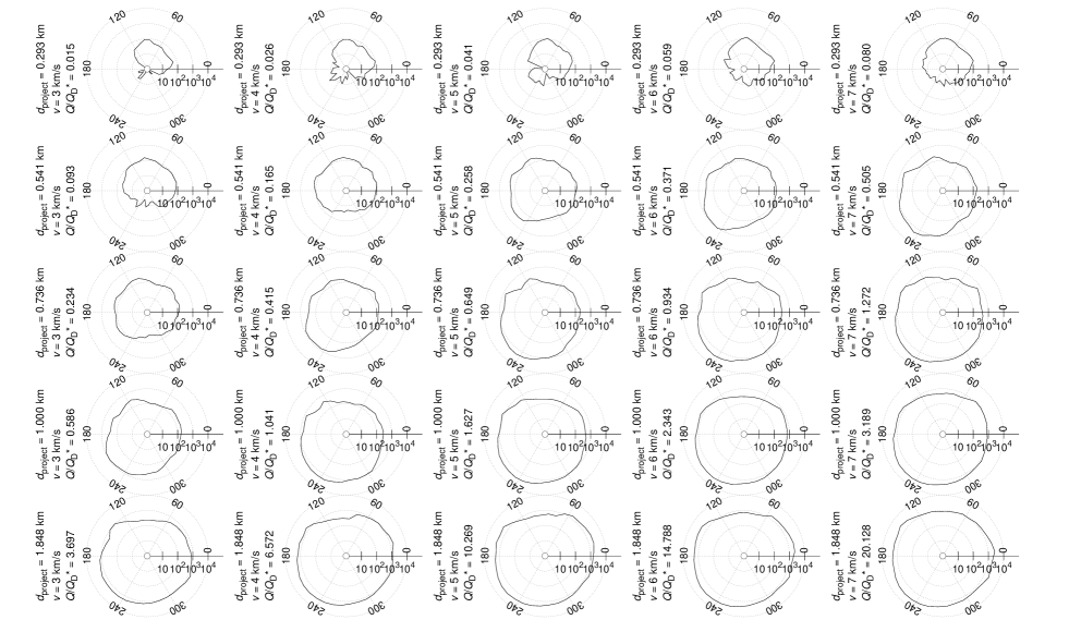
Figure 3: Histograms of velocity angular distribution (in the plane of the collision) of fragments. The velocities are evaluated in the barycentric coordinate system with outliers removed. The angle $180^{\circ}$ corresponds to the velocity direction of the projectile. The impact angle $\phi_{\rm imp}=45^{\circ}$.

3.4 A comparison with scaled-down $\it D_{\rm PB}=100\,{\it km\/}$ simulations

The mid-energy events with $Q/Q_{\rm D}^{\star}\sim 1$ have SFDs comparable to scaled 100 km ones. In this regime, down-scaling of the distribution for $D_{\rm pb}=100\,\rm km$ targets seems to be a justifiable way to approximate SFDs for targets of smaller sizes.

In case of cratering events, however, our simulations differ significantly from scaled ones. Impacts into 10 km targets produce a much shallower fragment distribution compared to 100 km impacts; see impacts with $d_{\rm project}=0.293\,\rm km$. We also note that supercatastrophic runs have different outcomes than the 100 km ones; our distributions are much shallower and have a much larger largest fragment. They also have a steeper part of the SFD at larger diameters, which is not visible for 100 km simulations, at least not to the same extent.

4 Parametric relations for Monte-Carlo collisional models

Size-frequency distributions constructed from our simulations mostly have a power-law shape with a separated largest remnant. The slope of the distribution in a log-log plot can be therefore fitted with a linear function:

$$\log N(>\!D)=q\log[D]_{\rm km}+c\,.$$ (15)

Supercatastrophic events behave differently though, and their SFDs can be well fitted with a two-slope function:

$$\log N(>\!D)=K\left(\log[D]_{\rm km}-\log[D_{0}]_{\rm km}\right)+c\,,$$ (16)

where:

$$K(x)=\frac{1}{2}(q_{1}+q_{2})x+\frac{1}{2}\frac{q_{1}-q_{2}}{k}\log\left(2\cosh kx\right)\,.$$ (17)

In this approximation of the SFD, $q_{1}$ and $q_{2}$ are the limit slopes for $D\rightarrow\infty$ and $D\rightarrow 0$, respectively, and $k$ characterizes the “bend-off“ of the function. As the fitting function is highly non-linear and the dependence on $k$ is very weak (given rather sparse input data), the fit doesn’t generally converge, we thus fix $k=10$ and perform the fit using only four parameters: $s_{1},s_{2},D_{0}$ and $c$.

Because impacts at high angles appear weaker due the geometry (see Section 3.1), we have to account for the actual kinetic energy delivered into the target. We chose a slightly different approach than Leinhardt and Stewart (2012) and modified the specific impact energy $Q$ by a ratio of the cross-sectional area of the impact and the total area of the impactor. Using a formula for circle-circle intersection: let $R$ be the radius of the target, $r$ the radius of the projectile and $d$ a projected distance between their centers. The area of impact is then given by:

$$A =r^{2}\cos^{-1}\left(\frac{d^{2}+r^{2}-R^{2}}{2dr}\right)+R^{2}\cos^{-1}\left(\frac{d^{2}+R^{2}-r^{2}}{2dR}\right)-$$

$$-\frac{1}{2}\sqrt{(R+r-d)(d+r-R)(d-r+R)(d+r+R)}\,.$$ (18)

As both spheres touch at the point of the impact, we have:

$$d=(r+R)\sin\phi_{\rm imp}\,.$$ (19)

Using these auxiliary quantities, we define the effective specific impact energy:

$$Q_{\rm eff}=Q\frac{A}{\pi r^{2}}\,.$$ (20)

In Fig. 4, we separately plot slopes $q$, constants $c$ of the linear fits of the SFDs, and the masses of the largest remnants $M_{\rm lr}$ and largest fragment $M_{\rm lf}$. Each of these quantities shows a distinct dependence on the impact speed $v_{\rm imp}$, suggesting parametric relations cannot be well described by a single parameter $Q_{\rm eff}/Q_{\rm D}$. We therefore plot each dependence separately for different $v_{\rm imp}$ and we explicitly express the dependence on $v_{\rm imp}$ in parametric relations.

For low speeds, slopes $q$ can be reasonably fitted with a function:

$$q=-12.3+0.75v_{\rm imp}+\cfrac{(11.5-1^{+0.2}_{-0.1}v_{\rm imp})\exp\left(-5\cdot 10^{-3}\cfrac{Q_{\rm eff}}{Q_{\rm D}^{\star}}\right)}{1+0.1^{+0.01}_{-0.02}\left(\cfrac{Q_{\rm eff}}{Q_{\rm D}^{\star}}\right)^{-0.4}}\,,$$ (21)

where $v_{\rm imp}$ is expressed in $\rm km/s$. However, for high speeds (especially for $v=7\,\rm km/s$), the individual values of $q$ for different impact angles differ significantly and thus the fit has a very high uncertainty. We account for this behaviour in Eq. (21), where the uncertainty increases with an increasing speed.

The constant $c$ can be well fitted by linear function:

$$c=0.9+2.3\exp(-0.35v_{\rm imp})+\left(1.3-0.1v_{\rm imp}\right)\left(\frac{Q_{\rm eff}}{Q_{\rm D}^{\star}}\right)\,.$$ (22)

The high scatter noted in the parametric relation for the slope $q$ is not present here. This parameter is of lesser importance for Monte-Carlo models though, as the distribution must be normalized anyway to conserve the total mass.

Largest remnants are also plotted in Fig. 4. Notice that some points are missing here as the largest remnant does not exist for supercatastrophic impacts. As we are using the effective impact energy $Q_{\rm eff}$ as an independent variable, the runs with impact angle $\phi=75^{\circ}$ produce largest remnants of sizes comparable to other impact angles. This helps to decrease the scatter of points and make the derived parametric relation more accurate. We selected a fitting function:

$$M_{\rm lr}=\frac{M_{\rm tot}}{1+\left[0.6^{+0.5}_{-0.2}+56\exp(-1.0^{+0.6}_{-0.2}v_{\rm imp})\right]\left(\cfrac{Q_{\rm eff}}{Q_{\rm D}^{\star}}\right)^{0.8+8\exp(-0.7v_{\rm imp})}}\,.$$ (23)

Largest fragments (fourth row) exhibit a larger scatter, similarly as the slopes $q$. The masses of the largest fragment can differ by an order of magnitude for different impact angles (notice the logarithmic scale on the $y$-axis). Nevertheless, the values averaged over impact angles (red circles) lie close the fit in most cases. The fitting function for the largest remnant is:

$$M_{\rm lf}=\frac{M_{\rm tot}}{0.24^{+0.60}_{-0.15}v_{\rm imp}^{3}\left(\cfrac{Q_{\rm eff}}{Q_{\rm D}^{\star}}\right)^{-0.6-2\exp(-0.3v_{\rm imp})}\kern-40.0pt+\exp\left(-0.3^{+0.2}_{-0.2}v_{\rm imp}\right)\cfrac{Q_{\rm eff}}{Q_{\rm D}^{\star}}+11^{+15}_{-8}+2v_{\rm imp}}\,.$$ (24)

This function bends and starts to decrease for $Q/Q_{\rm D}^{\star}\gg 1$. Even though this behaviour is not immediately evident from the plotted points, the largest fragment must become a decreasing function of impact energy in the supercatastrophic regime.

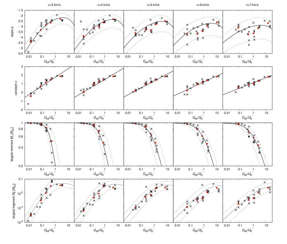
Figure 4: Parameters of the power-law fits of size-frequency distributions (first and second row) and masses of the largest remnant $M_{\rm lr}$ and the largest fragment $M_{\rm lf}$ (third and fourth row) as functions of the effective impact energy $Q_{\rm eff}/Q_{\rm D}^{\star}$, defined by Eq. (20). We plotted these quantities for each value of impact speed separately as considering $Q_{\rm eff}/Q_{\rm D}^{\star}$ as a single parameter would imply a large variance of data and therefore a large uncertainty of parametric relations. Each black cross represents one SPH/$N$-body simulation, and the red circles are given by averaging over impact angles $\phi_{\rm imp}$. The data are fitted with suitable functions and the scatter of values propagates to the parametric relations as uncertainties, (see Section 4).

5 Conclusions and future work

In this paper, we studied disruptions and subsequent gravitational reaccumulation of asteroids with diameter $D_{\rm pb}=10\,\rm km$. Using an SPH code and an efficient $N$-body integrator, we performed impact simulations for various projectile sizes $d_{\rm project}$, impact speeds $v_{\rm imp}$ and angles $\phi_{\rm imp}$. The size-frequency distributions, constructed from the results of our simulations, appear similar to the scaled-down simulations of Durda et al. (2007) only in the transition regime between cratering and catastrophic events ($Q/Q_{\rm D}^{\star}\simeq 1$); however, they differ significantly for both the weak cratering impacts and for supercatastrophic impacts.

The resulting size-frequency distributions can be used to estimate the size of the parent body, especially for small families. As an example, we used our set of simulations to determine $D_{\rm pb}$ of the Karin family. This cluster was studied in detail by Nesvorný et al. (2006) and we thus do not intend to increase the accuracy of their result, but rather to assess the uncertainty of linear SFD scaling. The closest fit to the observed SFD of the Karin cluster yields a parent body with $D_{\rm pb}=25\,\rm km$ — a smaller, but comparable value to $D_{\rm pb}=33\,\rm km$, obtained by Nesvorný et al. (2006). Using the set of $D_{\rm pb}=100\,\rm km$ simulations, Durda et al. (2007) obtained an estimate $D_{\rm pb}\simeq 60\,\rm km$. It is therefore reasonable that the best estimate is intermediate between the result from upscaled 10 km runs and downscaled 100 km runs. We do not consider our result based on “generic” simulations more accurate than the result of Nesvorný et al. (2006); however, the difference between the results can be seen as an estimate of uncertainty one can expect when scaling the SFDs by a factor of 3.

We derived new parametric relations, describing the masses $M_{\rm lr}$ and $M_{\rm lf}$ of the largest remnant and the largest fragment, respectively, and the slope $q$ of the size-frequency distribution as functions of the impact parameters. These parametric relations can be used straightforwardly to improve the accuracy of collisional models, as the fragments created by a disruption of small bodies were previously estimated as scaled-down disruptions of $D_{\rm pb}=100\,\rm km$ bodies.

In our simulations, we always assumed monolithic targets. The results can be substantially different for porous bodies, though, as the internal friction has a significant influence on the fragmentation (Jutzi et al., 2015; Asphaug et al., 2015). This requires using a different yielding model, such as Drucker–Prager criterion. We postpone a detailed comparison between monolithic and porous bodies for future work.

Appendix A Initial distribution of SPH particles

For a unique solution of evolutionary differential equations, initial conditions have to be specified. In our case, this means setting the initial positions and velocities of SPH particles. We assume non-rotating bodies, all particles of the target are therefore at rest and all particles of the impactor move with the speed of the impactor.

Optimal initial positions of SPH particles have to meet several criteria. First of all, the particles have to be distributed evenly in space. This requirement eliminates a random distribution as a suitable method, for using such a distribution would necessarily lead to clusters of particles in some parts of space and a lack of particles in other parts.

We therefore use a hexagonal-close-packing lattice in the simulations. They are easily set up and have an optimal interpolation accuracy. However, no lattice is isotropic, so there are always preferred directions in the distribution of SPH particles. This could potentially lead to numerical artifacts, such as pairing instability (Herant, 1994). Also, since the particle concentration is uniform, the impact is therefore resolved by only a few SPH particles for small impactors. We can increase accuracy of cratering impacts by distributing SPH particles nonuniformly, putting more particles at the point of impact and fewer in more distant places.

Here we assess the uncertainty introduced by using different initial conditions of SPH particles. A suitable method for generating a nonuniform isotropic distribution has been described by Diehl et al. (2012) and Rosswog (2015). Using initial conditions generated by this method, we ran several SPH/$N$-body simulations, and we compared the results to the simulations with lattice initial conditions.

The comparison is in Fig. 5. Generally, the target shatters more for the nonuniform distribution. The largest remnant is smaller; the difference is up to 10% for the performed simulations. There are also more fragments at larger diameters, compared to the lattice distribution. This is probably due to slightly worse interpolation properties of the nonuniform distribution. A test run for a random distribution of particles led to a complete disintegration of the target and a largest remnant smaller by an order of magnitude, suggesting the smaller largest remnant is a numerical artifact of the method. On the other hand, the SFD is comparable at smaller diameters. This leads to more bent, less power-law-like SFDs for nonuniform runs.

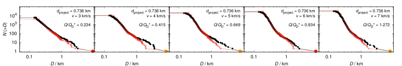
Figure 5: SFDs constructed from five different simulations with $D_{\rm pb}=10\,\rm km$, $d_{\rm project}=0.736\,\rm km$ and impact angle $\phi_{\rm imp}=45^{\circ}$. Black histogram shows the runs with the nonuniform distribution generated by the method of Diehl et al. (2012), while red are the previous (lattice) results shown in Fig. 10.

Appendix B Energy conservation vs. timestepping

Figure 6: Relative total energy $E$ vs time $t$ for the same grid of simulations as presented in Sec. 3. The diameter of the target was always $D=10\,{\rm km}$ and the impact angle $\phi_{\rm imp}=45^{\circ}$. The maximum relative energy error is of the order of $10^{-2}$ at the final time $t=10\,{\rm s}$.

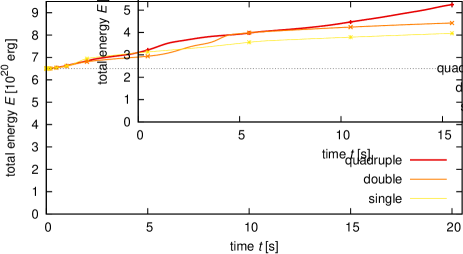
Figure 7: Total energy $E$ vs time $t$ for a small cratering impact, with a $D=1\,{\rm km}$ target and $d=22\,{\rm m}$ projectile, and several compiled numerical precisions of the SPH5 code: quadruple (128-bit), double (64-bit) and single (32-bit). Because the computation in quadruple precision is very slow, we use $N\doteq 1.4\times 10^{4}$ particles only in this test. Other parameters were set up similarly as in other simulations presented in Sec. 3. Neither version conserves the energy sufficiently, which is an indication that round-off errors are not the dominant cause of the energy increase.

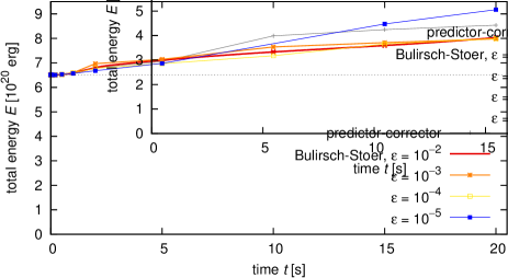
Figure 8: Total energy $E$ vs time $t$ for the same impact as in Fig. 8, but with different timestepping schemes, namely the default predictor–corrector (controlled by the Courant number $C=1.0$ and other time step restrictions) and the Bulirch–Stoer with the unitless parameter $\epsilon_{\rm BS}=10^{-2}$ to $10^{-5}$. The scaling by maximum values of variables was used, which corresponds to constant absolute errors. The energy conservation was somewhat improved this way, with the exception of the lowest $\epsilon_{\rm BS}$ at late times.

Modelling of smaller breakups seems more difficult. Apart from poor resolution of the impactor, if one uses the same (optimum) SPH particle mass as in the target, and a relatively low number of ejected fragments, weak impacts may also exhibit problems with energy conservation (see Fig. 6). This is even more pronounced in the case of low-speed collisions, e.g. of $D=1\,{\rm km}$ target, $d=22\,{\rm m}$ projectile, at $v_{\rm imp}=3\,{\rm km}/{\rm s}$ and $\phi_{\rm imp}=45^{\circ}$.

At first, we thought that small oscillations of density — with relative changes $\Delta\rho/\rho$ smaller than the numerical precision — are poorly resolved, and subsequently cause the total energy to increase. But when we performed the same simulation in quadruple precision (with approximately 32 valid digits) we realised there is essentially no improvement (see Fig. 7), so this cannot be the true reason.

Instead, we changed the timestepping scheme and superseded the default predictor/corrector with the Bulirsch–Stoer integrator (Press et al., 1992), which performs a series of trial steps with $\Delta t$ divided by factors $2,4,6,\dots$, and checks if the relative difference between successive divisions is less than small dimensionless factor $\epsilon_{\rm BS}$ and then extrapolates to $\Delta t\to 0$. In our case, a scaling of quantities is crucial. In principle, we have three options: (i) scaling by expected maximum values, which results in a constant absolute error; (ii) current values, or constant relative error; (iii) derivatives times time step, a.k.a. constant cumulative error. The option (i) seems the only viable one, otherwise the integrator is exceedingly slow during the initial pressure build-up. According to Fig. 8, we have managed to somewhat improve the energy conservation this way, but more work is needed to resolve this issue.

Appendix C Energy conservation vs sub-resolution acoustic waves

Even though we always start with intact monolithic targets, we realized that prolonged computations of the fragmentation phase require a more careful treatment of undamaged/damaged boundaries. The reason is the following rather complicated mechanism: (i) The shock wave, followed by a decompression wave, partially destroys the target. After the reflection from the free surface, the rarefaction (or sound) wave propagates back to the target. (ii) However, neither wave can propagate into already damaged parts, so there is only an undamaged cavity. (iii) This cavity has an irregular boundary, so that reflections from it create a lot of small waves, interfering with each other. (iv) As a result of this interference, there is a lot of particles that have either high positive or high negative pressure, so that the pressure gradient — computed as a sum over neighbours — is zero! (v) $\nabla P=0$ means no motion, and consequently no pressure release is possible. (vi) However, at the boundary between undamaged/damaged material, there are some particles with $P>0$, next to the damaged ones with $P=0$, which slowly push away the undamaged particles in the surroundings. (vii) Because the pressure is still not released, the steady pushing eventually destroys the whole target (see Fig. 9).

In reality, this does not happen, because the waves can indeed become very small and dissipate. In SPH, the dissipation of waves at the resolution limit is impossible. Increasing resolution does not help at all — the boundary is even more irregular and the sound waves will anyway become as small as the resolution.

As a solution, we can use an upper limit for damage, very close to 1, but not equal to 1, e.g. $(1-{\cal D})=10^{-12}$. Then the acoustic waves are damped (in a few seconds for $D=1\,{\rm km}$ targets) and the energy is conserved perfectly. Another option would be to use a more detailed rheology of the material, namely the internal friction and Drucker–Prager yield criterion (as in Jutzi et al., 2015).

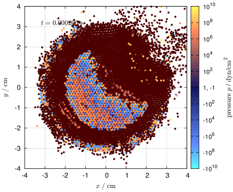
Figure 9: A simulation of the classical Nakamura (1993) experiment, but prolonged up to $200\,\mu{\rm s}$, which exhibits problems with energy conservation, as explained in the main text. We show a cross section in the $(x,y)$ plane and pressure $P$ in colour logarithmic scale. There are acoustic waves with wavelengths close to the resolution limit in the inner monolithic cavity, surrounded by fully damaged material (with ${\cal D}=1$). In our setup, $D_{\rm target}=6\,{\rm cm}$, $d_{\rm project}=0.7\,{\rm cm}$, $\rho=2.7$, or $1.15\,{\rm g}\,{\rm cm}^{-3}$ respectively, $v_{\rm imp}=3.2\,{\rm km}\,{\rm s}^{-1}$, $\phi_{\rm imp}=30^{\circ}$, $N_{\rm part}\doteq 7\cdot 10^{5}$.

Appendix D Additional figures

Figures D. 10 to D. 21 show the situation for non-standard impact angles.

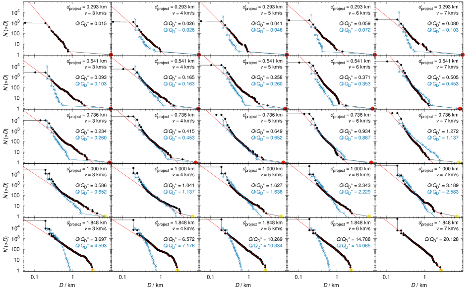
Figure 10: Impact angle 15^∘.

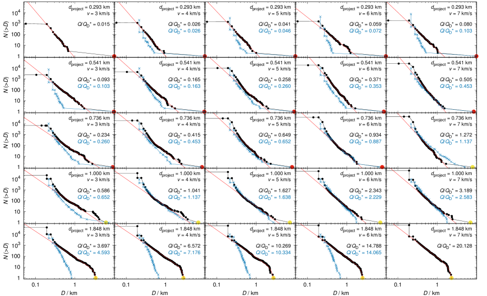
Figure 11: Impact angle 30^∘.

Figure 12: Impact angle 60^∘.

Figure 13: Impact angle 75^∘.

Figure 14: Impact angle 15^∘.

Figure 15: Impact angle 30^∘.

Figure 16: Impact angle 60^∘.

Figure 17: Impact angle 75^∘.

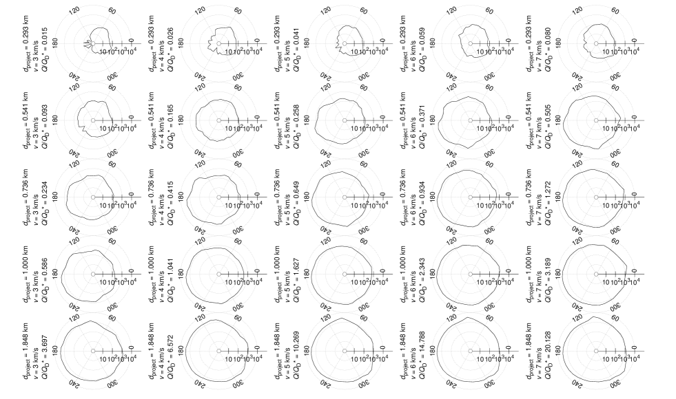
Figure 18: Impact angle 15^∘.

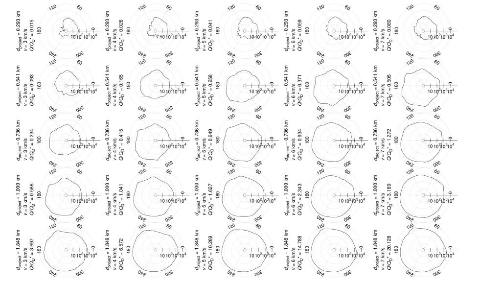
Figure 19: Impact angle 30^∘.

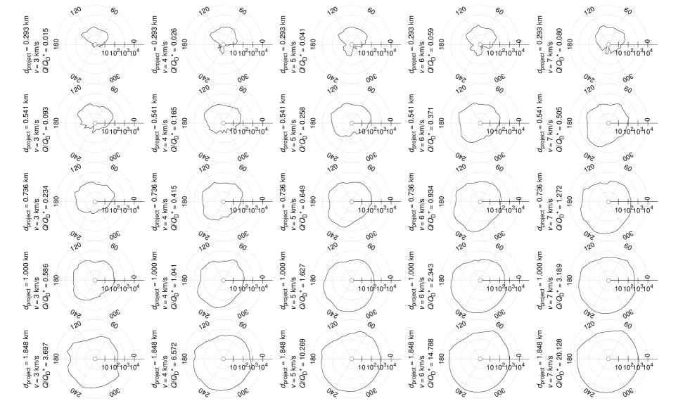
Figure 20: Impact angle 60^∘.

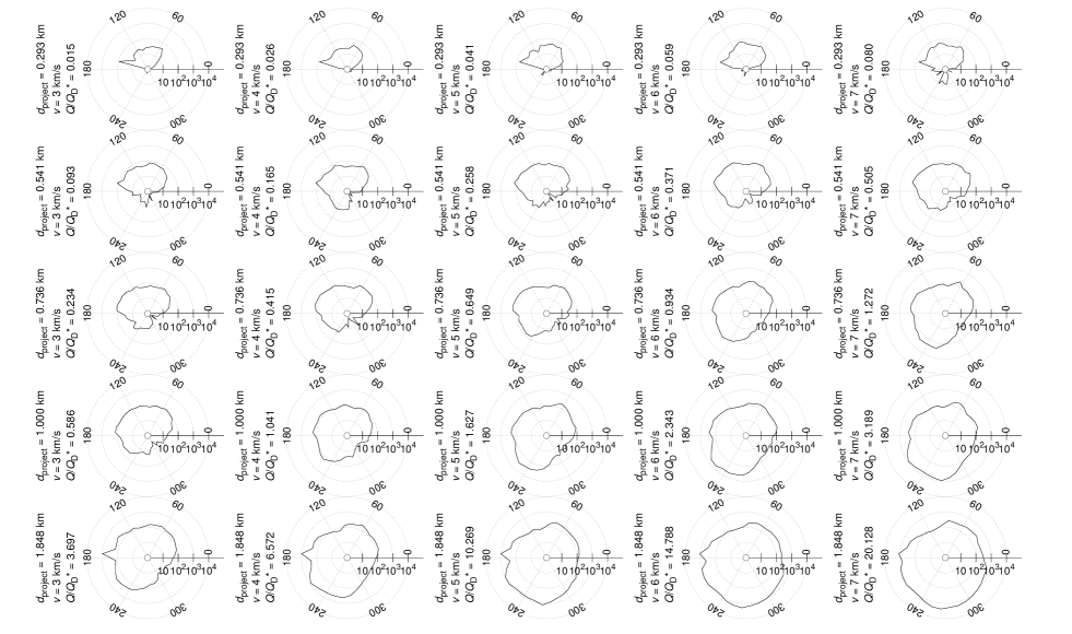
Figure 21: Impact angle 75^∘.

References

- Asphaug et al. (2015) Asphaug, E., Collins, G., Jutzi, M., 2015. Global scale impacts. Asteroids IV, 661–677.
- Benavidez et al. (2012) Benavidez, P. G., Durda, D. D., Enke, B. L., Bottke, W. F., Nesvorný, D., Richardson, D. C., Asphaug, E., Merline, W. J., May 2012. A comparison between rubble-pile and monolithic targets in impact simulations: Application to asteroid satellites and family size distributions. Icarus 219, 57–76.
- Benz and Asphaug (1994) Benz, W., Asphaug, E., Jan. 1994. Impact simulations with fracture. I - Method and tests. Icarus 107, 98.
- Benz and Asphaug (1999) Benz, W., Asphaug, E., Nov. 1999. Catastrophic Disruptions Revisited. Icarus 142, 5–20.
- Cibulková et al. (2014) Cibulková, H., Brož, M., Benavidez, P. G., Oct. 2014. A six-part collisional model of the main asteroid belt. Icarus 241, 358–372.
- Cossins (2010) Cossins, P. J., Jul. 2010. The Gravitational Instability and its Role in the Evolution of Protostellar and Protoplanetary Discs. Ph.D. thesis, University of Leicester.
- Davis and Ryan (1990) Davis, D. R., Ryan, E. V., 1990. On collisional disruption: Experimental results and scaling laws. Icarus 83 (1), 156 – 182.
- Diehl et al. (2012) Diehl, S., Rockefeller, G., Fryer, C. L., Riethmiller, D., Statler, T. S., Nov. 2012. Generating Optimal Initial Conditions for Smooth Particle Hydrodynamics Simulations. ArXiv e-prints.
- Durda et al. (2007) Durda, D. D., Bottke, W. F., Nesvorný, D., Enke, B. L., Merline, W. J., Asphaug, E., Richardson, D. C., Feb. 2007. Size-frequency distributions of fragments from SPH/N-body simulations of asteroid impacts: Comparison with observed asteroid families. Icarus 186, 498–516.
- Grady and Kipp (1980) Grady, D., Kipp, M., 1980. Continuum modelling of explosive fracture in oil shale. International Journal of Rock Mechanics and Mining Sciences & Geomechanics Abstracts 17 (3), 147 – 157.
- Herant (1994) Herant, M., 1994. Dirty Tricks for SPH (Invited paper) 65, 1013.
- Herrmann (1969) Herrmann, W., 1969. Constitutive equation for the dynamic compaction of ductile porous materials. Journal of Applied Physics 40 (6), 2490–2499.
- Hirayama (1918) Hirayama, K., Oct. 1918. Groups of asteroids probably of common origin. AJ31, 185–188.
- Jutzi et al. (2015) Jutzi, M., Holsapple, K., Wünneman, K., Michel, P., Feb. 2015. Modeling asteroid collisions and impact processes. Asteroids IV.
- Leinhardt and Stewart (2012) Leinhardt, Z. M., Stewart, S. T., Jan. 2012. Collisions between Gravity-dominated Bodies. I. Outcome Regimes and Scaling Laws. Astrophys. J. 745, 79.
- Michel et al. (2001) Michel, P., Benz, W., Paolo, T., Richardson, D. C., 2001. Collisions and gravitational reaccumulation: Forming asteroid families and satellites. Science 294 (5547), 1696–1700.
- Michel et al. (2003) Michel, P., Benz, W., Richardson, D. C., Feb. 2003. Disruption of fragmented parent bodies as the origin of asteroid families. Nature 421, 608–611.
- Michel et al. (2004) Michel, P., Benz, W., Richardson, D. C., Apr. 2004. Catastrophic disruption of pre-shattered parent bodies. Icarus 168, 420–432.
- Michel et al. (2011) Michel, P., Jutzi, M., Richardson, D. C., Benz, W., Jan. 2011. The Asteroid Veritas: An intruder in a family named after it? Icarus 211, 535–545.
- Michel et al. (2002) Michel, P., Tanga, P., Benz, W., Richardson, D. C., 2002. Formation of asteroid families by catastrophic disruption: Simulations with fragmentation and gravitational reaccumulation. Icarus 160 (1), 10 – 23.
- Monaghan and Gingold (1983) Monaghan, J., Gingold, R., 1983. Shock simulation by the particle method sph. Journal of Computational Physics 52 (2), 374 – 389.
- Morbidelli et al. (2009) Morbidelli, A., Bottke, W. F., Nesvorný, D., Levison, H. F., Dec. 2009. Asteroids were born big. Icarus 204, 558–573.
- Nakamura and Fujiwara (1991) Nakamura, A., Fujiwara, A., Jul. 1991. Velocity distribution of fragments formed in a simulated collisional disruption. Icarus 92, 132–146.
- Nesvorný et al. (2015) Nesvorný, D., Brož, M., Carruba, V., Feb. 2015. Identification and Dynamical Properties of Asteroid Families. Asteroids IV.
- Nesvorný et al. (2006) Nesvorný, D., Enke, B. L., Bottke, W. F., Durda, D. D., Asphaug, E., Richardson, D. C., Aug. 2006. Karin cluster formation by asteroid impact. Icarus 183, 296–311.
- Press et al. (1992) Press, W. H., Teukolsky, S. A., Vetterling, W. T., Flannery, B. P., 1992. Numerical recipes in FORTRAN. The art of scientific computing.
- Price (2008) Price, D. J., Dec. 2008. Modelling discontinuities and Kelvin Helmholtz instabilities in SPH. Journal of Computational Physics 227, 10040–10057.
- Price (2012) Price, D. J., Feb. 2012. Smoothed particle hydrodynamics and magnetohydrodynamics. Journal of Computational Physics 231, 759–794.
- Richardson et al. (2000) Richardson, D. C., Quinn, T., Stadel, J., Lake, G., Jan. 2000. Direct Large-Scale N-Body Simulations of Planetesimal Dynamics. Icarus 143, 45–59.
- Rosswog (2009) Rosswog, S., Apr. 2009. Astrophysical smooth particle hydrodynamics. New A Rev.53, 78–104.
- Rosswog (2015) Rosswog, S., Apr. 2015. Boosting the accuracy of SPH techniques: Newtonian and special-relativistic tests. Mon. Not. R. Astron. Soc. 448, 3628–3664.
- Tillotson (1962) Tillotson, J. H., Jul. 1962. Metallic equations of state for hypervelocity impact. General Atomic Report GA-3216.
- von Mises (1913) von Mises, R., 1913. Mechanik der festen körper im plastisch- deformablen zustand. Nachrichten von der Gesellschaft der Wissenschaften zu Göttingen, Mathematisch-Physikalische Klasse 1913, 582–592.
- Weibull (1939) Weibull, W., 1939. A Statistical Theory of the Strength of Materials. Ingeniörsvetenskapsakademiens handlingar. Generalstabens litografiska anstalts förlag.