Asymptotic behavior of the velocity distribution of driven inelastic gas with scalar velocities: analytical results

Abstract

We determine the asymptotic behavior of the tails of the steady state velocity distribution of a homogeneously driven granular gas comprising of particles having a scalar velocity. A pair of particles undergo binary inelastic collisions at a rate that is proportional to a power of their relative velocity. At constant rate, each particle is driven by multiplying its velocity by a factor $-r_{w}$ and adding a stochastic noise. When $r_{w}<1$, we show analytically that the tails of the velocity distribution are primarily determined by the noise statistics, and determine analytically all the parameters characterizing the velocity distribution in terms of the parameters characterizing the stochastic noise. Surprisingly, we find logarithmic corrections to the leading stretched exponential behavior. When $r_{w}=1$, we show that for a range of distributions of the noise, inter-particle collisions lead to a universal tail for the velocity distribution.

1 Introduction

Granular systems are ubiquitous in nature. Examples include sand, powders, grains, interstellar objects like asteroids and so on. Composed of macroscopic particles, the combination of inelastic collisions and external driving results in granular systems exhibiting complex phenomena such as size segregation, pattern formation, jamming, memory effects, shocks, etc. Jaeger:96 ; Aranson:06 ; Goldhirsch:93 ; Li:03 ; Corwin:05 ; Prados:14 ; Lasanta:17 ; joy2017shock . Being far from equilibrium, a general theory to understand granular systems has been lacking. However, a class of systems for which theoretical progress has been possible are dilute granular matter, also known as granular gases. In addition to exhibiting complex macroscopic behavior, granular gases have been a testing ground for both kinetic theory as well as for simple solvable models.

When isolated, a portion of the kinetic energy of the granular gas is dissipated in each collision, and the constituent particles eventually form clusters leading to strong spatial inhomogeneities Goldhirsch:93 ; Brey:96 ; Esipov:97 ; Ben-naim:99 ; Ben-naim:00 ; Nie:02 ; Supravat:11 ; Pathak:14a ; Pathak:14 ; shinde2007violation ; Subhajit:14 ; Subhajit:17 ; brilliantov2018increasing . However, when driven homogeneously the system reaches a steady state that is homogeneous in space Vanzon:04 ; Scholz:17 . The single particle velocity distribution $P(v)$ [‘$v$’ is the magnitude of the velocity which is in general a vector] of such driven granular gases has been the subject of many different studies. Of particular interest is the question of whether the asymptotic behaviour of $P(v)$ is universal, and if yes then what its form is. This question has been addressed in several experiments, numerical simulations, and within kinetic theory. A recent review may be found in Ref. windows2017granular . Experimental systems of driven granular gases typically consists of collections of granular particles, such as steel, glass beads, etc., that may be spherical, ellipsoidal, dumbbell-shaped, etc., that undergo inelastic collisions and is driven either through collision of the particles with vibrating walls Clement:91 ; Warr:95 ; Kudrolli:97 ; Olafsen:98 ; Olafsen:99 ; Losert:99 ; Kudrolli:00 ; Rouyer:00 ; Blair:01 ; Vanzonexpt:04 ; reis2007forcing ; wang2009particle ; Scholz:17 ; vilquin2018shock ; wildman2009granular or as bilayers where the vibrated bottom layer drives the top layer Baxter:03 ; baxter2007temperature ; windows2013boltzmann , or by using electric Aranson:02 ; Kohlstedt:05 or magnetic fields Schmick:08 ; Falcon:2013 . In some experiments, the effects of gravity are minimised by performing them in microgravity tatsumi2009experimental ; hou2008velocity ; grasselli2015translational . Several experiments observe a universal stretched exponential form $P(v)\sim\exp(-a|v|^{\beta})$ with $\beta\approx 1.5$ for wide range of system parameters Losert:99 ; Rouyer:00 ; Aranson:02 ; reis2007forcing ; wang2009particle ; tatsumi2009experimental ; Scholz:17 ; vilquin2018shock , while other experiments find that $\beta$ differs from $1.5$ and lies between $1$ and $2$ or is a gaussian, and may depend on the driving parameters Olafsen:99 ; Kudrolli:00 ; Blair:01 ; baxter2007temperature ; Schmick:08 ; hou2008velocity ; wildman2009granular ; Falcon:2013 ; windows2013boltzmann ; grasselli2015translational . Numerical simulations puglisi1998clustering ; puglisi1999kinetic ; Moon:01 ; Vanzon:04 ; Vanzon:05 ; Cafiero:2002 ; burdeau2009quasi ; gayen2008orientational ; gayen2011effect ; rui2011velocity ; Prosendas:18 ; kang2010granular have also been inconclusive. The velocity distribution for a one dimensional gas driven through a thermal bath is observed to have a gaussian form in the quasi-elastic limit but deviates from gaussian when the collisions are inelastic puglisi1998clustering ; puglisi1999kinetic . For a three dimensional granular gas driven homogeneously with a momentum conserving noise, it was shown that $\beta\approx 1.5$ for large inelasticity, whereas $\beta$ approaches $2$ when collisions are near-elastic Moon:01 . Also, when the granular gas is polydispersed, one finds a range of $\beta$ rui2011velocity . Similar study on a bounded two dimensional granular system observes $\beta\approx 2$ for a range of coefficient of restitution and density Vanzon:04 ; Vanzon:05 , while a two dimensional system driven through the rotational degrees of freedom find $\beta\approx 1.42$ Cafiero:2002 . Molecular dynamics simulations of a uniformly heated granular gas with solid friction find $\beta=2$ Prosendas:18 . Sheared granular gases have also been studied via simulations, which find $\beta\approx 1.5$ gayen2008orientational ; gayen2011effect , while those for bilayers show $\beta=2$ burdeau2009quasi . Models with extremal driving have also been studied which exhibit intermediate power law behaviour kang2010granular . Finding the asymptotic behavior of the velocity statistics from experiments and direct simulations is challenging due to poor sampling near the tails and the presence of strong crossovers from the behaviour of the distribution at small velocities to the asymptotic behaviour at high velocities, making it difficult to unambiguously determine $\beta$.

In the homogeneous limit, the analysis may be simplified by integrating out or ignoring the spatial degrees of freedom. The velocity distribution may then be studied either using kinetic theory Brilliantov:04 where molecular chaos is assumed to break BBGKY hierarchy, or by analyzing simple microscopic models like the inelastic Maxwell model Bobylev:00 ; Ben-naim:00 , where the collision rate between particles is assumed to be the same for all pairs of particles. Within kinetic theory, the tail of the velocity distribution may be determined by linearizing the Boltzmann equation Noije:98 . When the rate of collision of a pair of particles is proportional to their relative velocities and the driving is described by a diffusive term, it was shown that the velocity distribution for large velocities $|v|\gg v_{rms}$, is a stretched exponential with exponent $\beta=3/2$ Noije:98 , independent of spatial dimension. In Maxwell gases, most of the rigorous results are for systems with scalar (one dimensional) velocities, as the collisions in 2 and 3 dimensions are more complicated. Maxwell gases with scalar velocities, with constant rate of collision and diffusive driving ($d{v}/dt={\eta}$ where ${\eta}$ is gaussian white noise), may be solved exactly to yield an exponential decay for the velocity distribution with $\beta=1$ Ernst:02 ; Antal:02 ; Santos:03 . Both these cases can be analysed using single framework by considering a general model where a pair of particles with relative velocity $\vec{v}$ collide with rate $|\vec{v}|^{\delta}$ Ernst2003 ; ernst2006rich ; ernst2006 ; barrat2007quasi . Even though one is especially interested in physical limit of $\delta=1$ (also called hard-spheres), the general model is useful for more general kernels which may phenomenologically have other values of $\delta$ Kohlstedt:05 . Note also, that in elastic kinetic theory $\delta=-3$ corresponds to Coulomb interaction. For the model with collision rate $|\vec{v}|^{\delta}$ the Boltzmann equation with diffusive driving may be analyzed to yield $\beta=(2+\delta)/2$ Ernst2003 retrieving the special limits of hardsphere ($\delta=1$) and Maxwell ($\delta=1$) gases. For a review on results obtained from kinetic theory, see Ref. Villani:06 .

Within the molecular chaos hypothesis, the main issue is how to model noise. While the tails may be determined for random acceleration (diffusive driving) the system does not reach a steady state, as the velocity of the center of mass does a random walk leading to the linear divergence of total energy with time Prasad:13 . Hence the steady state solutions for diffusive driving is valid only on the center of mass frame. A more realistic driving scheme is dissipative driving, in which when a particle with velocity $\vec{v}$ is driven, its velocity is modified to $\vec{v}^{\prime}=-r_{w}\vec{v}+{{\bf\eta}}$, where $\vec{v}^{\prime}$ is the new velocity, $r_{w}$ is a parameter by which the velocity is dissipated and ${\bf{\eta}}$ is uncorrelated random noise taken from a distribution $\Phi({\bf{\eta}})$ Prasad:13 . For $r_{w}\in(-1,1]$, the system reaches a steady state at long times Prasad:13 . The model with scalar velocities and dissipative driving has been recently studied in detail Prasad:17 for noise distributions that has the asymptotic behavior $\Phi(\eta)\sim\exp(-b|\eta|^{\gamma})$ for $\eta^{2}\gg\langle\eta^{2}\rangle_{\Phi}$, where the average $\langle..\rangle_{\Phi}$ refers to averaging over the noise distribution $\Phi(\eta)$. By studying the moment equations numerically Prasad:17 , it was shown that when $r_{w}<1$, the velocity distribution $P(v)\sim\exp(-a|v|^{\beta})$, is non-universal with $\beta=\gamma$, while when $r_{w}=1$, $\beta=\min(\gamma,1)$. Thus, $\beta$ is universal (independent of noise) only when $r_{w}=1$ and $\gamma\geq 1$. One could also make predictions about the coefficient $a$. It was observed numerically that $a=b$ for $\gamma<1$ and $a\neq b$ for $\gamma>1$. All these results were based on numerical analysis and restricted to the case $\delta=0$, corresponding to the Maxwell gas. The exact form of $a$ is known for the Maxwell gas only for two cases: one, for $r_{w}<1$ and $\gamma=2$ when $a=b(1-r_{w}^{2})$ Prasad:13 , and other, for $r_{w}=1$ and $\gamma\geq 1$, when $a=\omega^{*}$, where $\omega^{*}$ is the solution for $1=\lambda_{d}f(\omega)$, with $\lambda_{d}$, the rate of driving and $f(\omega)=\langle e^{-i\omega\eta}\rangle_{\Phi}$, the characteristic function of the noise distribution Prasad:17 . We note that, for both diffusive driving as well as dissipative driving, all exact results have been limited to the case $\delta=0$.

In this paper, we choose to study a system with scalar velocities as the analysis there is much simpler (Study of an inelastic gas with two-dimensional velocities may be found in Ref. Prasad:19 ). For the inelastic gas with scalar velocities, driven homogeneously through dissipative driving, we carry out an exact analysis of the equations satisfied by the moments of the velocity for a general collision kernel, corresponding to arbitrary $\delta$. To our knowledge, this is the only solution that exists for non-zero $\delta$. We determine the different parameters of the velocity distribution in terms of the asymptotic behavior of the noise distribution $\Phi(\eta)$ that is characterized by the parameters $\gamma$, $b$, and ${\tilde{\chi}}$ through $\Phi(\eta)\sim|\eta|^{\tilde{\chi}}\exp(-b|\eta|^{\gamma})$ for large $|\eta|$. Surprisingly, we find the presence of logarithmic corrections to the leading stretched exponential decay even in the absence of any such corrections in $\Phi(\eta)$. In addition, the distribution depends strongly on whether $|r_{w}|<1$ or $r_{w}=1$. In particular, for large velocities ($v^{2}\gg\langle v^{2}\rangle$), we assume that the leading behaviour for the velocity distribution is a stretched exponential. We show that, within this assumption, a self-consistent solution for the equations satisfied by the moments of the velocity may be found. Though we are unable to show the uniqueness of our self-consistent solution, we believe that the results, thus obtained, are exact. Our results are summarised below. We show that asymptotically, the velocity distribution decays as

$$\ln P(v)=-a|v|^{\beta}-a^{\prime}(\ln|v|)^{2}+\chi\ln|v|+\ldots,~{}~{}|r_{w}|<1,$$ (1)

where

$$\begin{split}\beta=&\gamma,\\ a=&\begin{cases}b,\qquad\qquad\qquad\quad\gamma\leq 1,\\ b\left[1-r_{w}^{\frac{\gamma}{\gamma-1}}\right]^{\gamma-1},~{}\gamma>1,\\ \end{cases}\\ a^{\prime}=&\begin{cases}0,\qquad\qquad\qquad\qquad~{}~{}\gamma\leq 1,\\ \frac{\gamma(\gamma-1)}{2\ln(r_{w})}\left[\frac{1}{\gamma}+\frac{\tilde{\chi}}{\gamma}-\frac{\tilde{\delta}}{\gamma}-\frac{1}{2}\right],~{}\gamma>1,\\ \end{cases}\\ \chi=&\begin{cases}\tilde{\chi}-\tilde{\delta},~{}~{}\gamma\leq 1,\\ 0,~{}~{}~{}~{}~{}~{}~{}~{}~{}\gamma>1\end{cases}\end{split}$$ (2)

where $\tilde{\delta}=\max[\delta,0]$. For $r_{w}=1$, we show that when $\delta\leq 0$,

$$\ln P(v)=-a|v|^{\beta}+\ldots,~{}~{}r_{w}=1,~{}-2<\delta\leq 0,$$ (3)

where

$$\beta= \min\left[\frac{2+\delta}{2},\gamma\right],\quad r_{w}=1,~{}-2<\delta\leq 0,$$ (4)

$$a= \begin{cases}\frac{4}{2+\delta}\sqrt{\frac{\lambda_{d}}{N_{2}\lambda_{c}}},~{}-2<\delta<0,~{}~{}\frac{2+\delta}{2}<\gamma,\\ \omega^{*},\qquad\qquad~{}~{}~{}~{}~{}\delta=0,\qquad~{}~{}~{}~{}1\leq\gamma,\\ b,\qquad\qquad\quad~{}~{}~{}~{}\delta\leq 0,\qquad~{}\frac{2+\delta}{2}>\gamma,\end{cases}$$ (5)

where $N_{2}$ is the second moment of the noise distribution, and $\lambda_{c}$ and $\lambda_{d}$ are rates for collision and driving respectively [see Sec. 2 for a precise definition of rates], and $\omega^{*}$ is the solution for $1=\lambda_{d}f(\omega)$, with $f(\omega)=\langle e^{-i\omega\eta}\rangle_{\Phi}$ being the characteristic function of the noise distribution Prasad:17 . For $r_{w}=1$ and $\delta>0$, we show that

$$\ln P(v)=-a|v|(\ln|v|)^{\frac{\gamma-1}{\gamma}}+\ldots,r_{w}=1,\delta>0,\gamma>1,$$ (6)

where

$$a=\left[\left(\frac{\delta\gamma}{\gamma-1}\right)^{\gamma-1}b\gamma\right]^{\frac{1}{\gamma}},r_{w}=1,\delta>0,\gamma>1.$$ (7)

When $\gamma\leq 1$ and $\delta>0$, the velocity distribution is asymptotically same as that of the noise distribution.

The remainder of the paper is organized as follows. In Sec. 2, we define the model precisely. Section 3 contains a detailed analysis of the equation satisfied by the various moments of the velocity distribution. This analysis allows us to obtain a precise characterization of the asymptotic behavior of the distribution. The analytical results for $\delta=0$, thus obtained, are compared with results from numerical analysis in Sec. 4. Section. 5 contains a summary and discussion of the results.

2 Model

Consider $N$ particles, labeled $i=1,\ldots,N$, of equal mass, each having a scalar velocity denoted by $v_{i}$. The velocities evolve through both momentum-conserving inelastic collisions among particles as well as external driving. Particles $i$ and $j$ collide at a rate $2\lambda_{c}|v_{i}-v_{j}|^{\delta}/(N-1)$. The factor $2/(N-1)$ is included so that the total rate of collision of the $N(N-1)/2$ pairs is proportional to $N$. For Maxwell gases the collision rate is independent of the relative velocity, i.e., $\delta=0$, while for hard sphere gases the collision rate is proportional to the relative velocity, i.e., $\delta=1$. In a collision, momentum is conserved and the velocities are modified according to

$$\begin{split}v_{i}^{\prime}&=(1-\alpha)v_{i}+\alpha v_{j},\\ v_{j}^{\prime}&=\alpha v_{i}+(1-\alpha)v_{j},\end{split}$$ (8)

where the unprimed and primed ($\prime$) velocities refers to the pre- and post-collision velocities. Also,

$$\alpha=\frac{1+r}{2},$$ (9)

where $r\in[0,1)$ is the coefficient of restitution, such that $\alpha\in[1/2,1)$. The two limits $r=1$ ($\alpha=1$) and $r=0$ ($\alpha=1/2$) correspond to elastic and maximally dissipative collisions respectively.

Each particle is driven at rate $\lambda_{d}$. When driven, the new velocity of a particle is given by

$$v_{i}^{\prime}=-r_{w}v_{i}+\eta,$$ (10)

where $r_{w}\in(-1,1]$ quantifies how the speed is reduced upon driving, and the noise $\eta$ mimics stochasticity in driving. Though this form of driving was introduced earlier Prasad:13 , we give below several motivations to chose this particular model of driving.

Firstly, when $r_{w}\not=-1$ [Eq. (10)] the system reaches a steady state at large times, and overcomes the drawback of diffusive driving ($r_{w}=-1$) for which there is no steady state. For the Maxwell gas, this may be shown analytically by obtaining the exact time evolution of the total energy Prasad:13 . For a general collision kernel, the existence of steady state may be seen through Monte Carlo simulations for both the gas with one-dimensional velocities Prasad:13 , as well as two-dimensional velocities Prasad:19 . Secondly, the driving in the limit $r_{w}=1$ captures the scenario described by kinetic theory models with a diffusive term for driving, and thus provides a rigorous check for its predictions of $\beta=3/2$. To understand this, let us examine the evolution of the distribution function $P(v,t)$:

$$\frac{dP(v,t)}{dt}= -2\lambda_{c}\int dv_{2}|v-v_{2}|^{\delta}P(v,t)P(v_{2},t)$$

$$+2\lambda_{c}\int\int dv_{1}dv_{2}|v_{1}-v_{2}|^{\delta}P(v_{1},t)P(v_{2},t)\delta\left[(1-\alpha)v_{1}+\alpha v_{2}-v\right]$$

$$-\lambda_{d}P(v,t)+\lambda_{d}\int\int d\eta dv_{1}\Phi(\eta)P(v_{1},t)\delta\left[-r_{w}v_{1}+\eta-v\right],$$ (11)

where the the product measure for the joint distribution $P(v_{1},v_{2})=P(v_{1})P(v_{2})$ is invoked, due to lack of correlations between the velocities of different particles in the large system size limit, arising from the fact that pairs of particles collide at random. Note that this is true only in the steady state and that for diffusive driving, the system does not reach a steady state due to diverging correlations between particles Prasad:13 . The first two terms on the right hand side of Eq. (11) describe the loss and gain terms due to inter-particle collisions. The third and fourth terms on the right hand side describe the loss and gain terms due to driving. The driving terms may be analysed for small $\eta$ as follows. Let

$$I_{D}=-\lambda_{d}P(v,t)+\lambda_{d}\int\int d{\eta}dv_{1}\Phi(\eta)P(v_{1},t)\frac{1}{r_{w}}\delta\left[\frac{\eta-v}{r_{w}}-v_{1}\right].$$ (12)

Integrating over $v_{1}$, and using the symmetry of the distribution $P(v)=P(-v)$, we obtain

$$I_{D}=-\lambda_{d}P(v,t)+\frac{\lambda_{d}}{r_{w}}\int\int d\eta dv\Phi(\eta)P\left(\frac{v-\eta}{r_{w}},t\right).$$ (13)

Now setting $r_{w}=1$, and Taylor expanding the integrand about $\eta=0$, and then integrating over $\eta$, Eq. (13) reduces to

$$I_{D}=\frac{\lambda_{d}\langle\eta^{2}\rangle}{2}\frac{\partial^{2}P(v)}{\partial v^{2}}+\mathrm{higher~{}order~{}terms},\quad r_{w}=1.$$ (14)

When the higher order terms are ignored, the resulting equation for $P(v)$ for $r_{w}=1$ is the same as that was analysed in Ref. Noije:98 to obtain the well-known result of $\ln P(v)\sim-v^{3/2}$. It is not apriori clear whether this truncation is valid. This is because the tails of the velocity distribution could be affected by tails of the noise distribution, in which case higher order moments of noise may contribute.

Thirdly, the model of dissipative driving may also be motivated by experimental systems, where driving is usually through collisions with a massive wall. In such a wall-particle collision event, the velocity of a particle $i$, $v_{i}$ and that of the wall, $v_{w}$ change to $v_{i}^{\prime}$ and $v_{w}^{\prime}$ respectively according to $(v_{i}^{\prime}-v_{w}^{\prime})=-r_{w}(v_{i}-v_{w})$, where $r_{w}$ is the coefficient of restitution for the wall-particle collision. Considering $v_{w}^{\prime}\approx v_{w}$, for a massive wall, rearranging and replacing $(1+r_{w})v_{w}$ by a noise $\eta$ results in Eq. (10). Within this motivation, $r_{w}$ takes only positive values. Since the stochasticity does not arise from a sum of many events, there is no compelling reason for the distribution for noise $\Phi(\eta)$ to be a gaussian. For example, in experiments with sinusoidally oscillating wall driving the particles, if the collision times are assumed to be random, $\Phi(\eta)\sim(c^{2}-\eta^{2})^{-1/2}$, with $\eta\in(-c,c)$ Prasad:19 . This corresponds to the asymptotic behaviour of the noise being $\Phi(\eta)\sim\exp(-a|\eta|^{\gamma})$ with $\gamma=\infty$. To incorporate the general case where the tails of the noise distribution may differ from a gaussian, we could consider noise distributions which decay either as a stretched exponential or as a power law or faster than a stretched exponential (for example $\exp[-e^{|\eta|}]$). However, we find that the power law tail and distribution decaying faster than stretched exponential may be considered as special cases of the stretched exponential form [$\gamma=0$ and $\gamma=\infty$ respectively in Eq. (15)] for large values of $\eta$. For these reasons, we consider a set of noise distributions $\Phi(\eta)$ whose leading order asymptotic behaviour are stretched exponentials:

$$\ln\Phi(\eta)\sim-b|\eta|^{\gamma}+\ldots+\tilde{\chi}\ln|\eta|,~{}b,\gamma>0,~{}\mathrm{for~{}}\eta^{2}\gg\langle\eta^{2}\rangle_{\Phi},$$ (15)

where $\langle\cdots\rangle_{\Phi}$ denotes average with respect to $\Phi(\eta)$.

3 Analysis of moments for arbitrary $\delta$

The equation obeyed by the different moments may be obtained by multiplying Eq. (11) by $v^{2n}$ and integrating over all velocities. In the steady state, after setting time derivatives to zero, we obtain

$$2\lambda_{c}[1-\alpha^{2n}-(1-\alpha)^{2n}]\langle|v-v_{1}|^{\delta}v^{2n}\rangle+\lambda_{d}(1-r_{w}^{2n})\langle v^{2n}\rangle=$$

$$2\lambda_{c}\sum_{k=1}^{2n-1}\binom{2n}{k}\alpha^{k}(1-\alpha)^{2n-k}\langle|v-v_{1}|^{\delta}v^{2n-k}v_{1}^{k}\rangle$$

$$+\lambda_{d}\sum_{k=1}^{n}\binom{2n}{2k}r_{w}^{2n-2k}\langle v^{2n-2k}\rangle N_{2k},~{}n=1,2,3,\ldots,$$ (16)

where $N_{2k}=\langle\eta^{2k}\rangle_{\Phi}$ is the $(2k)^{th}$ moment of the noise distribution, and $\langle\cdots\rangle$ denotes averaging with respect to the steady state velocity distribution. To clarify, in the case of joint moments such as $\langle|v-v_{1}|^{\delta}v^{2n-k}v_{1}^{k}\rangle$ and $\langle|v-v_{1}|^{\delta}v^{2n}\rangle$, the averaging needs to be performed over the joint probability distribution $P(v,v_{1})$.

We analyze Eq. (3) for large $n$. For large $n$, the left hand side of Eq. (3) is dominated by the first term when $\delta>0$, and by the second term when $\delta<0$. Also, since $1/2\leq\alpha<1$, the terms $\alpha^{2n}$ and $(1-\alpha)^{2n}$ are negligibly small, and we may rewrite Eq. (3) as

$$\langle|v-v_{1}|^{\tilde{\delta}}v^{2n}\rangle\sim\sum_{k=1}^{n}\binom{2n}{2k}r_{w}^{2n-2k}\langle v^{2n-2k}\rangle N_{2k}+$$

$$\sum_{k=1}^{2n-1}\binom{2n}{k}\alpha^{k}(1-\alpha)^{2n-k}\langle|v-v_{1}|^{\delta}v^{2n-k}v_{1}^{k}\rangle,~{}n\gg 1,$$ (17)

where

$$\tilde{\delta}=\begin{cases}\max(\delta,0),&r_{w}<1,\\ \delta,&r_{w}=1,\end{cases}$$ (18)

and $x\sim y$ means that $x/y=\mathcal{O}(1)$. The first and second terms on the right hand side of Eq. (3) arise due to driving and inter-particle collisions respectively.

We will assume that the velocity distribution is asymptotically a stretched exponential:

$$\ln P(v)=-a|v|^{\beta}+\Psi(|v|),~{}v^{2}\gg\langle v^{2}\rangle,$$ (19)

where $v^{-\beta}\Psi(v)\to 0$, when $v\gg 1$. The large moments may be computed using the saddle point approximation (see Appendix A) to give

$$\langle|v-v_{1}|^{\tilde{\delta}}v^{2n}\rangle\sim n^{\frac{1+\tilde{\delta}}{\beta}-\frac{1}{2}}\left[\frac{2n}{ae\beta}\right]^{\frac{2n}{\beta}}e^{\Psi\left[\left(\frac{2n}{a\beta}\right)^{\frac{1}{\beta}}\right]},$$ (20)

$$\langle|v-v_{1}|^{\delta}v^{2n-k}v_{1}^{k}\rangle\sim n^{\frac{2+\delta}{\beta}-1}\left[\frac{n}{ae\beta}\right]^{\frac{2n}{\beta}}\times$$ (21)

$$e^{n\left[\frac{2-x}{\beta}\ln(2-x)+\frac{x}{\beta}\ln(x)\right]}e^{\Psi\left[\left(\frac{(2-x)n}{a\beta}\right)^{\frac{1}{\beta}}\right]+\Psi\left[\left(\frac{xn}{a\beta}\right)^{\frac{1}{\beta}}\right]},$$

where $n\gg 1$ and where $x=k/n$, $k,n\gg 1$. A similar analysis shows that the moments of the noise distribution $\Phi(\eta)$ [as in Eq. (15)] has the asymptotic behavior

$$N_{2n}\sim n^{\frac{1+\tilde{\chi}}{\gamma}-\frac{1}{2}}\left[\frac{2n}{be\gamma}\right]^{\frac{2n}{\gamma}},~{}~{}n\gg 1.$$ (22)

The $(2n)^{th}$ moment of velocity diverges exponentially with $n$. Thus, each term in the right hand side of Eq. (3) is exponentially large, and the sums can be replaced by the largest term with negligible error. This largest term may belong to either the first or second sum. By keeping in Eq. (3) only the terms due to inter-particle collision, we obtain

$$\langle|v-v_{1}|^{\tilde{\delta}}v^{2n}\rangle\sim$$

$$\sum_{k=1}^{2n-1}\binom{2n}{k}\alpha^{k}(1-\alpha)^{2n-k}\langle|v-v_{1}|^{\delta}v^{2n-k}v_{1}^{k}\rangle,~{}n\gg 1,$$ (23)

whose self-consistent solution for $\beta$ will be denoted by $\beta_{c}$. Likewise, we denote by $\beta_{d}$ the self-consistent solution of $\beta$ for the equation obtained by dropping the collision term in Eq. (3):

$$\langle|v-v_{1}|^{\tilde{\delta}}v^{2n}\rangle\sim\sum_{k=1}^{n}\binom{2n}{2k}r_{w}^{2n-2k}\langle v^{2n-2k}\rangle N_{2k},~{}n\gg 1.$$ (24)

Clearly, the true solution for $\beta$ is

$$\beta=\min(\beta_{d},\beta_{c}).$$ (25)

We now determine $\beta_{c}$ and $\beta_{d}$.

3.1 Analysis of the collision term

We first analyze Eq. (3), that arises from keeping terms due to inter-particle collisions, and show that the only possible solution is $\beta_{c}=\infty$. Let $k=xn$, where $0\leq x\leq 2$. The summation on the right hand side of Eq. (3) may now be converted into an integral, $\sum_{k}\to n\int dx$. Approximating the factorials by the Stirling’s approximation, and on replacing the left hand side by using Eq. (20), Eq. (3) reduces to

$$\frac{n^{\frac{1+\tilde{\delta}}{\beta_{c}}}}{\sqrt{n}}\left[\frac{2n}{ae\beta_{c}}\right]^{\frac{2n}{\beta_{c}}}\sim\frac{n^{\frac{2+\delta+2\chi}{\beta_{c}}}}{\sqrt{n}}\left[\frac{n}{ae\beta_{c}}\right]^{\frac{2n}{\beta_{c}}}\int dxe^{nf(x)},$$ (26)

where we have also substituted the terms in the right hand side of Eq. (3) with the asymptotic form for the moments in Eq. (21). The function $f(x)$ is given by

$$f(x)=\ln 4+x\ln\frac{\alpha}{x^{\frac{\beta_{c}-1}{\beta_{c}}}}+(2-x)\ln\frac{1-\alpha}{(2-x)^{\frac{\beta_{c}-1}{\beta_{c}}}}.$$ (27)

Also, in Eq. (26), we have dropped the correction terms involving $\Psi$, as they will not be relevant for the analysis that follows for determining $\beta_{c}$. For large $n$, the integral is dominated by the region around $x^{*}$, the value of $x$ for which $f(x)$ is maximized. From $f^{\prime}(x^{*})=0$, we obtain

$$x^{*}=\frac{2}{1+\left(\frac{1-\alpha}{\alpha}\right)^{\frac{\beta_{c}}{\beta_{c}-1}}}.$$ (28)

For $\beta_{c}>1$, $x^{*}$ is a local maximum while for $\beta_{c}<1$, $x^{*}$ is a local minimum and $f(x)$ is maximized near the endpoints $x=0$ and $x=2$. When $\beta_{c}=1$, $f(x)$ is either identically zero when $\alpha=1/2$ or linear in $x$ with positive slope $\ln(\frac{\alpha}{1-\alpha})$, such that $f(x)$ is maximum at $x=2$.

Consider first $\beta_{c}>1$. Then, doing the saddle point integration about $x^{*}$, Eq. (26) reduces to

$$\frac{n^{\frac{1+\tilde{\delta}}{\beta_{c}}}}{\sqrt{n}}e^{\frac{2n\ln 2}{\beta_{c}}}\sim\frac{n^{\frac{2+\tilde{\delta}+2\chi}{\beta_{c}}}}{n}e^{nf(x^{*})},$$ (29)

where

$$f(x^{*})=\frac{2}{\beta_{c}}\ln 2+2\ln\alpha+\frac{2(\beta_{c}-1)}{\beta_{c}}\ln\frac{2}{x^{*}}.$$ (30)

We now show that $f(x^{*})<\frac{2}{\beta_{c}}\ln 2$. Since $1/2\leq\alpha<1$ implies that $(1-\alpha)/\alpha\leq 1$, and since $\beta_{c}/(\beta_{c}-1)>1$ for $\beta_{c}>1$, this implies that $[(1-\alpha)/\alpha]^{\beta_{c}/(\beta_{c}-1)}\leq(1-\alpha)/\alpha$. It is then straightforward to show that $x^{*}\geq 2\alpha$. Substituting into Eq. (30), and using $\alpha<1$, we obtain

$$f(x^{*})\leq\frac{2}{\beta_{c}}\ln(2\alpha)<\frac{2}{\beta_{c}}\ln 2.$$ (31)

Now, comparing the exponential terms in Eq. (29), the left hand side is exponentially larger than the right hand side, and the only possible solution is

$$\beta_{c}=\infty.$$ (32)

Thus, if we assume that $\beta_{c}>1$, then it implies that $\beta_{c}=\infty$.

Consider now the second case when $\beta_{c}\leq 1$. Now $f(x)$ is maximised at the endpoints (except when $\alpha=1/2,~{}\beta_{c}=1$), and we examine Eq. (3) for $k=2,~{}2n-2$. However, both these terms are exponentially smaller than the left hand side due to presence of the terms $\alpha^{2n}$ or $(1-\alpha)^{2n}$, and hence no solution is possible. When $\alpha=1/2$ and $\beta_{c}=1$, then $f(x^{*})=0$. From Eq. (29), the left hand side is exponentially larger than the right hand side and hence this is not a valid non-trivial solution.

We, thus, conclude that $\beta_{c}=\infty$, as in Eq. (32), is the only possible solution.

3.2 Analysis of driving term

We now determine $\beta_{d}$ by analyzing Eq. (24), that was obtained from Eq. (3) by dropping the collision term and retaining the driving term. Let $k=xn$, where $0\leq x\leq 1$. The summation on the right hand side of Eq. (24) may now be converted into an integral, $\sum_{k}\to n\int dx$. Approximating the factorials by Stirling’s approximation, and on replacing the moments on the left and right side of Eq. (24) by using Eq. (20), we obtain

$$\frac{n^{\frac{1+\tilde{\delta}}{\beta_{d}}}}{\sqrt{n}}\left[\frac{2n}{ae\beta_{d}}\right]^{\frac{2n}{\beta_{d}}}e^{\Psi\left[\left(\frac{2n}{a\beta_{d}}\right)^{1/\beta_{d}}\right]}\sim\frac{n^{\frac{1+\tilde{\chi}}{\gamma}}}{n^{\frac{1}{2}-\frac{1}{\beta_{d}}}}\left[\frac{2n}{e}\right]^{\frac{2n}{\beta_{d}}}\times$$

$$\int dxn^{2nx(\frac{1}{\gamma}-\frac{1}{\beta_{d}})}e^{2ng(x)}e^{\Psi\left[\left(\frac{2n(1-x)}{a\beta_{d}}\right)^{1/\beta_{d}}\right]},$$ (33)

where the function $g(x)$ is given by

$$g(x) = \frac{1-\gamma}{\gamma}x\ln x+\frac{1-\beta_{d}}{\beta_{d}}(1-x)\ln(1-x)$$ (34)

$$- \frac{1-x}{\beta_{d}}\ln(a\beta_{d})-\frac{x}{\gamma}\ln(b\gamma)+(1-x)\ln r_{w}.$$

We consider the three possible cases $\beta_{d}>\gamma$, $\beta_{d}<\gamma$, and $\beta_{d}=\gamma$ separately.

3.2.1 Case 1: $\beta_{d}>\gamma$

In this case, the integrand of Eq. (33) is dominated by the term $n^{2nx(\frac{1}{\gamma}-\frac{1}{\beta_{d}})}$. Clearly, this term is maximized when $x=1$. This corresponds to the term $k=n$ in Eq. (24), such that

$$\frac{n^{\frac{1+\tilde{\delta}}{\beta_{d}}}}{\sqrt{n}}\left[\frac{2n}{ae\beta_{d}}\right]^{\frac{2n}{\beta_{d}}}e^{\Psi\left[\left(\frac{2n}{a\beta_{d}}\right)^{1/\beta_{d}}\right]}\sim N_{2n}.$$ (35)

Comparing with Eq. (22), we immediately obtain $\beta_{d}=\gamma$. However, this contradicts our assumption that $\beta_{d}>\gamma$, and hence no solution is possible for this case.

3.2.2 Case 2: $\beta_{d}<\gamma$

We now consider the case $\beta_{d}<\gamma$. If no valid solution is found for this case, then the only remaining solution is $\beta_{d}=\gamma$. Thus, if a valid solution is found, then the actual solution for $\beta_{d}$ will be the smaller of this value and $\gamma$.

When $\beta_{d}<\gamma$, the term $n^{2nx(\frac{1}{\gamma}-\frac{1}{\beta_{d}})}$ in the integrand of Eq. (33) is maximized when $x=0$, which corresponds to the term $k/n\to 0$. However, this does not imply that the largest term in the sum in Eq. (24) corresponds to $k=1$. Rather, it could be at some $k^{*}$ that scales with $n$ as $k^{*}\sim n^{\zeta}$, where $\zeta<1$.

To do a more detailed analysis near $k=0$, we rewrite Eq. (24) as

$$\langle|v-v_{1}|^{\tilde{\delta}}v^{2n}\rangle\sim\lambda_{d}\sum_{k=1}^{n}t_{k},~{}~{}n\gg 1.$$ (36)

where

$$t_{k}=\binom{2n}{2k}r_{w}^{2n-2k}\langle v^{2n-2k}\rangle N_{2k}.$$ (37)

First consider the ratio between the first two terms, $t_{2}/t_{1}$, which after rearrangement is equal to

$$\frac{t_{2}}{t_{1}}=\frac{n^{2-2/\beta_{d}}}{3r_{w}^{2}}\frac{N_{4}}{N_{2}}\left(\frac{a\beta_{d}}{2}\right)^{\frac{2}{\beta_{d}}}.$$ (38)

Clearly, if $\beta_{d}<1$, then $t_{2}\ll t_{1}$ for large $n$. Thus, for $\beta_{d}<1$ it is possible to replace the sum on the right hand side of Eq. (36) by the first term $t_{1}$, which results in:

$$2\lambda_{c}\langle v^{2n+\tilde{\delta}}\rangle=\lambda_{d}\binom{2n}{2}r_{w}^{2n-2}\langle v^{2n-2}\rangle N_{2},~{}~{}n\gg 1.$$ (39)

Using Eq. (20) to replace the moments of velocity in Eq. (39), we obtain:

$$\left(\frac{2n}{a\beta_{d}}\right)^{\frac{2+\tilde{\delta}}{\beta_{d}}}=\frac{\lambda_{c}}{\lambda_{d}}n^{2}r_{w}^{2n-2}N_{2}.$$ (40)

When $r_{w}\neq 1$, the right hand side is exponentially smaller than the left hand side and Eq. (40) does not have a valid solution. However, when $r_{w}=1$, by comparing the powers of $n$ on both sides of Eq. (40), we obtain $\beta_{d}=1+\delta/2$. Since, this analysis is valid only for $\beta_{d}<1$, we obtain the constraint that $\delta<0$. When $\delta=0$ and $r_{w}=1$, the velocity distribution may be determined exactly Prasad:13 ; Prasad:17 . For $\gamma\geq 1$, $\beta_{d}=1$, and $a=\omega^{*}$, where $\omega^{*}$ is the solution for $1=\lambda_{d}f(\omega)$, with $\lambda_{d}$ being the rate of driving and $f(\omega)=\langle e^{-i\omega\eta}\rangle_{\Phi}$ being the characteristic function of the noise distribution. We can, thus, summarise these results:

$$\beta_{d}=\min\left[\frac{2+\delta}{2},\gamma\right],~{}~{}\delta\leq 0,~{}r_{w}=1,$$ (41)

where the minimum criterion arises from our assumption $\beta_{d}<\gamma$, with the constant $a$ given by

$$a=\begin{cases}\frac{4}{2+\delta}\sqrt{\frac{\lambda_{d}}{\lambda_{c}N_{2}}},&\delta<0,~{}r_{w}=1,~{}\frac{2+\delta}{2}<\gamma,\\ \omega^{*},&\delta=0,~{}r_{w}=1,~{}\gamma\geq 1.\end{cases}$$ (42)

Now consider the ratio in Eq. (38) when $\beta_{d}>1$. From Eq. (38), it is clear that $t_{2}\gg t_{1}$ for large $n$. To find $k^{*}$ for which $t_{k^{*}}$ is the largest term, we consider the scaling $k\sim n^{\zeta}$ with $\zeta<1$. Doing a change of variables $k=yn^{\zeta}$ and converting the sum in Eq. (36) to an integral, we obtain

$$\langle|v-v_{1}|^{\tilde{\delta}}v^{2n}\rangle \sim n^{\zeta\left[\frac{(1+\tilde{\chi})}{\gamma}-\frac{1}{2}\right]+\frac{1}{\beta_{d}}-\frac{1}{2}}\left(\frac{2n}{ae\beta_{d}}\right)^{\frac{2n}{\beta_{d}}}\times$$

$$e^{\Psi([\frac{2n}{a\beta_{d}}]^{\frac{1}{\beta_{d}}})}r_{w}^{2n}\int dye^{2n^{\zeta}h(y)},$$ (43)

where the function $h(y)$ is give by

$$h(y)= y\left(1-\frac{1}{\beta_{d}}-\zeta\left[1-\frac{1}{\gamma}\right]\right)\ln n-y\ln y+y-y\ln r_{w}$$

$$-\frac{y}{\beta_{d}}\ln\left(\frac{2}{a\beta_{d}}\right)+\frac{y}{\gamma}\ln\left(\frac{2y}{be\gamma}\right).$$ (44)

Note that the function $h(y)$ has a term proportional to $\ln n$ in addition to an $n$-independent term. Since the term proportional to $\ln n$ is also linearly proportional to $y$, $h(y)$ is maximized at $y=0$ or $y=\infty$ depending on the sign of the coefficient. But both of these solutions imply that there is no nontrivial solution for $\zeta$. The only other option is that the coefficient of $\ln n$ is identical to zero, enabling us to determine $\zeta$:

$$\zeta=\frac{1-\beta_{d}^{-1}}{1-\gamma^{-1}}.$$ (45)

For this value of $\zeta$, the function $h(y)$ is largest when

$$y^{*}=\left(\frac{2}{b\gamma}\right)^{\frac{1}{\gamma-1}}\left[\left(\frac{2}{a\beta_{d}}\right)^{\frac{1}{\beta_{d}}}r_{w}\right]^{-\frac{\gamma}{\gamma-1}}.$$ (46)

Expanding about $y^{*}$ and doing a saddle point integration, Eq. (43) may be simplified to

$$\frac{n^{\frac{1+\tilde{\delta}}{\beta_{d}}}}{\sqrt{n}}\left[\frac{2n}{ae\beta_{d}}\right]^{\frac{2n}{\beta_{d}}}e^{\Psi\left[\left(\frac{2n}{a\beta_{d}}\right)^{1/\beta_{d}}\right]}\sim n^{\zeta\left[\frac{(1+\tilde{\chi})}{\gamma}-\frac{1}{2}\right]+\frac{1}{\beta_{d}}-\frac{1}{2}}\times$$

$$\left(\frac{2n}{ae\beta_{d}}\right)^{\frac{2n}{\beta_{d}}}e^{\Psi\left[\left(\frac{2n}{a\beta_{d}}\right)^{1/\beta_{d}}\right]}r_{w}^{2n}e^{2n^{\zeta}(\gamma-1)\gamma^{-1}y^{*}}$$ (47)

where we have replaced the left hand side of Eq. (43) using Eq. (20).

It is clear that no self-consistent solution for Eq. (47) is possible unless $r_{w}=1$ and $\zeta=0$. Else, the right hand side is always (due to $r_{w}^{2n}$ term and the last term) either exponentially smaller or larger than the left hand side. However, from Eq. (45), we know that $\zeta>0$, since we have assumed that $\beta_{d}>1$. Therefore, there is no self-consistent solution possible for Eq. (47).

This analysis shows that when $r_{w}<1$, a solution satisfying $\beta_{d}<\gamma$ is not possible. However, it raises the intriguing possibility of such a solution when $r_{w}=1$ and $\beta_{d}=1$ (corresponding to $\zeta=0$). In this case, we would expect that $k^{*}$ scales as some power of $\ln n$. Such scaling would, in turn, introduce logarithmic corrections to the velocity distribution. In the remainder of this section, we show that such a self-consistent solution may indeed be found for $\delta>0$, thus extending the result in Eq. (42) to any $\delta$.

To this end, let

$$P(v)\sim e^{-a|v|(\ln|v|)^{\xi}},~{}\delta>0,~{}r_{w}=1,~{}v^{2}\gg\langle v^{2}\rangle.$$ (48)

The large moments of velocity may be determined by generalizing the calculation in the Appendix A to give

$$\langle|v-v_{1}|^{\tilde{\delta}}v^{2n}\rangle\sim\left[\frac{n}{(\ln n)^{\xi}}\right]^{\tilde{\delta}}M_{2n},$$ (49)

where

$$M_{2n}\sim\frac{\sqrt{n}}{(\ln n)^{\xi}}\left[\frac{2n}{ae(\ln n)^{\xi}}\right]^{2n}e^{\Psi\left[\frac{2n}{a(\ln n)^{\xi}}\right]}e^{2n\xi^{2}\frac{\ln(\ln n)}{\ln n}}.$$ (50)

Consider now the ratio of two consecutive $t_{k}$ [see Eq. (37)] with $r_{w}=1$. Substituting for the asymptotic forms from Eq. (50) and Eq. (22), we obtain in the limit $n,k\gg 1$, and $k/n\to 0$:

$$\frac{t_{k+1}}{t_{k}}\approx\left[\frac{a(\ln n)^{\xi}}{2k}\left(\frac{2k}{b\gamma}\right)^{\gamma^{-1}}\right]^{2}.$$ (51)

The stationary point $k^{*}$ satisfies $t_{k^{*}+1}\approx t_{k^{*}}$. Clearly $k^{*}$ has the form

$$k^{*}=z^{*}(\ln n)^{\theta}.$$ (52)

Substituting into Eq. (51) and equating to $1$, we obtain

$$\theta = \frac{\xi\gamma}{\gamma-1},$$ (53)

$$z^{*} = \frac{1}{2}\left(\frac{a^{\gamma}}{b\gamma}\right)^{\frac{1}{\gamma-1}}.$$ (54)

The moment equation [Eq. (36)] with $t_{k}$, as in Eq. (37), now reduces to

$$\left[\frac{n}{(\ln n)^{\xi}}\right]^{\delta}M_{2n}\sim\binom{2n}{2k^{*}}M_{2n-2k^{*}}N_{2k^{*}}$$ (55)

For $k\ll n$, it is straightforward to obtain from Eq. (50) that

$$M_{2n-2k}\sim M_{2n}\left[\frac{a(\ln n)^{\xi}}{2n}\right]^{2k}$$ (56)

Substituting into Eq. (55), replacing the factorials by Stirling’s approximation, and using the asymptotic form Eq. (22) for $N_{2k^{*}}$, we obtain

$$\left[\frac{n}{(\ln n)^{\xi}}\right]^{\delta}\sim e^{\frac{2z^{*}(\gamma-1)}{\gamma}(\ln n)^{\theta}}(k^{*})^{\frac{\tilde{\chi}+1}{\gamma}-\frac{1}{2}}$$ (57)

Comparing the leading order term (powers of $n$), it is clear that $\theta$ has to be equal to one for a power law to appear on the right hand side. Then, comparing the powers of $n$, we obtain

$$\theta = 1,$$ (58)

$$a = \left[\left(\frac{\delta\gamma}{\gamma-1}\right)^{\gamma-1}b\gamma\right]^{\frac{1}{\gamma}}.$$ (59)

From Eq. (53), when $\theta=1$, we obtain

$$\xi=\frac{\gamma-1}{\gamma}.$$ (60)

To summarize, for $r_{w}=1$, we obtain for $\delta>0$, logarithmic corrections to the leading behaviour, as described in Eq. (48), with $\xi$ given by Eq. (60). This is valid when $\gamma>1$. For $\gamma<1$, $\beta_{d}=\gamma$.

3.2.3 Case 3: $\beta_{d}=\gamma$

We now consider the third and final case $\beta_{d}=\gamma$. Then the equation for moments, as given in Eq. (33), simplifies to

$$n^{\frac{\tilde{\delta}}{\gamma}}a^{\frac{-2n}{\gamma}}e^{\Psi\left[\left(\frac{2n}{a\gamma}\right)^{\frac{1}{\gamma}}\right]}\sim n^{\frac{1+\tilde{\chi}}{\gamma}}\int dxe^{2ng(x)}e^{\Psi\left[\left(\frac{2n(1-x)}{a\gamma}\right)^{\frac{1}{\gamma}}\right]},$$ (61)

where the function $g(x)$ is now given by

$$g(x) = \frac{1-\gamma}{\gamma}\left[x\ln x+(1-x)\ln(1-x)\right]$$ (62)

$$- \frac{1-x}{\gamma}\ln a-\frac{x}{\gamma}\ln b+(1-x)\ln r_{w}.$$

For large $n$, the main contribution to the integral in Eq. (61) is from the region around $x^{*}$, the value of $x$ at which $g(x)$ is maximum. The solution to $g^{\prime}(x^{*})=0$ is

$$x^{*}=\left[1+\left(\frac{br_{w}^{\gamma}}{a}\right)^{\frac{1}{\gamma-1}}\right]^{-1},$$ (63)

where

$$g(x^{*})=\frac{\gamma-1}{\gamma}\ln\left[1+\left(\frac{br_{w}^{\gamma}}{a}\right)^{\frac{1}{\gamma-1}}\right]-\frac{1}{\gamma}\ln(b).$$ (64)

The second derivative $g^{\prime\prime}(x^{*})=(1-\gamma)/\gamma[x^{*}(1-x^{*})]^{-1}$ is negative only for $\gamma>1$. $x^{*}$ is a local minimum when $\gamma<1$, while for $\gamma=1$, $g(x)$ is linear in $x$. Thus, for $\gamma\leq 1$, $g(x)$ takes on its maximum value at the endpoints $x=0$ or $x=1$.

First, consider the case when $\gamma\leq 1$. Then the maximum corresponds to term $k=1$ or $k=n$ in Eq. (24). To determine which of these is the larger one, we take the ratio of the $k=n$ term to the $k=1$ term. This ratio is proportional to $r_{w}^{-2n}n^{2/\gamma-2}$ showing that the $k=n$ term is the largest. Keeping only the $k=n$ term, Eq. (24) reduces to

$$\frac{n^{\frac{1+\tilde{\delta}}{\gamma}}}{\sqrt{n}}\left[\frac{2n}{ae\gamma}\right]^{\frac{2n}{\gamma}}e^{\Psi\left[\left(\frac{2n}{a\gamma}\right)^{1/\gamma}\right]}\sim N_{2n}\sim n^{\frac{1+\tilde{\chi}}{\gamma}-\frac{1}{2}}\left[\frac{2n}{be\gamma}\right]^{\frac{2n}{\gamma}}$$ (65)

where the asymptotic form for $N_{2n}$ has been obtained from Eq. (22). A solution is possible only when the correction term $\Psi(x)=\chi\ln|x|$. We then immediately obtain

$$\beta_{d} = \gamma,$$

$$a = b,\qquad\gamma\leq 1,$$ (66)

$$\chi = \tilde{\chi}-\tilde{\delta}.$$

This solution is valid provided there exists no solution satisfying $\beta_{d}<\gamma$, as for $r_{w}=1$ [see Sec. 3.2.2].

Now, consider the case $\gamma>1$. Then $x^{*}$ maximizes $g(x)$ and Eq. (61) simplifies to

$$n^{\frac{\tilde{\delta}}{\gamma}}a^{\frac{-2n}{\gamma}}e^{\Psi\left[\left(\frac{2n}{a\gamma}\right)^{\frac{1}{\gamma}}\right]}\sim\frac{n^{\frac{1+\tilde{\chi}}{\gamma}}}{\sqrt{n}}e^{2ng(x^{*})+\Psi\left[\left(\frac{2n(1-x^{*})}{a\gamma}\right)^{\frac{1}{\gamma}}\right]},$$ (67)

The coefficient $a$ as well as the correction term $\Psi$ may now be determined. Equating the terms exponential in $n$, we obtain

$$\frac{-1}{\gamma}\ln a=g(x^{*}).$$ (68)

Substituting from Eq. (64) and solving for $a$, we obtain

$$a=b\left(1-r_{w}^{\frac{\gamma}{\gamma-1}}\right)^{\gamma-1},\quad\gamma>1.$$ (69)

Note that when $\gamma=2$, Eq. (69) reduces to $a=b(1-r_{w}^{2})$ as obtained in Refs. Prasad:13 ; Prasad:17 .

To determine the correction term $\Psi$, we proceed as follows. For $a$ as given in Eq. (69), Eq. (67) simplifies to

$$n^{\frac{\tilde{\delta}}{\gamma}}e^{\Psi\left[\left(\frac{2n}{a\gamma}\right)^{\frac{1}{\gamma}}\right]}\sim\frac{n^{\frac{1+\tilde{\chi}}{\gamma}}}{\sqrt{n}}e^{\Psi\left[\left(\frac{2n(1-x^{*})}{a\gamma}\right)^{\frac{1}{\gamma}}\right]},$$ (70)

First, we assume that $\Psi(y)\sim y^{\beta^{\prime}}$ with $\beta^{\prime}<\beta_{d}$. However, it is straightforward to check that Eq. (70) is not satisfied for this form of $\Psi$ since $x^{*}\neq 0$.

Consider now $\Psi(y)=-a^{\prime}(\ln y)^{\tau}$. For large $n$, Eq. (70) may be written as

$$n^{\frac{\tilde{\delta}}{\gamma}}e^{-a^{\prime}\gamma^{-\tau}(\ln n)^{\tau}-a^{\prime}\tau\gamma^{-\tau}(\ln n)^{\tau-1}\ln\frac{2}{a\gamma}}\sim$$

$$\frac{n^{\frac{1+\tilde{\chi}}{\gamma}}}{\sqrt{n}}e^{-a^{\prime}\gamma^{-\tau}(\ln n)^{\tau}-a^{\prime}\tau\gamma^{-\tau}(\ln n)^{\tau-1}\ln\frac{2(1-x^{*})}{a\gamma}}.$$ (71)

The terms proportional to $e^{a^{\prime}\gamma^{-\tau}(\ln n)^{\tau}}$ are equal on both sides of Eq. (71). However, the leading subleading terms can be matched only if

$$\tau=2,~{}\quad\gamma>1.$$ (72)

Equating the subleading terms with the power law corrections, we immediately obtain

$$a^{\prime}=\frac{\gamma(\gamma-1)}{2\ln(r_{w})}\left(\frac{1}{\gamma}+\frac{\tilde{\chi}}{\gamma}-\frac{\tilde{\delta}}{\gamma}-\frac{1}{2}\right),\quad\gamma>1.$$ (73)

The Eq. (72) suggests that the tail for $\gamma>1$ does not allow a solution with logarithmic correction of linear order i.e. $O(\ln n)$, or equivalently a power-law correction which results in

$$\chi=0,~{}~{}~{}~{}\gamma>1.$$ (74)

Further from Eq. (73), one may notice that $a^{\prime}$ does not vanish even when $\tilde{\chi}=0$. This indicates that the presence of the sub-leading correction in the velocity distribution is not a consequence of any subleading behaviour in the noise distribution.

3.3 Solution for $\beta$

The solution for $\beta$ may now be found from Eq. (25). Since $\beta_{c}=\infty$ [see Eq. (32)], the velocity distribution depends only on the driving term and $\beta=\beta_{d}$. The result for $\beta$ may be summarized as follows. When $r_{w}<1$, $\beta=\gamma$. When $\gamma<1$ the parameters $a$ and $\chi$ may be expressed in terms of the noise parameters as in Eq. (66). When $\gamma>1$, there are additional logarithmic corrections as in $\Psi(y)=a^{\prime}(\ln y)^{2}$, where the parameters $a,a^{\prime}$ are expressed in terms of the noise parameters as in Eq. (69) and Eq. (73). When $r_{w}=1$, we obtained that $\beta=\min[(2+\delta)/2,\gamma]$ for $\delta\leq 0$ [see Eq. (41)]. For $\delta>0$ and $r_{w}=1$, the velocity distribution has logarithmic corrections as described in Eq. (48) with $\xi$ as given in Eq. (60). We numerically confirm some of these results in the Sec. 4.

4 Numerical solution for $\delta=0$

In this section, we study the moment equations numerically and confirm some of the analytically obtained results. We limit our analysis to the case $\delta=0$, corresponding to Maxwell gas, when the moment equations have a simpler form that is amenable to numerical analysis. We follow the same procedure as that used in Ref. Prasad:17 , where $\beta$ was determined numerically. We briefly summarize the procedure below.

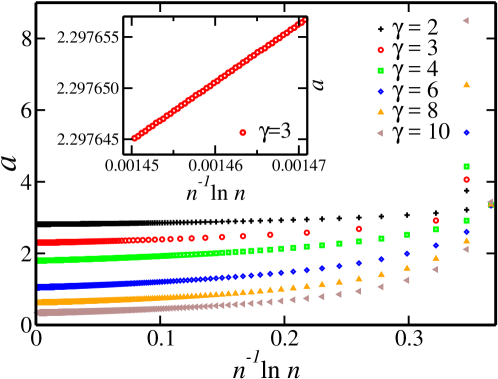
Figure 1: (color online) The variation of $a(n)$, as defined in Eq. (80), with $n^{-1}\ln n$ for stretched exponential noise distribution, as defined in Eq. (77), with $b=3$ and for different values of $\gamma$. The inset shows the same quantity, $a(n)$ in the limit of large $n$ (small values of $n^{-1}\ln n$) for $\gamma=3$ to illustrate the linear dependence for large $n$.

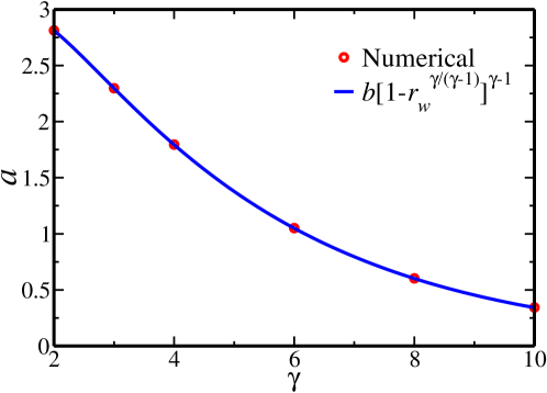
Figure 2: (color online) Comparison of numerical value of the constant $a$, obtained by extrapolating $a(n)$ to $n\to\infty$ [see Fig. 1], with the analytical formula [see Eq. (69)]. The data are for stretched exponential noise distribution, as defined in Eq. (77), with $b=3$ and for different values of $\gamma$.

When $\delta=0$, the moment equation Eq. (3) simplifies to

$$\left[1-\alpha^{2n}-\left(1-\alpha\right)^{2n}+\frac{\lambda_{d}}{2\lambda_{c}}\left(1-r_{w}^{2n}\right)\right]M_{2n}=$$

$$\sum_{k=1}^{n-1}\binom{2n}{2k}\alpha^{2k}(1-\alpha)^{2n-2k}M_{2k}M_{2n-2k}$$

$$+\frac{\lambda_{d}}{2\lambda_{c}}\sum_{k=1}^{n}\binom{2n}{2k}r_{w}^{2n-2k}M_{2n-2k}N_{2k},$$ (75)

where $N_{i}$ is the $i$-th moment of the noise distribution, and

$$M_{2n}\equiv\langle v^{2n}\rangle,\quad n=1,2,\ldots.$$ (76)

This relation expresses a moment in terms of lower order moments. Thus, by knowing $M_{0}=1$, higher order moments may be obtained by iteration.

We will consider normalized stretched exponential distributions for the noise distribution $\Phi(\eta)$:

$$\Phi(\eta)=\frac{b^{\frac{1}{\gamma}}}{2\Gamma\left(1+\frac{1}{\gamma}\right)}\exp(-b|\eta|^{\gamma}),~{}~{}~{}b,\gamma>0.$$ (77)

for which the moments are

$$N_{2n}=b^{-2n/\gamma}\frac{\Gamma(\frac{2n+1}{\gamma})}{\gamma\Gamma(1+\frac{1}{\gamma})}.$$ (78)

Consider now the velocity distribution as derived in this paper [see Eq. (1)] $P(v)\sim\exp(-a|v|^{\gamma}-a^{\prime}(\ln|v|)^{2})$. For this distribution, from Eq. (20) with $\delta=0$, it is straightforward to show that the ratio of consecutive moments has the form

$$\Delta_{n}\equiv\frac{M_{2n+2}}{M_{2n}}=\left(\frac{2n}{a\gamma}\right)^{\frac{2}{\gamma}}\left[1-\frac{2a^{\prime}}{\gamma^{2}}\frac{\ln n}{n}+\mathcal{O}\left(\frac{1}{n}\right)\right].$$ (79)

By measuring $\Delta_{n}$ for large $n$, it was shown in Ref. Prasad:17 that $\beta=\gamma$. Here, we focus on determining $a$ and $a_{1}$ numerically and comparing with Eq. (1). In Fig. 1, we show the variation of the numerically computed

$$a(n)=\frac{2n}{\gamma\Delta_{n}^{\gamma/2}},$$ (80)

with $\ln n/n$. The data for each $\gamma>1$ lie on a straight line which when extrapolated to infinite $n$ gives the numerical estimate for $a$. Figure 2 compares the numerically obtained value with the analytically obtained expression, and we find an excellent agreement.

Now, we determine the constant $a^{\prime}$ by assuming that the expression for $a$ is exact. In that case, we define

$$\frac{2a^{\prime}(n)}{\gamma^{2}}=\frac{n}{\ln n}\left[1-\Delta_{n}\left(\frac{a\gamma}{2n}\right)^{\frac{2}{\gamma}}\right]$$ (81)

such that $a^{\prime}=a^{\prime}(n)+\mathcal{O}(1/\ln n)$. The variation of $a^{\prime}(n)$ with $1/\ln n$ is shown in Fig. 3. For large $n$, the variation is linear. By extrapolating to infinite $n$, we obtain $a^{\prime}$. The extrapolation may be done using a linear or quadratic fit. The results for both extrapolations are shown in Fig. 4 and compared with the analytically obtained result [Eq. (73)] when $\tilde{\xi}=0,~{}\tilde{\delta}=0$]. There is excellent agreement.

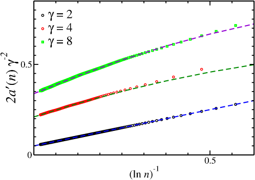
Figure 3: (color online) The variation of numerical value of $2a^{\prime}(n)/\gamma^{2}$, as defined in Eq. (81), with $[\ln n]^{-1}$ for stretched exponential noise distribution, as defined in Eq. (77), with $b=3$ and for different values of $\gamma$. The quadratic fits to the data are shown by dashed lines.

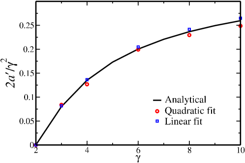
Figure 4: (color online) Comparison of numerical value of the constant $2a^{\prime}/\gamma^{2}$, obtained by extrapolating $2a^{\prime}(n)/\gamma^{2}$ to $n\to\infty$ [see Fig. 3], with the analytical formula [see Eq. (73) with $\tilde{\chi}=0,~{}\tilde{\delta}=0$] for two different extrapolation schemes. The data are for stretched exponential noise distribution, as defined in Eq. (77), with $b=3$ and for different values of $\gamma$.

5 Summary and conclusions

In summary, we derived analytical results for the asymptotic behavior of the velocity distribution for a driven inelastic granular gas with one-dimensional scalar velocity. Each pair of particles undergo inelastic collisions as described in Eq. (8), at a rate that depends on the relative velocity $\Delta v$ as $|\Delta v|^{\delta}$. Each particle is driven at a constant rate by dissipative driving as described in Eq. (10), and is characterized by the dissipation parameter $r_{w}$. To perform our analysis of the moment equation, we assume that the leading asymptotic behaviour of the velocity distribution is a stretched exponential. We then obtain self-consistent solutions that are consistent with this assumption. We obtain analytical results for arbitrary coefficients of restitution, arbitrary $\delta$, as well as generic noise distributions characterized by a stretched exponential exponent $\gamma$ [see Eq. (15)]. The main results obtained in this paper are summarized in Eqs. (1)–(7). For the dissipative case, $r_{w}<1$, the statistics of the velocity distribution are non-universal in that the stretched exponential exponent $\beta$ is determined solely by the noise distribution. For $r_{w}=1$, the distribution is universal, provided $\gamma>\min[\frac{2+\delta}{2},1]$. In addition to the stretched exponential exponent $\beta$, we also determined the different coefficients that describe the asymptotic behavior of the velocity distribution. Surprisingly, we find the presence of logarithmic corrections to the leading stretched exponential behavior. These corrections could be confirmed through a numerical solution of the exact moment equations for the special case $\delta=0$. We note that there are no exact results for models where $\delta\neq 0$.

In the case of $r_{w}=1$ the solution for the stretched exponential exponent $\beta$ is equal to $(2+\delta)/2$, provided $\delta\leq 0$ and is equal to $1$ for $\delta>0$ albeit with additional logarithmic corrections. The results for $r_{w}=1$ depend sensitively on the values of $\gamma$ and $\delta$ and are summarized in Fig. 5. The expression for $\beta=(2+\delta)/2$, when $-2<\delta\leq 0$, is identical to that obtained in kinetic theory. However, while this result continues to also hold for positive $\delta$ in kinetic theory, our calculations show that $\beta=1$ for $\delta>0$ with logarithmic corrections. Thus, the kinetic theory result of $\beta=3/2$ for $\delta=1$ (ballistic motion) cannot be obtained from the solution presented in the current paper. However, if we had incorrectly truncated the expression for moments of noise in Eq. (36) to only the first term, then the kinetic theory result would be recovered. In terms of the master equation for the velocity distribution, the difference between kinetic theory result and our results can be traced to the diffusive driving term in kinetic theory, that is obtained by truncating the Taylor expansion of the last term in Eq. (11), in terms of derivatives of the velocity distribution $P(v)$, up to only the second derivative. However, it may be shown that this truncation is not valid when $\delta>0$, and maximal term in the Taylor expansion is a term corresponding to a higher order derivative [see Appendix B for details of this analysis].

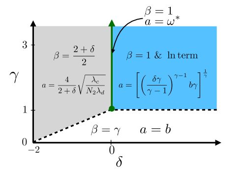
Figure 5: (color online) Summary of results for the stretched exponential exponent $\beta$ and the parameter $a$ as a function of the parameters $\gamma$ and $\delta$, for the case $r_{w}=1$.

There is, however, a special limit in which the kinetic theory results may be recovered. Consider Eqs. (36), (37), and (38) describing the relation between moments of velocity and moments of noise. Suppose in Eq. (38), the limit $N_{2}\to 0$, where $N_{2}$ is the second moment of the noise distribution, is taken before the limit $n\to\infty$ is taken. Then $N_{4}/N_{2}\to 0$, and Eq. (36) may be truncated by keeping only the first term on the right hand side. For a sensible limit we need to take $\lambda_{d}\to\infty$ keeping $\lambda_{d}N_{2}$ fixed. For this special limit, we then obtain, for $r_{w}=1$, the kinetic theory result $\beta=(2+\delta)/2$.

This special limit was also considered in Ref. Prasad:14 , where the driving mechanism (see Eq. (10)), in the limit of diffusive driving, was shown to be an Ornstein-Uhlenbeck when the noise distribution is a gaussian Prasad:14 . In particular, the limit taken was $r_{w}\to\pm 1$ such that $(1\pm r_{w})\lambda_{d}\to\Gamma$, and $N_{2}\to 0$, $\lambda_{d}\to\infty$ keeping $\lambda_{d}N_{2}$ fixed. We note that in Ref. Prasad:14 , only the case $r_{w}\to-1$ was considered, but it is straightforward to see that the derivation goes through for $r_{w}\to 1$ also. For non-gaussian noise, as considered in the current paper, the derivation still goes through because in this limit, central limit theorem ensures that the noise arising from repeated driving ($\lambda_{d}\to\infty$) is a gaussian. On including the dominant term arising from collisions, the resultant master equation for the steady state velocity distribution has the form

$$-c_{1}v^{\delta}P(v)+c_{2}\frac{\partial^{2}}{\partial v^{2}}P(v)+\Gamma\frac{\partial}{\partial v}[vP(v)]=0,$$ (82)

where $c_{1}$ and $c_{2}$ are constants. It is straightforward to see that, by balancing the second and third terms and ignoring inter-particle collisions, one obtains $\beta=2$ Montanero:00 ; Biben02 ; Villani:06 . On the other hand, when $r_{w}=1$, then $\Gamma=0$, and on balancing the first and third terms, one obtains $\beta=(2+\delta)/2$ as in kinetic theory Ernst2003 .

The analysis of the moment equation was performed under the assumption that the leading asymptotic behaviour of the velocity distribution is a stretched exponential. We then obtain self-consistent solutions that are consistent with this assumption. Thus, we are unable to show that the solutions that we obtain are unique, as there may be other self-consistent solutions with a different ansatz for the velocity distribution. However, the results that we obtain are in excellent agreement with the numerical results for the case $\delta=0$. Thus, we believe that the results obtained in the paper may well be exact.

The results for the one dimensional driven granular gas obtained in this paper suggest that the velocity distribution is determined mostly by the noise distribution and hence the hope for a universal distribution is misplaced. However, the one-dimensional gas is different from a granular gas in higher dimensions as now the possibility of collisions which are not just head on are allowed. In a recent paper, we have shown that, by extending the above analysis to a two-dimensional system, the velocity distribution becomes universal with $\beta=2$ albeit with logarithmic corrections Prasad:19 .

Appendix A Large moments of the velocity distribution

We determine the behavior of large moments when the velocity distribution has the asymptotic form:

$$P(v)\sim e^{-a|v|^{\beta}+\Psi(v)},~{}~{}|v|\to\infty,~{}a>0.$$ (83)

where $v^{-\beta}\Psi(|v|)\to 0$ for $|v|\to\infty$. The aim is to determine the moment $\langle|v_{1}-v_{2}|^{\delta}v_{1}^{2n-k}v_{2}^{k}\rangle$ for large $n$ and $k$. In the limit $k\propto n$, we change variables to $k=xn$ with $0\leq x\leq 1$, to obtain

$$\langle|v_{1}-v_{2}|^{\delta}v_{1}^{2n-k}v_{2}^{k}\rangle\sim\int dv_{1}dv_{2}|v_{1}-v_{2}|^{\delta}v_{1}^{(2-x)n}v_{2}^{xn}$$

$$\times e^{-a|v_{1}|^{\beta}-a|v_{2}|^{\beta}+\Psi(v_{1})+\Psi(v_{2})}\hskip 22.76228pt$$ (84)

Rescaling the integration variables $v_{1}$, and $v_{2}$ as $v_{1}=n^{1/\beta}t_{1}$ and $v_{2}=n^{1/\beta}t_{2}$, Eq. (84) simplifies to

$$\langle|v_{1}-v_{2}|^{\delta}v_{1}^{2n-k}v_{2}^{k}\rangle \sim n^{\frac{2+\delta+2n}{\beta}}\int dt_{1}dt_{2}e^{n[f(t_{1})+g(t_{2})]}\times$$

$$|t_{1}-t_{2}|^{\delta}e^{\Psi(n^{1/\beta}t_{1})+\Psi(n^{1/\beta}t_{2})}$$ (85)

where,

$$\begin{split}f(t_{1})&=-at_{1}^{\beta}+(2-x)\ln t_{1},\\ g(t_{2})&=-at_{2}^{\beta}+x\ln t_{2}.\end{split}$$ (86)

The integral in Eq. (85) may be evaluated using the saddle point approximation by maximizing $f(t_{1})$ and $g(t_{2})$ with respect to $t_{1}$ and $t_{2}$. Setting $df(t_{1})/dt_{1}=0$ and $dg(t_{2})/dt_{2}=0$, we obtain the solution $t_{1}^{*}$ and $t_{2}^{*}$ to be

$$t_{1}^{*} =\left(\frac{2-x}{a\beta}\right)^{\frac{1}{\beta}},$$ (87)

$$t_{2}^{*} =\left(\frac{x}{a\beta}\right)^{\frac{1}{\beta}},$$ (88)

and

$$\begin{split}f(t_{1}^{*})&=\frac{2-x}{\beta}\ln\left(\frac{2-x}{ae\beta}\right),\\ g(t_{2}^{*})&=\frac{x}{\beta}\ln\left(\frac{x}{ae\beta}\right).\end{split}$$ (89)

Doing the saddle point integration in Eq. (85), we obtain

$$\langle|v_{1}-v_{2}|^{\delta}v_{1}^{2n-k}v_{2}^{k}\rangle\sim\frac{n^{\frac{2+\delta}{\beta}}}{n}\left(\frac{n}{2ae\beta}\right)^{\frac{2n}{\beta}}\times\hskip 28.45274pt$$

$$e^{n\left[\frac{2-x}{\beta}\ln(2-x)+\frac{x}{\beta}\ln x\right]}e^{\Psi(n^{1/\beta}t_{1}^{*})+\Psi(n^{1/\beta}t_{2}^{*})},$$ (90)

where the extra factor of $n$ appears in the denominator of the left hand side of Eq. (90) because of the two-dimensional saddle point integration.

In a similar way one can find the asymptotic form for $\langle|v_{1}-v_{2}|^{\delta}v_{1}^{2n}\rangle$ for large $n$. Consider the equality,

$$\langle|v-v_{1}|^{\delta}v^{2n}\rangle=\int dvdv_{1}P(v)P(v_{1})|v-v_{1}|^{\delta}v^{2n}.$$ (91)

As we are interested in the large $n$, the moments are dominated by values of $|v|$. In this limit it is possible to approximate, $|v-v_{1}|\approx|v|$, and Eq. (91) reduces to

$$\langle|v-v_{1}|^{\delta}v^{2n}\rangle\sim\int dvP(v)|v|^{2n+\delta}.$$ (92)

Doing a transformation, $v=n^{1/\beta}t$ as before, we obtain

$$\langle|v-v_{1}|^{\delta}v^{2n}\rangle\sim n^{\frac{1+\delta}{\beta}}\int dte^{nf(t)+\Psi(n^{1/\beta}t)}n^{2n/\beta}$$ (93)

where,

$$f(t)=-at^{\beta}+2\ln t$$ (94)

Doing a saddle point integration with respect to $t$, by maximizing $f(t)$, one obtains,

$$\langle|v-v_{1}|^{\delta}v^{2n}\rangle\approx n^{\frac{1+\delta}{\beta}}\sqrt{\frac{2\pi}{f^{\prime\prime}(t^{*})n}}{t^{*}}^{\delta}\left(\frac{2n}{ae\beta}\right)^{\frac{2n}{\beta}}e^{\Psi(n^{\frac{1}{\beta}}t^{*})}~{}~{}$$ (95)

where we have substituted, the maximal value of $f(t)$,

$$f(t^{*})=\frac{2}{\beta}\ln\left(\frac{2}{ae\beta}\right),$$ (96)

and

$$t^{*}=\left(\frac{2}{a\beta}\right)^{\frac{1}{\beta}}.$$ (97)

The same calculation may be used to determine the asymptotic behavior of the noise distribution. Considering the noise distribution with the form as in Eq. (15),

$$\Phi(\eta)\sim|\eta|^{\tilde{\chi}}e^{-b|\eta|^{\gamma}}\text{for}|\eta|^{2}\gg\langle\eta^{2}\rangle_{\Phi},$$ (98)

then

$$N_{2n}=\langle\eta^{2n}\rangle\approx n^{\frac{1+\tilde{\chi}}{\gamma}}\sqrt{\frac{2\pi}{g^{\prime\prime}(y^{*})n}}{y^{*}}^{\tilde{\chi}}\left[\frac{2n}{be\gamma}\right]^{\frac{2n}{\gamma}}.$$ (99)

where,

$$g(y)=-by^{\gamma}+2\ln y$$ (100)

and

$$y^{*}=\left(\frac{2}{b\gamma}\right)^{\frac{1}{\gamma}}.$$ (101)

Appendix B Taylor expansion of the terms in Eq. (11) arising from driving

In this appendix, we analyse the terms [the last two terms] of Eq. (11) arising from driving – which we denote by $I$ – for $r_{w}=1$:

$$I=-\lambda_{d}P(v)+\lambda_{d}\int\int d\eta dv_{1}\Phi(\eta)P(v_{1})\delta\left[-v_{1}+\eta-v\right],$$ (102)

by Taylor expanding the term in the integrand, and using the solution for the velocity distribution that we have obtained in the paper to identify the most dominant term in the expansion. Integrating over $v_{1}$, we obtain

$$I=-\lambda_{d}P(v)+\lambda_{d}\int d\eta\Phi(\eta)P(v-\eta).$$ (103)

Taylor expanding $P(v-\eta)$ about $\eta=0$ and integrating over $\eta$, Eq. (103) reduces to

$$I=\lambda_{d}\sum_{k=1}^{\infty}\frac{\langle\eta^{2k}\rangle}{(2k)!}\frac{d^{2k}}{dv^{2k}}P(v)\equiv\sum_{k=1}^{\infty}t_{k}.$$ (104)

We now determine the dominant term in this expansion, given that $P(v)$ has the asymptotic behaviour as given in Eqs. (3)-(7).

From Eqs. (3)-(7), the velocity distribution has the asymptotic form

$$\ln P(v)\sim-a|v|^{\beta}(\ln|v|)^{\theta},\quad|v|\to\infty,$$ (105)

where $\theta>0$ for $\gamma>1$, $\delta>0$, and $\theta=0$ otherwise. Thus,

$$\frac{d^{2k}}{dv^{2k}}P(v)\approx\left[a\beta v^{\beta-1}(\ln|v|)^{\theta}\right]^{2k}P(v),\quad|v|\to\infty.$$ (106)

The asymptotic form for the moments of $\eta$ is given in Eq. (22). Using these asymptotic forms, we obtain the ratio of successive terms in Eq. (104) to be

$$\frac{t_{k+1}}{t_{k}}\approx\left(\frac{2}{b\gamma}\right)^{\frac{2}{\gamma}}\frac{\left[a\beta v^{\beta-1}(\ln|v|)^{\theta}\right]^{2}}{4}k^{\frac{2(1-\gamma)}{\gamma}}.$$ (107)

We now analyse Eq. (107) for different cases.

Case I – $\delta\leq 0$: From Eq. (3), we know that $\theta=0$ and $\beta=\min\left[\frac{2+\delta}{2},\gamma\right]$. When $\delta<0$, then $\beta<1$. Thus, for large $v$, the ratio in Eq. (107) is much smaller than $1$ for small $k$. Also, for $\gamma>1$, the ratio decreases with $k$. Thus, the truncation at the first term is valid, and the expression for $\beta$ may be obtained from the continuum equations. However, when $\gamma<1$, it is possible that the expansion may break down as there could be contribution from large derivatives. Indeed, from comparing with our analytic solution, for $\gamma<1+\delta/2$, the Taylor expansion about small $\eta$ breaks down. When $\delta=0$, then $\beta=1$. For $\gamma>1$, the most dominant term in the expansion, determined by $t_{k+1}/t_{k}=1$, is a $k^{*}$ that is independent of $v$. Then, it is straightforward to show that $\beta=1$ is a consistent solution. Thus, while the dominant term in the expansion is not the first term, the result obtained from the continuum equations do not change.

Case II – $\delta>0$: Now, for $\gamma>1$, the solution of $t_{k^{*}+1}/t_{k^{*}}=1$ is given by $k^{*}\propto(\ln|v|)^{\frac{\theta\gamma}{\gamma-1}}$. Now, $k^{*}$ depends on $v$, and it is clear that truncating the Taylor expansion at the first term will lead to wrong results. In fact, truncating at the first term gives $\beta=(2+\delta)/2$, while we have derived, without making any approximations, $\beta=1$.

References

- [1] Heinrich M. Jaeger, Sidney R. Nagel, and Robert P. Behringer. Granular solids, liquids, and gases. Rev. Mod. Phys., 68:1259–1273, Oct 1996.
- [2] Igor S. Aranson and Lev S. Tsimring. Patterns and collective behavior in granular media: Theoretical concepts. Rev. Mod. Phys., 78:641–692, Jun 2006.
- [3] I. Goldhirsch and G. Zanetti. Clustering instability in dissipative gases. Phys. Rev. Lett., 70:1619–1622, Mar 1993.
- [4] J. Li, I. S. Aranson, W.-K. Kwok, and L. S. Tsimring. Periodic and disordered structures in a modulated gas-driven granular layer. Phys. Rev. Lett., 90:134301, Apr 2003.
- [5] Eric I Corwin, Heinrich M Jaeger, and Sidney R Nagel. Structural signature of jamming in granular media. Nature, 435(7045):1075–1078, 2005.
- [6] A. Prados and E. Trizac. Kovacs-like memory effect in driven granular gases. Phys. Rev. Lett., 112:198001, May 2014.
- [7] Antonio Lasanta, Francisco Vega Reyes, Antonio Prados, and Andrés Santos. When the hotter cools more quickly: Mpemba effect in granular fluids. Phys. Rev. Lett., 119:148001, Oct 2017.
- [8] Jilmy P Joy, Sudhir N Pathak, Dibyendu Das, and R Rajesh. Shock propagation in locally driven granular systems. Physical Review E, 96(3):032908, 2017.
- [9] J. Javier Brey, M. J. Ruiz-Montero, and D. Cubero. Homogeneous cooling state of a low-density granular flow. Phys. Rev. E, 54:3664–3671, Oct 1996.
- [10] Sergei E. Esipov and Thorsten Pöschel. The granular phase diagram. J. Stat. Phys., 86(5):1385–1395, 1997.
- [11] E. Ben-Naim, S. Y. Chen, G. D. Doolen, and S. Redner. Shocklike dynamics of inelastic gases. Phys. Rev. Lett., 83:4069–4072, Nov 1999.
- [12] E. Ben-Naim and P. L. Krapivsky. Multiscaling in inelastic collisions. Phys. Rev. E, 61:R5–R8, Jan 2000.
- [13] Xiaobo Nie, Eli Ben-Naim, and Shiyi Chen. Dynamics of freely cooling granular gases. Phys. Rev. Lett., 89:204301, Oct 2002.
- [14] Supravat Dey, Dibyendu Das, and R Rajesh. Lattice models for ballistic aggregation in one dimension. Europhys. Lett., 93(4):44001, 2011.
- [15] Sudhir N. Pathak, Dibyendu Das, and R. Rajesh. Inhomogeneous cooling of the rough granular gas in two dimensions. Europhys. Lett., 107(4):44001, 2014.
- [16] Sudhir N. Pathak, Zahera Jabeen, Dibyendu Das, and R. Rajesh. Energy decay in three-dimensional freely cooling granular gas. Phys. Rev. Lett., 112:038001, Jan 2014.
- [17] Mahendra Shinde, Dibyendu Das, and R Rajesh. Violation of the porod law in a freely cooling granular gas in one dimension. Phys. Rev. Lett., 99(23):234505, 2007.
- [18] Subhajit Paul and Subir K. Das. Dynamics of clustering in freely cooling granular fluid. Europhys. Lett., 108(6):66001, 2014.
- [19] Subhajit Paul and Subir K. Das. Ballistic aggregation in systems of inelastic particles: Cluster growth, structure, and aging. Phys. Rev. E, 96:012105, Jul 2017.
- [20] Nikolai V Brilliantov, Arno Formella, and Thorsten Pöschel. Increasing temperature of cooling granular gases. Nat. Comm., 9(1):797, 2018.
- [21] J. S. van Zon and F. C. MacKintosh. Velocity distributions in dissipative granular gases. Phys. Rev. Lett., 93:038001, Jul 2004.
- [22] Christian Scholz and Thorsten Pöschel. Velocity distribution of a homogeneously driven two-dimensional granular gas. Phys. Rev. Lett., 118(19):198003, 2017.
- [23] CRK Windows-Yule. Do granular systems obey statistical mechanics? a review of recent work assessing the applicability of equilibrium theory to vibrationally excited granular media. Int. J. Mod. Phys. B, 31(10):1742010, 2017.
- [24] E. Clement and J. Rajchenbach. Fluidization of a bidimensional powder. Europhys. Lett., 16(2):133, 1991.
- [25] Stephen Warr, Jonathan M. Huntley, and George T. H. Jacques. Fluidization of a two-dimensional granular system: Experimental study and scaling behavior. Phys. Rev. E, 52:5583–5595, Nov 1995.
- [26] A. Kudrolli, M. Wolpert, and J. P. Gollub. Cluster formation due to collisions in granular material. Phys. Rev. Lett., 78:1383–1386, Feb 1997.
- [27] J. S. Olafsen and J. S. Urbach. Clustering, order, and collapse in a driven granular monolayer. Phys. Rev. Lett., 81:4369–4372, Nov 1998.
- [28] J. S. Olafsen and J. S. Urbach. Velocity distributions and density fluctuations in a granular gas. Phys. Rev. E, 60:R2468–R2471, Sep 1999.
- [29] W. Losert, D. G. W. Cooper, J. Delour, A. Kudrolli, and J. P. Gollub. Velocity statistics in excited granular media. Chaos, 9(3):682–690, 1999.
- [30] A. Kudrolli and J. Henry. Non-gaussian velocity distributions in excited granular matter in the absence of clustering. Phys. Rev. E, 62:R1489–R1492, Aug 2000.
- [31] Florence Rouyer and Narayanan Menon. Velocity fluctuations in a homogeneous 2d granular gas in steady state. Phys. Rev. Lett., 85:3676–3679, Oct 2000.
- [32] Daniel L. Blair and A. Kudrolli. Velocity correlations in dense granular gases. Phys. Rev. E, 64:050301, Oct 2001.
- [33] J. S. van Zon, J. Kreft, Daniel I. Goldman, D. Miracle, J. B. Swift, and Harry L. Swinney. Crucial role of sidewalls in velocity distributions in quasi-two-dimensional granular gases. Phys. Rev. E, 70:040301, Oct 2004.
- [34] Pedro M Reis, Rohit A Ingale, and Mark D Shattuck. Forcing independent velocity distributions in an experimental granular fluid. Phys. Rev. E, 75(5):051311, 2007.
- [35] Hong-Qiang Wang, Klebert Feitosa, and Narayanan Menon. Particle kinematics in a dilute, three-dimensional, vibration-fluidized granular medium. Phys. Rev. E, 80(6):060304, 2009.
- [36] Alexandre Vilquin, Hamid Kellay, and Jean-François Boudet. Shock waves induced by a planar obstacle in a vibrated granular gas. J. Fluid Mech., 842:163–187, 2018.
- [37] Ricky D Wildman, J Beecham, and TL Freeman. Granular dynamics of a vibrated bed of dumbbells. Eur. Phys. J. Special Topics, 179(1):5–17, 2009.
- [38] GW Baxter and JS Olafsen. Kinetics: Gaussian statistics in granular gases. Nature, 425(6959):680–680, 2003.
- [39] GW Baxter and JS Olafsen. The temperature of a vibrated granular gas. Granular Matter, 9(1-2):135–139, 2007.
- [40] CRK Windows-Yule and DJ Parker. Boltzmann statistics in a three-dimensional vibrofluidized granular bed: Idealizing the experimental system. Phys. Rev. E, 87(2):022211, 2013.
- [41] I. S. Aranson and J. S. Olafsen. Velocity fluctuations in electrostatically driven granular media. Phys. Rev. E, 66:061302, Dec 2002.
- [42] K. Kohlstedt, A. Snezhko, M. V. Sapozhnikov, I. S. Aranson, J. S. Olafsen, and E. Ben-Naim. Velocity distributions of granular gases with drag and with long-range interactions. Phys. Rev. Lett., 95:068001, Aug 2005.
- [43] Malte Schmick and Mario Markus. Gaussian distributions of rotational velocities in a granular medium. Phys. Rev. E, 78(1):010302, 2008.
- [44] E. Falcon, J.-C. Bacri, and C. Laroche. Equation of state of a granular gas homogeneously driven by particle rotations. Europhys. Lett., 103(6):64004, 2013.
- [45] Soichi Tatsumi, Yoshihiro Murayama, Hisao Hayakawa, and Masaki Sano. Experimental study on the kinetics of granular gases under microgravity. J. Fluid Mech., 641:521–539, 2009.
- [46] M Hou, R Liu, G Zhai, Z Sun, K Lu, Yves Garrabos, and Pierre Evesque. Velocity distribution of vibration-driven granular gas in knudsen regime in microgravity. Microgravity Sci. Technol., 20(2):73, 2008.
- [47] Yan Grasselli, Georges Bossis, and Romain Morini. Translational and rotational temperatures of a 2d vibrated granular gas in microgravity. Eur. Phys. J. E, 38(2):8, 2015.
- [48] A Puglisi, V Loreto, U Marini Bettolo Marconi, A Petri, and A Vulpiani. Clustering and non-gaussian behavior in granular matter. Phys. Rev. Lett., 81(18):3848, 1998.
- [49] A Puglisi, V Loreto, U Marini Bettolo Marconi, and A Vulpiani. Kinetic approach to granular gases. Phys. Rev. E, 59(5):5582, 1999.
- [50] Sung Joon Moon, M. D. Shattuck, and J. B. Swift. Velocity distributions and correlations in homogeneously heated granular media. Phys. Rev. E, 64:031303, Aug 2001.
- [51] J. S. van Zon and F. C. MacKintosh. Velocity distributions in dilute granular systems. Phys. Rev. E, 72:051301, Nov 2005.
- [52] R. Cafiero, S. Luding, and H. J. Herrmann. Rotationally driven gas of inelastic rough spheres. Europhys. Lett., 60(6):854, 2002.
- [53] Alexis Burdeau and Pascal Viot. Quasi-gaussian velocity distribution of a vibrated granular bilayer system. Phys. Rev. E, 79(6):061306, 2009.
- [54] Bishakdatta Gayen and Meheboob Alam. Orientational correlation and velocity distributions in uniform shear flow of a dilute granular gas. Phys. Rev. Lett., 100(6):068002, 2008.
- [55] Bishakhdatta Gayen and Meheboob Alam. Effect of coulomb friction on orientational correlation and velocity distribution functions in a sheared dilute granular gas. Phys. Rev. E, 84(2):021304, 2011.
- [56] Li Rui, Zhang Duan-Ming, and Li Zhi-Hao. Velocity distributions in inelastic granular gases with continuous size distributions. Chin. Phys. Lett., 28(9):090506, 2011.
- [57] Prasenjit Das, Sanjay Puri, and Moshe Schwartz. Granular fluids with solid friction and heating. Granular Matter, 20(1):15, Jan 2018.
- [58] W Kang, Jonathan Machta, and E Ben-Naim. Granular gases under extreme driving. Europhys. Lett., 91(3):34002, 2010.
- [59] Nikolai Brilliantov and Thorsten Pöschel. Kinetic theory of granular gases. Oxford University Press, USA, 2004.
- [60] A. V. Bobylev, J. A. Carrillo, and I. M. Gamba. On some properties of kinetic and hydrodynamic equations for inelastic interactions. J. Stat. Phys., 98(3):743–773, Feb 2000.
- [61] T.P.C. van Noije and M.H. Ernst. Velocity distributions in homogeneous granular fluids: the free and the heated case. Granular Matter, 1(2):57–64, 1998.
- [62] M. H. Ernst and R. Brito. Driven inelastic maxwell models with high energy tails. Phys. Rev. E, 65:040301, Mar 2002.
- [63] T. Antal, Michel Droz, and Adam Lipowski. Exponential velocity tails in a driven inelastic maxwell model. Phys. Rev. E, 66:062301, Dec 2002.
- [64] A. Santos and M. H. Ernst. Exact steady-state solution of the boltzmann equation: A driven one-dimensional inelastic maxwell gas. Phys. Rev. E, 68:011305, Jul 2003.
- [65] Matthieu H. Ernst and Ricardo Brito. Asymptotic Solutions of the Nonlinear Boltzmann Equation for Dissipative Systems. Springer Berlin Heidelberg, Berlin, Heidelberg, 2003.
- [66] MH Ernst, E Trizac, and A Barrat. The rich behavior of the boltzmann equation for dissipative gases. Europhys. Lett., 76(1):56, 2006.
- [67] M. H. Ernst, E. Trizac, and A. Barrat. The boltzmann equation for driven systems of inelastic soft spheres. Journal of Statistical Physics, 124(2):549–586, Aug 2006.
- [68] Alain Barrat, E Trizac, and MH Ernst. Quasi-elastic solutions to the nonlinear boltzmann equation for dissipative gases. J. Phys. A, 40(15):4057, 2007.
- [69] Cédric Villani. Mathematics of granular materials. Journal of statistical physics, 124(2):781–822, 2006.
- [70] V. V. Prasad, Sanjib Sabhapandit, and Abhishek Dhar. High-energy tail of the velocity distribution of driven inelastic maxwell gases. Europhys. Lett., 104(5):54003, 2013.
- [71] V. V. Prasad, Dibyendu Das, Sanjib Sabhapandit, and R. Rajesh. Velocity distribution of a driven inelastic one-component maxwell gas. Phys. Rev. E, 95:032909, Mar 2017.
- [72] V V Prasad, Dibyendu Das, Sanjib Sabhapandit, and R Rajesh. Velocity distribution of driven granular gases. Journal of Statistical Mechanics: Theory and Experiment, 2019(6):063201, jun 2019.
- [73] V. V. Prasad, Sanjib Sabhapandit, and Abhishek Dhar. Driven inelastic maxwell gases. Phys. Rev. E, 90:062130, Dec 2014.
- [74] María José Montanero and Andrés Santos. Computer simulation of uniformly heated granular fluids. Granular Matter, 2(2):53–64, 2000.
- [75] Thierry Biben, Ph.A. Martin, and J. Piasecki. Stationary state of thermostated inelastic hard spheres. Physica A, 310(3):308 – 324, 2002.