Lévy area of fractional Ornstein-Uhlenbeck process and parameter estimation

Abstract

In this paper, we study the estimation problem of an unknown drift parameter matrix for fractional Ornstein-Uhlenbeck process in multi-dimensional setting. By using rough path theory, we propose pathwise rough path estimators based on both continuous and discrete observations of a single path. The approach is applicable to the high-frequency data. To formulate the parameter estimators, we define a theory of pathwise Itô integrals with respect to fractional Brownian motion. By showing the regularity of fractional Ornstein-Uhlenbeck processes and the long time asymptotic behaviour of the associated Lévy area processes, we prove that the estimators are strong consistent and pathwise stable. Numerical studies and simulations are also given in this paper.

Keywords. Rough path estimator, Pathwise stability, Fractional Brownian motions,

FOU processes, Itô integration, Lévy area, Long time asymptotic, High-frequency data.

MSC[2010]. 60H05, 62F12, 62M09, 91G30.

1 Introduction

The statistical analysis of time series and random processes, parameter estimations, non-parameter estimations and statistical inferences, has been mainly concentrated on models described in terms of diffusion processes and semi-martingales, see e.g. some standard references such as [23, 21, 35, 36] and etc. Models which are not semi-martingales have received some attention in applications where long-time memory effects have to be taken into consideration, see e.g. [22, 38, 19] for example. In this article, we study multi-dimensional Ornstein-Uhlenbeck processes (OU processes for short) driven by fractional Brownian motions (fBM), known in recent literature as fractional Ornstein-Uhlenbeck processes (fOU processes for simplicity), defined to be the solution of the stochastic differential equation (SDE)

$$dX_{t}=-\Gamma X_{t}dt+\Sigma dB_{t}^{H},\ X_{0}=x_{0},$$ (1.1)

where $B^{H}$ is a $d$-dimensional fBM with Hurst parameter $H\in(0,1)$, $\Gamma\in\mathbb{R}^{d\times d}$ is the drift matrix and $\Sigma\in\mathbb{R}^{d\times d}$ is the volatility matrix which is non-degenerate. The previous SDE has to be interpreted as the stochastic integral equation

$$X_{t}=x_{0}-\int_{0}^{t}\Gamma X_{s}ds+\Sigma B_{t}^{H},$$

which has an unique solution given by

$$X_{t}=e^{-\Gamma t}x_{0}+\int_{0}^{t}e^{-\Gamma(t-s)}\Sigma dB_{s}^{H}.$$ (1.2)

The integral on the right hand side is understood as an Young’s integral. Therefore, like ordinary OU processes, $(X_{t})$ is a Gaussian process.

Equation (1.1) can be used to describe systems with linear interactions perturbed by Gaussian noise. An example of applications is inter-banking lending, see e.g. [8, 14]. In applications, an important question is to estimate the interaction structure $\Gamma$ from an observation of a single path of the process, assuming that $\Sigma$ is known and a single path $X(\omega)$ can be observed continuously or at discrete time.

For one dimensional case, the maximum likelihood estimator (MLE) and the least square estimator (LSE) and their properties have been studied in literature, see e.g. [22, 38, 19, 20]. Kleptsyna and Le Breton [22] and Tudor and Viens [38] have studied the maximum likelihood estimator based on continuous observation and obtained the strong consistency of the MLE as $T$ goes to infinity. Hu and Nualart [19] studied the least square estimator for the case where the Hurst parameter $H>\frac{1}{2}$. The strong consistency as $T\to\infty$ was proved for $H>\frac{1}{2}$ and a central limit theorem was also established if $\frac{1}{2}<H<\frac{3}{4}$. Hu, Nualart and Zhou [20] extended their results for all $H\in(0,1)$.

There are however few works on parameter estimation for multi-dimensional fOU processes. The aim of this paper is therefore to fill this gap. First, for continuous observation of a single path, we give an estimator based on the rough path theory (see e.g. Lyons and Qian [27]). In order to formulate the parameter estimator, we should define an Itô type integration theory for multi-dimensional fBM.

Coutin and Qian [11] proposed a theory of Stratonovich integration for multi-dimensional fBM with $H>\frac{1}{4}$ by using the rough path analysis. It remains an open question to build a rough path theory for fBM with Hurst parameter $H\leq\frac{1}{4}$. Therefore, we consider fBM with Hurst parameter $H$ where $\frac{1}{3}<H\leq\frac{1}{2}$. For this case, both fBM and fOU processes are of finite $p$-variation with $2\leq p<3$, and can be enhanced canonically to be geometric rough paths. We may define Itô type integrals with respect to fBM and fOU processes by correcting their enhanced Lévy area processes, and apply it to the study of the parameter estimation problem for fOU processes based on continuous observation. In order to show that the parameter estimator is strongly consistent, we study the regularity of fOU processes and long time asymptotic behaviours of their Lévy area processes, which we believe are of interests by their own.

We also study the estimation problem based on discrete observation. In applications, observation times are discrete rather than continuous, though the sampling frequency can be made to tend to infinity, which is the case for high-frequency financial data. For the statistical inference in this direction, we recommend [1, 2, 28, 3, 5, 10, 4] and references therein. In this paper, we construct a parameter estimator based on high-frequency discrete observation by using rough path theory, and establish the strong consistence of this estimator. We would like mention that Diehl, Friz and Mai [12] studied the maximum likelihood estimators for diffusion processes via the rough path analysis, and initiated a study of estimators for the fractional case, but only for the case that $H=\frac{1}{2}-\varepsilon$, for small $\varepsilon$.

The approach we present in this paper has several advantages over other methods in the existing literature. First, our estimators are for multi-dimensional fOU processes where the no trivial role played by Lévy area processes may be revealed, which differs fundamentally from the one dimensional case. Second, the parameter estimators are pathwise defined, and can be calculated based on observation of a single path. Third, the parameter estimators are pathwise stable and robust, in the sense that, if two observations are very close according to the so called $p$-variation distance (see the main text below), then their corresponding estimators are close too. Fourth, our estimators can be constructed by both continuous observation and discrete observation, in particular for high-frequency financial data.

Numerical studies and simulations are given in this paper, to demonstrate that the parameter estimators we propose are very good. Let us mention that the approach in this paper can be extended to Ornstein-Uhlenbeck process $X_{t}$ driven by a general Gaussian noise $G_{t}$, so that

$$X_{t}=e^{-\Gamma t}x_{0}+\int_{0}^{t}e^{-\Gamma(t-s)}\Sigma dG_{s}$$ (1.3)

where the integral on the right-hand side is well defined as long as $t\rightarrow G_{t}$ is $\alpha$-Hölder continuous for some $\alpha>0$. Such singular OU processes may be useful in applications.

The paper is organized as follows. In section 2, we recall some preliminaries of the rough path theory and outline a theory of pathwise Itô integrals for both fBM and fOU processes. In section 3, we prove the regularity of fOU process and study long time asymptotics of the associated Lévy area processes. Then we construct a continuous rough path estimator in Section 4. We give a complete proof for almost sure convergence and pathwise stability of this estimator. Then in section 5, the discrete rough path estimator based on high-frequency data is presented. In section 6, we give two concrete experimental examples based on simulated sample paths, and the numerical results are shown there.

2 Rough paths and Itô integration

In this section, we introduce several notations from the rough paths theory, following the standard references [15, 16, 17, 26, 27]. We give a definition of Itô integrales for fBM and fOU processes.

2.1 Preliminary of rough paths

Define the truncated tensor algebra $T^{(2)}(\mathbb{R}^{d})$ by $T^{(2)}(\mathbb{R}^{d}):=\oplus_{n=0}^{2}(\mathbb{R}^{d})^{\otimes n},$ with the convention that $(\mathbb{R}^{d})^{\otimes 0}=\mathbb{R}$, and use $\Delta$ to denote the simplex $\{(s,t):0\leq s<t\leq T\}$. Let $X_{t}$ be a continuous path on interval $[0,T]$ and $\mathbf{X}_{s,t}=(1,X_{s,t},\mathbb{X}_{s,t})$ be an element of space $T^{(2)}(\mathbb{R}^{d})$. Actually, when $X_{t}$ is of finite $p$-variation with $2<p<3$, we may lift it to the space $T^{(2)}(\mathbb{R}^{d})$ as a multiple function. The initial motivation is to define integrals with respect to $X$ by increasing information to $X$. We recall Chen’s identity (algebraic information) and the definition of finite $p$-variation (analysis information).

We call that $\mathbf{X}_{s,t}=(1,X_{s,t},\mathbb{X}_{s,t})$ satisfies Chen’s identity if

$$X_{s,t}=X_{t}-X_{s},$$ (2.1)

$$\mathbb{X}_{s,t}-\mathbb{X}_{s,u}-\mathbb{X}_{u,t}=X_{s,u}\otimes X_{u,t},$$ (2.2)

for all $(s,u),\ (u,t)\in\Delta$.

$\mathbf{X}=(1,X_{s,t},\mathbb{X}_{s,t})$ has finite $p$-variations if

$$\sup_{\mathcal{P}}\sum_{[s,t]\in\mathcal{P}}|X_{s,t}|^{p}<\infty,\ \sup_{\mathcal{P}}\sum_{[s,t]\in\mathcal{P}}|\mathbb{X}_{s,t}|^{p/2}<\infty,$$

where $\mathcal{P}$ is a partition of $[0,T]$. It is equivalent to that there exists a control $\omega(s,t)$ such that

$$|X_{s,t}|\leq\omega(s,t)^{1/p},\ |\mathbb{X}_{s,t}|\leq\omega(s,t)^{2/p},\ \forall(s,t)\in\Delta.$$

A control $\omega$ is a non-negative, continuous, super-additive function on $\Delta$ and satisfies that $\omega(t,t)=0$.

Let $2<p<3$ be a constant. A function $\mathbf{X}=(1,X,\mathbb{X})$ from $\Delta$ to $T^{(2)}(\mathbb{R}^{d})$ is called a $p$-rough path if it has finite $p$-variation, and satisfies Chen’s identity. Denote the space of $p$-rough paths as $\Omega_{p}(\mathbb{R}^{d})$.

According to Lyons and Qian [27], the integration operator is defined as a linear map from $\Omega_{p}(\mathbb{R}^{d})$ to $\Omega_{p}(\mathbb{R}^{e})$, i.e. $\int F:\Omega_{p}(\mathbb{R}^{d})\to\Omega_{p}(\mathbb{R}^{e})$, and denote the integral by $Y=\int F(X)d_{\mathfrak{R}}\mathbf{X}$, where

$$Y_{u,v}^{1}\equiv\int_{u}^{v}F(X)d_{\mathfrak{R}_{1}}\mathbf{X}:=\lim_{|\mathcal{P}|\to 0}\sum_{[s,t]\in\mathcal{P}}F(X_{s})X_{s,t}+DF(X_{s})\mathbb{X}_{s,t},$$ (2.3)

and the second level $Y^{2}$ by

$$Y_{u,v}^{2}\equiv\int_{u}^{v}F(X)d_{\mathfrak{R}_{2}}\mathbf{X}:=\lim_{|\mathcal{P}|\to 0}\sum_{[s,t]\in\mathcal{P}}Y_{u,s}^{1}\otimes Y_{s,t}^{1}+F(X_{s})\otimes F(X_{s})\mathbb{X}_{s,t},$$ (2.4)

where the limit takes over all finite partitions $\mathcal{P}$ of interval $[u,v]$.

2.2 FBM as rough paths

Almost all sample paths of a $d$-dimensional fBM with Hurst parameter $H\in(\frac{1}{3},\frac{1}{2}]$ have finite $p$-variation with $2<\frac{1}{H}<p<3$, which can be enhanced canonically to be geometric rough paths. In fact Coutin and Qian [11] constructed the canonical rough path enhancement $\mathbf{B}^{H,\text{Str}}=(1,B^{H},\mathbb{B}^{H,\text{Str}})$ in the Stratonovich sense by using dyadic approximations of fBM and their iterated integrals. But for the parameter estimation problem discussed in this paper, if the stochastic integral in the estimator (see section 4) is understood in the Stratonovich sense, it will almost surely converge to 0. Such estimator is not reasonable and therefore it has no use. So we need a theory of Itô type integration for fBM and fOU process. In [34], the present authors have constructed an Itô type rough path enhancement $\mathbf{B}^{H,\text{It\^{o}}}=(1,B^{H},\mathbb{B}^{H,\text{It\^{o}}})$ associated with an fBM by setting

$$\mathbb{B}_{s,t}^{H,\text{It\^{o}}}=\mathbb{B}_{s,t}^{H,\text{Str}}-\frac{1}{2}I(t^{2H}-s^{2H}),$$

which can be used to define Itô type pathwise integrals with respect to $\mathbf{B}^{H}$. For the first levels of Itô integrals,

$$\int F(B^{H})d_{\mathfrak{R}_{1}}\mathbf{B}^{H}(\omega)=\lim_{|\mathcal{P}|\to 0}\sum_{[s,t]\in\mathcal{P}}F(B_{s}^{H}(\omega))B_{s,t}^{H}(\omega)+DF(B_{s}^{H}(\omega))\mathbb{B}_{s,t}^{H}(\omega),$$

for every $\omega\in N^{c}$, where $N$ is a null set. The second levels are defined similarly as (2.4).

However, this theory of Itô rough path enhancement and associated Itô integration works well only for one forms, i.e. only works well for functions of $B_{t}^{H}$, and therefore this theory is not suitable in dealing with fOU processes which are not one forms of the fBM $B_{t}^{H}$. An fOU process $X_{t}$ depends on the whole path of $\{B_{s}^{H},\ 0\leq s\leq t\}$. In the present paper, we will reveal that a different integration theory (i.e. with different rough paths associated with fBM) is required. To define an Itô rough path enhancement associated with fBM which is suitable for the study of fOU processes. Take

$$\varphi^{\gamma}(t):=\frac{1}{2}It^{2H}-U^{\gamma}(t),$$ (2.5)

with

$$U^{\gamma}(t):=H\Gamma\int_{0}^{t}\int_{0}^{s}e^{-\Gamma(s-u)}(s^{2H-1}-(s-u)^{2H-1})duds.$$ (2.6)

Then $\varphi^{\gamma}(t)$ has finite $q$-variation with $q=\frac{1}{2H}$, and therefore we can define the Itô type fractional Brownian rough path lift for $B^{H}$ to be the following rough path

$$\mathbf{B}_{s,t}^{H,\gamma}=(1,B_{s,t}^{H},\mathbb{B}_{s,t}^{H,\gamma}):=(1,B_{s,t}^{H},\mathbb{B}_{s,t}^{H,\text{Str}}-\varphi_{s,t}^{\gamma}),$$ (2.7)

where $\varphi_{s,t}^{\gamma}=\varphi^{\gamma}(t)-\varphi^{\gamma}(s)$.

Remark 2.1.

One can verify that, if $H=\frac{1}{2}$, this Itô rough path enhancement is consistent with Itô theory for the standard Brownian motion. When $\Gamma=0$, this enhancement is the same with the one form case defined in [34]. In the following, we will illustrate why we call it as Itô rough path/Itô rough integration.

2.3 FOU as rough paths

For the fOU process $X_{t}$ defined by stochastic differential equation (1.1), it can also be enhanced as a rough path according to the theory of rough path, which is the essence of the theory of rough differential equations. Although for the existence and uniqueness of the solution to (1.1), for this simple case, the theory of rough path is not needed. However, when we ask if $X_{t}$ can be enhanced to a rough path, or when we want to integrate $F(X)$ with respect to $X$, the rough path analysis is a natural tool to deal with these problems.

We emphasize that the meaning of the solution $\mathbf{X}$ to a rough differential equation enhanced by (1.1) depends on the rough paths $\mathbf{B}^{H}$ we use. Here $\mathbf{B}^{H}$ can be either $\mathbf{B}^{H,\text{Str}}$ (in Stratonovich sense) or $\mathbf{B}^{H,\gamma}$ (in Itô sense).

Let $Z_{t}=(B_{t}^{H},X_{t},t)$ and $\mathbf{Z}=(\mathbf{B}^{H},\mathbf{X},\mathbf{t})$ to be its associated rough path enhancement. Then equation (1.1) is enhanced to

$$d_{\mathfrak{R}}\mathbf{Z}=f(Z)d_{\mathfrak{R}}\mathbf{Z},$$ (2.8)

where $f(x,y,t)(\xi,\eta,\tau):=(\xi,-\Gamma y\tau+\Sigma\xi,\tau)$. According to Theorem 6.2.1 and Corollary 6.2.2 in [27], a unique solution $\mathbf{Z}$, which is a rough path, exists. Formally, $\mathbf{Z}=(1,Z,\mathbb{Z})$ has the following expression:

$$Z_{s,t} =(B_{s,t}^{H},X_{s,t},t-s),$$ (2.9)

$$\mathbb{Z}_{s,t} =\begin{pmatrix}\mathbb{B}_{s,t}^{H}&\int_{s}^{t}B_{s,u}^{H}dX_{u}&\int_{s}^{t}B_{s,u}^{H}du\\ \int_{s}^{t}X_{s,u}dB_{u}^{H}&\mathbb{X}_{s,t}&\int_{s}^{t}X_{s,u}du\\ \int_{s}^{t}(u-s)dB_{u}^{H}&\int_{s}^{t}(u-s)dX_{u}&\frac{1}{2}(t-s)^{2}\end{pmatrix}.$$ (2.10)

Each component of the second level $\mathbb{Z}_{s,t}$ is well-defined as parts of the solution to (2.8). More exactly, we denote Stratonovich solution of RDE (2.8) as $\mathbf{Z}^{\mathrm{Str}}=(1,Z,\mathbb{Z}^{\mathrm{Str}})$, where $\mathbb{Z}^{\mathrm{Str}}=(\mathbb{Z}^{\mathrm{Str},ij})_{i,j=1,2,3}$, and we denote Itô solution of RDE (2.8) as $\mathbf{Z}^{\text{It\^{o}}}=(1,Z,\mathbb{Z}^{\text{It\^{o}}})$, where $\mathbb{Z}^{\text{It\^{o}}}=(\mathbb{Z}^{\text{It\^{o}},ij})_{i,j=1,2,3}$.

We therefore may define Stratonovich integral (first level) of fOU process with respect to fBM as

$$\int_{0}^{t}X_{s}\circ d_{\mathfrak{R}_{1}}\mathbf{B}^{H,\mathrm{Str}}=\mathbb{Z}_{0,t}^{\mathrm{Str},21}+X_{0}B_{0,t}^{H},$$ (2.11)

and Itô integral (first level) of fOU process with respect to fBM as

$$\int_{0}^{t}X_{s}d_{\mathfrak{R}_{1}}\mathbf{B}^{H,\gamma}=\mathbb{Z}_{0,t}^{\text{It\^{o}},21}+X_{0}B_{0,t}^{H}.$$ (2.12)

Now we can define stochastic integrals with respect to fOU rough path enhancement $\mathbf{X}$ by equations (2.3), (2.4). Note that these integrals are pathwise defined and continuous with respect to the sample path $\mathbf{X}(\omega)$ in $p$-variation metric. In what follows, we denote Stratonovich rough integral as

$$\int_{0}^{t}F(X_{s})\circ d_{\mathfrak{R}}\mathbf{X}=\left(1,\int_{0}^{t}F(X_{s})\circ d_{\mathfrak{R}_{1}}\mathbf{X},\int_{0}^{t}F(X_{s})\circ d_{\mathfrak{R}_{2}}\mathbf{X}\right),$$

and Itô rough integral as

$$\int_{0}^{t}F(X_{s})d_{\mathfrak{R}}\mathbf{X}=\left(1,\int_{0}^{t}F(X_{s})d_{\mathfrak{R}_{1}}\mathbf{X},\int_{0}^{t}F(X_{s})d_{\mathfrak{R}_{2}}\mathbf{X}\right).$$

As an application we will use the Itô rough integrals to construct the estimator for parametric matrix $\Gamma$ and prove the asymptotic properties and pathwise stability in the following sections.

2.4 Zero expectation

Let us illustrate the reason for naming Itô rough paths and Itô rough integrals. In stochastic analysis, Itô integrals can be defined in terms of the martingale property, which is suitable for semi-martingales. While for processes which are not semi-martingales such as fBM, attempts of making integrals with respect to fBM being martingales are of course hopeless. We instead demand that the expectations of integrals with respect to fBM are constant (e.g., to be zero). We call this kind of integrals as Itô type integrals, which is in fact an extension of classical Itô integration theory.

Now let us verify that expectation of the Itô integral of fOU process with respect to fBM $\int_{0}^{t}X_{s}d_{\mathfrak{R}_{1}}\mathbf{B}^{H,\gamma}$ (or write as $\int_{0}^{t}X_{s}\otimes d_{\mathfrak{R}_{1}}\mathbf{B}^{H,\gamma}$) vanishes.

According to the theory of differential equations driven by rough paths and the definition of integrals above, and assuming that coefficient matrices $\Gamma$ and $\Sigma$ are commutative for simplicity, we have

$$\int_{0}^{t}X_{s}d_{\mathfrak{R}_{1}}\mathbf{B}^{H,\gamma}=\int_{0}^{t}X_{s}\circ d_{\mathfrak{R}_{1}}\mathbf{B}^{H,\mathrm{Str}}-\Sigma\varphi^{\gamma}(t).$$ (2.13)

Since

$$X_{t}=e^{-\Gamma t}X_{0}+\int_{0}^{t}e^{-\Gamma(t-s)}\Sigma dB_{s}^{H},$$ (2.14)

where $X_{0}$ is a constant vector and the integral on the right hand side is Young’s integral and equals $\int_{0}^{t}e^{-\Gamma(t-s)}\Sigma\circ d_{\mathfrak{R}_{1}}\mathbf{B}_{s}^{H,\mathrm{Str}}$. Therefore

$$\begin{split}\mathbb{E}\left(\int_{0}^{t}X_{s}\circ d_{\mathfrak{R}_{1}}\mathbf{B}^{H,\mathrm{Str}}\right)&=\mathbb{E}\left(\int_{0}^{t}e^{-\Gamma s}X_{0}\circ d_{\mathfrak{R}_{1}}\mathbf{B}^{H,\mathrm{Str}}\right)\\ &+\mathbb{E}\left(\int_{0}^{t}\int_{0}^{s}e^{-\Gamma(s-u)}\Sigma\circ d_{\mathfrak{R}_{1}}\mathbf{B}_{u}^{H,\mathrm{Str}}\circ d_{\mathfrak{R}_{1}}\mathbf{B}_{s}^{H,\mathrm{Str}}\right)\end{split}$$

The first term on the right hand side is zero, and the second term

$$\begin{split}&\mathbb{E}\left(\int_{0}^{t}\int_{0}^{s}e^{-\Gamma(s-u)}\Sigma\circ d_{\mathfrak{R}_{1}}\mathbf{B}_{u}^{H,\mathrm{Str}}\circ d_{\mathfrak{R}_{1}}\mathbf{B}_{s}^{H,\mathrm{Str}}\right)=\int_{0}^{t}\int_{0}^{s}e^{-\Gamma(s-u)}\Sigma dR_{H}(u,s)\\ &\ \ \ \ =\Sigma\left(\frac{1}{2}It^{2H}-H\Gamma\int_{0}^{t}\int_{0}^{s}e^{-\Gamma(s-u)}(s^{2H-1}-(s-u)^{2H-1})duds\right)=\Sigma\varphi^{\gamma}(t),\end{split}$$

where $R_{H}(u,s)=\mathbb{E}(B_{u}^{H}B_{s}^{H})=\frac{1}{2}(u^{2H}+s^{2H}-|u-s|^{2H})$ is the covariance function of fBM and the integral against $R_{H}(u,s)$ is defined as an Young’s integral in 2D sense (see e.g. [16]). Thus, combining equations above, we have proved the zero expectation property, i.e.

$$\mathbb{E}\left(\int_{0}^{t}X_{s}d_{\mathfrak{R}_{1}}\mathbf{B}^{H,\gamma}\right)=0.$$ (2.15)

3 Long time asymptotic of Lévy area of fOU processes

In this section, we study properties of fOU processes. We show the $\alpha$-Hölder continuity of fOU processes, and prove a long time asymptotic property of Lévy area of fOU processes.

3.1 Regularity of fOU processes

3.1.1 The covariance of fOU processes

The covariance function of a general fOU process can be worked out explicitly. For simplicity, we first study a stationary version of fOU process in this section. Consider

$$X_{t}=\sigma\int_{-\infty}^{t}e^{-\lambda(t-s)}dB_{s}^{H},$$

which is stationary and ergodic (see e.g. [9]), and $B^{H}$ is fBM with Hurst parameter $H<\frac{1}{2}$. It is well known that the covariance $R_{H}(\cdot,\cdot)$ of $B^{H}$ is of finite $\frac{1}{2H}$-variation.

The covariance function of $\{X_{t}=\sigma\int_{-\infty}^{t}e^{-\lambda(t-s)}dB_{s}^{H},t\geq 0\}$ is given by (see, e.g. [33])

$$\begin{split}r(t)&=\mathrm{Cov}(X_{s},X_{s+t})=\mathrm{Cov}(X_{0},X_{t})\\ &=\frac{\sigma^{2}}{\lambda^{2H}}\frac{G(2H+1)\sin(\pi H)}{\pi}\int_{0}^{\infty}\cos(\lambda tx)\frac{x^{1-2H}}{1+x^{2}}dx\\ &=\frac{\sigma^{2}}{2\lambda^{2H}}G(2H+1)\cosh(\lambda t)-\frac{\sigma^{2}}{2}t^{2H}{}_{1}F_{2}(1;H+\frac{1}{2},H+1;\frac{1}{4}\lambda^{2}t^{2}),\end{split}$$

where $G(\cdot)$ is the Gamma function, $\cosh(\cdot)$ the hyperbolic cosine function, ${}_{1}F_{2}(\cdot;\cdot,\cdot;\cdot)$ the generalized hypergeometric function, i.e.

$${}_{p}F_{q}(a_{1},\cdots,a_{p};b_{1},\cdots,b_{q};x)=\sum_{n=0}^{\infty}\frac{(a_{1})_{n}\cdots(a_{p})_{n}}{(b_{1})_{n}\cdots(b_{q})_{n}}\frac{x^{n}}{n!},$$

and $(a)_{0}=1,(a)_{n}=a(a+1)\cdots(a+n-1)$, for $n\geq 1$. One can see the figure of this covariance function $r(\cdot)$ and its first and second derivatives below, where we take $H=0.2$, $\sigma=\lambda=1$ as an example.

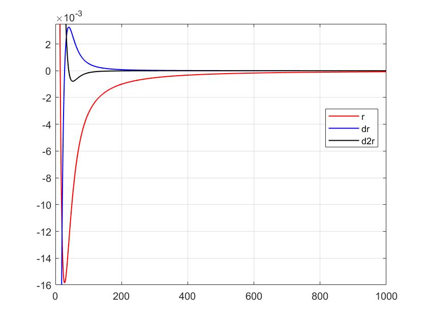
Figure 3.1: Graph of the covariance function $r(\cdot)$ of stationary fOU and its first two derivatives, e.g. $H=0.2$, $\sigma=\lambda=1$.

Lemma 3.1.

For the covariance function $r(\cdot)$ of stationary fOU process $X$ with $H<\frac{1}{2}$, we have the following properties:
(i) $r(t)$ is $2H$-Hölder continuous on $\mathbb{R}_{+}$, that is,

$$|r(t)-r(s)|\leq C_{H}|t-s|^{2H},$$

for any $s,t\in\mathbb{R}_{+}$ and $C_{H}$ depends on $H,\sigma,\lambda$ only (we may ignore $\sigma,\lambda$).
(ii) There exist constants $0<T_{0}<T_{1}$ such that $r^{\prime\prime}(T_{0})=0$, and $r^{\prime\prime}(t)>0$ on interval $(0,T_{0})$, $r^{\prime\prime}(t)<0$ on interval $(T_{1},\infty)$. That is, $r$ is convex on $[0,T_{0}]$ and concave on $(T_{1},\infty)$.

Proof.

For covariance function $r(\cdot)$, near $t=0$,

$$r(t)=\sigma^{2}\lambda^{-2H}HG(2H)\left(1-\frac{\lambda^{2H}}{G(2H+1)}t^{2H}+o(t^{2H})\right),$$

and for $t$ large enough (see Theorem 2.3, [9]),

$$r(t)=\frac{1}{2}\sigma^{2}\sum_{n=1}^{N}\lambda^{-2n}\left(\prod_{k=0}^{2n-1}(2H-k)\right)t^{2H-2n}+O(t^{2H-2N-2}).$$

Since $r(t)$ is continuous on $[0,\infty)$ and one can also see that $r(t)$ has polynomial decay to zero as $t$ large from above equality.

For (i), we have $\max_{t\geq 0}|r(t)|=C<\infty$, for any $s,t\in\mathbb{R}_{+}$ and $|t-s|\geq 1$, then

$$|r(t)-r(s)|\leq 2C\leq 2C|t-s|^{2H}.$$

For any $s,t\in\mathbb{R}_{+}$ and $|t-s|<1$, we show the statement in three case: $s,t\in[0,1]$, $s,t\in[1,\infty)$ and $0\leq s<1<t(<2)$. For the first and third terms, we actually need to show that for any $s,t\in[0,2]$ and $|t-s|<1$, there exists a constant $C$ such that $|r(t)-r(s)|\leq C|t-s|^{2H}.$ Since $r(t)=-ct^{2H}+\varphi(t)$, where $\varphi(\cdot)$ is smooth on $\mathbb{R}_{+}$, then

$$|r(t)-r(s)|\leq c|t-s|^{2H}+\max_{0\leq u\leq 2}|\varphi^{\prime}(u)||t-s|\leq C|t-s|^{2H}.$$

For the second case, i.e. for any $s,t\in[1,\infty)$ and $|t-s|<1$, we have

$$|r(t)-r(s)|\leq\max_{u\geq 1}|r^{\prime}(u)||t-s|\leq C|t-s|^{2H}.$$

Thus we proved the statement (i).

For (ii), one can see that there exists a small number $\varepsilon>0$ such that $r^{\prime\prime}(\varepsilon)>0$ and a large number $T_{1}>0$ such that, for all $t\geq T_{1}$, $r^{\prime\prime}(t)<0$. By the continuity of $r^{\prime\prime}$ on $(0,\infty)$, there exists a $T_{0}\in(\varepsilon,T_{1})$ satisfying $r^{\prime\prime}(T_{0})=0$ and $r^{\prime\prime}(t)>0$ for any $t\in(0,T_{0})$. ∎

Followings are important properties of fOU processes when $H<\frac{1}{2}$. It is well-known that, increments of fBM are negatively correlated when $H<\frac{1}{2}$, and positively correlated when $H>\frac{1}{2}$, while for $H=\frac{1}{2}$ increments over different time periods are independent. We found that for fOU process with $H<\frac{1}{2}$, the disjoint increments are locally negative correlated. If the distance of the intervals corresponding the disjoint increments is large, then they are positively correlated, we call it long-range positive correlation. See the theorem below. Heuristically, fOU process is locally like fBM so that it has the locally negative correlation property as fBM when $H<\frac{1}{2}$. For long distance the drift becomes the dominated force, so the fOU behaves positively correlated. In the case where $H=\frac{1}{2}$, the fOU is the standard OU process driven by standard Bownian motion. The properties of it are well known. Our main concern here is for the true fOU process case with $H<\frac{1}{2}$.

Theorem 3.2.

Consider the stationary fOU process $X$ with $H<\frac{1}{2}$. $T_{0},T_{1}$ are given in the previous lemma.
(i) (Locally negative correlation) For any $s_{0}$ and $s_{0}\leq t_{i}<t_{i+1}\leq t_{j}<t_{j+1}\leq s_{0}+T_{0}$, then

$$\mathbb{E}(X_{t_{i+1}}-X_{t_{i}})(X_{t_{j+1}}-X_{t_{j}})\leq 0.$$ (3.1)

(ii) (Long-range positive correlation) For any $0\leq t_{i}<t_{i+1}<t_{j}<t_{j+1}$, and if $t_{j}-t_{i+1}>T_{1}$, then

$$\mathbb{E}(X_{t_{i+1}}-X_{t_{i}})(X_{t_{j+1}}-X_{t_{j}})\geq 0.$$ (3.2)

Proof.

(i) Since

$$\begin{split}&\ \ \ \ \mathbb{E}(X_{t_{i+1}}-X_{t_{i}})(X_{t_{j+1}}-X_{t_{j}})\\ &=\left(r(t_{j+1}-t_{i+1})-r(t_{j+1}-t_{i})\right)-\left(r(t_{j}-t_{i+1})-r(t_{j}-t_{i})\right)\\ &=\left(r(x_{3})-r(x_{4})\right)-\left(r(x_{1})-r(x_{2})\right)\\ &=-\left[\left(r(x_{4})-r(x_{3})\right)-\left(r(x_{2})-r(x_{1})\right)\right],\end{split}$$

where $x_{1}:=t_{j}-t_{i+1}$, $x_{2}:=t_{j}-t_{i}$, $x_{3}:=t_{j+1}-t_{i+1}$, $x_{4}:=t_{j+1}-t_{i}$, then we have $0\leq x_{1}<x_{2}\leq x_{3}<x_{4}\leq T_{0}$ or $0\leq x_{1}<x_{3}\leq x_{2}<x_{4}\leq T_{0}$, and

$$\frac{r(x_{4})-r(x_{3})}{x_{4}-x_{3}}\geq\frac{r(x_{2})-r(x_{1})}{x_{2}-x_{1}},$$

by convexity of $r$. This proves (3.1).
(ii) The proof of (3.2) is almost the same as (i). ∎

Now we have the following propositions.

Proposition 3.3.

For the stationary fOU process $X$, it satisfies that

$$\mathbb{E}|X_{t}-X_{s}|^{2}\leq C_{H}|t-s|^{2H},$$ (3.3)

for any $s,t\in\mathbb{R}_{+}$, and $C_{H}$ depends on $H,\sigma,\lambda$ only (we ignore $\sigma,\lambda$ here).

Proof.

Since $X$ is a stationary Gaussian process, then

$$\begin{split}\mathbb{E}|X_{t}-X_{s}|^{2}&=\mathbb{E}(X_{t}^{2}+X_{s}^{2}-2X_{t}X_{s})\\ &=2(r(0)-r(|t-s|))\\ &\leq C_{H}|t-s|^{2H}.\end{split}$$

The last inequality holds by $2H$-Hölder continuity of the covariance function $r(t)$, i.e. Lemma 3.1.(i). ∎

Proposition 3.4.

Let $X$ be the stationary fOU process with $H\in(0,\frac{1}{2})$. Then its covariance $R_{X}(s,t)=\mathbb{E}(X_{s}X_{t})$ is of finite $\frac{1}{2H}$-variation on $[s_{0},s_{0}+T_{0}]^{2}$ in $2D$ sense for any $s_{0}$. Moreover, there exist constants $C=C(H)$ and $T_{0}>0$ such that, for all $s<t$ in $[s_{0},s_{0}+T_{0}]$,

$$|R_{X}|_{\frac{1}{2H}-var;[s,t]^{2}}\leq C(H)|t-s|^{2H},$$ (3.4)

where

$$|R_{X}|_{\rho-var;[s,t]^{2}}^{\rho}:=\sup\sum_{i,j}\left|\mathbb{E}\left[(X_{t_{i+1}}-X_{t_{i}})(X_{t^{\prime}_{j+1}}-X_{t^{\prime}_{j}})\right]\right|^{\rho},$$ (3.5)

and $\mathcal{P}=\{t_{i}\}$, $\mathcal{P}^{\prime}=\{t^{\prime}_{j}\}$ are any two partitions of interval $[s,t]$.

Proof.

By Lemma 5.54 of [16], we just need to show the finite $\frac{1}{2H}$-variation by the same partition $\mathcal{P}=\{t_{i}\}$ of interval $[s,t]\subset[s_{0},s_{0}+T_{0}]$. Let us consider

$$\sum_{i,j}\left|\mathbb{E}\left[(X_{t_{i+1}}-X_{t_{i}})(X_{t_{j+1}}-X_{t_{j}})\right]\right|^{\frac{1}{2H}}.$$ (3.6)

For a fixed $i$, and $i\neq j$, $\mathbb{E}\left[(X_{t_{i+1}}-X_{t_{i}})(X_{t_{j+1}}-X_{t_{j}})\right]\leq 0$ for $H<\frac{1}{2}$ by Theorem 3.2, hence,

$$\begin{split}&\ \ \ \ \sum_{j}\left|\mathbb{E}\left[X_{t_{i},t_{i+1}}X_{t_{j},t_{j+1}}\right]\right|^{\frac{1}{2H}}\\ &=\sum_{j\neq i}\left|\mathbb{E}\left[X_{t_{i},t_{i+1}}X_{t_{j},t_{j+1}}\right]\right|^{\frac{1}{2H}}+\left(\mathbb{E}\left|X_{t_{i},t_{i+1}}\right|^{2}\right)^{\frac{1}{2H}}\\ &\leq\left|\mathbb{E}\left(\sum_{j\neq i}X_{t_{i},t_{i+1}}X_{t_{j},t_{j+1}}\right)\right|^{\frac{1}{2H}}+\left(\mathbb{E}\left|X_{t_{i},t_{i+1}}\right|^{2}\right)^{\frac{1}{2H}}\\ &\leq\left(2^{\frac{1}{2H}-1}\left|\mathbb{E}\left(\sum_{j}X_{t_{i},t_{i+1}}X_{t_{j},t_{j+1}}\right)\right|^{\frac{1}{2H}}+2^{\frac{1}{2H}-1}\left(\mathbb{E}\left|X_{t_{i},t_{i+1}}\right|^{2}\right)^{\frac{1}{2H}}\right)\\ &\ \ \ \ +\left(\mathbb{E}\left|X_{t_{i},t_{i+1}}\right|^{2}\right)^{\frac{1}{2H}}\\ &\leq C(H)\left|\mathbb{E}\left[X_{t_{i},t_{i+1}}X_{s,t}\right]\right|^{\frac{1}{2H}}+C(H)\left(\mathbb{E}\left|X_{t_{i},t_{i+1}}\right|^{2}\right)^{\frac{1}{2H}}.\end{split}$$

Therefore, we have

$$\sum_{i,j}\left|\mathbb{E}\left[X_{t_{i},t_{i+1}}X_{t_{j},t_{j+1}}\right]\right|^{\frac{1}{2H}}\leq C(H)\sum_{i}\left|\mathbb{E}\left[X_{t_{i},t_{i+1}}X_{s,t}\right]\right|^{\frac{1}{2H}}+C(H)\sum_{i}\left(\mathbb{E}\left|X_{t_{i},t_{i+1}}\right|^{2}\right)^{\frac{1}{2H}}.$$

The second term on the right hand side is controlled by $C(H)|t-s|$ by Proposition 3.3. Now we show that

$$\sum_{i}\left|\mathbb{E}\left[X_{t_{i},t_{i+1}}X_{s,t}\right]\right|^{\frac{1}{2H}}\leq C(H)|t-s|.$$

Since

$$\begin{split}\left|\mathbb{E}\left[X_{t_{i},t_{i+1}}X_{s,t}\right]\right|&=\left|\mathbb{E}\left(X_{t_{i+1}}X_{t}-X_{t_{i}}X_{t}+X_{t_{i}}X_{s}-X_{t_{i+1}}X_{s}\right)\right|\\ &=\left|r(t-t_{i+1})-r(t-t_{i})+r(t_{i}-s)-r(t_{i+1}-s)\right|\\ &\leq\left|r(t-t_{i+1})-r(t-t_{i})\right|+\left|r(t_{i}-s)-r(t_{i+1}-s)\right|\\ &\leq C_{H}\left|t_{i+1}-t_{i}\right|^{2H}+C_{H}\left|t_{i+1}-t_{i}\right|^{2H}\leq 2C_{H}\left|t_{i+1}-t_{i}\right|^{2H},\end{split}$$

thus

$$\sum_{i}\left|\mathbb{E}\left[X_{t_{i},t_{i+1}}X_{s,t}\right]\right|^{\frac{1}{2H}}\leq\sum_{i}C(H)\left|t_{i+1}-t_{i}\right|\leq C(H)|t-s|.$$

Now we have completed the proof. ∎

Corollary 3.5.

Let $X$ be the stationary fOU process with $H\in(0,\frac{1}{2})$. Then its covariance $R_{X}(s,t)=\mathbb{E}(X_{s}X_{t})$ is of finite $\frac{1}{2H}$-variation on $[0,T]^{2}$ in $2D$ sense. Moreover, there exists a constant $C=C(H)$ such that, for all $s<t$ in $[0,T]$,

$$|R_{X}|_{\frac{1}{2H}-var;[s,t]^{2}}^{\frac{1}{2H}}\leq C(H)|t-s|.$$ (3.7)

Proof.

We divide the interval $[0,T]$ into $m+1=\left[\frac{T}{T_{0}}\right]+1$ pieces, denote them as $[0,T_{0}]$, $[T_{0},2T_{0}]$, $\cdots$, $[(m-1)T_{0},mT_{0}]$, $[mT_{0},T]$. For any subinterval $[s,t]\subset[0,T]$, there exist $q_{1},q_{2}\in\mathbb{N}$ such that $s\in[(q_{1}-1)T_{0},q_{1}T_{0}]$ and $t\in[q_{2}T_{0},(q_{2}+1)T_{0}]$, by the subadditivity of $|R_{X}|_{\frac{1}{2H}-var;[\cdot,\cdot]^{2}}^{\frac{1}{2H}}$, then we have

$$\begin{split}|R_{X}|_{\frac{1}{2H}-var;[s,t]^{2}}^{\frac{1}{2H}}&\leq|R_{X}|_{\frac{1}{2H}-var;[s,q_{1}T_{0}]^{2}}^{\frac{1}{2H}}+|R_{X}|_{\frac{1}{2H}-var;[q_{1}T_{0},(q_{1}+1)T_{0}]^{2}}^{\frac{1}{2H}}+\cdots+|R_{X}|_{\frac{1}{2H}-var;[q_{2}T_{0},t]^{2}}^{\frac{1}{2H}}\\ &\leq C(H)(|q_{1}T_{0}-s|+|2q_{1}T_{0}-q_{1}T_{0}|+\cdots+|t-q_{2}T_{0}|)\\ &\leq C(H)|t-s|.\end{split}$$

This completes the proof of the corollary. ∎

3.1.2 Regularity of fOU processes

In the following, we study the $\alpha$-Hölder continuity of one dimensional, stationary fOU process $X_{t}=\sigma\int_{-\infty}^{t}e^{-\lambda(t-s)}dB_{s}^{H}$. Before showing the regularity, we recall the usual Garsia-Rodemich-Rumsey inequality (see e.g., page 60, Stroock and Varadhan [37]).

Lemma 3.6.

(Garsia-Rodemich-Rumsey inequality) Let $p(\cdot)$ and $\Psi(\cdot)$ be continuous, strictly increasing functions on $[0,\infty)$ such that

$$p(0)=\Psi(0)=0,\ \ \text{and}\ \ \lim_{t\to\infty}\Psi(t)=\infty.$$

Given $T>0$ and $\phi\in C([0,T],\mathbb{R}^{d})$, if there is a constant $B$ such that

$$\int_{0}^{T}\int_{0}^{T}\Psi\left(\frac{|\phi(t)-\phi(s)|}{p(|t-s|)}\right)dsdt\leq B,$$ (3.8)

then for all $0\leq s\leq t\leq T$,

$$|\phi(t)-\phi(s)|\leq 8\int_{0}^{|t-s|}\Psi^{-1}\left(\frac{4B}{u^{2}}\right)p(du).$$ (3.9)

As an application of this lemma above, we have

Proposition 3.7.

Let $X$ be a one dimensional, stationary fOU process with $H\in(0,\frac{1}{2})$ on $[0,T]$. Then there exist a constant $0<\beta<1$ and an almost surely finite random variable $C$ independent of $T$ such that

$$|X_{t}-X_{s}|\leq CT^{\beta}|t-s|^{\alpha},\ a.s.$$ (3.10)

for any $\alpha\in(0,H)$, any $0\leq s,t\leq T$.

Proof.

By Proposition 3.3, we know that

$$\mathbb{E}|X_{t}-X_{s}|^{2}\leq C_{H}|t-s|^{2H}.$$ (3.11)

Since $X_{t}$ is Gaussian process, all the norms are equivalent, we get

$$\mathbb{E}|X_{t}-X_{s}|^{p}\leq C_{p}(\mathbb{E}|X_{t}-X_{s}|^{2})^{\frac{p}{2}}\leq C_{p,H}|t-s|^{pH},$$ (3.12)

for any $p>2$.

Next, we apply the Garsia-Rodemich-Rumsey inequality. Take $\Psi(x)=x^{p}$ and $p(x)=x^{H}$. Then inequality (3.12) implies that

$$\mathbb{E}\left(\int_{0}^{T}\int_{0}^{T}\Psi\left(\frac{|X_{t}-X_{s}|}{p(|t-s|)}\right)dsdt\right)\leq C_{p,H}T^{2}.$$

Define

$$B_{T}:=\int_{0}^{T}\int_{0}^{T}\Psi\left(\frac{|X_{t}-X_{s}|}{p(|t-s|)}\right)dsdt=\int_{0}^{T}\int_{0}^{T}\frac{|X_{t}-X_{s}|^{p}}{|t-s|^{pH}}dsdt.$$

Then for any $q>3$, we get

$$\mathbb{E}\left(\sum_{n=1}^{\infty}\frac{B_{n}}{n^{q}}\right)=\sum_{n=1}^{\infty}\frac{\mathbb{E}(B_{n})}{n^{q}}\leq\sum_{n=1}^{\infty}\frac{Cn^{2}}{n^{q}}<\infty.$$

Thus there exists an almost surely finite random variable $R$ independent of $n$ such that

$$\sum_{n=1}^{\infty}\frac{B_{n}}{n^{q}}\leq R,\ a.s.$$

So we have

$$B_{n}\leq Rn^{q},\ a.s.\ \ \ \forall n\geq 1,\ q>3.$$

Take $n=[T]$, then

$$B_{T}\leq B_{n+1}\leq R(n+1)^{q}\leq CRT^{q},\ a.s.\ \ \ \forall T>0,\ q>3.$$

Then the Garsia-Rodemich-Rumsey inequality gives that

$$\begin{split}\left|X_{t}-X_{s}\right|&\leq 8\int_{0}^{|t-s|}\Psi^{-1}\left(\frac{4B_{T}}{u^{2}}\right)p(du)\\ &\leq C(4B_{T})^{\frac{1}{p}}|t-s|^{H-2/p}\leq CR^{\frac{1}{p}}T^{\frac{q}{p}}|t-s|^{\alpha},\end{split}$$

for any $\alpha\in(0,H)$, $p>3\vee\left[\frac{2}{H-\alpha}\right]$ and $3<q<p$. This concludes the lemma. ∎

Remark 3.8.

When $X_{t}=\sigma\int_{0}^{t}e^{-\lambda(t-s)}dB_{s}^{H}$, it still satisfies inequality (3.10).

Besides, we prove a proposition for a function of fOU processes, which will be applied in section 5.

Proposition 3.9.

Let $B^{H}=(B^{H,1},B^{H,2},\cdots,B^{H,d})$ be a $d$-dimensional fBM with $H\in(0,\frac{1}{2})$, $X=(X^{1},X^{2},\cdots,X^{d})$ a $d$-dimensional fOU process, where $X_{t}^{i}=\sigma\int_{0}^{t}e^{-\lambda_{i}(t-s)}dB_{s}^{H,i}$, $\lambda_{i}>0$, $\sigma\in\mathbb{R}$. Define $F(X_{t}):=X_{t}\otimes X_{t}=(X_{t}^{i}X_{t}^{j})_{i,j=1,2,\cdots,d}$, and the norm of matrix $A$ as $\|A\|=\sum_{i,j=1}^{d}|a_{ij}|$. Then there exist a constant $0<\beta<1$, an almost surely finite random variable $C$ (independent of $T$) and a random variable $R_{T}$ (tends to zero almost surely as $T\to\infty$) such that

$$\sup_{s\neq t}\frac{\left\|F(X_{t})-F(X_{s})\right\|}{|t-s|^{\alpha}}\leq CR_{T}T^{\beta},$$ (3.13)

for any $0\leq s,t\leq T$, any $\alpha\in(0,H)$.

Proof.

First, we present a fact about supremum of one dimensional, stationary fOU process $(\overline{X}^{i})_{t}^{*}=\sup_{0\leq s\leq t}|\overline{X}_{s}^{i}|$ below. Since we know that $\overline{X}^{i}$ and $-\overline{X}^{i}$ have the same distribution and their covariance function is

$$r_{i}(t)=\mathrm{Cov}(\overline{X}_{s+t}^{i},\overline{X}_{s}^{i})=C\left(1-\frac{\lambda_{i}^{2H}}{G(2H+1)}t^{2H}+o(t^{2H})\right),$$ (3.14)

for $t$ small, where $C=\sigma^{2}\lambda_{i}^{-2H}HG(2H)$ and $G(\cdot)$ is Gamma function. So by Theorem 3.1 of Pickands [32], we know that for $t$ tending to infinity

$$\frac{1}{t^{\delta}}\sup_{0\leq s\leq t}\overline{X}_{s}^{i}\to 0,\ a.s.,\ \ \frac{1}{t^{\delta}}\sup_{0\leq s\leq t}(-\overline{X}_{s}^{i})\to 0,\ a.s.,$$

for any $\delta>0$. Since $(\overline{X}^{i})_{t}^{*}=(\sup_{0\leq s\leq t}\overline{X}_{s}^{i})\vee(\sup_{0\leq s\leq t}(-\overline{X}_{s}^{i}))$, then

$$\frac{(\overline{X}^{i})_{t}^{*}}{t^{\delta}}\to 0,\ a.s.$$ (3.15)

Since $X_{t}^{i}=\overline{X}_{t}^{i}-e^{-\lambda t}\overline{X}_{0}^{i}$, so we also have $\frac{(X^{i})_{t}^{*}}{t^{\delta}}\to 0,\ a.s$, where $(X^{i})_{t}^{*}=\sup_{0\leq s\leq t}|X_{s}^{i}|$.

Now define $R_{t}=\sup_{i=1,\cdots,d}\frac{(X^{i})_{t}^{*}}{t^{\delta}}$, then $R_{t}\to 0,\ a.s.$ as $t\to\infty$. For any $i,j=1,2,\cdots,d$, and $0\leq s,t\leq T$,

$$\begin{split}|X_{t}^{i}X_{t}^{j}-X_{s}^{i}X_{s}^{j}|&=|(X_{t}^{i}-X_{s}^{i})X_{t}^{j}+X_{s}^{i}(X_{t}^{j}-X_{s}^{j})|\\ &\leq|X_{t}^{j}||X_{t}^{i}-X_{s}^{i}|+|X_{s}^{i}||X_{t}^{j}-X_{s}^{j}|\\ &\leq(X^{j})_{T}^{*}|X_{t}^{i}-X_{s}^{i}|+(X^{i})_{T}^{*}|X_{t}^{j}-X_{s}^{j}|\\ &\leq CR_{T}T^{\delta}T^{\beta}|t-s|^{\alpha}+CR_{T}T^{\delta}T^{\beta}|t-s|^{\alpha}\\ &\leq CR_{T}T^{\delta+\beta}|t-s|^{\alpha},\end{split}$$

where the last second inequality is followed from Proposition 3.7. One can choose $\delta,\beta$ such that $0<\delta+\beta=:\beta^{\prime}<1$. Thus, we have . This completes the proof of the statement. ∎

3.1.3 Lévy area of multi-dimensional fOU processes

In this subsection, let $B^{H}=(B^{H,1},B^{H,2},\cdots,B^{H,d})$ be a $d$-dimensional fBM with $H\in(\frac{1}{3},\frac{1}{2})$, $X=(X^{1},X^{2},\cdots,X^{d})$ a $d$-dimensional fOU process, where $X_{t}^{i}=\sigma\int_{-\infty}^{t}e^{-\lambda_{i}(t-s)}dB_{s}^{H,i}$, $\lambda_{i}>0$, $\sigma\in\mathbb{R}$. Then $X=(X^{1},X^{2},\cdots,X^{d})$ is stationary (see [9]). Its covariance function is given by

$$R_{X}(s,t)=\mathrm{diag}(R_{1}(s,t),\cdots,R_{d}(s,t)),$$

where $R_{i}(s,t)=\mathbb{E}(X_{s}^{i}X_{t}^{i})$.

In this subsection, we will show one estimate for off-diagonal elements of Lévy area $\int_{0}^{t}X_{u}^{i}\circ d_{\mathfrak{R}_{1}}\mathbf{X}^{j}$ of the multi-dimensional fOU process $X$. We denote Stratonovich’s Lévy area of fOU process $X$ as

$$A(t):=\int_{0}^{t}X_{u}\circ d_{\mathfrak{R}_{1}}\mathbf{X}=\left(\int_{0}^{t}X_{u}^{i}\circ d_{\mathfrak{R}_{1}}\mathbf{X}^{j}\right)_{i,j=1,2,\cdots,d},$$

and $A_{ij}(t)$ as its components.

Before showing the estimate of off-diagonal elements, we recall a lemma based on Wiener chaos. We denote $\mathcal{H}_{n}(\mathbb{P})$ as homogeneous Wiener chaos of order $n$ and $\mathcal{C}^{n}(\mathbb{P}):=\oplus_{j=0}^{n}\mathcal{H}_{j}(\mathbb{P})$ the Wiener chaos (or non-homogeneous chaos) of order $n$. The lemma below gives the hypercontractivity of Wiener chaos.

Lemma 3.10.

(Refer to, e.g., Lemma 15.21, [16]) Let $q\in\mathbb{N}$ and $Z\in\mathcal{C}^{q}(\mathbb{P})$. Then, for $p>2$,

$$(\mathbb{E}|Z|^{2})^{\frac{1}{2}}\leq(\mathbb{E}|Z|^{p})^{\frac{1}{p}}\leq(q+1)(p-1)^{\frac{q}{2}}(\mathbb{E}|Z|^{2})^{\frac{1}{2}}.$$ (3.16)

Now we illustrate one estimate for off-diagonal elements, i.e. when $i\neq j$, we have the following proposition.

Proposition 3.11.

Let $X=(X^{1},\cdots,X^{d})$ be a $d$-dimensional, stationary fOU process with $H\in(\frac{1}{3},\frac{1}{2})$, and $A_{ij}(t)=\int_{0}^{t}X_{u}^{i}\circ d_{\mathfrak{R}_{1}}\mathbf{X}^{j},i\neq j$, be the off-diagonal elements of Stratonovich’s Lévy area of $X$. Then there exist $0<\beta<1$ and an almost surely finite random variable $\widetilde{C}$ such that

$$|A_{ij}(t)-A_{ij}(s)|\leq\widetilde{C}n^{\beta},\ a.s.$$ (3.17)

for any $s,t\in[n-1,n]$ and any integer $n\geq 1$.

Proof.

First, we rewrite $R_{i}(s,t)$ as

$$R_{i}\binom{\ s\ }{\ t\ }=\mathbb{E}X_{s}^{i}X_{t}^{i},$$

and denote

$$R_{i}\binom{s}{u,v}=\mathbb{E}X_{s}^{i}X_{u,v}^{i},\ R_{i}\binom{s,t}{u}=\mathbb{E}X_{s,t}^{i}X_{u}^{i},\ R_{i}\binom{s,t}{u,v}=\mathbb{E}X_{s,t}^{i}X_{u,v}^{i}.$$

For the second moment of the Lévy area,

$$\begin{split}\mathbb{E}\left(\left|\int_{s}^{t}X_{u}^{i}\circ d_{\mathfrak{R}_{1}}\mathbf{X}^{j}\right|^{2}\right)&=\mathbb{E}\left(\int_{s}^{t}\int_{s}^{t}X_{u}^{i}X_{v}^{i}\circ d_{\mathfrak{R}_{1}}\mathbf{X}^{j}\circ d_{\mathfrak{R}_{1}}\mathbf{X}^{j}\right)\\ &=\int_{s}^{t}\int_{s}^{t}\mathbb{E}(X_{u}^{i}X_{v}^{i})d\mathbb{E}(X_{u}^{j}X_{v}^{j})\\ &=\int_{s}^{t}\int_{s}^{t}R_{i}\binom{\ u\ }{\ v\ }dR_{j}\binom{\ u\ }{\ v\ },\end{split}$$

where the integral which appears on the right hand side above can be viewed as a 2-dimensional (2D) Young’s integral (see e.g. Section 6.4 of Friz and Victoir [16]). Then we have

$$\begin{split}\int_{s}^{t}\int_{s}^{t}R_{i}\binom{\ u\ }{\ v\ }dR_{j}\binom{\ u\ }{\ v\ }&=\int_{s}^{t}\int_{s}^{t}R_{i}\binom{s,u}{s,v}dR_{j}\binom{\ u\ }{\ v\ }+\int_{s}^{t}\int_{s}^{t}R_{i}\binom{s,u}{s}dR_{j}\binom{\ u\ }{\ v\ }\\ &\ \ \ +\int_{s}^{t}\int_{s}^{t}R_{i}\binom{s}{s,v}dR_{j}\binom{\ u\ }{\ v\ }+R_{i}\binom{\ s\ }{\ s\ }\int_{s}^{t}\int_{s}^{t}dR_{j}\binom{\ u\ }{\ v\ }\\ &=:I+II+III+IV.\end{split}$$

For the first term $I$, by Young-Lóeve-Towghi inequality (see e.g. Theorem 6.18 of [16]), we have

$$\begin{split}I&\leq C|R_{i}|_{\frac{1}{2H}-var;[s,t]^{2}}|R_{j}|_{\frac{1}{2H}-var;[s,t]^{2}}\\ &\leq C\max\{|R_{i}|_{\frac{1}{2H}-var;[s,t]^{2}}^{2},|R_{j}|_{\frac{1}{2H}-var;[s,t]^{2}}^{2}\}.\end{split}$$

Then by Corollary 3.5, we have that

$$I=\int_{s}^{t}\int_{s}^{t}R_{i}\binom{s,u}{s,v}dR_{j}\binom{\ u\ }{\ v\ }\leq C|t-s|^{4H}.$$ (3.18)

For the second term $II$, by Young 1D estimate (see e.g. Theorem 6.8 of [16]), we have

$$\begin{split}II&=\int_{s}^{t}R_{i}\binom{s,u}{s}dR_{j}\binom{u}{s,t}\\ &\leq C\left|R_{i}\binom{\ \cdot\ }{\ s\ }\right|_{\frac{1}{2H}-var;[s,t]}\left|R_{j}\binom{\cdot}{s,t}\right|_{\frac{1}{2H}-var;[s,t]},\end{split}$$

where

$$\begin{split}\left|R_{i}\binom{\ \cdot\ }{\ s\ }\right|_{\frac{1}{2H}-var;[s,t]}^{\frac{1}{2H}}&=\sup_{\mathcal{P}}\sum_{\ell}\left|R_{i}\binom{\ t_{\ell+1}\ }{\ s\ }-R_{i}\binom{\ t_{\ell}\ }{\ s\ }\right|^{\frac{1}{2H}}\\ &=\sup_{\mathcal{P}}\sum_{\ell}\left|r_{i}(t_{\ell+1}-s)-r_{i}(t_{\ell}-s)\right|^{\frac{1}{2H}}\\ &\leq\sup_{\mathcal{P}}\sum_{\ell}C_{H}\left|t_{\ell+1}-t_{\ell}\right|\leq C_{H}|t-s|,\end{split}$$

and

$$\begin{split}\left|R_{j}\binom{\cdot}{s,t}\right|_{\frac{1}{2H}-var;[s,t]}^{\frac{1}{2H}}&=\sup_{\mathcal{P}}\sum_{\ell}\left|R_{j}\binom{\ t_{\ell+1}\ }{s,t}-R_{j}\binom{\ t_{\ell}\ }{s,t}\right|^{\frac{1}{2H}}\\ &=\sup_{\mathcal{P}}\sum_{\ell}\left|\mathbb{E}(X_{t_{\ell},t_{\ell+1}}^{j}X_{s,t}^{j})\right|^{\frac{1}{2H}}\leq\left|R_{j}\right|_{\frac{1}{2H}-var;[s,t]^{2}}^{\frac{1}{2H}}.\end{split}$$

In above estimate, function $r_{i}$ is the covariance $r_{i}(t)=\mathbb{E}(X_{s}^{i}X_{s+t}^{i})$. Thus, we have

$$II=\int_{s}^{t}\int_{s}^{t}R_{i}\binom{s,u}{s}dR_{j}\binom{\ u\ }{\ v\ }\leq C|t-s|^{4H}.$$ (3.19)

For the third term $III$, it is the same with the second term $II$ line by line. So

$$III=\int_{s}^{t}\int_{s}^{t}R_{i}\binom{s}{s,v}dR_{j}\binom{\ u\ }{\ v\ }\leq C|t-s|^{4H}.$$ (3.20)

For the last term $IV$,

$$\begin{split}IV&=R_{i}\binom{\ s\ }{\ s\ }\left(R_{j}\binom{\ t\ }{\ t\ }-R_{j}\binom{\ s\ }{\ t\ }-R_{j}\binom{\ t\ }{\ s\ }+R_{j}\binom{\ s\ }{\ s\ }\right)\\ &=r_{i}(0)(2r_{j}(0)-2r_{j}(t-s))\leq C|t-s|^{2H}.\end{split}$$ (3.21)

Now combing inequalities (3.18),(3.19),(3.20) and (3.21), we get

$$\mathbb{E}\left(\left|\int_{s}^{t}X_{u}^{i}\circ d_{\mathfrak{R}_{1}}\mathbf{X}^{j}\right|^{2}\right)\leq C|t-s|^{4H}+C|t-s|^{2H}.$$ (3.22)

Let $s<t$ and $s,t\in[n-1,n]$, so we have

$$\mathbb{E}\left(\left|\int_{s}^{t}X_{u}^{i}\circ d_{\mathfrak{R}_{1}}\mathbf{X}^{j}\right|^{2}\right)\leq C|t-s|^{2H}.$$

Now we turn to prove the estimate, for arbitrary $p\geq 2$, by the hypercontractivity of Wiener chaos (see Lemma 3.10), we further have

$$\begin{split}\mathbb{E}[|A_{ij}(t)-A_{ij}(s)|^{p}]&=\mathbb{E}\left(\left|\int_{s}^{t}X_{u}^{i}\circ d_{\mathfrak{R}_{1}}\mathbf{X}^{j}\right|^{p}\right)\\ &\leq 3^{p}(p-1)^{p}\left(\mathbb{E}\left|\int_{s}^{t}X_{u}^{i}\circ d_{\mathfrak{R}_{1}}\mathbf{X}^{j}\right|^{2}\right)^{\frac{p}{2}}\\ &\leq C|t-s|^{pH}.\end{split}$$

Take $\Psi(x)=x^{p}$ and $p(x)=x^{H}$, the above inequality implies that

$$\mathbb{E}\left(\int_{n}^{n+1}\int_{n}^{n+1}\Psi\left(\frac{|A_{ij}(t)-A_{ij}(s)|}{p(|t-s|)}\right)dsdt\right)\leq C.$$

Define

$$B_{n}:=\int_{n}^{n+1}\int_{n}^{n+1}\Psi\left(\frac{|A_{ij}(t)-A_{ij}(s)|}{p(|t-s|)}\right)dsdt=\int_{n}^{n+1}\int_{n}^{n+1}\frac{|A_{ij}(t)-A_{ij}(s)|^{p}}{|t-s|^{pH}}dsdt.$$

Then for any $q>1$, we get

$$\mathbb{E}\left(\sum_{n=1}^{\infty}\frac{B_{n}}{n^{q}}\right)=\sum_{n=1}^{\infty}\frac{\mathbb{E}(B_{n})}{n^{q}}\leq\sum_{n=1}^{\infty}\frac{C}{n^{q}}<\infty.$$

Thus there exists an almost surely finite random variable $R$ independent of $n$ such that

$$\sum_{n=1}^{\infty}\frac{B_{n}}{n^{q}}\leq R,\ a.s.$$

So we have

$$B_{n}\leq Rn^{q},\ a.s.\ \ \ \forall n\geq 1,\ q>1.$$ (3.23)

Apply the Garsia-Rodemich-Rumsey inequality, and for any $n-1\leq s<t\leq n$, we get

$$\begin{split}\left|A_{ij}(t)-A_{ij}(s)\right|&\leq 8\int_{0}^{|t-s|}\Psi^{-1}\left(\frac{4B_{n}}{u^{2}}\right)p(du)\leq 8H\int_{0}^{1}\left(\frac{4B_{n}}{u^{2}}\right)^{\frac{1}{p}}u^{H-1}du\\ &=\frac{8H}{H-2/p}(4B_{n})^{\frac{1}{p}}\leq CR^{\frac{1}{p}}n^{\frac{q}{p}},\ \ \ a.s.\end{split}$$

for any $p>\frac{2}{H}$ and $1<q<p$. Thus we complete this proof. ∎

3.2 Long time asymptotic of Lévy area

Now in this subsection, we consider the multi-dimensional fOU process which is the solution to stochastic differential equation

$$dX_{t}=-\Gamma X_{t}dt+\sigma dB_{t}^{H},\ X_{0}=0,$$ (3.24)

where $\Gamma$ is a symmetric, positive-definite matrix, $\sigma$ is a constant, and $B^{H}=(B^{H,1},B^{H,2},\cdots,B^{H,d})$ is a $d$-dimensional fBM. Our aim in this section is to show a long time asymptotic property of Lévy area $A(t)=\int_{0}^{t}X_{s}\circ d_{\mathfrak{R}_{1}}\mathbf{X}$ of fOU processes $X$. That is to show

$$\frac{1}{t}A(t)=\frac{1}{t}\int_{0}^{t}X_{s}\circ d_{\mathfrak{R}_{1}}\mathbf{X}\to 0,\ a.s.$$

as $t$ goes to infinity.

The components of solution process $X$ are not independent since the interactions between each other. We first make an orthogonal transformation for this dynamical system. Since the drift matrix $\Gamma$ is symmetric and positive-definite, there exists an orthogonal matrix $\overline{\Sigma}$ such that

$$\overline{\Sigma}\Gamma\overline{\Sigma}^{T}=\Lambda,$$ (3.25)

where $\Lambda=\mathrm{diag}\{\lambda_{1},\cdots,\lambda_{d}\}$ and $0<\lambda_{1}\leq\cdots\leq\lambda_{d}$.

Define $\widetilde{X}_{t}:=\overline{\Sigma}X_{t}$, and $\widetilde{B}_{t}^{H}:=\overline{\Sigma}B_{t}^{H}$, since $\overline{\Sigma}$ is an orthogonal matrix, $\widetilde{B}_{t}^{H}$ is still a $d$-dimensional fBM with Hurst parameter $H$. Then stochastic differential equation (3.24) becomes

$$d\widetilde{X}_{t}=-\Lambda\widetilde{X}_{t}dt+\sigma d\widetilde{B}_{t}^{H}.$$ (3.26)

Now the fOU process $\widetilde{X}_{t}$ has independent components. We also have that

$$\int_{0}^{t}X_{s}\circ d_{\mathfrak{R}_{1}}\mathbf{X}=\overline{\Sigma}^{T}\left(\int_{0}^{t}\widetilde{X}_{s}\circ d_{\mathfrak{R}_{1}}\mathbf{\widetilde{X}}\right)\overline{\Sigma}.$$

What we should prove now is that

$$\frac{1}{t}\int_{0}^{t}\widetilde{X}_{s}\circ d_{\mathfrak{R}_{1}}\mathbf{\widetilde{X}}\to 0,\ a.s.$$

as $t$ goes to infinity.

We may ignore the symbol tilde and use $X,B^{H}$ to denote $\widetilde{X}$ and $\widetilde{B}^{H}$, respectively, for simplicity. Now the $d$-dimensional fOU process $X=(X^{1},X^{2},\cdots,X^{d})$ has independent components and satisfies

$$X_{t}^{i}=\sigma\int_{0}^{t}e^{-\lambda_{i}(t-s)}dB_{s}^{H,i},\ i=1,2,\cdots,d.$$ (3.27)

Define

$$\overline{X}_{t}^{i}=\sigma\int_{-\infty}^{t}e^{-\lambda_{i}(t-s)}dB_{s}^{H,i},\ i=1,2,\cdots,d.$$ (3.28)

Then $\{\overline{X}_{t}^{i},t\geq 0\}$ are stationary, ergodic, Gaussian processes, see [9].

3.2.1 On-diagonal case

Lemma 3.12.

For the on-diagonal components of Lévy area $A(t)=\int_{0}^{t}X_{s}\circ d_{\mathfrak{R}_{1}}\mathbf{X}$, we have

$$\frac{1}{t}A_{ii}(t)=\frac{1}{t}\int_{0}^{t}X_{s}^{i}\circ d_{\mathfrak{R}_{1}}\mathbf{X}^{i}\to 0,\ a.s.,\ \forall\ i=1,2,\cdots,d.$$ (3.29)

as $t$ tends to infinity.

Proof.

First, we show that for any $\alpha>0$,

$$\lim_{t\to\infty}\frac{\overline{X}_{t}^{i}}{t^{\alpha}}=0,\ a.s.$$ (3.30)

As we know that the covariance of the process $\overline{X}_{t}^{i}$ is

$$r_{i}(t)=\mathrm{Cov}(\overline{X}_{s+t}^{i},\overline{X}_{s}^{i})=C\left(1-\frac{\lambda_{i}^{2H}}{G(2H+1)}t^{2H}+o(t^{2H})\right),$$ (3.31)

for $t$ small, where $C=\sigma^{2}\lambda_{i}^{-2H}HG(2H)$ and $G(\cdot)$ is Gamma function. Then the limit (3.30) follows from Theorem 3.1 of Pickands [32].

Since $X_{t}^{i}=\overline{X}_{t}^{i}-e^{-\lambda_{i}t}\overline{X}_{0}^{i}$ and

$$\int_{0}^{t}X_{s}^{i}\circ d_{\mathfrak{R}_{1}}\mathbf{X}^{i}=\frac{1}{2}(X_{t}^{i})^{2},$$

then from (3.30), it follows that

$$\lim_{t\to\infty}\frac{1}{t}\int_{0}^{t}X_{s}^{i}\circ d_{\mathfrak{R}_{1}}\mathbf{X}^{i}=0,\ a.s.$$

Thus, we conclude this lemma for on-diagonal case. ∎

3.2.2 Off-diagonal case

Let $X=(X^{1},X^{2},\cdots,X^{d})$ be the $d$-dimensional, stationary Gaussian process given by (3.28). Its covariance function is given by

$$R_{X}(s,t)=\mathrm{diag}(R_{1}(s,t),\cdots,R_{d}(s,t)),$$

where $R_{i}(s,t):=\mathbb{E}(X_{s}^{i}X_{t}^{i})$.

When $i\neq j$, we have (as proof of equation (3.22) in Proposition 3.11) that

$$\mathbb{E}\left(\left|\int_{0}^{t}X_{s}^{i}\circ d_{\mathfrak{R}_{1}}\mathbf{X}^{j}\right|^{2}\right)\leq Ct^{4H}+Ct^{2H}.$$ (3.32)

When $t\geq 1$, we have

$$\mathbb{E}\left(\left|\int_{0}^{t}X_{s}^{i}\circ d_{\mathfrak{R}_{1}}\mathbf{X}^{j}\right|^{2}\right)\leq Ct^{4H}.$$ (3.33)

Now we define $A_{ij}(t)=\int_{0}^{t}X_{s}^{i}\circ d_{\mathfrak{R}_{1}}\mathbf{X}^{j}$ as in subsection 3.1.3, and $Z_{n}^{ij}:=n^{-2H}A_{ij}(n)$ we first show that when $t=n\in\mathbb{N}$ (discrete sequence), we have

$$\lim_{n\to\infty}\frac{1}{n}A_{ij}(n)=0,\ a.s.$$ (3.34)

Proposition 3.13.

For the discrete sequence $\{\frac{1}{n}A_{ij}(n),n\geq 1\}$ and $H\in(\frac{1}{3},\frac{1}{2})$, we have

$$\frac{1}{n}A_{ij}(n)\to 0,\ a.s.$$ (3.35)

as $n$ goes to infinity.

Proof.

By the inequality (3.33), we have

$$\mathbb{E}|A_{ij}(n)|^{2}\leq Cn^{4H}.$$

Then

$$\sup_{n}\mathbb{E}|Z_{n}^{ij}|^{2}\leq C.$$

According Proposition 15.20 of [16], we know that $Z_{n}^{ij}$ belongs to the second Wiener chaos $\mathcal{C}^{2}(\mathbb{P})$. By Lemma 3.10, we have

$$\sup_{n}\mathbb{E}|Z_{n}^{ij}|^{p}\leq 3^{p}(p-1)^{p}\sup_{n}(\mathbb{E}|Z_{n}^{ij}|^{2})^{\frac{p}{2}}<\infty.$$

For any $\epsilon>0$, by Chebyshev inequality, we have

$$\mathbb{P}\left(|A_{ij}(n)|>n\epsilon\right)=\mathbb{P}\left(|Z_{n}^{ij}|>n^{1-2H}\epsilon\right)\leq\frac{1}{n^{p(1-2H)}\epsilon^{p}}\sup_{n}\mathbb{E}|Z_{n}^{ij}|^{p}$$

where $p>\frac{1}{1-2H}$.

Then,

$$\sum_{n}\mathbb{P}\left(|A_{ij}(n)|>n\epsilon\right)\leq\sum_{n}\frac{C}{n^{p(1-2H)}\epsilon^{p}}<\infty.$$

The almost sure convergence follows from the Borel-Cantelli lemma. ∎

Now we can conclude this subsection, that is, to show the limit for arbitrary $t$ rather than at discrete time $\mathbb{N}_{+}$.

Theorem 3.14.

Suppose stochastic process $X_{t}$ is fOU process which is the solution to stochastic differential equation (3.24) and $\Gamma$ is symmetric and positive-definite. Then

$$\frac{1}{t}A(t)=\frac{1}{t}\int_{0}^{t}X_{s}\otimes\circ d_{\mathfrak{R}_{1}}\mathbf{X}\to 0,\ a.s.,$$

as $t\to\infty$, where the above integral is in Stratonovich sense.

Proof.

First, assume that $X$ is the stationary fOU process as in equation (3.28). The on-diagonal case is proved in Lemma 3.12. For the off-diagonal case, since

$$\frac{1}{t}|A_{ij}(t)|\leq\frac{1}{t}|A_{ij}(t)-A_{ij}(n)|+\frac{n}{t}\frac{1}{n}|A_{ij}(n)|,$$ (3.36)

and setting $n=[t]$, by Proposition 3.11, we have that the first term on the right hand side is controlled by $\widetilde{C}t^{-1}n^{\beta}\leq\widetilde{C}n^{\beta-1}\to 0,\ a.s$. And the second term also tends to zero by Proposition 3.13. Thus we have completed the proof of Theorem 3.14 when fOU process $X$ is stationary.

If $X$ is not stationary version but starts at point $0$ at $t=0$, we can also prove this asymptotic for their Stratonovich integrals. Now let $\overline{X}=(\overline{X}^{1},\cdots,\overline{X}^{d})$ be the stationary version as above. Then fOU process $X_{t}^{i}=\overline{X}_{t}^{i}-e^{-\lambda_{i}t}\overline{X}_{0}^{i}$, $i=1,2,\cdots,d$. So

$$\begin{split}\frac{1}{t}\int_{0}^{t}X_{u}^{i}\circ d_{\mathfrak{R}_{1}}\mathbf{X}^{j}&=\frac{1}{t}\int_{0}^{t}\overline{X}_{u}^{i}\circ d_{\mathfrak{R}_{1}}\overline{\mathbf{X}}^{j}+\frac{1}{t}\int_{0}^{t}\lambda_{j}e^{-\lambda_{j}u}\overline{X}_{u}^{i}du\overline{X}_{0}^{j}\\ &\ \ \ -\frac{1}{t}\int_{0}^{t}e^{-\lambda_{i}u}d\overline{X}_{u}^{j}\overline{X}_{0}^{i}-\frac{1}{t}\int_{0}^{t}\lambda_{j}e^{-(\lambda_{i}+\lambda_{j})u}du\overline{X}_{0}^{i}\overline{X}_{0}^{j},\end{split}$$

where the last three integrals are Young’s integrals.

The first term on the right hand side tends to zero almost surely, which has been proved above. The last term also goes to zero almost surely, which can be proved easily. For the second and third terms, we can see that $\int_{0}^{t}\lambda_{j}e^{-\lambda_{j}u}\overline{X}_{u}^{i}du$ and $\int_{0}^{t}e^{-\lambda_{i}u}d\overline{X}_{u}^{j}$ are two Gaussian processes. By almost the same arguments as the proof of the limit $\frac{1}{t}\int_{0}^{t}\overline{X}_{u}^{i}\circ d_{\mathfrak{R}_{1}}\overline{\mathbf{X}}^{j}\to 0,\ a.s$, we can also prove that the second and third terms both converge to zero almost surely. Here we just give a sketch of proof for the second term.

Define $Z_{t}=\int_{0}^{t}\lambda_{j}e^{-\lambda_{j}u}\overline{X}_{u}^{i}du$, and $\xi=\overline{X}_{0}^{j}$. First, we show that $\frac{1}{n}(\xi Z_{n})\to 0,\ a.s$ for integer subsequence. Since

$$\begin{split}\mathbb{E}|Z_{n}|^{2}&=\mathbb{E}\left(\int_{0}^{n}\lambda_{j}e^{-\lambda_{j}u}\overline{X}_{u}^{i}du\right)^{2}=\int_{0}^{n}\int_{0}^{n}r_{i}(u-v)e^{-\lambda_{j}(u+v)}dudv\\ &\leq\max_{t\geq 0}|r_{i}(t)|\int_{0}^{n}\int_{0}^{n}e^{-\lambda_{j}(u+v)}dudv\leq\frac{C}{\lambda_{j}^{2}}(e^{-\lambda_{j}n}-1)^{2}\leq\widetilde{C},\end{split}$$

where $C,\widetilde{C}$ independent of $n$. Then

$$\mathbb{P}\left(\frac{1}{n}|\xi Z_{n}|>\varepsilon\right)\leq\frac{\mathbb{E}|\xi Z_{n}|^{2}}{n^{2}\varepsilon^{2}}\leq\frac{(\mathbb{E}\xi^{4})^{\frac{1}{2}}+(\mathbb{E}Z_{n}^{4})^{\frac{1}{2}}}{n^{2}\varepsilon^{2}}\leq\frac{C}{n^{2}\varepsilon^{2}},$$

by Borel-Cantelli lemma, we proved that $\frac{1}{n}(\xi Z_{n})\to 0,\ a.s$.

Now we show for any $n\geq 1$ and any $s,t\in[n,n+1]$, there exist a constant $\beta\in(0,1)$ and an almost surely finite random variable $R$ such that $|Z_{t}-Z_{s}|\leq Rn^{\beta},\ a.s.$. Since

$$\mathbb{E}|Z_{t}-Z_{s}|^{2}=\mathbb{E}\left(\int_{s}^{t}\lambda_{j}e^{-\lambda_{j}u}\overline{X}_{u}^{i}du\right)^{2}=\int_{s}^{t}\int_{s}^{t}r_{i}(u-v)e^{-\lambda_{j}(u+v)}dudv\leq C|t-s|^{2},$$

where $C$ is a universal constant, applying Garsia-Rodemich-Rumsey inequality as Proposition 3.11, we get $|Z_{t}-Z_{s}|\leq Rn^{\beta},\ a.s.$ Then, choose $n=[t]$,

$$\frac{1}{t}|\xi Z_{t}|\leq\frac{1}{t}|\xi||Z_{t}-Z_{n}|+\frac{n}{t}\frac{1}{n}|\xi Z_{n}|\leq R|\xi|n^{\beta-1}+\frac{1}{n}|\xi Z_{n}|\to 0,\ a.s.$$

Thus we proved the limit of the second term. The third term follows likely as above. By taking an orthogonal transformation for $X$ (independent components), we get the same limit for Stratonovich integral of solution to equation (3.24). Therefore, we conclude this theorem. ∎

4 Pathwise Stable estimators

4.1 Continuous Rough Path Estimator

In this section, let $X$ be fOU process, i.e. the solution to the following stochastic differential equation

$$dX_{t}=-\Gamma X_{t}dt+\Sigma dB_{t}^{H}.$$ (4.1)

We construct an estimator based on continuous observation via rough path theory. We suppose that the rough path enhancement $(X_{0,t}(\omega),\mathbb{X}_{0,t}(\omega))$ of fOU process $X_{t}(\omega)$ could be continuously observed in Itô sense defined in section 2. It may leave the users with the question of how to understand data as a rough path in practice. For this direction, there are in fact works on how to inverse data to rough paths. We recommend those who may be interested in these questions to look at the literature on rough path analysis, in particular [6].

For the construction of estimator, we adapt the idea of least square estimator of Hu and Nualart [19] who derived this estimator in one dimensional case, which is formally taken as the minimizer

$$\widehat{\gamma}_{T}:=\arg\min_{\gamma\in\Theta}\int_{0}^{T}|\dot{X}_{t}-(-\gamma X_{t})|^{2}dt,$$ (4.2)

where $\Theta$ is the parameter space. In multi-dimensional case, we take (formally) the estimator as the minimizer

$$\widehat{\Gamma}_{t}:=\arg\min_{\Gamma\in\Theta}\int_{0}^{t}\|\Sigma^{-1}\dot{X}_{s}-(-\Gamma\Sigma^{-1}X_{s})\|^{2}ds,\ t\in[0,T],$$ (4.3)

which leads to the solution

$$\widehat{\Gamma}_{t}=-\mathcal{L}_{t}^{-1}S_{t},$$ (4.4)

where

$$\mathcal{L}_{t} =\int_{0}^{t}(I\otimes X_{s})^{T}Q^{-1}(I\otimes X_{s})ds\in L(V,V^{*}),$$ (4.5)

$$S_{t} =\int_{0}^{t}(I\otimes X_{s})^{T}Q^{-1}d_{\mathfrak{R}_{1}}\mathbf{X}\in V^{*},$$ (4.6)

and space $V=\mathbb{R}^{d\times d}$, $\mathcal{L}_{t}^{-1}$ is the inverse of $\mathcal{L}_{t}$, $Q=\Sigma\Sigma^{T}$, $I\otimes X=(\delta_{j}^{i}X^{k})_{i,j,k=1,\cdots,d}$, and $M^{T}$ denotes transpose of matrix $M$. The integral $S_{t}$ is taken as Itô rough integral of $X$ defined in section 2. We call this estimator as rough path estimator.

When $\Sigma=\sigma I$ ($I$ is identity matrix, $\sigma$ is a constant), the estimator becomes

$$\widehat{\Gamma}_{t}^{T}=-\left(\int_{0}^{t}X_{s}\otimes X_{s}ds\right)^{-1}\left(\int_{0}^{t}X_{s}\otimes d_{\mathfrak{R}_{1}}\mathbf{X}\right).$$ (4.7)

Acctually, we can make a rotation to dynamical system (4.1), i.e. act $\Sigma^{-1}$ to $X_{t}$, then we get the above diagonal case. So without loss of generality, we can suppose that $\Sigma=\sigma I$.

Now we give two examples for cases $d=1,2$. For one dimensional case, the rough path estimator is

$$\widehat{\gamma}_{t}=-\frac{\int_{0}^{t}X_{s}d_{\mathfrak{R}_{1}}\mathbf{X}}{\int_{0}^{t}X_{s}^{2}ds}=-\frac{\mathbb{X}_{0,t}+X_{0}X_{0,t}}{\int_{0}^{t}X_{s}^{2}ds}.$$ (4.8)

For $d=2$, the transpose of the rough path estimator is

$$\begin{split}\widehat{\Gamma}_{t}^{T}&=-\frac{1}{\det(\mathcal{L}_{t}(X))}\begin{pmatrix}\int_{0}^{t}(X_{s}^{2})^{2}ds&-\int_{0}^{t}X_{s}^{1}X_{s}^{2}ds\\ -\int_{0}^{t}X_{s}^{1}X_{s}^{2}ds&\int_{0}^{t}(X_{s}^{1})^{2}ds\end{pmatrix}\\ &\ \ \ \ \ \ \ \ \ \ \ \ \ \ \ \ \ \ \ \ \ \ \ \ \ \ \ \times\begin{pmatrix}\int_{0}^{t}X_{s}^{1}d_{\mathfrak{R}_{1}}\mathbf{X}^{1}&\int_{0}^{t}X_{s}^{1}d_{\mathfrak{R}_{1}}\mathbf{X}^{2}\\ \int_{0}^{t}X_{s}^{2}d_{\mathfrak{R}_{1}}\mathbf{X}^{1}&\int_{0}^{t}X_{s}^{2}d_{\mathfrak{R}_{1}}\mathbf{X}^{2}\end{pmatrix}.\end{split}$$ (4.9)

where

$$\det(\mathcal{L}_{t}(X)) =\int_{0}^{t}(X_{s}^{1})^{2}ds\int_{0}^{t}(X_{s}^{2})^{2}ds-\left(\int_{0}^{t}X_{s}^{1}X_{s}^{2}ds\right)^{2},$$ (4.10)

$$\int_{0}^{t}X_{s}^{i}d_{\mathfrak{R}_{1}}\mathbf{X}^{j} =\mathbb{X}_{0,t}^{ij}+X_{0}^{i}X_{0,t}^{j},\ \ i,j=1,2.$$ (4.11)

As a remark, we mention that here in our paper $X(\omega),\mathbb{X}(\omega)$, and $\widehat{\Gamma}(\omega)$ are pathwise-defined almost surely.

4.2 Strong Consistency

Now we consider the asymptotic behavior of this rough path estimator $\widehat{\Gamma}_{t}$. The solution $X$ to (4.1) is given by

$$X_{t}=e^{-\Gamma t}X_{0}+\int_{0}^{t}e^{-\Gamma(t-s)}\Sigma dB_{s}^{H}.$$ (4.12)

Without loss of generality, we suppose that $X_{0}=0$.

In the following, we will prove chain rules for our rough integrals, and then show the almost sure convergence of our rough path estimator.

4.2.1 Chain Rules

First, we have the following lemma.

Lemma 4.1.

For $H\in(\frac{1}{3},\frac{1}{2}]$, we have

$$\int_{0}^{t}X_{s}\otimes d_{\mathfrak{R}_{1}}\mathbf{X}=-\left(\int_{0}^{t}X_{s}\otimes X_{s}ds\right)\Gamma^{T}+\sigma\int_{0}^{t}X_{s}\otimes d_{\mathfrak{R}_{1}}\mathbf{B}^{H}.$$ (4.13)

Here, the integrals can be either Stratonovich’s or Itô’s rough integrals.

Proof.

We use the relationship between almost rough paths and rough paths, see Theorem 3.2.1 in [27], to prove this lemma. To simplify notations, we show $d=1$ case, i.e. to prove

$$\int_{0}^{t}X_{s}d_{\mathfrak{R}_{1}}\mathbf{X}=-\gamma\int_{0}^{t}(X_{s})^{2}ds+\sigma\int_{0}^{t}X_{s}d_{\mathfrak{R}_{1}}\mathbf{B}^{H}.$$ (4.14)

First, by the theory of rough differential equations and (2.8), we know that

$$Z_{s,t} \simeq f(Z_{s})Z_{s,t}+Df(Z_{s})\mathbb{Z}_{s,t},$$ (4.15)

$$\mathbb{Z}_{s,t} \simeq f(Z_{s})\otimes f(Z_{s})\mathbb{Z}_{s,t},$$ (4.16)

where the right hand sides are actually almost rough paths associated $\mathbf{Z}_{s,t}$, and $\simeq$ means the difference is controlled by $\omega(s,t)^{\theta}$ with $\theta>1$, for all $(s,t)\in\Delta$. So by (4.15), we have

$$Z_{s,t}\simeq\left(B_{s,t}^{H},-\gamma X_{s}(t-s)+\sigma B_{s,t}^{H},t-s\right)+\left(0,-\gamma\int_{s}^{t}X_{s,u}du,0\right).$$

Since

$$\left|\int_{s}^{t}X_{s,u}du\right|=\left|\int_{s}^{t}X_{u}du-X_{s}(t-s)\right|=o(|t-s|),$$

so we have

$$Z_{s,t}\simeq\left(B_{s,t}^{H},-\gamma X_{s}(t-s)+\sigma B_{s,t}^{H},t-s\right).$$

This implies

$$X_{s,t}\simeq-\gamma X_{s}(t-s)+\sigma B_{s,t}^{H}.$$ (4.17)

Actually, this above formula could be seen from stochastic differential equation (4.1) directly. Now by (4.16), we have

$$\mathbb{Z}_{s,t}\simeq\begin{pmatrix}\mathbb{B}_{s,t}^{H}&\int_{s}^{t}B_{s,u}^{H}dX_{u}&\int_{s}^{t}B_{s,u}^{H}du\\ M_{1}&M_{2}&M_{3}\\ \int_{s}^{t}(u-s)dB_{u}^{H}&\int_{s}^{t}(u-s)dX_{u}&\frac{1}{2}(t-s)^{2}\end{pmatrix},$$

where

$$M_{1} =\sigma\mathbb{B}_{s,t}^{H}-\gamma X_{s}\int_{s}^{t}(u-s)dB_{u}^{H},$$

$$M_{2} =\sigma\int_{s}^{t}B_{s,u}^{H}dX_{u}-\gamma X_{s}\int_{s}^{t}(u-s)dX_{u},$$

$$M_{3} =\sigma\int_{s}^{t}B_{s,u}^{H}du-\frac{1}{2}\gamma X_{s}(t-s)^{2}.$$

Hence,

$$\int_{s}^{t}X_{s,u}dB_{u}^{H}\simeq\sigma\mathbb{B}_{s,t}^{H}-\gamma X_{s}\int_{s}^{t}(u-s)dB_{u}^{H}\simeq\sigma\mathbb{B}_{s,t}^{H},$$ (4.18)

$$\ \ \mathbb{X}_{s,t}\simeq\sigma\int_{s}^{t}B_{s,u}^{H}dX_{u}-\gamma X_{s}\int_{s}^{t}(u-s)dX_{u}\simeq\sigma\int_{s}^{t}B_{s,u}^{H}dX_{u},$$ (4.19)

$$\int_{s}^{t}X_{s,u}du\simeq\sigma\int_{s}^{t}B_{s,u}^{H}du-\frac{1}{2}\gamma X_{s}(t-s)^{2}=o(|t-s|).$$ (4.20)

Combine (4.17) and (4.19), we further have $\mathbb{X}_{s,t}\simeq\sigma^{2}\mathbb{B}_{s,t}^{H}$.

Now using the results above, we can show the equation (4.14) since we have

$$\begin{split}LHS&\simeq X_{s}X_{s,t}+\mathbb{X}_{s,t}\\ &\simeq-\gamma(X_{s})^{2}(t-s)+\sigma X_{s}B_{s,t}^{H}+\sigma^{2}\mathbb{B}_{s,t}^{H}\\ &\simeq RHS.\end{split}$$

Thus we have completed the proof of this lemma. ∎

As a corollary, we have

Corollary 4.2.

For $H\in(\frac{1}{3},\frac{1}{2}]$, the rough path estimator $\widehat{\Gamma}_{t}$ has the following expression:

$$\widehat{\Gamma}_{t}^{T}=\Gamma^{T}-\left(\int_{0}^{t}X_{s}\otimes X_{s}ds\right)^{-1}\left(\int_{0}^{t}X_{s}\otimes d_{\mathfrak{R}_{1}}\mathbf{B}^{H,\gamma}\right).$$ (4.21)

4.2.2 Almost sure convergence

In order to establish the strong consistency of the rough path estimator $\widehat{\Gamma}_{t}$, i.e.

$$\widehat{\Gamma}_{t}\to\Gamma,\ a.s.\ \text{as}\ t\to\infty,$$ (4.22)

our aim now is to prove that

$$\frac{1}{t}\int_{0}^{t}X_{s}\otimes X_{s}ds\to C_{1}(H),\ a.s..$$ (4.23)

$$\frac{1}{t}\int_{0}^{t}X_{s}\otimes d_{\mathfrak{R}_{1}}\mathbf{B}^{H,\gamma}\to 0,\ a.s.,$$ (4.24)

Then by Slutsky Theorem and Corollary 4.2, we can get (4.22).

Proposition 4.3.

Suppose stochastic process $X_{t}$ is the fOU process to stochastic differential equation (4.1) and $\Gamma$ is symmetric and positive-definite, then

$$\frac{1}{t}\int_{0}^{t}X_{s}\otimes X_{s}ds\to C_{1}(H),\ a.s.,$$

where the above integral on the left hand side is Lebesgue integral and the constant matrix $C_{1}(H)=\sigma^{2}H\int_{0}^{\infty}x^{2H-1}e^{-\Gamma x}dx$.

Proof.

Define the process

$$\overline{X}_{t}:=\sigma\int_{-\infty}^{t}e^{-\Gamma(t-s)}dB_{s}^{H},$$ (4.25)

then the process $\overline{X}$ is stationary Gaussian process and it is ergodic (see subsection 3.2). By the ergodic theorem (see [9]), we have

$$\lim_{t\to\infty}\frac{1}{t}\int_{0}^{t}\overline{X}_{s}\otimes\overline{X}_{s}ds=\mathbb{E}(\overline{X}_{0}\otimes\overline{X}_{0}),\ a.s.$$ (4.26)

Since

$$X_{t}=\overline{X}_{t}-e^{-\Gamma t}\overline{X}_{0},$$

so that

$$\lim_{t\to\infty}\frac{1}{t}\int_{0}^{t}X_{s}\otimes X_{s}ds=\mathbb{E}(\overline{X}_{0}\otimes\overline{X}_{0}),\ a.s.$$ (4.27)

For the right hand side, applying integration by parts, we have

$$\begin{split}\mathbb{E}(\overline{X}_{0}\otimes\overline{X}_{0})&=\sigma^{2}\mathbb{E}\left(\int_{-\infty}^{0}e^{\Gamma s}dB_{s}^{H}\right)\otimes\left(\int_{-\infty}^{0}e^{\Gamma s}dB_{s}^{H}\right)\\ &=\sigma^{2}\Gamma^{2}\mathbb{E}\left(\int_{-\infty}^{0}\int_{-\infty}^{0}e^{\Gamma(s+u)}(B_{s}^{H}\otimes B_{u}^{H})duds\right)\\ &=\sigma^{2}\Gamma^{2}\int_{0}^{\infty}\int_{0}^{\infty}e^{-\Gamma(s+u)}\frac{1}{2}I(s^{2H}+u^{2H}-|s-u|^{2H})duds\\ &=\sigma^{2}\Gamma\int_{0}^{\infty}x^{2H}e^{-\Gamma x}dx,\end{split}$$

and

$$\Gamma\int_{0}^{\infty}x^{2H}e^{-\Gamma x}dx=H\int_{0}^{\infty}x^{2H-1}e^{-\Gamma x}dx.$$

Thus we have proved this lemma. ∎

Proposition 4.4.

Suppose stochastic process $X_{t}$ is the fOU process to stochastic differential equation (4.1) and $\Gamma$ is symmetric and positive-definite, then

$$\frac{1}{t}\int_{0}^{t}X_{s}\otimes d_{\mathfrak{R}_{1}}\mathbf{B}^{H,\gamma}\to 0,\ a.s.,$$

where $\mathbf{B}^{H,\gamma}$ is Itô type rough path enhancement of fBM $B_{t}^{H}$ as in section 2 with $H\in(\frac{1}{3},\frac{1}{2}]$.

Proof.

Applying integration by parts, we have

$$X_{t}=\sigma\int_{0}^{t}e^{-\Gamma(t-s)}dB_{s}^{H}=\sigma\left(B_{t}^{H}-\Gamma\int_{0}^{t}e^{-\Gamma(t-s)}B_{s}^{H}ds\right).$$ (4.28)

By definitions of Itô integration and Stratonovich integration with respect to fBM for fOU process (see rough differential equation (2.8)), we have

$$\int_{0}^{t}X_{s}\otimes d_{\mathfrak{R}_{1}}\mathbf{B}^{H,\gamma}=\int_{0}^{t}X_{s}\otimes\circ d_{\mathfrak{R}_{1}}\mathbf{B}^{H,\text{Str}}-\sigma\varphi^{\gamma}(t),$$ (4.29)

where

$$\varphi^{\gamma}(t)=\frac{1}{2}It^{2H}-U^{\gamma}(t),$$

and

$$U^{\gamma}(t)=H\Gamma\int_{0}^{t}\int_{0}^{s}e^{-\Gamma(s-u)}(s^{2H-1}-(s-u)^{2H-1})duds.$$

For the first term on the right hand side, it is defined as Stratonovich integral, and has the following expression (by Lemma 4.1)

$$\sigma\int_{0}^{t}X_{s}\otimes\circ d_{\mathfrak{R}_{1}}\mathbf{B}^{H,\text{Str}}=\int_{0}^{t}X_{s}\otimes\circ d_{\mathfrak{R}_{1}}\mathbf{X}+\Gamma\int_{0}^{t}X_{s}\otimes X_{s}ds.$$ (4.30)

Now we represent $U^{\gamma}(t)$ as

$$\begin{split}U^{\gamma}(t)&=\frac{1}{2}It^{2H}-H\int_{0}^{t}e^{-\Gamma s}s^{2H-1}ds-H\Gamma t\int_{0}^{t}e^{-\Gamma s}s^{2H-1}ds\\ &\ \ \ \ +H\Gamma\int_{0}^{t}e^{-\Gamma s}s^{2H}ds,\end{split}$$

and we have

$$\begin{split}\varphi^{\gamma}(t)&=H\int_{0}^{t}e^{-\Gamma s}s^{2H-1}ds+H\Gamma t\int_{0}^{t}e^{-\Gamma s}s^{2H-1}ds\\ &\ \ \ \ -H\Gamma\int_{0}^{t}e^{-\Gamma s}s^{2H}ds,\end{split}$$

Since $\int_{0}^{t}e^{-\Gamma s}s^{\alpha-1}ds\uparrow\int_{0}^{\infty}e^{-\Gamma s}s^{\alpha-1}ds\leq C$ as $t\to\infty$, then

$$\lim_{t\to\infty}\frac{1}{t}\varphi^{\gamma}(t)=H\Gamma\int_{0}^{\infty}e^{-\Gamma s}s^{2H-1}ds,\ a.s.$$ (4.31)

Then Combing equations (4.29), (4.30) and Theorem 3.14, and Proposition 4.3, for

$$\sigma\int_{0}^{t}X_{s}\otimes d_{\mathfrak{R}_{1}}\mathbf{B}^{H,\gamma}=\int_{0}^{t}X_{s}\otimes\circ d_{\mathfrak{R}_{1}}\mathbf{X}+\Gamma\int_{0}^{t}X_{s}\otimes X_{s}ds-\sigma^{2}\varphi^{\gamma}(t),$$

we have

$$\lim_{t\to\infty}\frac{\sigma}{t}\int_{0}^{t}X_{s}\otimes d_{\mathfrak{R}_{1}}\mathbf{B}^{H,\gamma}=\Gamma C_{1}(H)-\sigma^{2}H\Gamma\int_{0}^{\infty}e^{-\Gamma s}s^{2H-1}ds=0,\ a.s.$$

Thus we conclude this proposition. ∎

As a corollary of Theorem 3.14, now we have the following statement, in which the integral is in Itô sense.

Corollary 4.5.

Suppose stochastic process $X_{t}$ is the fOU process to stochastic differential equation (4.1) and $\Gamma$ is symmetric and positive-definite, then

$$\frac{1}{t}\int_{0}^{t}X_{s}\otimes d_{\mathfrak{R}_{1}}\mathbf{X}\to C_{2}(H),\ a.s.,$$ (4.32)

where the above integral is in Itô sense.

Proof.

As we can see from the definition of rough integral and Lemma 4.1 that

$$\begin{split}\int_{s}^{t}X\otimes d_{\mathfrak{R}_{1}}\mathbf{X}&\simeq X_{s}X_{s,t}+\mathbb{X}_{s,t}\\ &\simeq X_{s}X_{s,t}+\sigma^{2}\mathbb{B}_{s,t}^{H,\gamma}\\ &\simeq X_{s}X_{s,t}+\sigma^{2}(\mathbb{B}_{s,t}^{H,\text{Str}}-\varphi_{s,t}^{\gamma})\\ &\simeq\int_{s}^{t}X\otimes\circ d_{\mathfrak{R}_{1}}\mathbf{X}-\sigma^{2}\varphi_{s,t}^{\gamma},\end{split}$$

for any $(s,t)\in\Delta$. Thus we have

$$\int_{0}^{t}X_{s}\otimes d_{\mathfrak{R}_{1}}\mathbf{X}=\int_{0}^{t}X_{s}\otimes\circ d_{\mathfrak{R}_{1}}\mathbf{X}-\sigma^{2}\varphi^{\gamma}(t).$$ (4.33)

By Theorem 3.14 and the limit in equation (4.31), we get

$$\lim_{t\to\infty}\frac{1}{t}\int_{0}^{t}X_{s}\otimes d_{\mathfrak{R}_{1}}\mathbf{X}=-\sigma^{2}H\Gamma\int_{0}^{\infty}e^{-\Gamma s}s^{2H-1}ds=:C_{2}(H),\ a.s.$$ (4.34)

Besides, by the definition of $C_{1}(H)$, we also have the relation between $C_{2}(H)$ and $C_{1}(H)$ as $C_{2}(H)=-\Gamma C_{1}(H)$. ∎

Now we have strong consistency of the rough path estimator $\widehat{\Gamma}_{t}$ as $t$ tends to infinity.

Theorem 4.6.

Suppose $\Gamma$ is a parametric matrix and it is symmetric and positive-definite. Let $\widehat{\Gamma}_{t}$ be the rough path estimator as (4.7) of $\Gamma$ for the stochastic differential equation (4.1). Then

$$\widehat{\Gamma}_{t}\to\Gamma,\ a.s.,\ \text{as}\ t\to\infty.$$ (4.35)

Proof.

Applying Proposition 4.3 and Proposition 4.4, and by Slutsky Theorem, we have

$$\left(\frac{1}{t}\int_{0}^{t}X_{s}\otimes X_{s}ds\right)^{-1}\left(\frac{1}{t}\int_{0}^{t}X_{s}\otimes d_{\mathfrak{R}_{1}}\mathbf{B}^{H}\right)\to 0,\ a.s.$$

as $t$ goes to infinity. Hence, by Corollary 4.2, the rough path estimator $\widehat{\Gamma}_{t}$ almost surely converges to $\Gamma$. ∎

Remark 4.7.

Suppose we take the stochastic integral $\int_{0}^{t}X_{s}\otimes d_{\mathfrak{R}_{1}}\mathbf{X}$ in the rough path estimator $\widehat{\Gamma}_{t}$ (equation (4.7)) as Stratonovich rough integral rather than Itô rough integral as above, we can see that

$$\widehat{\Gamma}_{t}\to 0,\ a.s.,\ \text{as}\ t\to\infty,$$ (4.36)

by Theorem 3.14 and Proposition 4.3. That is to say, we cannot use Stratonovich rough integral to do this estimation problem.

4.3 Pathwise Stability

In this subsection, we will show that our rough path estimator is pathwise stable and robust. Note that $\widehat{\Gamma}_{T}$ is a functional on the path space $C([0,T],\mathbb{R}^{d})$, or exactly on the rough path space $\Omega_{p}([0,T],\mathbb{R}^{d})$. For every observation sample path $X(\omega)$ or rough path enhancement $\mathbf{X}(\omega)=(X(\omega),\mathbb{X}(\omega))$, one has a corresponding estimator $\widehat{\Gamma}_{T}(X(\omega))$ or $\widehat{\Gamma}_{T}(\mathbf{X}(\omega))=\widehat{\Gamma}_{T}((X(\omega),\mathbb{X}(\omega)))$. In the following, we will use the rough path notation rather than sample path, since our continuous rough path estimator depends on $\mathbf{X}(\omega)=(X(\omega),\mathbb{X}(\omega))$ rather than just the first level sample path $X(\omega)$.

A natural question about robustness of estimator arise: if two observations $\mathbf{X}$ and $\widetilde{\mathbf{X}}$ are very close in some sense, e.g. uniform distance or $p$-variation distance etc, does it give arise to close estimations $\widehat{\Gamma}_{T}(\mathbf{X})\thickapprox\widehat{\Gamma}_{T}(\widetilde{\mathbf{X}})$? In other words, is the estimator $\widehat{\Gamma}_{T}(\cdot)$ continuous in some distance?

Actually, the rough path idea gives us a good solution to this problem. As well-known, in rough path space, rough integration is continuous with respect to $p$-variation distance. Now we first recall the $p$-variation rough path distance $d_{p}$:

$$d_{p}(\mathbf{X},\mathbf{Y})=\max_{i=1,2}\sup_{\mathcal{P}}\left(\sum_{\ell}|\mathbf{X}_{t_{\ell-1},t_{\ell}}^{i}-\mathbf{Y}_{t_{\ell-1},t_{\ell}}^{i}|^{\frac{p}{i}}\right)^{\frac{i}{p}},$$ (4.37)

where $\mathbf{X}=(\mathbf{X}^{1},\mathbf{X}^{2})$ and $\mathbf{Y}=(\mathbf{Y}^{1},\mathbf{Y}^{2})$ are two rough paths in rough path space $\Omega_{p}([0,T],\mathbb{R}^{d})$, and $\mathcal{P}$ is any partition of interval $[0,T]$.

Now we give the continuity of estimator $\widehat{\Gamma}_{T}(\cdot)$ under $p$-variation distance $d_{p}$.

Theorem 4.8.

Let $X$ be a fOU process driven by fBM with Hurst parameter $H\in(\frac{1}{3},\frac{1}{2}]$ and $(X,\mathbb{X})$ be the Itô rough path enhancement. Then rough path estimator $\widehat{\Gamma}_{T}:(X(\omega),\mathbb{X}(\omega))\to\widehat{\Gamma}_{T}((X(\omega),\mathbb{X}(\omega)))$ is continuous with respect to $p$-variation distance $d_{p}$ for $\frac{1}{H}<p<3$.

Proof.

The statement is a corollary of Theorem 5.3.1 of Lyons and Qian [27]. ∎

5 Rough Path Estimator Based on High-Frequency Data

In previous sections, the estimator we have considered up to now is based on continuous observations. However, in the real world the process can be only observed at discrete time. Thus deriving an estimator based on discrete observations is necessary. Based on our continuous rough path estimator, we can construct a discrete rough path estimator and it still has very good properties. We assume that the fOU process $X$ can be enhanced to an Itô rough path $\mathbf{X}=(1,X,\mathbb{X})$ as section 2 and can be observed at discrete time $\{t_{\ell}=\ell h,\ell=0,1,2,\cdots,n\}$, or equivalently we can get the discrete data $\{(X_{t_{0},t_{1}},\mathbb{X}_{t_{0},t_{1}}),(X_{t_{1},t_{2}},\mathbb{X}_{t_{1},t_{2}}),\cdots,(X_{t_{n-1},t_{n}},\mathbb{X}_{t_{n-1},t_{n}})\}$ in Itô sense as in section 2. Here, $n$ is sample size, $h=h_{n}$ is the observation frequency, and $t:=nh$ is the time horizon. We further assume that as the sample size $n$ tends to infinity, the observation frequency $h=h_{n}\to 0$ and time horizon $t=nh\to\infty$. In other words, the data is high-frequency. Besides, we also should give more assumptions to balance the rate of sample size $n$ and the frequency $h$ in order to get good estimator below. Now we give the theorem of almost sure convergence for our high-frequency rough path estimator.

Theorem 5.1.

Suppose the fOU process $X$ which is the solution to stochastic differential equation (3.24) with $H\in(\frac{1}{3},\frac{1}{2}]$ can be observed at discrete time $\{t_{\ell}=\ell h,\ell=0,1,2,\cdots,n\}$ and as sample size $n\to\infty$, $n$ and $h$ satisfy

$$nh\to\infty,\ h=h_{n}\to 0,\ nh^{p}\to 0,$$ (5.1)

for some $p\in(1,\frac{1+H+\beta}{1+\beta})$, and $0<\beta<1$. Let

$$\widetilde{\Gamma}_{n}^{T}=-\left(\sum_{\ell=0}^{n}(X_{\ell h}\otimes X_{\ell h})h\right)^{-1}\left(\sum_{\ell=0}^{n-1}X_{\ell h}X_{\ell h,(\ell+1)h}+\mathbb{X}_{\ell h,(\ell+1)h}\right),$$ (5.2)

where $\widetilde{\Gamma}^{T}$ denotes transpose of matrix $\widetilde{\Gamma}$. Then

$$\widetilde{\Gamma}_{n}\to\Gamma,\ a.s.$$ (5.3)

as $n\to\infty$.

Proof.

Let

$$\mathcal{L}_{nh}=\int_{0}^{nh}X_{u}\otimes X_{u}du,\ A_{nh}=\int_{0}^{nh}X_{u}\otimes d_{\mathfrak{R}_{1}}\mathbf{X},$$

and

$$\widetilde{\mathcal{L}}_{n}=\sum_{\ell=0}^{n}(X_{\ell h}\otimes X_{\ell h})h,\ \widetilde{A}_{n}=\sum_{\ell=0}^{n-1}X_{\ell h}X_{\ell h,(\ell+1)h}+\mathbb{X}_{\ell h,(\ell+1)h}.$$

By Proposition 4.3, we know that

$$\frac{1}{nh}\mathcal{L}_{nh}=\frac{1}{nh}\int_{0}^{nh}X_{u}\otimes X_{u}du\to C_{1}(H),\ a.s.\ \mathrm{as}\ n\to\infty.$$ (5.4)

From Corollary 4.5, we have

$$\frac{1}{nh}A_{nh}=\frac{1}{nh}\int_{0}^{nh}X_{u}\otimes d_{\mathfrak{R}_{1}}\mathbf{X}\to C_{2}(H),\ a.s.\ \mathrm{as}\ n\to\infty.$$ (5.5)

In the following, we show that

$$\frac{1}{nh}\left(\mathcal{L}_{nh}-\widetilde{\mathcal{L}}_{n}\right)\to 0,\ a.s.,$$ (5.6)

and

$$\frac{1}{nh}\left(A_{nh}-\widetilde{A}_{n}\right)\to 0,\ a.s.$$ (5.7)

If so, combining (5.4), (5.5), (5.6) and (5.7), we can conclude this theorem, that is,

$$\begin{split}-\widetilde{\mathcal{L}}_{n}^{-1}\widetilde{A}_{n}&=-\left(\frac{1}{nh}\left(\widetilde{\mathcal{L}}_{n}-\mathcal{L}_{nh}\right)+\frac{1}{nh}\mathcal{L}_{nh}\right)^{-1}\\ &\ \ \ \ \times\left(\frac{1}{nh}\left(\widetilde{A}_{n}-A_{nh}\right)+\frac{1}{nh}A_{nh}\right)\\ &\to-C_{1}(H)^{-1}C_{2}(H)=\Gamma,\ a.s.\end{split}$$

Now we first show the limit (5.7), we have

$$\begin{split}\frac{1}{nh}\left|A_{nh}-\widetilde{A}_{n}\right|&=\frac{1}{nh}\left|\int_{0}^{nh}X_{u}\otimes d_{\mathfrak{R}_{1}}\mathbf{X}-\sum_{\ell=0}^{n-1}(X_{\ell h}X_{\ell h,(\ell+1)h}+\mathbb{X}_{\ell h,(\ell+1)h})\right|\\ &=\frac{1}{nh}\left|\sum_{\ell=0}^{n-1}\left(\int_{\ell h}^{(\ell+1)h}X_{u}\otimes d_{\mathfrak{R}_{1}}\mathbf{X}-(X_{\ell h}X_{\ell h,(\ell+1)h}+\mathbb{X}_{\ell h,(\ell+1)h})\right)\right|\\ &\leq\frac{1}{nh}\sum_{\ell=0}^{n-1}\left|\int_{\ell h}^{(\ell+1)h}X_{u}\otimes d_{\mathfrak{R}_{1}}\mathbf{X}-(X_{\ell h}X_{\ell h,(\ell+1)h}+\mathbb{X}_{\ell h,(\ell+1)h})\right|.\end{split}$$

Since

$$\mathbb{X}_{\ell h,(\ell+1)h}=\int_{\ell h}^{(\ell+1)h}X_{\ell h,u}\otimes d_{\mathfrak{R}_{1}}\mathbf{X}=\int_{\ell h}^{(\ell+1)h}X_{u}\otimes d_{\mathfrak{R}_{1}}\mathbf{X}-X_{\ell h}X_{\ell h,(\ell+1)h},$$

so we have got

$$\frac{1}{nh}\left|A_{nh}-\widetilde{A}_{n}\right|=0.$$

For the limit (5.6),

$$\begin{split}\frac{1}{nh}\left|\mathcal{L}_{nh}-\widetilde{\mathcal{L}}_{n}\right|&=\frac{1}{nh}\left|\int_{0}^{nh}X_{u}\otimes X_{u}du-\sum_{\ell=0}^{n}(X_{\ell h}\otimes X_{\ell h})h\right|\\ &=\frac{1}{nh}\left|\sum_{\ell=0}^{n-1}\left(\int_{\ell h}^{(\ell+1)h}X_{u}\otimes X_{u}du-(X_{\ell h}\otimes X_{\ell h})h\right)\right|\\ &\leq\frac{1}{nh}\sum_{\ell=0}^{n-1}\left|\int_{\ell h}^{(\ell+1)h}X_{u}\otimes X_{u}du-(X_{\ell h}\otimes X_{\ell h})h\right|.\end{split}$$

Let $F(X_{t})=X_{t}\otimes X_{t}$, and any $0\leq s<t\leq T$. Then by Proposition 3.9, we get

$$\left|\int_{s}^{t}F(X_{u})du-F(X_{s})(t-s)\right|\leq CR_{T}T^{\beta}|t-s|^{1+\alpha},\ \forall\alpha\in(0,H).$$

Take $s=\ell h$, $t=(\ell+1)h$, and $T=nh$, we have

$$\left|\mathcal{L}_{nh}-\widetilde{\mathcal{L}}_{n}\right|\leq\sum_{\ell=0}^{n-1}CR_{nh}(nh)^{\beta}h^{1+\alpha}=CR_{nh}n^{1+\beta}h^{1+\alpha+\beta}=CR_{nh}\left(nh^{\frac{1+\alpha+\beta}{1+\beta}}\right)^{1+\beta}.$$

By assumption, there exists a number $p\in(1,\frac{1+H+\beta}{1+\beta})$ such that $nh^{p}\to 0$ and $nh\to\infty$ as $n\to\infty$. And $R_{nh}\to 0,\ a.s$. So we get $\mathcal{L}_{nh}-\widetilde{\mathcal{L}}_{n}\to 0,\ a.s.$ (We may assume that the components of fOU process $X$ are independent, we should make an orthogonal transformation for $X$.) Thus, we have completed the proof of Theorem 5.1. ∎

6 Numerical Study

In this section, we give some examples based on simulation to demonstrate our theoretical results. We simulate samples from one and two dimensional fOU processes $X$ to stochastic differential equation (1.1) by Euler scheme. In one dimensional case, there is no need to simulate the Lévy area. For two dimensional examples, we exploit the trapezoidal scheme (For those who may be interested in this aspect, see e.g. [29] to get some ideas) to discretize the fractional Lévy area in order to get the second level $\mathbb{X}$ of fOU rough path $(X,\mathbb{X})$. Thus we can get the simulation of sample paths (first level processes) $X$ by Euler scheme and Lévy area (second level processes) $\mathbb{X}$ by trapezoidal scheme. Then we use our theoretical results to do estimation for the drift parameter. We get one estimation for each sample path and simulate 1000 paths of fOU process by Monte Carlo iteration. We demonstrate that our rough path estimator performs very good.

6.1 One-dimensional example

In this subsection, we demonstrate an example of one dimensional fOU process with Hurst parameter $H\in(\frac{1}{3},\frac{1}{2}]$ to stochastic differential equation

$$dX_{t}=-2X_{t}dt+dB_{t}^{H},\ X_{0}=0,\ t\in[0,T].$$ (6.1)

We use Euler scheme to draw $n$ equidistant samples on a time horizon $T$ with observation frequency $h=\frac{T}{n}$ for each sample path $X(\omega)$. The samples are

$$X_{h}(\omega),X_{2h}(\omega),\cdots,X_{nh}(\omega),$$

and through Monte Carlo iterations, we get 1000 sample paths $\{X(\omega_{j}),\ j=1,2,\cdots,1000\}$. See Figure 6.1 below, they are simulated sample paths of fBM and respective fOU processes for varying Hurst parameter $H\leq\frac{1}{2}$. One could see from Figure 6.1 that the sample paths of fBM and fOU processes become rougher and rougher as Hurst parameter $H$ becomes smaller, and locally sample path of fOU process looks like fBM who generates it.

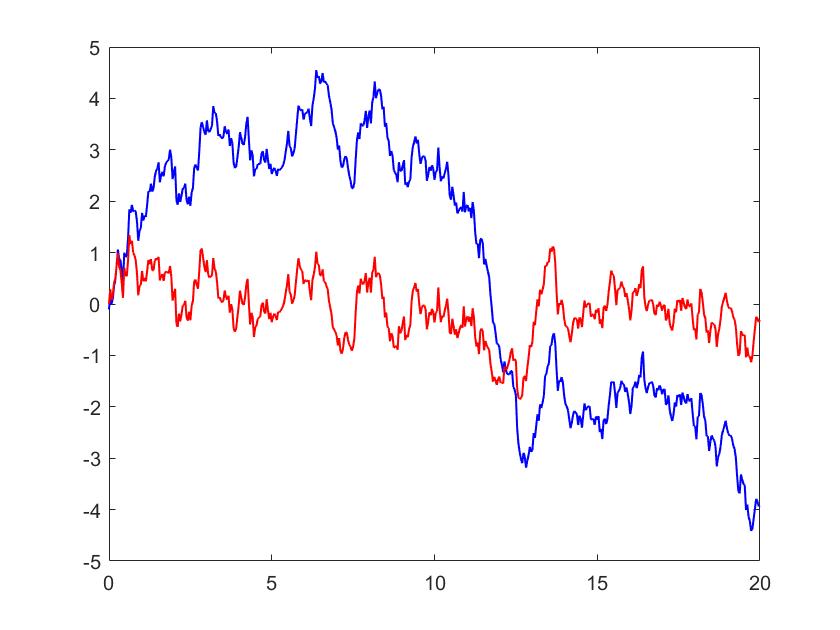
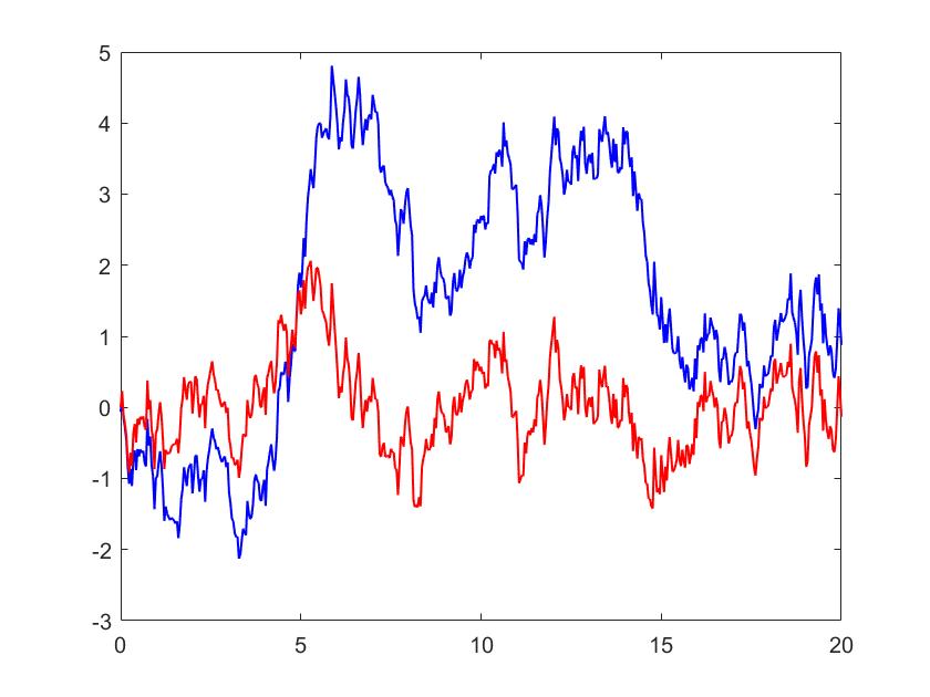
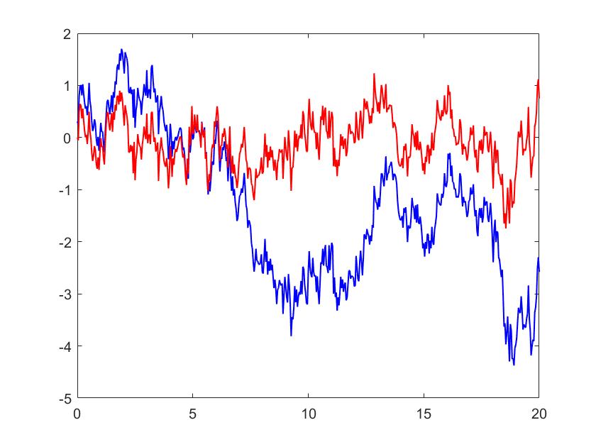
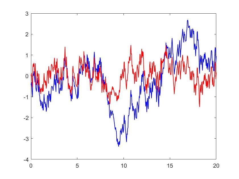
Figure 6.1: Sample Paths of fBM and fOU. From left to right and from top to bottom, $H=0.50,0.45,0.40,0.35$, respectively. Blue paths are fBM while red paths are fOU.

By our theory, the discretized rough path estimator $\widetilde{\gamma}_{n}$ in this model is given by

$$\widetilde{\gamma}_{n}(\omega)=-\frac{\sum_{\ell=1}^{n-1}X_{\ell h}(\omega)X_{\ell h,(\ell+1)h}(\omega)+\mathbb{X}_{\ell h,(\ell+1)h}(\omega)}{\sum_{\ell=1}^{n}X_{\ell h}(\omega)^{2}h},$$ (6.2)

where $X_{\ell h,(\ell+1)h}(\omega)=X_{(\ell+1)h}(\omega)-X_{\ell h}(\omega)$ are increments of sample path $X(\omega)$ and the second level/Lévy area

$$\begin{split}\mathbb{X}_{\ell h,(\ell+1)h}(\omega)&=\mathbb{X}_{\ell h,(\ell+1)h}^{\circ}(\omega)-\varphi_{\ell h,(\ell+1)h}\\ &=\int_{\ell h}^{(\ell+1)h}X_{\ell h,u}(\omega)\circ d_{\mathfrak{R}_{1}}\mathbf{X}(\omega)-\varphi_{\ell h,(\ell+1)h}\\ &=\frac{1}{2}(X_{(\ell+1)h}(\omega)-X_{\ell h}(\omega))^{2}-\varphi_{\ell h,(\ell+1)h},\end{split}$$

where $\varphi_{\ell h,(\ell+1)h}=\varphi((\ell+1)h)-\varphi(\ell h)$, $\varphi(t)=\frac{1}{2}t^{2H}-U(t)$, and

$$U(t)=2H\int_{0}^{t}\int_{0}^{s}e^{-2(s-u)}(s^{2H-1}-(s-u)^{2H-1})duds.$$

In summary, $(X_{\ell h,(\ell+1)h}(\omega),\mathbb{X}_{\ell h,(\ell+1)h}(\omega))_{\ell=0,1,\cdots,n-1}$ are our discrete observation for estimation. Note that since the dimension $d=1$ in this model, there is no Lévy area to be discretized. In the real world application such as the Vasicek interest rate model, the problem left for estimation is how to enhance high-frequency data to Itô rough path. We may refer to [6] as an inspiration for answering this problem.

We illustrate our simulation results in Table 1, where, one can see the mean and standard deviation of our discretized rough path estimators $\widetilde{\gamma}_{n}(\omega)$ for varying Hurst parameter $H$ based on 1000 Monte Carlo iterations of sample path $X(\omega)$. We take the time horizon $T=\{20,30,40\}$, sample size $n=\{2^{10},2^{11},2^{12}\}$, and Hurst parameter $H=\{0.50,0.45,0.40,0.35\}$. From Table 1, we can see that the estimated values are very good. The mean is very close to the true parameter value $\gamma=2$, and the standard deviation is small. That means the estimators are stable for each sample path.

Table 1: Mean and standard deviation of rough path estimators based on 1000 Monte Carlo iterations in dimension $d=1$, $n$ sample size, $T$ time horizon, $H$ Hurst parameter, and true parameter value $\gamma=2$.

		$H=0.50$		$H=0.45$		$H=0.40$		$H=0.35$
$T$	$n$	Mean	Std dev	Mean	Std dev	Mean	Std dev	Mean	Std dev
20	$2^{10}$	2.0636	0.4606	2.0349	0.4219	2.0284	0.3668	1.9946	0.3341
	$2^{11}$	2.0669	0.4517	2.0513	0.4173	2.0219	0.3645	2.0268	0.3353
	$2^{12}$	2.0734	0.4667	2.0667	0.4312	2.0361	0.3615	2.0270	0.3308
30	$2^{10}$	1.9972	0.3655	1.9963	0.3442	1.9573	0.2847	1.9646	0.2648
	$2^{11}$	2.0351	0.3694	2.0381	0.3316	2.0183	0.3092	2.0015	0.2648
	$2^{12}$	2.0557	0.3581	2.0358	0.3342	2.0206	0.3045	2.0249	0.2597
40	$2^{10}$	1.9687	0.3067	1.9418	0.2789	1.9365	0.2516	1.9239	0.2289
	$2^{11}$	2.0052	0.3075	1.9918	0.2892	1.9807	0.2625	1.9840	0.2206
	$2^{12}$	2.0284	0.3090	2.0100	0.2720	2.0056	0.2549	2.0003	0.2306

In addition, we can see even more information about our rough path estimators from Table 1. Actually, the sample size $n$, time horizon $T$ and sampling frequency $h=\frac{T}{n}$ affect the value of these estimators for different Hurst parameter $H$. One can see that when sample size $n$ fixed, as time horizon $T=nh$ becomes larger, the mean and standard deviation become smaller. When time horizon $T$ fixed, as sample size $n$ becomes large, the estimated values change regularly according to $T$. One may notice that it does not become better even if $T$ and $n$ become larger and larger. The reason behind that is $T$ and $n$ are not the only two variables which effect the estimator. Actually, the sampling frequency $h$ also works. The assumption in Theorem 5.1

$$T=nh\to\infty,\ h\to 0,\ nh^{p}\to 0,\ \mathrm{as}\ n\to\infty,$$ (6.3)

for some $p\in(1,\frac{1+H+\beta}{1+\beta})$, is very important when one computes the value of estimator. The three limits above mean that the convergence rate of mesh size/sampling frequency should be not too slow or too large. One should give a proper mesh size/sampling frequency $h$ in order to obtain better value of estimator. Besides, the proper sampling frequency $h$ also depends on Hurst parameter $H$. In Table 1, when $T,n,h$ are fixed, the mean value and standard deviation both become smaller. It is better to use different sampling frequency $h$ according to Hurst parameter $H$.

Following is a Box-and-Whisker Plot, in which the central red mark of each blue box indicates the median of rough path estimators $\widetilde{\gamma}_{n}(\omega)$ based on 1000 Monte Carlo iterations of sample paths $X(\omega)$, and the bottom and top edges of the box indicate the 25th and 75th percentiles, respectively. Besides, the outliers are plotted individually using the red ’+’ symbol.

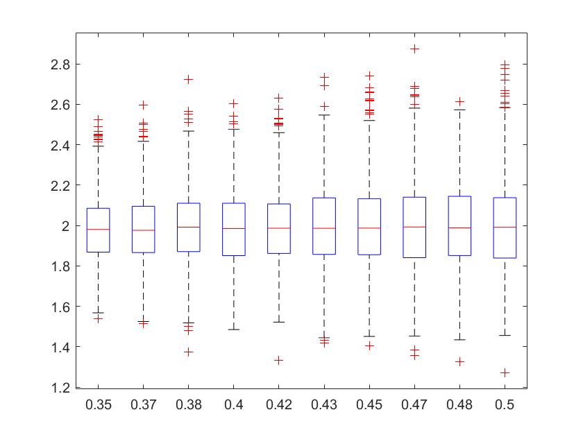
Figure 6.2: Box-Whisker plot of rough path estimator $\widetilde{\gamma}_{n}$ of 1000 Monte Carlo simulation, x-label is Hurst parameter $H$ from 0.35 to 0.50. Here, time horizon $T=80$, sample size $n=2^{13}$.

6.2 Two-dimensional example

In this subsection, we give numerical examples for two dimensional fOU processes, for example, the dynamics

$$dX_{t}=-\Gamma X_{t}dt+dB_{t}^{H},\ X_{0}=0,\ t\in[0,T],$$ (6.4)

with parameter matrix

$$\Gamma=\left(\begin{matrix}1&2\\ 2&5\end{matrix}\right).$$

That is,

$$dX_{t}^{1} =-(X_{t}^{1}+2X_{t}^{2})dt+dB_{t}^{H,1},$$

$$dX_{t}^{2} =-(2X_{t}^{1}+5X_{t}^{2})dt+dB_{t}^{H,2}.$$

We still apply Euler scheme to draw $n$ equidistant samples $\{X_{h}(\omega),X_{2h}(\omega),\cdots,X_{nh}(\omega)\}$ on time horizon $T$ with frequency $h=\frac{T}{n}$. In Figure 6.3, we show the paths of components of two dimensional fBM and its associated fOU process with $H=0.45$. $B^{H,1}$ and $B^{H,2}$ are independent, and $X^{1}$ and $X^{2}$ locally look like $B^{H,1}$ and $B^{H,2}$, respectively, for this model. In order to estimate the parameter matrix, we should enhance sample paths to data in rough path sense. That is, to get $\{(X_{\ell h,(\ell+1)h}(\omega),\mathbb{X}_{\ell h,(\ell+1)h}(\omega))_{\ell=0,1,\cdots,n-1}\}$ as our observation data for estimation.

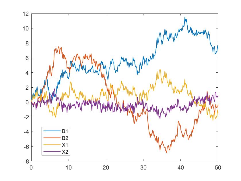
Figure 6.3: An example of sample paths of two-dimension fBM $(B1,B2)$ and fOU $(X1,X2)$ with $H=0.45$.

For dimension $d=2$, the continuous rough path estimator $\widehat{\Gamma}_{T}(\omega)=(\widehat{\Gamma}_{T}^{ij}(\omega))_{i,j=1,2}$ is given by

$$\begin{split}\widehat{\Gamma}_{T}^{ij}(\omega)&=-\frac{1}{V_{T}(X(\omega))}\left(\int_{0}^{T}(X_{s}^{3-j}(\omega))^{2}ds\int_{0}^{T}X_{s}^{j}(\omega)d_{\mathfrak{R}_{1}}\mathbf{X}^{i}(\omega)\right.\\ &\ \ \ \ \ \ \ \ \ \ \ \ \ \ \ \left.-\int_{0}^{T}X_{s}^{i}(\omega)X_{s}^{3-i}(\omega)ds\int_{0}^{T}X_{s}^{3-j}(\omega)d_{\mathfrak{R}_{1}}\mathbf{X}^{i}(\omega)\right),\end{split}$$ (6.5)

where

$$V_{T}(X(\omega))=\int_{0}^{T}(X_{s}^{1}(\omega))^{2}ds\int_{0}^{T}(X_{s}^{2}(\omega))^{2}ds-\left(\int_{0}^{T}X_{s}^{1}(\omega)X_{s}^{2}(\omega)ds\right)^{2},$$

and all the rough integrals above are defined in our Itô sense. Discretizing every integral above, we obtain our high frequency rough path estimator. The attention we need pay to is the cross term of rough integral, i.e. Lévy area $\int X^{i}d_{\mathfrak{R}_{1}}\mathbf{X}^{j}$ or $\mathbb{X}^{ij}$. Since

$$\mathbb{X}_{s,t}^{ij}=\mathbb{X}_{s,t}^{\circ,ij}-\varphi_{s,t},$$

where $\varphi_{s,t}$ is defined in section 2 and $\mathbb{X}_{s,t}^{\circ,ij}$ denotes the second level/Lévy area of fOU rough path enhancement in the Stratonovich sense. Now we can discretize the Stratonovich’s Lévy area $\mathbb{X}^{\circ,ij}$ by trapezoidal scheme, see [29]. By this, we get $\{(X_{\ell h,(\ell+1)h}(\omega),\mathbb{X}_{\ell h,(\ell+1)h}(\omega))_{\ell=0,1,\cdots,n-1}\}$ as our discrete observation data for estimation.

We illustrate our two dimensional simulation results in Table 2 below. In this case, we estimate the parameter matrix $\Gamma$ using the simulated data $\{(X_{\ell h,(\ell+1)h}(\omega),\mathbb{X}_{\ell h,(\ell+1)h}(\omega))_{\ell=0,1,\cdots,n-1}\}$. We draw 1000 sample paths by Monte Carlo iterations.

Table 2: Mean and standard deviation of rough path estimators $\widetilde{\Gamma}_{n}$ based on 1000 Monte Carlo iterations in dimension $d=2$, $n$ sample size, $T$ time horizon, $h$ sampling frequency, $H$ Hurst parameter, and true parameter matrix $\Gamma=[1\ 2;\ 2\ 5]$.

	$n=2^{11}$	$n=2^{12}$	$n=2^{13}$
$H=0.50$	$T=20,h=0.0098$	$T=30,h=0.0073$	$T=40,h=0.0049$
Mean	$\left(\begin{matrix}1.0956&1.9720\\ 1.9765&5.0381\end{matrix}\right)$	$\left(\begin{matrix}1.0548&1.9579\\ 1.9918&5.0443\end{matrix}\right)$	$\left(\begin{matrix}1.0551&2.0091\\ 1.9848&5.0146\end{matrix}\right)$
Std dev	$\left(\begin{matrix}0.3350&0.6824\\ 0.3374&0.7399\end{matrix}\right)$	$\left(\begin{matrix}0.2755&0.5955\\ 0.2719&0.5590\end{matrix}\right)$	$\left(\begin{matrix}0.2429&0.5142\\ 0.2313&0.4984\end{matrix}\right)$
$H=0.45$	$T=13,h=0.0063$	$T=22,h=0.0054$	$T=40,h=0.0049$
Mean	$\left(\begin{matrix}1.1163&1.9832\\ 1.9889&5.1160\end{matrix}\right)$	$\left(\begin{matrix}1.0731&1.9943\\ 1.9665&5.0106\end{matrix}\right)$	$\left(\begin{matrix}1.0449&2.0105\\ 1.9744&4.9902\end{matrix}\right)$
Std dev	$\left(\begin{matrix}0.4135&0.9030\\ 0.4429&0.8453\end{matrix}\right)$	$\left(\begin{matrix}0.3172&0.6914\\ 0.3034&0.6128\end{matrix}\right)$	$\left(\begin{matrix}0.2169&0.4743\\ 0.2166&0.4517\end{matrix}\right)$
$H=0.40$	$T=14,h=0.0068$	$T=20,h=0.0049$	$T=35,h=0.0043$
Mean	$\left(\begin{matrix}1.1030&2.0077\\ 1.9767&5.0416\end{matrix}\right)$	$\left(\begin{matrix}1.0585&1.9836\\ 1.9895&5.0283\end{matrix}\right)$	$\left(\begin{matrix}1.0361&1.9946\\ 1.9790&4.9894\end{matrix}\right)$
Std dev	$\left(\begin{matrix}0.3745&0.8473\\ 0.3878&0.7160\end{matrix}\right)$	$\left(\begin{matrix}0.3200&0.7466\\ 0.3242&0.6152\end{matrix}\right)$	$\left(\begin{matrix}0.2275&0.5441\\ 0.2367&0.4517\end{matrix}\right)$
$H=0.35$	$T=14,h=0.0068$	$T=20,h=0.0049$	$T=30,h=0.0037$
Mean	$\left(\begin{matrix}1.0724&1.9606\\ 1.9588&4.9324\end{matrix}\right)$	$\left(\begin{matrix}1.0555&2.0065\\ 1.9645&4.9839\end{matrix}\right)$	$\left(\begin{matrix}1.0298&1.9927\\ 1.9796&4.9908\end{matrix}\right)$
Std dev	$\left(\begin{matrix}0.3612&0.8816\\ 0.3796&0.6448\end{matrix}\right)$	$\left(\begin{matrix}0.3074&0.7608\\ 0.3234&0.5628\end{matrix}\right)$	$\left(\begin{matrix}0.2448&0.6067\\ 0.2488&0.4453\end{matrix}\right)$

In Table 2, every component of ’Mean’ denotes average of the value of respective estimator based on 1000 Monte Carlo simulation. And the component of ’Standard deviation (Std dev)’ represents the fluctuation of estimation of parameter with corresponding index. One could see that, under proper time horizon $T$, sample size $n$ and frequency $h$, the rough path estimator performs very well and the results are quite stable.

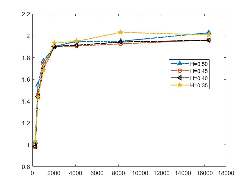
Figure 6.4: Curves of mean of $\widetilde{\Gamma}_{n}^{12}$ based on 100 Monte Carlo simulated paths, time horizon $T=40$ fixed, x-label $n$ from $2^{8}$ to $2^{14}$.

As a remark, in one dimensional case, we have seen that the performance of discrete estimator dependents on time horizon $T$, sample size $n$ and frequency $h$. But it is not so sensitive in dimension $d=1$ so that we can still use the same sample setting for varying Hurst parameter $H$. However, in dimension $d=2$, it becomes a little sensitive to sampling mode. One should adhere to the conditions about $T,n,h$ in Theorem 5.1 in order to obtain better estimated values. In Table 2, we set frequency $h$ becomes smaller as sample size $n$ becomes larger and Hurst parameter $H$ smaller.

In Figure 6.4, we fix time horizon $T=40$, and take sample sizes $n=2^{8},2^{9},\cdots,2^{14}$. We show the trend of mean of estimated values $\widetilde{\Gamma}_{n}^{12}$ (as an example) with respect to sample size $n$ based on 100 Monte Carlo simulated sample paths. As one can see, when sample size $n$ is too small or observation frequency $h=\frac{T}{n}$ too large, the estimated values are bad. However, as expected, the estimation becomes good with $n$ increasing or $h$ decreasing, and stabilised at the exact value $\Gamma^{12}=2$.

References

- [1] Y. Aït Sahalia. Maximum likelihood estimation of discretely sampled diffusions: a closed form approximation approach. Econometrica, 70, 223-262 (2002).
- [2] Y. Aït-Sahalia, J. Jacod. Estimating the degree of activity of jumps in high frequency financial data. Annals of Statistics, 37, 2202-2244 (2009).
- [3] Y. Aït-Sahalia, J. Jacod. Is Brownian motion necessary to model high frequency data? Annals of Statistics, 38, 3093-3128 (2010).
- [4] Y. Aït-Sahalia, J. Jacod. High-Frequency Financial Econometrics. Princeton University Press, (2014).
- [5] Y. Aït-Sahalia, P. Mykland, L. Zhang. Ultra high frequency volatility estimation with dependent microstructure noise. Journal of Econometrics, 160, 160-175 (2011).
- [6] I. Bailleul, J. Diehl. The Inverse Problem for Rough Controlled Differential Equations. SIAM J. Control Optim., 53, 5, 2762-2780 (2015).
- [7] A. Beskos, O. Papaspiliopoulos, G. Roberts. Monte Carlo maximum likelihood estimation for discretely observed diffusion processes. Annals of Statistics, 37, 223-245 (2009).
- [8] R. Carmona, J. Fouque, L. Sun. Mean field games and systemic risk. Commun. Math. Sci., 13, 4, 911-933 (2015).
- [9] P. Cheridito, H. Kawaguchi, M. Maejima, Fractional Ornstein-Uhlenbeck processes. Electron. J. Probab. 8, 1-14 (2003).
- [10] F. Comte, V. Genon-Catalot. Estimation for Lévy processes from high frequency data within a long time interval. Annals of Statistics, 39, 803-837 (2011).
- [11] L. Coutin, Z. Qian. Stochastic analysis, rough path analysis and fractional Brownian motions. Probab. Theory Relat. Fields, 122, 108-140 (2002).
- [12] J. Diehl, P. Friz, H. Mai. Pathwise stability of likelihood estimators for diffusions via rough paths, Ann. Appl. Probab., 26, 4, 2169-2192 (2016).
- [13] V. Fasen. Statistical estimation of multivariate Ornstein-Uhlenbeck processes and applications to co-integration, J. Econometrics, 172, 2, 325-337 (2013).
- [14] J. Fouque, T. Ichiba. Stability in a model of interbank lending. SIAM J. Financial Math., 4, 1, 784-803 (2013).
- [15] P. Friz, M. Hairer. A Course on Rough Paths: With an Introduction to Regularity Structures, Springer, New York (2014).
- [16] P. Friz, N. Victoir. Multidimensional Stochastic Processes as Rough Paths. Theory and Applications. Cambridge Studies in Advanced Mathematics, 120. Cambridge Univ. Press, Cambridge, 2010.
- [17] M. Gubinelli. Controlling rough paths. J. Functional Analysis, 216, 1, 86-140 (2004).
- [18] Y. Hu. Analysis on Gaussian spaces. World Scientific Publishing Co. Pte. Ltd., Hackensack, NJ (2017). ISBN 978-981-3142-17-6.
- [19] Y. Hu, D. Nualart. Parameter estimation for fractional Ornstein-Uhlenbeck processes. Stat. Probab. Lett., 80, 11-12, 1030-1038 (2010).
- [20] Y. Hu, D. Nualart, H. Zhou. Parameter estimation for fractional Ornstein-Uhlenbeck processes of general Hurst parameter, Stat. Inference Stoch. Process. (2017).
- [21] J. Jacod, A.N. Shiryaev. Limit Theorems for Stochastic Processes, 2nd ed. Springer-Verlag, (2003).
- [22] M.L. Kleptsyna, A. Le Breton. Statistical analysis of the fractional Ornstein-Uhlenbeck type process. Stat. Inference Stoch. Process. 5, 229-248 (2002).
- [23] R.S. Liptser, A.N. Shiryaev. Statistics of Random Processes, I. General Theory. Springer-Verlag New York, (1977).
- [24] R.S. Liptser, A.N. Shiryaev. Statistics of Random Processes, II. Applications. Springer-Verlag New York, (1978).
- [25] T. Lyons. Differential equations driven by rough signals. Rev. Mat. Iberoamericana, 14, 215-310 (1998).
- [26] T. Lyons, M. Caruana, and T. Lévy. Differential equations driven by rough paths. Springer, 2007.
- [27] T. Lyons, Z. Qian. System Control and Rough Paths. Oxford Univ. Press, Oxford (2002). M
- [28] P. Mykland, L. Zhang. Inference for continuous semimartingales observed at high frequency. Econometrica, 77,1403-1445 (2009).
- [29] A. Neuenkirch, S. Tindel, J. Unterberger. Discretizing the fractional Lévy area, Stoc. Process Appl., 120, 223-254 (2010).
- [30] R. Norvaisa, Weighted power variation of integrals with respect to a Gaussian process. Bernoulli, 21, 2, 1260-1288 (2015).
- [31] A. Papavasiliou, C. Ladroue. Parameter estimation for rough differential equations. Annals of Statistics, 39, 4, 2047-2073 (2011).
- [32] J. Pickands, Asymptotic properties of the maximum in a stationary Gaussian process. Trans. Am. Math. Soc., 145, 75-86 (1969).
- [33] V. Pipiras, M.S. Taqqu. Integration questions related to fractional Brownian motion, Probab. Theory Related Fields, 118, 251-291 (2000).
- [34] Z. Qian, X. Xu. Itô integrals for fractional Brownian motion and application to option pricing, ArXiv Mathematics e-prints (2018). arXiv: 1803.00335v1.
- [35] P. Rao, Semimartingales and their Statistical Inference, Chapman & Hall/CRC, (1999).
- [36] P. Rao, Statistical Inference for Diffusion Type Processes, Arnold, (1999).
- [37] D.W. Stroock, S.R.S. Varadhan, Multidimensional Diffusion Processes. Springer-Verlag, Berlin, Germany (1979).
- [38] C. Tudor, F. Viens. Statistical aspects of the fractional stochastic calculus. Annals of Statistics, 35, 3, 1183-1212 (2007).