Symmetric and Asymmetric Wormholes Immersed In Rotating Matter

Abstract

We consider four-dimensional wormholes immersed in bosonic matter. While their existence is based on the presence of a phantom field, many of their interesting physical properties are bestowed upon them by an ordinary complex scalar field, which carries only a mass term, but no self-interactions. For instance, the rotation of the scalar field induces a rotation of the throat as well. Moreover, the bosonic matter need not be symmetrically distributed in both asymptotically flat regions, leading to symmetric and asymmetric rotating wormhole spacetimes. The presence of the rotating matter also allows for wormholes with a double throat.

I Introduction

In General Relativity the non-trivial topology of wormholes can be achieved by allowing for the presence of exotic matter Ellis:1973yv ; Bronnikov:1973fh ; Kodama:1978dw ; Ellis:1979bh ; Morris:1988cz ; Morris:1988tu ; Lobo:2005us ; Lobo:2017oab . In the simplest case, a massless phantom (scalar) field can be chosen, whose Lagrangian carries the opposite sign as compared to the one of an ordinary scalar field. The resulting Ellis wormholes are static spherically symmetric solutions, connecting two asymptotically flat regions of space-time.

Ellis wormholes may also be coupled to matter fields. For instance, they may be filled by nuclear matter Dzhunushaliev:2011xx ; Dzhunushaliev:2012ke ; Dzhunushaliev:2013lna ; Dzhunushaliev:2014mza ; Aringazin:2014rva ; Dzhunushaliev:2016ylj , they may be threaded by chiral (Skyrmionic) matter Charalampidis:2013ixa , or they may be immersed in bosonic matter consisting of an ordinary complex boson field with self-interaction Dzhunushaliev:2014bya ; Hoffmann:2017jfs , or with only a mass term present Hoffmann:2017vkf .

As in the case of non-topological solitons and boson stars Jetzer:1991jr ; Lee:1991ax ; Schunck:2003kk ; Liebling:2012fv the boson field then has a harmonic time-dependence, allowing for localized matter fields surrounding a static throat. Since the time-dependence cancels in the stress-energy tensor, the resulting metric is static. Clearly, there are symmetric wormholes, where the matter is distributed symmetrically on either side of the throat. Thus these symmetric wormholes possess reflection symmetry. Due to the non-trivial topology, however, also wormhole solutions appear, where the matter is distributed unevenly with respect to the spacetime regions on either side of the throat. These asymmetric wormholes always appear in pairs, where the two solutions of a pair are again related via reflection symmetry.

Ellis wormholes may also rotate Kashargin:2007mm ; Kashargin:2008pk ; Kleihaus:2014dla ; Chew:2016epf ; Kleihaus:2017kai . A rotation of the throat can be induced by an appropriate choice of the boundary conditions, allowing for asymptotic flatness in the two asymptotic regions, which, however, are rotating with respect to one another. On the other hand, a rotation of the throat can also be induced by immersing the throat into rotating matter Hoffmann:2017vkf . In that case, the boundary conditions can be chosen symmetrically in the two asymptotic regions, and thus these need not rotate with respect to one another.

These wormholes immersed in rotating matter possess interesting properties Hoffmann:2017vkf . Depending on their physical parameters, their geometry can change from exhibiting a single throat to developing an equator surrounded by a throat on either side, i.e., these wormholes then feature a double throat geometry. These wormholes also possess ergoregions and an interesting lightring structure. Here we show that, like their non-rotating counterparts, they also come in two versions, namely symmetric and asymmetric wormholes, where the asymmetric wormholes again always come in pairs related to each other via reflection symmetry.

The study of rotating wormholes is rather attractive from an astrophysical point of view, since rotation is ubiquitous in the Universe, and first astrophysical searches for wormholes have already been carried out Abe:2010ap ; Toki:2011zu ; Takahashi:2013jqa . In this respect studies of the properties of wormholes as gravitational lenses are highly relevant Cramer:1994qj ; Safonova:2001vz ; Perlick:2003vg ; Nandi:2006ds ; Nakajima:2012pu ; Tsukamoto:2012xs ; Kuhfittig:2013hva ; Tsukamoto:2016zdu , and so are studies of their shadows Bambi:2013nla ; Nedkova:2013msa together with the signatures of accretion disks surrounding them Zhou:2016koy ; Lamy:2018zvj .

Here we investigate the basic physical properties of wormholes immersed in rotating bosonic matter, which does not possess any self-interaction, focusing on the new aspect of the presence of symmetric and asymmetric solutions. The set of field equations is symmetric with respect to reflection of the radial coordinate at the center, and the boson field and the metric possess the same boundary conditions in both asymptotically flat regions. The solutions, however, may be either symmetric or asymmetric with respect to such a reflection, and asymmetric solutions exist at least within a certain domain of the parameter space.

We remark that the solutions investigated here are quite different from those (non-rotating) solutions studied before, which are based on a complex boson field with a sextic self-interaction Hoffmann:2017jfs . There, the mechanism of spontaneous symmetry breaking arises, which is known in diverse contexts in physics, ranging from ferromagnetic materials to the generation of mass of the elementary particles via the Higgs mechanism (see e.g., Strocchi:2008gsa ). It applies to systems, where the ground state of a system does not display the full symmetry of the underlying set of equations.

The paper is organized as follows. In section II we provide the theoretical setting for the wormhole solutions. We present the action, the Ansätze, the equations of motion, the boundary conditions, as well as the expressions for the global charges, the geometrical properties, and the lightrings. In section III we first demonstrate that for the present case of a boson field with a mass term only, there are no non-trivial solutions in the probe limit. Subsequently we address the solutions of the fully gravitating system, starting with the non-rotating case. For the rotating case we then consider solutions with the lowest values of the rotational quantum number, entering the Ansatz for the boson field analogously to the well-known case of rotating boson stars Schunck:1996 ; Schunck:1996he ; Ryan:1996nk ; Yoshida:1997qf ; Schunck:1999pm ; Kleihaus:2005me ; Kleihaus:2007vk . In particular, we analyze their global charges, discuss their bifurcations, illustrate their geometrical properties, and address their lightring structure. We end with our conclusions in section IV.

II Theoretical setting

In the following we first present the action employed for obtaining wormholes in the presence of rotating bosonic matter. We then discuss the Ansätze for the metric and the scalar fields, exhibit the resulting set of field equations, and present an adequate set of symmetric boundary conditions. Subsequently we discuss the global charges of the solutions. We present the formulae for the analysis of their geometrical properties, including their throat(s) and equator, and we provide the basis for the analysis of their lightrings.

II.1 Action

We start from an action in four spacetime dimensions, where General Relativity is minimally coupled to a complex scalar field $\Phi$ and a real phantom field $\Psi$. The action $S$

$$S=\int\left[\frac{1}{2\kappa}{\cal R}+{\cal L}_{\rm ph}+{\cal L}_{\rm bs}\right]\sqrt{-g}\ d^{4}x$$ (1)

then contains besides the Einstein-Hilbert action with curvature scalar $\cal R$, coupling constant $\kappa=8\pi G$ and metric determinant $g$, the respective matter contributions, the Lagrangian ${\cal L}_{\rm bs}$ of the complex scalar field $\Phi$

$${\cal L}_{\rm bs}=-\frac{1}{2}g^{\mu\nu}\left(\partial_{\mu}\Phi^{*}\partial_{\nu}\Phi+\partial_{\nu}\Phi^{*}\partial_{\mu}\Phi\right)-m_{\rm bs}^{2}|\Phi|^{2}\ ,$$ (2)

where the asterisk denotes complex conjugation and $m_{\rm bs}$ denotes the boson mass, as well as the Lagrangian ${\cal L}_{\rm ph}$ of the phantom field $\Psi$,

$${\cal L}_{\rm ph}=\frac{1}{2}\partial_{\mu}\Psi\partial^{\mu}\Psi\ ,$$ (3)

which carries the reverse sign as compared to the kinetic term of the complex scalar field $\Phi$ Ellis:1973yv ; Bronnikov:1973fh ; Kodama:1978dw ; Ellis:1979bh ; Morris:1988cz ; Morris:1988tu ; Lobo:2005us ; Lobo:2017oab .

By varying the action with respect to the metric we obtain the Einstein equations

$$G_{\mu\nu}={\cal R}_{\mu\nu}-\frac{1}{2}g_{\mu\nu}{\cal R}=\kappa T_{\mu\nu}$$ (4)

with stress-energy tensor

$$T_{\mu\nu}=g_{\mu\nu}{{\cal L}}_{M}-2\frac{\partial{{\cal L}}_{M}}{\partial g^{\mu\nu}}\ ,$$ (5)

where we have denoted the sum of the scalar field Lagrangians by ${\cal L}_{M}={\cal L}_{\rm ph}+{\cal L}_{\rm bs}$. By varying with respect to the scalar fields we obtain the phantom field equation

$$\nabla^{\mu}\nabla_{\mu}\Psi=0\ ,$$ (6)

and the equation for the complex scalar field

$$\nabla^{\mu}\nabla_{\mu}\Phi=m_{\rm bs}^{2}\Phi\ .$$ (7)

For convenience we introduce dimensionless scalar fields and a dimensionless coordinate

$$\hat{\Phi}=\sqrt{\kappa}\Phi\ ,\ \ \ \hat{\Psi}=\sqrt{\kappa}\Psi\ ,\ \ \ \hat{\eta}=\frac{1}{\lambda}\eta\ ,$$ (8)

yielding

$$\hat{G}_{\mu\nu}=\hat{T}_{\mu\nu}\ ,$$ (9)

where the mass term of the complex boson field $\hat{m}_{\rm bs}^{2}|\hat{\Phi}|^{2}$ now contains the dimensionless mass parameter

$$\hat{m}_{\rm bs}=\left(\frac{m_{\rm bs}}{m_{\rm P}}\right)\left(\frac{M_{0}}{m_{\rm P}}\right)\ ,$$ (10)

with the mass scale $M_{0}$ being related to the length scale by $M_{0}=\lambda/G$, and $m_{\rm P}$ denotes the Planck mass. Throughout the paper we will choose $\hat{m}_{\rm bs}=\sqrt{1.1}$. In the following we will omit the hats again for simplicity.

II.2 Ansätze

The line element for the metric incorporates the non-trivial topology of the wormhole solutions,

$$ds^{2}=-e^{f}dt^{2}+e^{q-f}\left[e^{b}(d\eta^{2}+hd\theta^{2})+h\sin^{2}\theta(d\varphi-\omega dt)^{2}\right]\ ,$$ (11)

where $f$, $q$, $b$ and $\omega$ are functions of the radial coordinate $\eta$ and the polar angle $\theta$, and $h=\eta^{2}+\eta_{0}^{2}$ is an auxiliary function, which contains the throat parameter $\eta_{0}$. The radial coordinate $\eta$ takes positive and negative values, i.e. $-\infty<\eta<\infty$. The two limits $\eta\to\pm\infty$ correspond to two distinct asymptotically flat regions, associated with ${\cal M}_{+}$ and ${\cal M}_{-}$, respectively.

For the complex scalar field $\Phi$ we adopt the same Ansatz as the one usually employed for rotating $Q$-balls and boson stars Schunck:1996 ; Schunck:1996he ; Ryan:1996nk ; Yoshida:1997qf ; Schunck:1999pm ; Kleihaus:2005me ; Kleihaus:2007vk ,

$$\Phi(t,\eta,\theta,\varphi)=\phi(\eta,\theta)\leavevmode\nobreak\ e^{i\omega_{s}t+in\varphi}\ ,$$ (12)

where $\phi(\eta,\theta)$ is a real function, $\omega_{s}$ denotes the real boson frequency, and $n$ is the integer winding number or rotational quantum number. Finally, the Ansatz for the phantom field $\Psi$ is chosen to depend only on the coordinates $\eta$ and $\theta$,

$$\Psi(t,\eta,\theta,\varphi)=\psi(\eta,\theta)\ .$$ (13)

II.3 Einstein and Matter Field Equations

After substituting the above Ansätze into the Einstein equations $E_{\mu}^{\nu}=G_{\mu}^{\nu}-T_{\mu}^{\nu}=0$ we obtain the following set of coupled field equations

$$f_{,\eta\eta}+\frac{f_{,\theta\theta}}{h}+f_{,\eta}\frac{hq_{,\eta}+4\eta}{2h}+f_{,\theta}\frac{2\cot\theta+q_{,\theta}}{2h}-e^{q-2f}\sin^{2}\theta\left(h\omega_{,\eta}^{2}+\omega_{,\theta}^{2}\right)=4\left[2(n\omega+\omega_{s})^{2}-m_{\rm bs}^{2}e^{f}\right]e^{b+q-2f}\phi^{2}\ ,$$ (14)

$$q_{,\eta\eta}+\frac{q_{,\theta\theta}}{h}+\frac{q_{,\eta}^{2}}{2}+\frac{3\eta q_{,\eta}}{h}+\frac{q_{,\theta}^{2}}{2h}+\frac{2q_{,\theta}\cot\theta}{h}=8\left(e^{q-2f}h\left[(n\omega+\omega_{s})^{2}-m_{\rm bs}^{2}e^{f}\right]\sin^{2}\theta-n^{2}\right)\phi^{2}\frac{e^{b}}{h\sin^{2}\theta}\ ,$$ (15)

$$b_{,\eta\eta}+\frac{b_{,\theta\theta}}{h}+b_{,\eta}\frac{\eta}{h}$$ (16)

$$+\frac{1}{2}\left(f_{,\eta}^{2}+\frac{f_{,\theta}^{2}}{h}-q_{,\eta}^{2}-\frac{q_{,\theta}^{2}}{h}-\frac{4}{h}\left(\cot\theta q_{,\theta}+\eta q_{,\eta}\right)+\frac{4}{h}\left(1-\frac{\eta^{2}}{h}\right)-3e^{q-2f}h\left(\omega_{,\eta}^{2}+\frac{\omega_{,\theta}^{2}}{h}\right)\sin^{2}\theta\right)$$

$$= 2\left(\psi_{,\eta}^{2}+\frac{\psi_{,\theta}^{2}}{h}\right)-4\left(\phi_{,\eta}^{2}+\frac{\phi_{,\theta}^{2}}{h}\right)-4\left(e^{q-2f}h\left[(n\omega+\omega_{s})^{2}-m_{\rm bs}^{2}e^{f}\right]\sin^{2}\theta-3n^{2}\right)\phi^{2}\frac{e^{b}}{h\sin^{2}\theta}\ ,$$

$$\omega_{,\eta\eta}+\frac{\omega_{,\theta\theta}}{h}+\frac{\omega_{,\eta}}{2}\left(3q_{,\eta}-4f_{,\eta}+\frac{8\eta}{h}\right)+\frac{\omega_{,\theta}}{2h}\left(3q_{,\theta}-4f_{,\theta}+6\cot\theta\right)=8n(n\omega+\omega_{s})\phi^{2}\frac{e^{b}}{h\sin^{2}\theta}\ ,$$ (17)

which result from $E^{t}_{t}=0$, $E^{\eta}_{\eta}+E^{\theta}_{\theta}=0$, $E^{\varphi}_{\varphi}=0$ and $E^{t}_{\varphi}=0$. The matter field equations are obtained from the Euler-Lagrange equations,

$$\partial_{\mu}\left(\frac{\partial L_{\rm m}}{\partial\phi_{,\mu}}\right)-\frac{\partial L_{\rm m}}{\partial\phi}=0\ ,\ \ \ \partial_{\mu}\left(\frac{\partial L_{\rm m}}{\partial\psi_{,\mu}}\right)-\frac{\partial L_{\rm m}}{\partial\psi}=0\ ,$$ (18)

where $L_{\rm m}=\left({\cal L}_{\rm bs}+{\cal L}_{\rm ph}\right)\sqrt{-g}$. They read

$$\phi_{,\eta\eta}+\frac{\phi_{,\theta\theta}}{h}+\frac{\phi_{,\eta}}{2}\left(q_{,\eta}+4\frac{\eta}{h}\right)+\frac{\phi_{,\theta}}{2h}\left(q_{,\theta}+2\cot\theta\right)+\left(e^{q-2f}h\left[(n\omega+\omega_{s})^{2}-m_{\rm bs}^{2}e^{f}\right]\sin^{2}\theta-n^{2}\right)\phi\frac{e^{b}}{h\sin^{2}\theta}=0\ ,$$ (19)

$$\psi_{,\eta\eta}+\frac{\psi_{,\theta\theta}}{h}+\frac{\psi_{,\eta}}{2}\left(q_{,\eta}+4\frac{\eta}{h}\right)+\frac{\psi_{,\theta}}{2h}\left(q_{,\theta}+2\cot\theta\right)=0\ .$$ (20)

This system of equations is symmetric with respect to reflection, $\eta\to-\eta$. Thus it allows for reflection symmetric solutions, i.e., solutions whose functions are either symmetric or antisymmetric under reflection symmetry, $\eta\to-\eta$. However, as we will see below, it also allows for solutions, which are asymmetric, when $\eta\to-\eta$. These asymmetric solutions, however, then always come in pairs, where the two solutions of a pair are related via the transformation $\eta\to-\eta$.

II.4 Boundary Conditions

In order to solve the above set of six coupled partial differential equations (PDEs) of second order, we have to impose boundary conditions for each function at the boundaries of the domain of integration consisting of the two asymptotic regions $\eta\to\pm\infty$, the axis of rotation $\theta=0$, and the equatorial plane $\theta=\pi/2$.

Our choice of boundary conditions is guided by considerations of symmetry. In particular, we here would like to impose symmetric boundary conditions for the metric and the complex boson field, i.e., boundary conditions which are the same for $\eta\to\infty$ and $\eta\to-\infty$. Then also symmetric solutions will be found, as briefly discussed in Hoffmann:2017jfs . However, asymmetric solutions arise as well, and in that case the asymmetry appearing in the solutions is not enforced via the boundary conditions.

Let us now detail our choice of boundary conditions. We demand in both asymptotic regions a Minkowski metric and a vanishing boson field

$$\left.f(\eta,\theta)\right|_{\eta\to\pm\infty}=\left.q(\eta,\theta)\right|_{\eta\to\pm\infty}=\left.b(\eta,\theta)\right|_{\eta\to\pm\infty}=\left.\omega(\eta,\theta)\right|_{\eta\to\pm\infty}=\left.\phi(\eta,\theta)\right|_{\eta\to\pm\infty}=0\ .$$ (21)

Along the rotation axis regularity requires

$$\left.\partial_{\theta}f(\eta,\theta)\right|_{\theta=0}=\left.\partial_{\theta}q(\eta,\theta)\right|_{\theta=0}=\left.\partial_{\theta}\omega(\eta,\theta)\right|_{\theta=0}=0\ ,\ \ \ \left.b(\eta,\theta)\right|_{\theta=0}=\left.\phi(\eta,\theta)\right|_{\theta=0}=0\ .$$ (22)

Imposing reflection symmetry with respect to the equatorial plane yields

$$\left.\partial_{\theta}f(\eta,\theta)\right|_{\theta=\frac{\pi}{2}}=\left.\partial_{\theta}q(\eta,\theta)\right|_{\theta=\frac{\pi}{2}}=\left.\partial_{\theta}b(\eta,\theta)\right|_{\theta=\frac{\pi}{2}}=\left.\partial_{\theta}\omega(\eta,\theta)\right|_{\theta=\frac{\pi}{2}}=\left.\partial_{\theta}\phi(\eta,\theta)\right|_{\theta=\frac{\pi}{2}}=0\ .$$ (23)

For the phantom field the boundary conditions need special care. Analogous to the other functions, regularity and reflection symmetry with respect to the equatorial plane require

$$\left.\partial_{\theta}\psi(\eta,\theta)\right|_{\theta=0}=\left.\partial_{\theta}\psi(\eta,\theta)\right|_{\theta=\frac{\pi}{2}}=0\ .$$ (24)

However, since only derivatives of the phantom field enter the PDEs, we can make any choice $\psi(\eta,\theta)\to\psi_{0}$ as $\eta\to\infty$. The boundary condition at $\eta=-\infty$ is then determined from the asymptotic form of the solutions as $\eta\to-\infty$,

$$\left\{2\eta^{2}\partial_{\eta}\left(\eta^{2}\partial_{\eta}b\right)+\sin^{2}\theta\left[\left(\eta^{2}\partial_{\eta}f\right)^{2}-4\left(\eta^{2}\partial_{\eta}\psi\right)^{2}+4\eta^{2}\partial_{\eta}\left(\eta^{2}\partial_{\eta}q\right)+4\eta_{0}^{2}\right]\right\}_{\eta\to-\infty}=0\ .$$ (25)

II.5 Mass, angular momentum and particle number

With each of the two distinct asymptotically flat regions, ${\cal M}_{\pm}$, we can associate a mass, $M_{\pm}$, an angular momentum, $J_{\pm}$, and a particle number, $Q_{\pm}$, where the signs of the global charges refer to the signs of ${\cal M}_{\pm}$. The mass and the angular momentum can be obtained from the asymptotic behaviour of the metric functions

$$f\longrightarrow\mp\frac{2M_{\pm}}{\eta}\ ,\ \ \ \omega\longrightarrow\frac{2J_{\pm}}{\eta^{3}}\ \ \ \ {\rm as}\ \eta\to\pm\infty\ .$$ (26)

For symmetric solutions the global charges are the same in both asymptotically flat regions. Therefore, we will omit the index $\pm$ for symmetric solutions. Their particle number $Q$ is related to the angular momentum $J$ via the well-known relation $J=nQ$ Schunck:1996 ; Schunck:1996he ; Ryan:1996nk ; Yoshida:1997qf ; Schunck:1999pm ; Kleihaus:2005me ; Kleihaus:2007vk which also holds in this case Hoffmann:2017vkf .

For the asymmetric solutions the values of the mass in the two asymptotic regions differ from each other, and so do the values of the angular momentum. However, because the two asymmetric solutions of a pair are related via $\eta\to-\eta$, their masses are related via $M_{\pm}\to M_{\mp}$, and likewise their angular momenta via $J_{\pm}\to J_{\mp}$.

For the asymmetric solutions also the extraction of the respective particle numbers $Q_{\pm}$ is more involved, since the choice of the inner boundary is ambiguous, when the usual integral over the time-component of the conserved current is performed, as discussed in Hoffmann:2017jfs . Therefore a trick may be applied, introducing a coupling to a fictitious electromagnetic field, such that the particle number can be read off asymptotically as the electric charge associated with the gauge field. This approach is outlined in Appendix A.

II.6 Geometrical properties

From the geometrical side it is most interesting to analyze the throat structure for these wormholes. To that end we consider the circumferential radius $R_{e}(\eta)$ in the equatorial plane,

$$R_{e}(\eta)=\sqrt{h}\left.e^{\frac{q-f}{2}}\right|_{\theta=\pi/2}\ .$$ (27)

The minima of the circumferential radius $R_{e}$ then correspond to throats, while the local maxima correspond to equators. Since the circumferential radius $R_{e}(\eta)$ increases without bound in the asymptotic regions, ${\cal M}_{\pm}$, any equator must reside between two throats.

For symmetric solutions the center $\eta=0$ will always correspond to either a throat or an equator. For asymmetric solutions this will no longer be the case. Here the location of the single throat will shift away from $\eta=0$, and when an equator arises, this can happen far from $\eta=0$, as well, as we will see below.

II.7 Ergoregion and lightrings

Further physical quantities of interest are the location of the ergoregion and the presence of lightrings. The condition $g_{tt}>0$ defines the ergoregion, i.e., it represents the region where the time-time component of the metric is positive. Its boundary is referred to as ergosurface. Here the condition

$$g_{tt}(\eta,\theta)=0\$$ (28)

holds.

To find the lightrings we consider the geodesic motion of massless particles in the equatorial plane. This leads to the equation of motion

$$\dot{\eta}^{2} = \frac{L^{2}}{e^{(b-q)}}\left(\frac{E}{L}-V_{+}(\eta)\right)\left(\frac{E}{L}-V_{-}(\eta)\right)\ ,$$ (30)

$${\rm with}\ \ V_{\pm}(\eta)=\left(\omega\mp\frac{e^{f-q/2}}{\sqrt{h}}\right)\ ,$$

where $E$ and $L$ are the particle energy and angular momentum, respectively. For circular orbits the derivatives $\dot{\eta}$ and $\frac{d\dot{\eta}}{d\eta}$ must vanish. Consequently, the location of the lightrings $\eta_{\rm lr}$ is determined by the extrema of the potentials $V_{\pm}(\eta)$, and by the ratio $\frac{E}{L}$, i.e. $\frac{E}{L}=V_{\pm}(\eta_{\rm lr})$.

III Solutions

In this section we present and analyze the wormhole solutions immersed in bosonic matter. First we will argue that in the probe limit no solutions with a non-trivial boson field exist. Then we will turn to the gravitating solutions, starting with the non-rotating case and subsequently address the rotating case, which represents the main focus of the present work. In both cases we will consider the properties of the symmetrical and asymmetrical solutions.

The gravitating wormhole solutions depend on three continuous parameters, the boson mass $m_{\rm bs}$, the boson frequency $\omega_{s}$, and the throat parameter $\eta_{0}$, and on the integer winding number $n$. Note that the set of Einstein equations and matter field equations is invariant under the scaling transformation

$$\eta\to\lambda\eta\ ,\ \ \ \eta_{0}\to\lambda\eta_{0}\ ,\ \ \ \omega\to\frac{1}{\lambda}\omega\ ,\ \ \ \omega_{s}\to\frac{1}{\lambda}\omega_{s}\ ,\ \ \ m_{\rm bs}\to\frac{1}{\lambda}m_{\rm bs}\ .$$ (31)

Here we choose $m_{\rm bs}=\sqrt{1.1}$ for the boson mass to break the scaling invariance. The remaining free parameters are then the boson frequency $\omega_{s}$, the throat parameter $\eta_{0}$, and the winding number $n$.

III.1 Probe limit

In the probe limit we assume a fixed spacetime background. For the given boundary conditions the background is just the static Ellis wormhole, since a rotating Ellis wormhole would need asymmetric boundary conditions Kleihaus:2014dla ; Chew:2016epf . In this case all the metric functions (except for the auxiliary function $h=\eta^{2}+\eta_{0}^{2}$) are zero.

Integration of the field equation for the boson field, Eq. (19), over the whole space then leads to

$$\left.2h\phi_{,\eta}\right|_{-\infty}^{\infty}=\int{\left[\left(m_{\rm bs}^{2}-\omega_{s}^{2}\right)+\frac{n^{2}}{h\sin^{2}\theta}\right]h\phi(\eta,\theta)\sin\theta}d\eta d\theta\ .$$ (32)

Assuming first that $m_{\rm bs}^{2}>\omega_{s}^{2}$ as to allow for exponentially decaying solutions, the right hand side is positive unless $\phi$ vanishes identically. Consequently, the left hand side must be non-vanishing as well, which implies that the boson field should behave like $B_{\pm}/\eta$, with constants $B_{\pm}$, in the asymptotic regions. In this case, however, we would find $h\phi\to\eta B_{\pm}$, and the integral in Eq. (32) would not exist. Consequently, only the trivial solution $\phi=0$ remains in the probe limit.

We note, however, that this result does not hold true, if the bosonic potential includes adequate self-interaction terms. Then a non-trivial probe limit exists, as has been demonstrated for the non-rotating case Hoffmann:2017jfs . A non-trivial probe limit exists also in the rotating case in five dimensions, when such self-interactions are present Hoffmann , and we expect it in the corresponding four-dimensional rotating case, as well.

This very different behaviour for the case without and with self-interaction is not unexpected. On the contrary, we know that also for the case of a trivial spacetime background, such as a simple Minkowski spacetime, there are no localized finite energy solutions of the boson field, when there is only a mass term for the boson field. The localized $Q$-ball (or non-topological soliton) solutions, in contrast, require a sextic potential for their existence.

In this latter case of a sextic self-interaction of the matter fields, the replacement of the Minkowski background with a topologically non-trivial wormhole background has brought forward the interesting phenomenon of spontaneous symmetry breaking Hoffmann:2017jfs . Here in a certain range of the parameter space, the equations allow not only for symmetric solutions, where the boson field configuration is symmetric under reflection symmetry, but it allows also for asymmetric solutions, where the latter come in pairs, which are energetically favoured as compared to the symmetric solutions Hoffmann:2017jfs .

When gravity is coupled, all these solutions continue to exist, and thus the phenomenon of spontaneous symmetry breaking is retained in the presence of gravity for wormholes immersed in self-interacting bosonic matter. Here we will show that the absence of a non-trivial probe limit for the case of bosons without self-interaction is associated with the absence of the analogous phenomenon of spontaneous symmetry breaking in the gravitating case. Still there will be symmetric and asymmetric gravitating solutions, but the asymmetric solutions are no longer always energetically favoured.

III.2 Non-rotating solutions

Let us now turn to the gravitating solutions. For vanishing rotational quantum number, $n=0$, the Ansatz simplifies considerably and so does the set of Einstein equations and matter field equations. Now all functions depend only on the radial coordinate $\eta$, and the metric functions $b$ and $\omega$ are trivial, $b=0$ and $\omega=0$. The system of partial differential equations reduces to a system of ordinary differential equations.

        

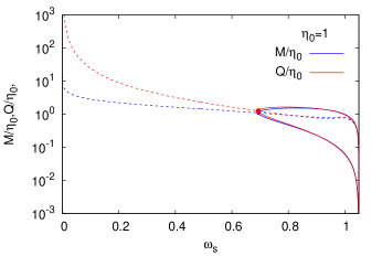
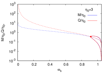
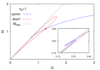
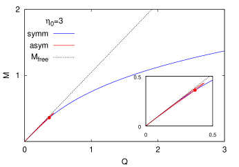
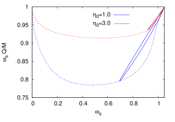
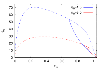
Figure 1: Non-rotating solutions ($n=0$): (a) the scaled mass $M/\eta_{0}$ and the scaled particle number $Q/\eta_{0}$ versus the boson frequency $\omega_{s}$ for throat parameter $\eta_{0}=1$; (b) same as (a) for $\eta_{0}=3$; (c) the mass $M$ versus the particle number $Q$ for throat parameter $\eta_{0}=1$; (d) same as (c) for $\eta_{0}=3$; (e) the quantity $\omega_{s}Q/M$ versus the boson frequency $\omega_{s}$ for throat parameters $\eta_{0}=1$ and $3$; (f) the value of the boson field at the center $\phi_{0}=\phi(0)$ versus the boson frequency $\omega_{s}$ for throat parameters $\eta_{0}=1$ and $3$. The dashed and solid curves correspond to the symmetric and asymmetric solutions, respectively. The dots indicate the bifurcation point of the asymmetric solutions.

We have solved these ordinary differential equations in the full range of the boson frequency $0<\omega_{s}<m_{\rm bs}$, selecting for the throat parameter the values $\eta_{0}=1$ and $3$. In Fig.1 we present the main features of these solutions. Figs.1 and 1 show the mass $M$ and particle number $Q$ versus the boson frequency $\omega_{s}$ for $\eta_{0}=1$ and $\eta_{0}=3$, respectively. Also shown is the mass of $Q$ free particles, $M_{\rm free}=m_{\rm bs}Q$, for comparison.

For large values of the boson frequency $\omega_{s}$ both symmetric and asymmetric solutions exist. As noted above, the latter always appear in pairs, since for any asymmetric solution we obtain a second asymmetric solution by the transformation $\eta\to-\eta$. Then we can consider the three masses shown in the figures as representing the masses of these three solutions at either asymptotically flat region. By going from ${\cal M}_{+}$ to ${\cal M}_{-}$ the masses $M_{+}$ and $M_{-}$ will only be interchanged.

In the limit $\omega_{s}\to m_{\rm bs}$, the mass and particle number tend to zero. In fact, the boson field vanishes in this limit. The limiting solution, then, is the massless Ellis wormhole. Whereas the symmetric solutions extend down to arbitrarily small values of $\omega_{s}$, the asymmetric solutions merge with the symmetric ones at some critical value $\omega_{s}^{\rm cr}$, which depends on $\eta_{0}$, as seen in the figures.

Figs.1 and 1 show the mass as a function of the particle number for the same sets of solutions. We observe that for $\eta_{0}=1$ the mass of the symmetric solutions exhibits two spikes corresponding to three branches of solutions. On the first branch the mass increases with the particle number up to a local maximum. A second branch then extends back to smaller values of the mass and particle number until a local minimum is reached. Here a third branch arises along which the mass increases again monotonically with the particle number. In contrast, for $\eta_{0}=3$ the mass of the symmetric solutions increases monotonically with the particle number, forming only a single branch. For the pair of asymmetric solutions the mass forms a loop, both for $\eta_{0}=1$ and $\eta_{0}=3$. The bifurcation point at $\omega_{s}^{\rm cr}$, where the asymmetric branches end, is indicated by a dot in the figures.

When considering the phenomenon of spontaneous symmetry breaking, observed before in the presence of self-interactions of the boson field Hoffmann:2017jfs , we realize the absence of this phenomenon in the present sets of solutions. While there are symmetric and asymmetric solutions in a certain interval of the parameter space here, as well, we cannot interpret these as arising on energetic grounds. In the case of self-interaction, for a given particle number both asymmetric solutions possess a smaller mass than the symmetric solution. Thus the asymmetric solutions are energetically favoured over the symmetric solutions in the interval where they exist. (Note, that only in the small interval close to $\omega_{\rm max}$ one cannot discern any difference between the three masses.)

In contrast, without the self-interaction present, only the mass of one of the sets of asymmetric solutions is always smaller than the mass of the symmetric solutions for a given particle number. The mass of the other set of asymmetric solutions, however, is larger than the mass of the symmetric solutions for a given particle number in a large range of the interval. In particular, at the bifurcation point the mass of one set of asymmetric solutions approaches the mass of the symmetric solution from below, while the mass of the other set of asymmetric solutions approaches from above.

The energetics of the boson field does not seem to be sufficiently relevant in the present case to give rise to the phenomenon of spontaneous symmetry breaking. Here both symmetric and asymmetric solutions seem to exist, at least in a part of the parameter space, simply because the field equations and the boundary conditions allow for them to exist, when the spacetime topology is non-trivial.

Inspecting Figs.1 and 1 again, we note that in the limit $\omega_{s}\to 0$ the mass and particle number seem to diverge for the symmetric solutions. (The asymmetric ones have ceased to exist below $\omega_{s}^{\rm cr}$.) Remarkably, however, the quantity $\omega_{s}Q/M$ tends to one in this limit, corresponding to $M=\omega_{s}Q+\cdots$, as seen in Fig.1. On the other hand the boson field vanishes as $\omega_{s}\to 0$, as seen in Fig.1, where its central maximal value $\phi_{0}$ is exhibited versus the boson frequency, which seems hard to reconcile with a diverging particle number and mass. To gain some understanding of this limit we will address the behaviour of the solutions in this limit in Appendix B.

III.3 Rotating solutions

We now turn to the rotating solutions. What makes these solutions so special is that the rotation is not imposed via the boundary conditions, as done in the case of the rotating Ellis wormholes Kleihaus:2014dla ; Chew:2016epf . Instead the rotation of the wormholes is generated by the rotation of the bosonic matter into which the wormholes are immersed. This allows for wormhole configurations, where both asymptotically flat regions are completely symmetric Hoffmann:2017vkf . However, besides these symmetric solutions the non-trivial topology allows for asymmetric solutions, as well, as we show below.

We have constructed numerically solutions for the rotational quantum numbers $n=1$ and $n=2$, and for the values of the throat parameter $\eta_{0}=1$ and $\eta_{0}=3$, covering the interval of the boson frequency $0.3\leq\omega_{s}\leq 1.03$. For values of $\omega_{s}$ outside this interval the numerical errors have increased too much, making the solutions no longer fully reliable.

We have solved the system of coupled partial differential equations with the help of the routine FIDISOL/CADSOL schonauer:1989 , a finite difference solver based on a Newton-Raphson scheme. To obtain a finite coordinate patch, we have made a coordinate transformation to a compactified coordinate $x=\arctan(\eta/\eta_{0})$. We have then chosen a non-equidistant grid, employing typically $100\times 40$ grid points in radial direction $x$ and angular direction $\theta$, respectively.

In the following we first consider the global charges of the resulting wormhole solutions. Then we address their ergoregions, their geometry, and their lightrings. We always consider symmetric and asymmetric solutions.

III.3.1 Global charges

        

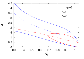
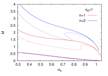
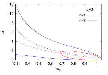
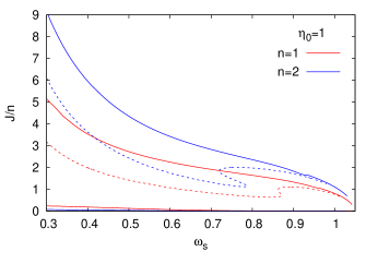
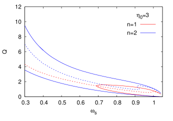
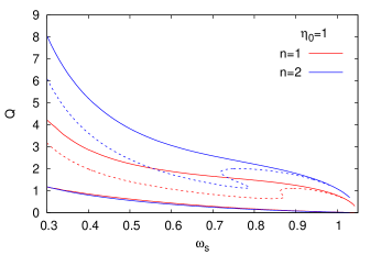
Figure 2: Global charges of rotating solutions: (a) mass $M$ versus boson frequency $\omega_{s}$ for rotational quantum number $n=1$ and $n=2$ for the symmetric (dashed) and asymmetric (solid) solutions for throat parameter $\eta_{0}=3$; (b) same as (a) for $\eta_{0}=1$; (c) scaled angular momentum $J/n$ versus the boson frequency $\omega_{s}$ for rotational quantum number $n=1$ and $n=2$ for the symmetric (dashed) and asymmetric (solid) solutions for throat parameter $\eta_{0}=3$; (d) same as (c) for $\eta_{0}=1$. (e) particle number $Q$ versus the boson frequency $\omega_{s}$ for rotational quantum number $n=1$ and $n=2$ for the symmetric (dashed) and asymmetric (solid) solutions for throat parameter $\eta_{0}=3$; (f) same as (e) for $\eta_{0}=1$.

Let us start our discussion of the wormhole solutions immersed in rotating bosonic matter by addressing their global charges, their mass, angular momentum and particle number. In Fig.2 we show the mass and the angular momentum versus the boson frequency $\omega_{s}$. From Fig.2 we observe that for the smallest (non-trivial) rotational quantum number $n=1$ and throat parameter $\eta_{0}=3$ the situation is analogous to the non-rotating case. The asymmetric solutions exist only down to a critical value of the boson frequency $\omega_{s}^{\rm cr}$, where they bifurcate with the symmetric solutions. The latter again seem to exist in the full interval of the boson frequency.

However, for rotational quantum number $n=2$ and throat parameter $\eta_{0}=3$, we do not observe such a bifurcation of the asymmetric and symmetric solutions any longer. Instead all three sets of solutions, the symmetric one and the pair of asymmetric ones, appear to persist in the full interval of the boson frequency, as seen in the figure. The same holds true for throat parameter $\eta_{0}=1$ and both rotational quantum numbers, $n=1$ and $n=2$, which is illustrated in Fig.2.

Fig.2 and 2 show the angular momentum $J$, scaled by the respective rotational quantum number $n$, for the same sets of solutions. We note, that the scaled angular momentum $J/n$ exhibits a very similar behaviour as the mass of the solutions.

Fig.2 and 2 show the particle number $Q$ computed as outlined in Appendix A for the same sets of solutions. Also the particle number exhibits a very similar behaviour as the mass and the scaled angular momentum of the solutions.

We note, that for the symmetric solutions in Fig.2 additional structures are present, which can be traced back to the presence of a spiral in boson star solutions Jetzer:1991jr ; Lee:1991ax ; Schunck:2003kk ; Liebling:2012fv . This spiral, however, unwinds when a negative energy density is present Dzhunushaliev:2014bya ; Hoffmann:2017jfs ; Hartmann:2013tca . In particular, we observe that backbending of the curves occurs (except for $n=1$ and $\eta_{0}=3$), i.e. mass and angular momentum are then no longer uniquely characterized by the boson frequency $\omega_{s}$. This is in contrast to the asymmetric solutions, where the mass, angular momentum and particle number are unique functions of the boson frequency. In fact, the mass, angular momentum and particle number of all asymmetric solutions decrease monotonically with increasing boson frequency $\omega_{s}$, except for $M_{+}$, $J_{+}$, and $Q_{+}$ for $\eta_{0}=3$ and $n=1$. In the latter case $M_{+}$, $J_{+}$, and $Q_{+}$ possess (local) maxima, but these do not occur at the same value of the boson frequency $\omega_{s}$.

     

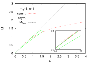
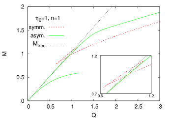
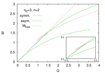
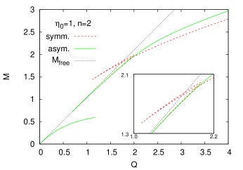
Figure 3: Global charges of rotating solutions: (a) Mass $M$ versus particle number $Q$ for rotational quantum number $n=1$ for the symmetric (dashed) and asymmetric (solid) solutions with throat parameter $\eta_{0}=3$; (b) same as (a) for $\eta_{0}=1$; (c) same as (a) for $n=2$; (d) same as (c) for $\eta_{0}=1$. Also shown is the mass of $Q$ free bosons (thin dotted).

Let us now consider the dependence of the mass on the particle number for these sets of solutions. In Fig.3 we exhibit the mass $M$ versus the particle number $Q$ for rotational quantum number $n=1$ and throat parameter $\eta_{0}=3$ (Fig.3) respectively $\eta_{0}=1$ (Fig.3), as well as for $n=2$, $\eta_{0}=3$ (Fig.3) respectively $\eta_{0}=1$ (Fig.3). Also shown is the mass of $Q$ free particles, $M_{\rm free}=m_{\rm bs}Q$, for comparison.

The case of rotational quantum number $n=1$ and throat parameter $\eta_{0}=3$ (Fig.3) is analogous to the one of the non-rotational case discussed above. Here the set of symmetric solutions forms three branches. On each branch the mass changes monotonically with the particle number. A first branch extends from the vacuum up to some (local) maximum value of the particle number $Q$, where it merges with a second branch, which bends back to some (local) minimum value of $Q$. At this point a third branch arises and extends up to arbitrary large values of $Q$. On the interval where all three branches co-exist the mass is smallest on the first branch and largest on the third branch. The line representing the mass of free particles intersects the second and the third branch. Thus $M<M_{\rm free}$ on the first branch and on the third branch for large enough $Q$, whereas $M>M_{\rm free}$ on most of the second branch and a small part of the third branch.

Let us now turn to the asymmetric solutions. Both $M_{+}(Q_{+})$ and $M_{-}(Q_{-})$ emerge from the vacuum, with $M_{+}\geq M_{-}$. They merge and bifurcate with the symmetric solutions on the third branch of the symmetric solutions. We note that $M_{+}(Q_{+})$ and $M_{-}(Q_{-})$ are smaller than $M_{\rm free}$. Comparing with the mass of the symmetric solutions for some fixed particle number, we note that $M_{-}$ is always the smallest, all the way up to the bifurcation point. $M_{+}$ is smaller than the mass $M$ of the symmetric solutions on the first and on the second branch, although it is remarkably close to the mass $M$ on the first branch. Finally, $M_{+}$ intersects the mass $M$ on the third branch, and exceeds $M$ from the intersection point until the bifurcation point is met.

For small particle number there exist three solutions, a symmetric solution and a pair of asymmetric solutions. In the interval where the second branch of symmetric solutions is present, there are five solutions, three symmetric ones and again a pair of asymmetric solutions. For larger values of the particle number, up to the bifurcation point again three solutions exist. Between the bifurcation point and the maximal value of $Q_{+}$ also three solutions exist. Here, in addition to the symmetric one there are two asymmetric solutions corresponding to two branches of $M_{+}(Q_{+})$. For even larger values of $Q$ only symmetric solutions are present.

Let us now turn to the case $\eta_{0}=1$ and $n=1$ presented in Fig.3. Again the symmetric solutions form three branches. But now the mass is largest on the second branch. The first and the third branch then intersect at a certain value $Q_{\rm int}$. For smaller values of $Q$ the mass is lowest on the first branch, for larger $Q$ it is lowest on the third branch. As in the case of Fig.3 for $\eta_{0}=3$ the line showing the mass of $Q$ free particles intersects the second and the third branch. Since the asymmetric solutions do not bifurcate with the symmetric ones for $\eta_{0}=1$ and $n=1$, $M_{+}$ and $M_{-}$ extend up to arbitrarily large values of $Q$. Both increase monotonically with increasing particle number, and $M_{+}\geq M_{-}$. $M_{+}$ is close to the mass $M$ of the symmetric solutions on the first branch, and exceeds the mass $M$ on the third branch for $Q>Q_{\rm int}$. Similarly to the previous case, for small and large values of $Q$ three solutions are present, while five solutions exist for an intermediate interval.

Now we turn to winding number $n=2$. The case for throat parameter $\eta_{0}=3$ is shown in Fig.3. Starting with the symmetric solutions we observe again three branches. In this case, however, the second branch almost coincides with (part of) the third branch, and can hardly be distinguished in the figure. The asymmetric solutions also behave similarly to the case $\eta_{0}=1$ and $n=1$. Again $M_{+}$ is close to the mass of the symmetric solutions on the first branch, but exceeds the mass on the third branch for sufficiently large values of the particle number. The case $\eta_{0}=3$ and $n=2$ (Fig.3) is qualitatively similar, as well.

We remark, that the phenomenon of spontaneous symmetry breaking remains absent also in the case of rotation. This is not surprising, since the phenomenon is based on a sufficiently strong self-interaction of the boson field, as we have discussed above. If we were to allow for such self-interactions, we would expect this phenomenon to make its reappearance in the presence of rotation.

III.3.2 Ergoregions

     

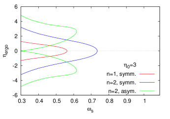
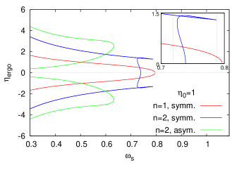
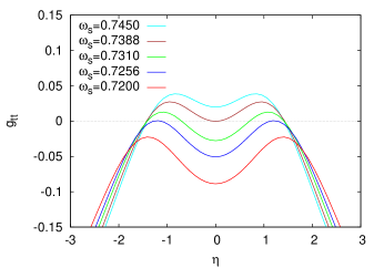
Figure 4: Ergoregion(s) of rotating solutions: (a) the coordinate $\eta_{\rm ergo}$ of the ergosurface(s) in the equatorial plane versus the boson frequency $\omega_{s}$ for rotational quantum number $n=1$ and $n=2$ for the symmetric and asymmetric solutions for throat parameter $\eta_{0}=3$; (b) same as (a) for $\eta_{0}=1$; (c) the metric component $g_{tt}$ in the equatorial plane versus the radial coordinate $\eta$ for throat parameter $\eta_{0}=1$, rotational quantum number $n=2$ and several values of the boson frequency $\omega_{s}$.

We now turn to the ergoregions of the rotating solutions. In Fig.4 we exhibit the coordinate $\eta_{\rm ergo}$ of the ergosurface(s), in the equatorial plane versus the boson frequency $\omega_{s}$ for the same sets of solutions as discussed above. We immediately observe that ergoregions exist only if the boson frequency $\omega_{s}$ is smaller than some maximal value, which depends on the throat parameter $\eta_{0}$, on the rotational quantum number $n$, and on whether the solutions are symmetric or asymmetric.

Let us now consider the ergoregions in more detail, starting with the case of throat parameter $\eta_{0}=3$, shown in Fig.4. We observe that the ergoregions decrease in size with increasing boson frequency $\omega_{s}$, until they degenerate into a circle, when the respective maximal value of $\omega_{s}$ is reached. For the symmetric solutions, this circle then always resides at the throat, i.e., $\eta_{\rm ergo}=0$. For the asymmetric solutions this circle is considerably shifted. But of course there is such a circle for either of the two asymmetric solutions, located symmetrically with respect to each other. We note that the asymmetric solutions for $n=1$, which only exist if $\omega_{s}$ exceeds a critical value, do not possess an ergoregion.

We observe the analogous behaviour for the case of throat parameter $\eta_{0}=1$, shown in Fig.4, except for the symmetric solutions with rotational quantum number $n=2$. This latter case is considerably more involved, because the region where the backbending of the solutions occurs along with its multiple branch structure, resides in this case at sufficiently small values of the boson frequency to fall into the range of frequencies, where ergoregions are present.

Let us therefore look into more detail for this case. Again, at first the ergoregion decreases in size with increasing boson frequency $\omega_{s}$, until the third branch ends, when the second branch begins. On the second branch $\eta_{\rm ergo}$ increases with decreasing $\omega_{s}$, reaches a maximum, and then decreases rapidly. In fact, the ergoregion disappears before the second branch reaches the third branch.

As the boson frequency decreases, in the small interval $0.7256\leq\omega_{s}\leq 0.7388$ the surface of the ergoregion consists of two disconnected parts, each one located on one side of the throat, symmetrically with respect to each other. This is illustrated in Fig.4, where the metric component $g_{tt}$ in the equatorial plane is exhibited versus the radial coordinate $\eta$. At $\omega_{s}=0.7388$, an inner boundary ring appears at the throat, whereas at $\omega_{s}=0.7256$ the ergoregion degenerates into two rings, located symmetrically with respect to each other. Beyond this latter frequency there are no ergoregions found any more along the second branch, and neither along the first branch.

III.3.3 Geometrical properties

        

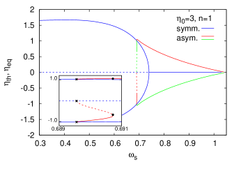
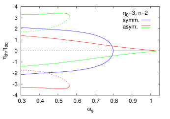
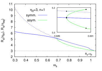
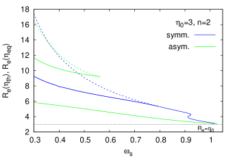
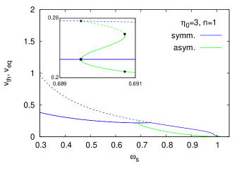
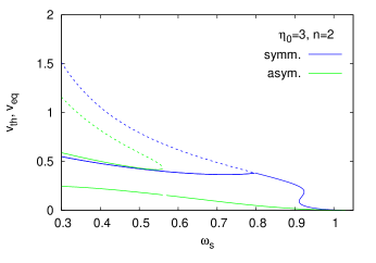
Figure 5: Geometric properties of rotating solutions: (a) the coordinate $\eta_{\rm th}$ of the throat(s) (solid) and the coordinate $\eta_{\rm eq}$ of the equator (dashed) in the equatorial plane versus the boson frequency $\omega_{s}$ for rotational quantum number $n=1$ and throat parameter $\eta_{0}=3$; (b) same as (a) for $n=2$ and $\eta_{0}=3$; (c) the circumferential radius $R_{\rm e}(\eta_{\rm th})$ of the throat(s) (solid) and the circumferential radius $R_{\rm e}(\eta_{\rm eq})$ of the equator (dashed) in the equatorial plane versus the boson frequency $\omega_{s}$ for rotational quantum number $n=1$ and throat parameter $\eta_{0}=3$; The dotted black line indicates the limit $\omega_{s}\to m_{\rm bs}$. (d) same as (c) for $n=2$ and $\eta_{0}=3$; (e) the rotational velocity $v_{\rm th}$ of the throat(s) (solid) and the rotational velocity $v_{\rm eq}$ of the equator (dashed) in the equatorial plane versus the boson frequency $\omega_{s}$ for rotational quantum number $n=1$ and throat parameter $\eta_{0}=3$; (f) same as (e) for $n=2$ and $\eta_{0}=3$.

Let us now address the geometrical properties of the rotating solutions, focusing on the equatorial plane. To this end we present in Fig.5 and Fig.6 the coordinate $\eta_{\rm th}$ of the throat(s), the coordinate $\eta_{\rm eq}$ of the equator when present, the circumferential radius $R_{\rm e}(\eta_{\rm th})$ of the throat(s), the circumferential radius $R_{\rm e}(\eta_{\rm eq})$ of the equator when present, the rotational velocity $v_{\rm th}$ of the throat(s), and the rotational velocity $v_{\rm eq}$ of the equator when present. All quantities are shown versus the boson frequency $\omega_{s}$. Fig.5 exhibits the solutions for throat parameter $\eta_{0}=3$, and Fig.6 those for $\eta_{0}=1$.

        

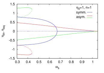
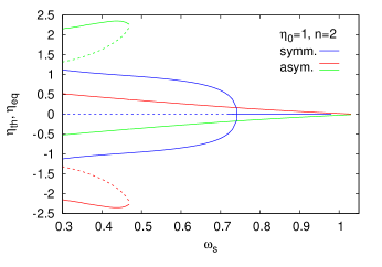
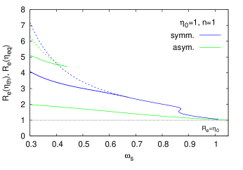
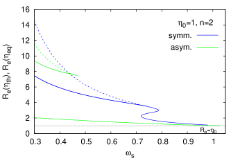
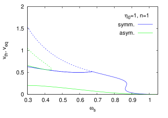
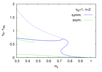
Figure 6: Geometric properties of rotating solutions: (a) the coordinate $\eta_{\rm th}$ of the throat(s) (solid) and the coordinate $\eta_{\rm eq}$ of the equator (dashed) in the equatorial plane versus the boson frequency $\omega_{s}$ for rotational quantum number $n=1$ and throat parameter $\eta_{0}=1$; (b) same as (a) for $n=2$ and $\eta_{0}=1$; (c) the circumferential radius $R_{\rm e}(\eta_{\rm th})$ of the throat(s) (solid) and the circumferential radius $R_{\rm e}(\eta_{\rm eq})$ of the equator (dashed) in the equatorial plane versus the boson frequency $\omega_{s}$ for rotational quantum number $n=1$ and throat parameter $\eta_{0}=1$; The dotted black line indicates the limit $\omega_{s}\to m_{\rm bs}$. (d) same as (c) for $n=2$ and $\eta_{0}=1$; (e) the rotational velocity $v_{\rm th}$ of the throat(s) (solid) and the rotational velocity $v_{\rm eq}$ of the equator (dashed) in the equatorial plane versus the boson frequency $\omega_{s}$ for rotational quantum number $n=1$ and throat parameter $\eta_{0}=1$; (f) same as (e) for $n=2$ and $\eta_{0}=1$.

We start the discussion again with the case of rotational quantum number $n=1$ and throat parameter $\eta_{0}=3$, which features a bifurcation point of the symmetric and asymmetric solutions at a critical boson frequency $\omega_{s}^{\rm cr}$. We observe that for large values of $\omega_{s}$ the wormholes possess only a single throat, until at some particular value of $\omega_{s}$ an equator emerges, as shown in Fig.5. For the symmetric wormholes the throat residing at $\eta=0$ then degenerates into an inflection point. For smaller boson frequency $\omega_{s}$ the circumferential radius $R_{\rm e}$ possesses a maximum at $\eta=0$, corresponding to an equator, while two minima are located symmetrically with respect to $\eta=0$, corresponding to two throats, as demonstrated in Fig.5. Note, that the circumferential radius $R_{\rm e}(\eta_{\rm th})$ of the two throats is of course the same because of symmetry. Therefore only a single solid blue curve is present in Fig.5, also after the equator with circumferential radius $R_{\rm e}(\eta_{\rm eq})$ (dashed blue) has emerged.

Since the asymmetric wormhole solutions always appear in pairs, with one solution related to the other one via reflection symmetry, $\eta\to-\eta$, the asymmetrically located throats of these two solutions are also related via reflection symmetry. To discern them in the figure, the throats of the two solutions are indicated in different colours (red and green). Focusing now on one of the asymmetric solutions only, there is a single throat for large values of the boson frequency $\omega_{s}$. However, at a particular value of the boson frequency, an inflection point emerges on the opposite side of the spacetime, turning into an equator and a second throat as the boson frequency decreases. Note, that these asymmetric wormholes with a double throat exist only in a small region of $\omega_{s}$ close to the bifurcation point $\omega_{s}^{\rm cr}$ with the symmetric solutions. The insets in Fig.5 and Fig.5 highlight this region with double throats. Here the inflection point is indicated by dots, while the bifurcation with the symmetric solutions is indicated by asterisks.

In Fig.5 we demonstrate, that the rotation of the matter is indeed inducing a rotation of the throat(s) and the equator, when present. We therefore exhibit the rotational velocity $v_{\rm th}$ of the throat(s) in the equatorial plane together with the rotational velocity $v_{\rm eq}$ of the equator. We note that for the symmetric solutions the rotational velocity of the center $\eta=0$, representing first a throat and then an equator, increases monotonically with decreasing boson frequency. When the double throat emerges, the rotational velocity of these two symmetrically located throats remains considerably smaller that the rotational velocity of the equator. Concerning the asymmetric solutions we note, that the rotational velocity of the single throat is smallest. The inflection point arises with a higher rotational velocity, with the velocity of the equator increasing and the velocity of the throat decreasing towards the bifurcation point.

In Fig.5 and 5 we present the geometrical properties for throat parameter $\eta_{0}=3$ and rotational quantum number $n=2$. The basic difference is the absence of the bifurcation of the symmetric and asymmetric solutions (at least for $\omega_{s}>0.3$). Thus once the asymmetric solutions develop an equator and a second throat, these features are retained as the boson frequency decreases. Also the geometrical properties of the solutions with the smaller throat parameter $\eta_{0}=1$, shown in Fig.6 are essentially the same as for this case.

     

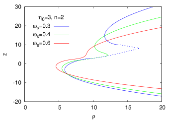
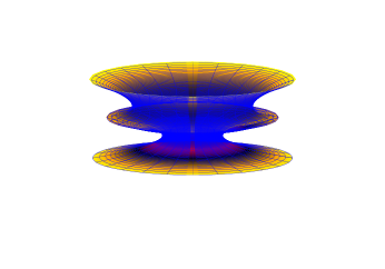
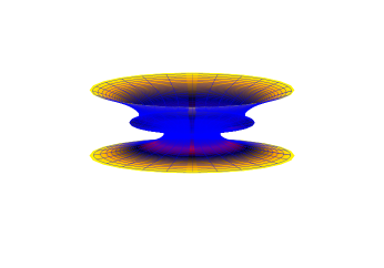
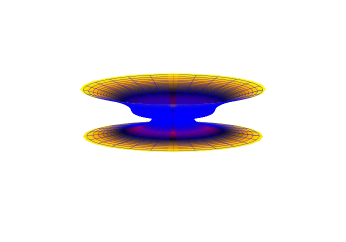
Figure 7: Geometric properties of rotating solutions: embeddings of the equatorial plane of symmetric and asymmetric solutions with throat parameter $\eta_{0}=3$, rotational quantum number $n=2$ and several values of the boson frequency $\omega_{s}$: (a) profile $z(\rho)$ for three embeddings with $\omega_{s}=0.3$, $0.4$ and $0.6$, where a pseudo-euclidean embedding is indicated by dashed lines; (b) 3D plot for $\omega_{s}=0.3$; (c) 3D plot for $\omega_{s}=0.4$; (d) 3D plot for $\omega_{s}=0.6$.

In order to get further insight into the geometry of the wormholes we show in Fig.7 the isometric embedding of the equatorial plane for asymmetric wormhole solutions with throat parameter $\eta_{0}=3$, rotational quantum number $n=2$ and several values of the boson frequency $\omega_{s}$ as examples. Fig.7 exhibits the profile $z(\rho)$ for all three examples, where a pseudo-euclidean embedding is indicated by dashed lines. The remaining figures represent 3-dimensional embeddings, where Fig.7 and Fig.7 correspond to asymmetric double throat solutions ($\omega_{s}=0.3$, resp. $\omega_{s}=0.4$), while Fig.7 represents an asymmetric single throat solution with $\omega_{s}=0.6$.

III.3.4 Lightrings

        

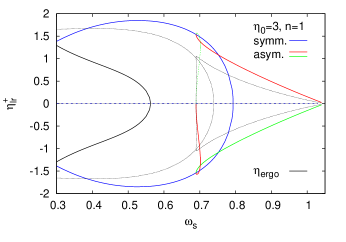
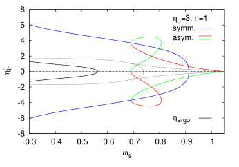
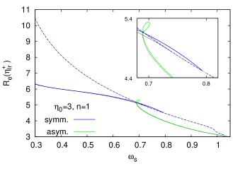
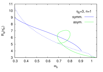
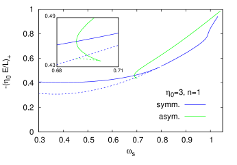
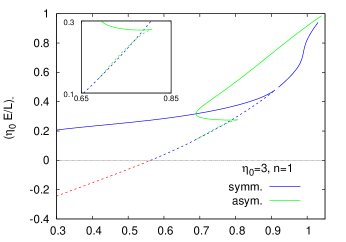
Figure 8: Lightrings of rotating solutions with throat parameter $\eta_{0}=3$ and rotational quantum number $n=1$ versus the boson frequency $\omega_{s}$: (a) the coordinate $\eta^{+}_{\rm lr}$ of co-rotating massless particles in the equatorial plane; (b) the coordinate $\eta^{-}_{\rm lr}$ of counter-rotating massless particles in the equatorial plane; (c) the circumferential radius $R_{\rm e}(\eta^{+}_{\rm lr})$; (d) the circumferential radius $R_{\rm e}(\eta^{-}_{\rm lr})$; (e) the ratio of energy $E$ and angular momentum $L$ of the particle scaled with the throat parameter for co-rotating massless particles; (f) $\eta_{0}E/L$ for counter-rotating massless particles. Also shown are the coordinates and the circumferential radii of the ergosurfaces (black lines).

        

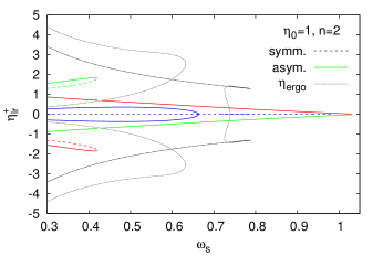
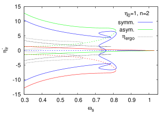
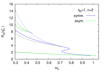
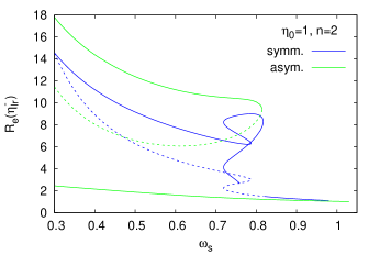
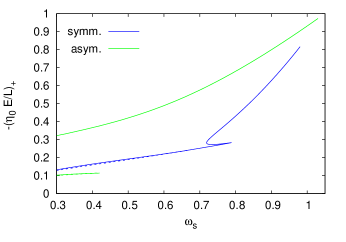
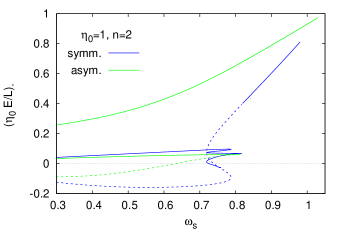
Figure 9: Lightrings of rotating solutions with throat parameter $\eta_{0}=1$ and rotational quantum number $n=2$ versus the boson frequency $\omega_{s}$: (a) the coordinate $\eta^{+}_{\rm lr}$ of co-rotating massless particles in the equatorial plane; (b) the coordinate $\eta^{-}_{\rm lr}$ of counter-rotating massless particles in the equatorial plane; (c) the circumferential radius $R_{\rm e}(\eta^{+}_{\rm lr})$; (d) the circumferential radius $R_{\rm e}(\eta^{-}_{\rm lr})$; (e) the ratio of energy $E$ and angular momentum $L$ of the particle scaled with the throat parameter for co-rotating massless particles; (f) $\eta_{0}E/L$ for counter-rotating massless particles. Also shown are the coordinates and the circumferential radii of the ergosurfaces (black lines).

At last we address the lightrings of these sets of wormhole solutions immersed in rotating bosonic matter. In Fig.8 and Fig.9 we show the properties of the lightrings corresponding to the circular orbits of massless particles in the equatorial plane. Again we begin the discussion with wormhole solutions with throat parameter $\eta_{0}=3$ and rotational quantum number $n=1$, exhibited in Fig.8.

Fig.8 and 8 show the coordinates $\eta^{\pm}_{\rm lr}$, where the lightrings for co-rotating and counter-rotating particles, respectively, are located. For large values of the boson frequency $\omega_{s}$ a single lightring exists for symmetric or asymmetric solutions and both co-rotating or counter-rotating particles. This changes, when the boson frequency reaches a particular value, that depends on the symmetry of the wormhole solutions and the orientation of the orbits. When the boson frequency $\omega_{s}$ becomes smaller than this value, two further lightrings appear. One of the lightrings of the symmetric wormholes is always located at the center $\eta=0$, i.e., either at the throat or at the equator, whereas the other two lightrings are located symmetrically with respect to $\eta=0$ (when present).

In order to discuss the lightrings of the asymmetric wormholes, let us focus on the solution with throat coordinate $\eta_{\rm th}>0$. The lightring which is present already for large values of the boson frequency $\omega_{s}$ is always located outside the throat(s), i.e., $\eta^{\pm}_{\rm lr}>\eta_{\rm th}$. This lightring merges with the lightring of the symmetric wormholes, when the asymmetric and symmetric solutions bifurcate. When $\omega_{s}$ assumes a particular value, a pair of lightrings emerges at some negative coordinate value $\eta^{\pm}_{\rm lc}$ . The inner one of these later merges with the lightring of the symmetric wormhole located at the equator, when the solutions bifurcate. The outer one merges with the corresponding lightring of the symmetric solutions for negative coordinate $\eta$. In the case of counter-rotating massless particles the values of $\omega_{s}$, where multiple lightrings emerge, are larger than in the co-rotating case. Also shown in the figures are the locations of the throat(s) and the equator (dotted black) as well as the ergosurface (solid black).

We show in Fig.8 and 8 the circumferential radii $R_{\rm e}(\eta^{\pm}_{\rm lr})$ of the lightrings for co-rotating and counter-rotating massless particles, respectively. Also shown are the circumferential radii of the throat(s) $R_{\rm e}(\eta^{\pm}_{\rm th})$ and the equator $R_{\rm e}(\eta^{\pm}_{\rm eq})$ (dotted black) for comparison. We note, that the circumferential radii of the lightrings of co-rotating massless particles and the circumferential radii of the throats, respectively the equator, almost coincide, except for those of the pair of lightrings that emerges at the particular value of $\omega_{s}$.

In Fig.8 and 8 we exhibit the ratio of the energy and angular momentum $E/L$, scaled with the throat parameter $\eta_{0}$, for the co-rotating and counter-rotating massless particles, respectively. Since the wormhole spacetime carries negative angular momentum $J$ (by construction), the ratio $E/L$ is negative for co-rotating particles, if we assume positive energy and negative angular momentum $L$. On the other hand, for counter-rotating particles $L$ is then positive. However, as we observe from Fig.8, the ratio $E/L$ of the lightring residing at the equator of the symmetric wormholes becomes negative, when $\omega_{s}$ is smaller than a critical value. Comparison with Fig.8 shows that the change of sign occurs exactly, when the lightring enters the ergosphere.

As a second example we demonstrate the properties of the lightrings for the set of solutions with throat parameter $\eta_{0}=1$ and rotational quantum number $n=2$ in Fig.9. This set is representative for all three sets of solutions, where we do not observe bifurcations of symmetric and asymmetric solutions. Consequently, the new pairs of lightrings persists to smaller boson frequencies, once they have appeared, unless further pairs arise, as in the case of symmetric solutions, where up to five lightrings of counter-rotating massless particles can exist in a certain interval of the boson frequency. Note, that here the branch structure of the solutions complicates the analysis again.

IV Conclusions

We have studied the domain of existence and the physical properties of wormhole solutions immersed in rotating bosonic matter. These solutions arise in General Relativity, when a complex boson field and a phantom field are coupled minimally to gravity. For the complex boson field we have only allowed for a mass term, but not for self-interactions here.

The set of coupled field equations is symmetric with respect to reflection of the radial coordinate, $\eta\to-\eta$. In the presence of rotating matter, the boundary conditions of the metric and the boson field can also be chosen in a symmetric way in both asymptotically flat spacetime regions. Clearly, symmetric solutions then result, where the functions possess reflection symmetry. Interestingly, however, also asymmetric solutions arise in the presence of the non-trivial wormhole topology. However, the reflection symmetry of the system then results in the emergence of pairs of asymmetric solutions, where the two solutions of a pair are related via a reflection transformation, $\eta\to-\eta$.

The complex boson field is characterized by a harmonic time dependence with the boson frequency $\omega_{s}$ and by a rotational quantum number $n$, analogously to the case of $Q$-balls or boson stars. The non-trivial topology of the wormhole spacetime leads, however, to a very different dependence of the solutions on the boson frequency than in the case of boson stars. In particular, the prominent spirals of boson stars have basically unwound, with some backbending of the solutions remaining the only reminder of those spirals.

The absence of self-interactions of the boson field has pronounced consequences. In particular, there are no non-trivial solutions of the boson field in the probe limit. Moreover, the phenomenon of spontaneous symmetry breaking is not present, which is known to occur for non-rotating wormhole solutions, when a sextic self-interaction is included. In that case the masses of both asymmetric solutions are smaller than the mass of the symmetric solution for a given particle number, when the asymmetric solutions bifurcate from the symmetric ones.

Here we have shown that both symmetric and asymmetric solutions can possess an intriguing throat structure. For the symmetric solutions the center is always either a throat or an equator. In the case of an equator the solutions represent double throat solutions, where the throats are located symmetrically on either side of the equator. For the asymmetric solutions the single throat is located asymmetrically with respect to the center, and in the case of double throat solutions, an equator with the second throat emerge on the opposite side of the spacetime. The wormhole solutions can also possess ergoregions, when the rotation is sufficiently fast.

Of interest is also the lightring structure of these spacetimes. Here we have only made a rough first analysis of it, which has revealed that in addition to the single lightring always present further pairs of lightrings can appear. For instance, in the case of counter-rotating particles we have observed the presence of up to five lightrings. A more detailed study of these lightrings and, in particular, of the shadows of these rotating wormhole solutions will be given elsewhere.

Let us briefly address the stability of these wormhole spacetimes immersed in rotating matter. The static Ellis wormholes are known to possess an unstable radial mode Shinkai:2002gv ; Gonzalez:2008wd ; Gonzalez:2008xk ; Torii:2013xba . For rotating wormholes such an analysis is much more involved. However, it has been shown for five-dimensional rotating wormholes, whose two angular momenta have the same magnitude, that this radial instability disappears, when the wormhole throat rotates sufficiently fast Dzhunushaliev:2013jja . This shows that rotation can have a stabilizing effect on the wormhole. Clearly, a stability analysis of these solutions is called for.

Alternatively, one could also consider wormholes in generalized theories of gravity by replacing General Relativity by certain well-motivated gravitational theories, where the phantom field would no longer be needed Hochberg:1990is ; Fukutaka:1989zb ; Ghoroku:1992tz ; Furey:2004rq ; Lobo:2009ip ; Bronnikov:2009az ; Kanti:2011jz ; Kanti:2011yv ; Harko:2013yb , hoping that the instability would disappear along with the phantom field. A study of rotating wormholes in such generalized theories of gravity should be one of our next goals to consider.

Appendix A: Particle number

Here we address the particle number for the asymmetric solutions. We consider the coupling of the complex boson field to an electromagnetic gauge field in the probe limit. Thus we neglect any backreaction of the gauge field to the boson field or the gravitational field. The electromagnetic field is determined from

$$\partial_{\mu}\left(\sqrt{-g}g^{\mu\sigma}g^{\nu\rho}F_{\sigma\rho}\right)=j^{\nu}\sqrt{-g}\ ,$$ (33)

where $F_{\sigma\rho}=\partial_{\sigma}A_{\rho}-\partial_{\rho}A_{\sigma}$ is the field strength of the gauge potenial $A_{\mu}$, and $j^{\nu}$ is the current, i.e.

$$j^{\nu}=-ig^{\nu\mu}\left(\Phi^{*}\partial_{\mu}\Phi-\Phi\partial_{\mu}\Phi^{*}\right)\ .$$ (34)

As ansatz for the gauge potential we choose

$$A_{\mu}dx^{\mu}=a_{0}(\eta,\theta)dt+a_{\varphi}(\eta,\theta)d\varphi\ .$$ (35)

Substitution in the Maxwell equations (33) yields two PDEs for the functions $a_{0}(\eta,\theta)$ and $a_{\varphi}(\eta,\theta)$ to be solved numerically. As boundary conditions we take

$$a_{0}(\pm\infty,\theta)=a_{\varphi}(\pm\infty,\theta)=0\ ,\partial_{\theta}a_{0}(\eta,0)=a_{\varphi}(\eta,0)=0\ ,\partial_{\theta}a_{0}(\eta,\pi/2)=\partial_{\theta}a_{\varphi}(\eta,\pi/2)=0\ .$$ (36)

The charges $Q_{\pm}$ are now determined from the asymptotic behaviour of $a_{0}$,

$$a_{0}\to\pm\frac{Q_{\pm}}{\eta}\ {\rm as}\ \eta\to\pm\infty\ .$$ (37)

Appendix B: Limit $\omega_{s}\to 0$ ($n=0$)

We here address the limit $\omega_{s}\to 0$ of the non-rotating solutions. In Fig.1 we have seen, that both the mass and the particle number seem to diverge as the boson frequency approaches its minimal value, $\omega_{s}\to 0$. At the same time the boson field itself seems to vanish, a fact that appears hard to reconcile with the divergence of mass and particle number. On the other hand, however, we have seem in the figure, that the quantity $\omega_{s}Q/M\to 1$ for $\omega_{s}\to 0$.

     

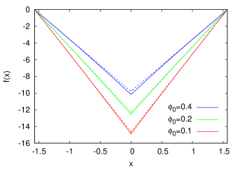
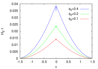
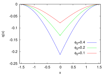
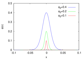
Figure 10: Non-rotating solutions ($n=0$) for throat parameter $\eta_{0}=3$ and central value of the boson field $\phi_{0}=0.4$, $0.2$ and $0.1$: (a) the metric function $f(x)$ versus the compactified radial coordinate $x=\arctan(\eta/\eta_{0})$, the dotted curves show the function $f_{\rm E}(x)$ of the symmetrized Ellis wormholes with the same values of the mass; (b) the relative difference between $f(x)$ and $f_{\rm E}(x)$; (c) the metric function $q(x)$; (d) the boson function $\phi(x)$ close to the center $x=0$.

In order to get some insight into this intriguing situation, let us inspect the behaviour of the solutions in this limit. To this end we exhibit in Fig.10 the metric functions $f$ and $q$ for a sequence of solutions with decreasing central values of the boson field $\phi_{0}$. We observe from Fig.10 that the function $f$ assumes a wedge form whose minimum decreases as $\phi_{0}$ decreases. The dotted lines show the symmetrized massive Ellis wormholes whose metric function reads

$$f_{\rm E}(x)=\frac{2M}{\eta_{0}}\left(|x|-\frac{\pi}{2}\right)\ ,\ \ \ \ \ x=\arctan\left(\frac{\eta}{\eta_{0}}\right)\ ,$$ (38)

and which possess the same mass $M$ as the wormholes immersed in bosonic matter.

Fig.10 shows the relative difference $f(x)/f_{\rm E}(x)-1$. We observe that this difference becomes smaller with decreasing $\phi_{0}$ and seems to vanish as $\phi_{0}\to 0$. On the other hand, we note from Fig.10 that the metric function $q(x)$ vanishes as $\phi_{0}$ tends to zero, which is also consistent with the case of the massive Ellis wormhole. Fig.10 shows the boson field on a small interval around the center $x=0$. We note that the function $\phi(x)$ decreases along with its maximum $\phi_{0}$. At the same time the interval where $\phi(x)$ is noticeably different from zero diminishes with decreasing $\phi_{0}$.

Some insight may come from the field equation of the boson field. For the non-rotating case it reads

$$\left(e^{\frac{q}{2}}h\phi^{\prime}\right)^{\prime}=e^{\frac{3q}{2}-f}\left[m_{\rm bs}^{2}-\omega_{s}^{2}e^{-f}\right]\phi h\ .$$ (39)

Integration from $-\infty$ to $\infty$ yields

$$\left.e^{\frac{q}{2}}h\phi^{\prime}\right|_{-\infty}^{\infty}=\int_{-\infty}^{\infty}{e^{\frac{3q}{2}-f}\left[m_{\rm bs}^{2}-\omega_{s}^{2}e^{-f}\right]\phi h}d\eta\ .$$ (40)

Since the boson field decays exponentially the left hand side vanishes. Consequently, the right hand side also has to vanish. Taking into account that $\phi$ is non-negative, we conclude that the term in the brackets has to change sign. We observe that $f$ assumes its (only) minimum at $\eta=0$, which implies that the term in the brackets also assumes its minimum at $\eta=0$ and is negative there. Thus we arrive at the condition ($f_{0}=f(0)$)

$$m_{\rm bs}^{2}-\omega_{s}^{2}e^{-f_{0}}\leq 0\ \ \ \Longleftrightarrow\ \ \ e^{f_{0}}\leq\frac{\omega_{s}^{2}}{m_{\rm bs}^{2}}\ .$$ (41)

Consequently, we conclude that $f_{0}\to-\infty$ as $\omega_{s}\to 0$.

In Fig.11 we show the ratio $e^{f_{0}}m_{\rm bs}^{2}/\omega_{s}^{2}$ versus the boson frequency $\omega_{s}$ for throat parameters $\eta_{0}=1$ and $3$. We note that this ratio tends to the value one as $\omega_{s}\to 0$. However, in this limit the integrand in Eq. (40) becomes non-negative and solutions cease to exist, except for the case that the boson field $\phi$ vanishes identically.

In Fig.11 we now exhibit the scaled metric function $f(x)/\ln(\omega_{s}^{2}/m_{\rm bs}^{2})$ for throat parameter $\eta_{0}=3$ and decreasing central values of the boson field $\phi_{0}=0.4$, $0.2$, $0.1$ together with the function $1-2|x|/\pi$, which is proportional to the function $f_{\rm E}$ of the symmetrized Ellis wormholes. We note that there is hardly any difference between the functions discernible. In order to illustrate the difference we have to zoom in considerably, as illustrated in the inset of the figure.

     

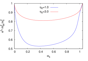
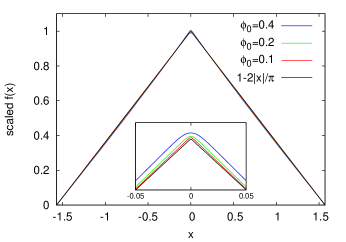
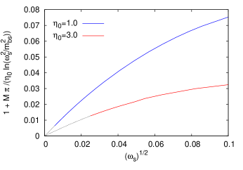
Figure 11: Non-rotating solutions: (a) the ratio $e^{f_{0}}m_{\rm bs}^{2}/\omega_{s}^{2}$ versus the boson frequency $\omega_{s}$ for throat parameter $\eta_{0}=1$ and $3$; (b) the scaled functions $f(x)/\ln(\omega_{s}^{2}/m_{\rm bs}^{2})$ versus the compactified coordinate $x=\arctan(\eta/\eta_{0})$ for throat parameter $\eta_{0}=3$ and central values of the boson field $\phi_{0}=0.4$, $0.2$, $0.1$, also shown is the function $1-2|x|/\pi$; (c) the quantity $1+M\pi/\eta_{0}\ln(\omega_{s}^{2}/m_{\rm bs}^{2})$ versus the square root of the boson frequency $\sqrt{\omega_{s}}$ for throat parameter $\eta_{0}=1$ and $3$ (with thin dotted extrapolation to $\omega_{s}=0$).

Assuming that in the limit $\omega_{s}\to 0$ the metric function behaves like $f(x)=\ln(\omega_{s}^{2}/m_{\rm bs}^{2})(1-2|x|/\pi)$, we conclude that the mass behaves like $M/\eta_{0}=-\ln(\omega_{s}^{2}/m_{\rm bs}^{2})/\pi$. This is demonstrated in Fig.11 where we exhibit the quantity $1+M\pi/\left(\eta_{0}\ln(\omega_{s}^{2}/m_{\rm bs}^{2})\right)$ versus the square root of the boson frequency $\sqrt{\omega_{s}}$ for small values of $\omega_{s}$. For $\omega_{s}\to 0$ this quantity indeed goes to zero.

References

- (1) H. G. Ellis, J. Math. Phys. 14, 104 (1973).
- (2) K. A. Bronnikov, Acta Phys. Polon. B4, 251 (1973).
- (3) T. Kodama, Phys. Rev. D18, 3529 (1978).
- (4) H. G. Ellis, Gen. Rel. Grav. 10, 105 (1979).
- (5) M. S. Morris, K. S. Thorne, Am. J. Phys. 56, 395 (1988).
- (6) M. S. Morris, K. S. Thorne and U. Yurtsever, Phys. Rev. Lett. 61, 1446 (1988).
- (7) F. S. N. Lobo, Phys. Rev. D 71, 084011 (2005).
- (8) F. S. N. Lobo, Fundam. Theor. Phys. 189, pp. (2017).
- (9) V. Dzhunushaliev, V. Folomeev, B. Kleihaus and J. Kunz, JCAP 1104, 031 (2011).
- (10) V. Dzhunushaliev, V. Folomeev, B. Kleihaus and J. Kunz, Phys. Rev. D 85, 124028 (2012).
- (11) V. Dzhunushaliev, V. Folomeev, B. Kleihaus and J. Kunz, Phys. Rev. D 87, 104036 (2013).
- (12) V. Dzhunushaliev, V. Folomeev, B. Kleihaus and J. Kunz, Phys. Rev. D 89, 084018 (2014)
- (13) A. Aringazin, V. Dzhunushaliev, V. Folomeev, B. Kleihaus and J. Kunz, JCAP 1504, 005 (2015).
- (14) V. Dzhunushaliev, V. Folomeev, B. Kleihaus and J. Kunz, JCAP 1608, 030 (2016).
- (15) E. Charalampidis, T. Ioannidou, B. Kleihaus and J. Kunz, Phys. Rev. D 87, 084069 (2013).
- (16) V. Dzhunushaliev, V. Folomeev, C. Hoffmann, B. Kleihaus and J. Kunz, Phys. Rev. D 90, 124038 (2014).
- (17) C. Hoffmann, T. Ioannidou, S. Kahlen, B. Kleihaus and J. Kunz, Phys. Rev. D 95, 084010 (2017).
- (18) C. Hoffmann, T. Ioannidou, S. Kahlen, B. Kleihaus and J. Kunz, Phys. Lett. B 778, 161 (2018).
- (19) P. Jetzer, Phys. Rept. 220, 163 (1992).
- (20) T. D. Lee, Y. Pang, Phys. Rept. 221, 251 (1992).
- (21) F. E. Schunck, E. W. Mielke, Class. Quant. Grav. 20, R301 (2003).
- (22) S. L. Liebling and C. Palenzuela, Living Rev. Rel. 15, 6 (2012).
- (23) P. E. Kashargin and S. V. Sushkov, Grav. Cosmol. 14, 80 (2008).
- (24) P. E. Kashargin and S. V. Sushkov, Phys. Rev. D 78, 064071 (2008).
- (25) B. Kleihaus and J. Kunz, Phys. Rev. D 90, 121503 (2014).
- (26) X. Y. Chew, B. Kleihaus and J. Kunz, Phys. Rev. D 94, 104031 (2016).
- (27) B. Kleihaus and J. Kunz, Fundam. Theor. Phys. 189, 35 (2017).
- (28) F. Abe, Astrophys. J. 725, 787 (2010).
- (29) Y. Toki, T. Kitamura, H. Asada and F. Abe, Astrophys. J. 740, 121 (2011).
- (30) R. Takahashi and H. Asada, Astrophys. J. 768, L16 (2013).
- (31) J. G. Cramer, R. L. Forward, M. S. Morris, M. Visser, G. Benford and G. A. Landis, Phys. Rev. D 51, 3117 (1995).
- (32) M. Safonova, D. F. Torres and G. E. Romero, Phys. Rev. D 65, 023001 (2002).
- (33) V. Perlick, Phys. Rev. D 69, 064017 (2004).
- (34) K. K. Nandi, Y. Z. Zhang and A. V. Zakharov, Phys. Rev. D 74, 024020 (2006).
- (35) K. Nakajima and H. Asada, Phys. Rev. D 85, 107501 (2012).
- (36) N. Tsukamoto, T. Harada and K. Yajima, Phys. Rev. D 86, 104062 (2012).
- (37) P. K. F. Kuhfittig, Eur. Phys. J. C 74, 2818 (2014).
- (38) N. Tsukamoto and T. Harada, Phys. Rev. D 95, 024030 (2017).
- (39) C. Bambi, Phys. Rev. D 87, 107501 (2013).
- (40) P. G. Nedkova, V. K. Tinchev and S. S. Yazadjiev, Phys. Rev. D 88, 124019 (2013).
- (41) M. Zhou, A. Cardenas-Avendano, C. Bambi, B. Kleihaus and J. Kunz, Phys. Rev. D 94, 024036 (2016).
- (42) F. Lamy, E. Gourgoulhon, T. Paumard and F. H. Vincent, arXiv:1802.01635 [gr-qc].
- (43) F. Strocchi, Lect. Notes Phys. 732, 1 (2008).
- (44) F. E. Schunck and E. W. Mielke, in Relativity and Scientific Computing: Computer Algebra, Numerics, Visualization, eds. F. W. Hehl, R. A. Puntigam, and H. Ruder, (Springer Berlin Heidelberg, 1996)
- (45) F. E. Schunck and E. W. Mielke, Phys. Lett. A 249, 389 (1998).
- (46) F. D. Ryan, Phys. Rev. D 55, 6081 (1997).
- (47) S. Yoshida and Y. Eriguchi, Phys. Rev. D 56, 762 (1997).
- (48) F. E. Schunck and E. W. Mielke, Gen. Rel. Grav. 31, 787 (1999).
- (49) B. Kleihaus, J. Kunz and M. List, Phys. Rev. D 72, 064002 (2005).
- (50) B. Kleihaus, J. Kunz, M. List and I. Schaffer, Phys. Rev. D 77, 064025 (2008).
- (51) work in progress.
-
(52)
W. Schönauer and R. Weiß,
J. Comput. Appl. Math. 27, 279 (1989) 279;
M. Schauder, R. Weiß and W. Schönauer, The CADSOL Program Package, Universität Karlsruhe, Interner Bericht Nr. 46/92 (1992). - (53) B. Hartmann, J. Riedel and R. Suciu, Phys. Lett. B 726, 906 (2013).
- (54) H. -a. Shinkai and S. A. Hayward, Phys. Rev. D 66, 044005 (2002).
- (55) J. A. Gonzalez, F. S. Guzman, and O. Sarbach, Class. Quant. Grav. 26, 015011 (2009).
- (56) J. A. Gonzalez, F. S. Guzman, and O. Sarbach, Class. Quant. Grav. 26, 015010 (2009).
- (57) T. Torii and H. a. Shinkai, Phys. Rev. D 88, 064027 (2013).
- (58) V. Dzhunushaliev, V. Folomeev, B. Kleihaus, J. Kunz and E. Radu, Phys. Rev. D 88, 124028 (2013).
- (59) D. Hochberg, Phys. Lett. B251, 349 (1990).
- (60) H. Fukutaka, K. Tanaka, K. Ghoroku, Phys. Lett. B222, 191 (1989).
- (61) K. Ghoroku, T. Soma, Phys. Rev. D46, 1507 (1992).
- (62) N. Furey, A. DeBenedictis, Class. Quant. Grav. 22, 313 (2005).
- (63) F. S. N. Lobo and M. A. Oliveira, Phys. Rev. D 80, 104012 (2009).
- (64) K. A. Bronnikov and E. Elizalde, Phys. Rev. D 81, 044032 (2010).
- (65) P. Kanti, B. Kleihaus and J. Kunz, Phys. Rev. Lett. 107, 271101 (2011).
- (66) P. Kanti, B. Kleihaus and J. Kunz, Phys. Rev. D 85, 044007 (2012).
- (67) T. Harko, F. S. N. Lobo, M. K. Mak and S. V. Sushkov, Phys. Rev. D 87, 067504 (2013).