Proposal for a micromagnetic standard problem for materials with Dzyaloshinskii-Moriya interaction

Abstract

Understanding the role of the Dzyaloshinskii-Moriya interaction (DMI) for the formation of helimagnetic order, as well as the emergence of skyrmions in magnetic systems that lack inversion symmetry, has found increasing interest due to the significant potential for novel spin based technologies. Candidate materials to host skyrmions include those belonging to the B20 group such as FeGe, known for stabilising Bloch-like skyrmions, interfacial systems such as cobalt multilayers or Pd/Fe bilayers on top of Ir(111), known for stabilising Néel-like skyrmions, and, recently, alloys with a crystallographic symmetry where anti-skyrmions are stabilised. Micromagnetic simulations have become a standard approach to aid the design and optimisation of spintronic and magnetic nanodevices and are also applied to the modelling of device applications which make use of skyrmions. Several public domain micromagnetic simulation packages such as OOMMF, MuMax3 and Fidimag already offer implementations of different DMI terms. It is therefore highly desirable to propose a so-called micromagnetic standard problem that would allow one to benchmark and test the different software packages in a similar way as is done for ferromagnetic materials without DMI. Here, we provide a sequence of well-defined and increasingly complex computational problems for magnetic materials with DMI. Our test problems include 1D, 2D and 3D domains, spin wave dynamics in the presence of DMI, and validation of the analytical and numerical solutions including uniform magnetisation, edge tilting, spin waves and skyrmion formation. This set of problems can be used by developers and users of new micromagnetic simulation codes for testing and validation and hence establishing scientific credibility.

I Introduction

In computational science so-called standard problems (or benchmark or test problems) denote a class of problems that are defined in order to test the capability of a newly developed software package to produce scientifically trustworthy results. In the field of micromagnetism which, to a significant extent, relies on results produced by computer simulations, the micromagnetic modeling activity group ($\mathrm{\mu}$mag) at the National Institute of Standards and Technology has helped to define and gather a series of such standard problems for ferromagnetic materials on their website. mumag Those five problems cover static as well as dynamic phenomena and over the years more standard problems have been proposed including the physics of spin transfer torque, Najafi2009 spin waves Venkat2013 and ferromagnetic resonance. Baker2017 Thus far, however, standard problems for materials with Dzyaloshinskii-Moriya interaction (DMI) have not been defined in the literature. Originally, the so-called DMI was phenomenologically described by Dzyaloshinskii Dzyaloshinskii1958 ; Dzyaloshinskii1964 to explain the effect of weak ferromagnetism in antiferromagnets, and later it was theoretically explained by Moriya Moriya1960 as a spin orbit coupling effect. The DMI effect is observable in magnetic materials with broken inversion symmetry and can be present either in the crystallographic structure of the material Bogdanov1989 ; Leonov2015 or at the interface of a ferromagnet with a heavy metal. Crepieux1998 ; Fert2013 ; Wiesendanger2016 In contrast to the favoured parallel alignment of neighbouring spins from the ferromagnetic exchange interaction, the DMI favours the perpendicular alignment of neighbouring spins. The competition between these interactions allow the observation of chiral magnetic configurations such as helices or skyrmions, where spins have a fixed sense of rotation, which is known as chirality.

Skyrmions are localised and topologically non-trivial vortex-like magnetic configurations. Although they were theoretically predicted almost thirty years ago, Bogdanov1989 only recently have skyrmions started to attract significant attention by the scientific community because of multiple recent experimental observations of skyrmion phases in a variety of materials with different DMI mechanisms. Muehlbauer2009 ; Yu2010 ; Milde2013 ; Romming2013 ; Leonov2016 ; Moreau-Luchaire2016 ; Pollard2017 ; Shibata2017 ; Nayak2017 The magnetic profile of a skyrmion changes according to the kind of DMI present in the material. Well-known skyrmionic textures are Néel skyrmions, Bloch skyrmions and anti-skyrmions. Fert2013 ; Wiesendanger2016 ; Nayak2017 ; Hoffmann2017 The former two are named according to the domain wall-like rotation sense of the spins.

The fixed chirality of spins imposed by the DMI causes skyrmions to have different properties from structures such as magnetic bubbles Nagaosa2013 ; Kiselev2011 ; Bernand-Mantel2017 or vortices Butenko2009 ; Mruczkiewicz2017 ; Chen2018 . In addition, the antisymmetric nature of the DMI has an influence on the dynamics of excitations such as spin waves, making them dependent on their propagation direction in the material.

In this paper, we define a set of micromagnetic standard problems for systems with different DMI mechanisms. This set of problems is aimed at verifying the implementation of the DMI by comparing the numerical solutions from different software with semi-analytical results from published studies Rohart2013 ; Bogdanov1994 where possible. In this context, we test these problems using three open-source micromagnetic codes, OOMMF, OOMMFreprt MuMax3 Vansteenkiste2014 and Fidimag. Fidimag In Section III we introduce our analysis by defining the theoretical framework to describe ferromagnetic systems with DMI, which is used to obtain numerical and analytical solutions. Consequently we describe the problems starting by the specification of a one dimensional sample in Section IV, where the DMI has a distinctive influence on the boundary conditions. Then in Section V we test the stabilisation of skyrmionic textures in a disk geometry for different kinds of DMI. In Section VII we compute the spin wave spectrum of an interfacial system in a long stripe and show the antisymmetry produced by the DMI. Finally, in Section VI we analyse a skyrmion in a bulk system, where the propagation of the skyrmion configuration across the thickness of the sample is known to be modulated towards the surfaces because spins acquire an extra radial component. Rybakov2013

II The Dzyaloshinskii-Moriya interaction

The Dzyaloshinskii-Moriya interaction Dzyaloshinskii1958 ; Dzyaloshinskii1964 ; Moriya1960 (DMI) is a spin orbit coupling effect that arises in crystals with a broken inversion symmetry. In these materials the combination of the exchange and spin orbit interactions between electrons leads to an effective interaction between magnetic moments $\mathbf{S}_{i}$ of the form

$$H_{\mathrm{DM}}=\boldsymbol{D}\cdot\left(\boldsymbol{S}_{1}\times\boldsymbol{S}_{2}\right),$$ (1)

where the vector $\boldsymbol{D}$ depends on the induced orbital moments. In general, the DM vector $\boldsymbol{D}$ will be non-zero, although it is strongly constrained via Neumann’s principle, that is, that the Hamiltonian shares (at least) the symmetry of the underlying crystal system. In this context, for two ions it is usually possible to strongly constrain the direction of $\boldsymbol{D}$ through symmetry arguments, such as the ones given in Refs. Yosida1996, ; Moriya1960, . For example, if a mirror plane runs perpendicular to the vector separating two ions, passing through its midpoint, and if the separation is parallel to $z$, then this operation sends $S_{1x}\leftrightarrow S_{2x}$, $S_{1y}\leftrightarrow S_{2y}$, and $S_{1z}\leftrightarrow-S_{2z}$. This means that the transformation causes components proportional only to $D_{z}$ to change signs, forcing $D_{z}$ to vanish but leaving $D_{x}$ and $D_{y}$ nonzero. Yosida1996

When dealing with the continuum (micromagnetic) version of the DMI, the same above considerations apply but may be generalized through the use of a phenomenological approach based on Lifshitz invariants (LIs) Landau1980 ; Bogdanov2002 . Systems featuring LIs range from Chern-Simons terms in gauge field theories, Lancaster2014 to chiral liquid crystals, Sparavigna2009 but also include magnetic systems hosting DMIs. In this latter context they are said to describe inhomogeneous DMIs Bogdanov1989 ; Bogdanov2002 owing to the spatial variation of the magnetization $\mathbf{m}$ that they describe, in the form

$$\mathcal{L}_{ij}^{(k)}=m_{i}\frac{\partial m_{j}}{\partial k}-m_{j}\frac{\partial m_{i}}{\partial k},$$ (2)

where $i,j,k\in\{x,y,z\}$. The precise forms of the LIs are dictated by the crystal symmetry of the system and they determine the micromagnetic expression of its DMI energy. In this continuum limit, the energy written in terms of LIs encodes symmetry constraints elegantly using only a single parameter $D$, by including the way in which the magnetisation (or spin) changes along the different spatial directions. These continuum expressions of the DMI energy are equivalent to the discrete version (equation 1).

The DMI phenomenon also occurs at surfaces Crepieux1998 and in interfacial systems Crepieux1998 ; Bogdanov2001 ; Fert2013 because of the breaking of symmetries. In the latter case, chiral interactions which lead to LIs in the free energy of the system, could arise from broken symmetries reflecting lattice mismatch, defects or interdiffusion between layers Bogdanov2001 . A specific example of this Fert2013 is interfacial DMI arising from the indirect exchange within a triangle composed of two spins and a non-magnetic atom with strong SO coupling. Fert2013 From the atomistic description of interfacial DMI it is possible to derive expressions in the continuum based on LIs as shown in Refs. Yang2015, ; Rohart2013, .

In general, for bulk and interfacial systems the application of the LI-based continuum theory for inhomogeneous DMI, leads to the prediction of a rich variety of non-collinear magnetic structures such as vortex configurations. Bogdanov1989 ; Bogdanov1994 ; Bogdanov2001 ; Leonov2015 An extended discussion on the theory of the DMI and further examples are discussed in Section S1 of the Supplementary Material.

III Analytical model of chiral configurations

For the description of chiral structures in magnetic materials with DMI it is customary to write the magnetisation in spherical coordinates that spatially depend on cylindrical coordinates Bogdanov1994 ; Leonov2015

$$\mathbf{m}=(m_{x},m_{y},m_{z})=(\sin\Theta\cos\Psi,\sin\Theta\sin\Psi,\cos\Theta),$$ (3)

where $(\Theta,\Psi)$ are spherical angles. In the general case, $\Theta=\Theta(r,\phi,z)$ and $\Psi=\Psi(r,\phi,z)$ with $(r,\phi,z)$ being the cylindrical coordinates. In the case of two dimensional systems or magnetic configurations without modulation along the thickness of the sample, $\Theta$ and $\Psi$ are specified independent of the $z$-direction.

For a chiral ferromagnet without inversion symmetry, we are going to describe stable magnetic configurations in confined geometries Rohart2013 when considering symmetric exchange and DMI interactions, an uniaxial anisotropy and in some cases, an applied field. According to this, the energy of the magnetic system is given by

$$E =\int_{V}\text{d}V\,\bigg{(}A\sum_{i\in\{x,y,z\}}(\bm{\nabla}m_{i})^{2}-K_{\text{u}}\left(\mathbf{m}\cdot\hat{z}\right)^{2}$$ (4)

$$\phantom{=\int_{V}\text{d}V\,\bigg{(}}-\mu_{0}\mathbf{M}\cdot\mathbf{H}+w_{\text{DMI}}\bigg{)},$$

where $A$ is the exchange constant, $K_{\text{u}}$ is the uniaxial anisotropy constant, $\mathbf{H}$ the applied field and the last term is the DMI energy density, which can be written as a sum of Lifshitz invariants Bogdanov1989 ; Bogdanov1994 ; Leonov2015 (see Section II). For a material with symmetry class $T$ or $O$, the DMI energy density is specified as

$$w_{\text{DMI}} =D\left(\mathcal{L}_{zy}^{(x)}+\mathcal{L}_{xz}^{(y)}+\mathcal{L}_{yx}^{(z)}\right)$$ (5)

$$=D\mathbf{m}\cdot\left(\bm{\nabla}\times\mathbf{m}\right).$$ (6)

For a thin film with interfacial DMI or a crystal with symmetry class $C_{nv}$, located in the $x-y$ plane, the energy density of the DMI is

$$w_{\text{DMI}} =D\left(\mathcal{L}_{xz}^{(x)}+\mathcal{L}_{yz}^{(y)}\right)$$ (7)

$$=D\left(\mathbf{m}\cdot\bm{\nabla}m_{z}-m_{z}\bm{\nabla}\cdot\mathbf{m}\right).$$ (8)

For a crystal with symmetry class $D_{2d}$, the DMI energy density reads Bogdanov1989

$$w_{\text{DMI}} =D\left(\mathcal{L}_{xz}^{(y)}+\mathcal{L}_{yz}^{(x)}\right)$$ (9)

$$=D\mathbf{m}\cdot\left(\frac{\partial\mathbf{m}}{\partial x}\times\hat{x}-\frac{\partial\mathbf{m}}{\partial y}\times\hat{y}\right).$$ (10)

Axially symmetric magnetic configurations that are uniform along the $z$-direction can be found by substituting the magnetisation $\mathbf{m}$ (equation 3) into equation III, with $\Theta=\Theta(r)$. Accepted solutions for $\Psi$ are obtained according to the structure of the DMI. Bogdanov1989 ; Bogdanov1994 ; Leonov2015 For the $T$ class material, $\Psi=\phi+\varphi$, with $\varphi=0,\pi$. In interfacial systems, the DMI has the structure of a $C_{nv}$ symmetry class material, where $\Psi=\phi+\varphi$ with $\varphi=\pm\pi/2$. For the $D_{2d}$ symmetry class an accepted solution is $\Psi=-\phi+\pi/2$.

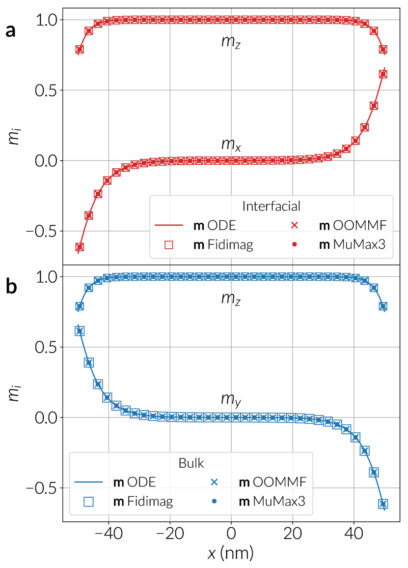
Figure 1: Comparison of the magnetization components along a one-dimensional permalloy-like wire with interfacial (a) or bulk (b) DMI. The wire long axis is specified in the $x$-direction. The plot shows solutions from a theoretical description of the system using an ordinary differential equation (ODE), and solutions from the simulations using the OOMMF, Fidimag and MuMax3 codes.

One-dimensional wire
Dimensions	$100\>\text{nm}\times 1\>\text{nm}\times 1\>\text{nm}$
Magnetic parameters
$A$	$13\>\text{pJ m}^{-1}$
$D$	$3.0\>\text{mJ m}^{-2}$
$M_{\text{s}}$	$0.86\>\text{MA m}^{-1}$
$K_{u}$	$0.4\>\text{MJ m}^{-3}$

Table 1: One-dimensional problem specifications.

IV One-dimensional case: Edge tilting

In a one-dimensional magnetic system in the $x$-direction, where $x\in[0,L]$, and at zero field, we can simplify the expression for the energy (equation III) using $\Theta=\Theta(x)$ and $\phi=0$ (bulk), where $\mathbf{m}=(\sin\Theta,0,\cos\Theta)$, or $\phi=\pi/2$ (interfacial), where $\mathbf{m}=(0,\sin\Theta,\cos\Theta)$. We therefore obtain the following differential equation after minimising the energy with a variational approach Rohart2013

$$\frac{\text{d}^{2}\Theta}{\text{d}x^{2}} =\frac{\sin\Theta\cos\Theta}{\Delta^{2}} \text{for }x(0)<x<x(L)$$

$$\frac{\text{d}\Theta}{\text{d}x} =\pm\frac{1}{\xi} \text{at }x=x(0)\text{ or }x=x(L)$$ (11)

where $\Delta=\sqrt{A/K}$ and $\xi=2A/D$. The positive sign in the boundary condition refers to the interfacial case and the negative sign to the $T$ class material. We solve equations 11 using the shooting method. For this, we refer to the alternative condition for $\Theta$ at $x=0$ or $x=L$ derived in Ref. Rohart2013, , which is valid when the system has a large anisotropy and reads

$$\sin\Theta=\pm\frac{\Delta}{\xi}.$$ (12)

Depending on the chirality of the system, which can be observed from the simulations, we fix the condition $\Theta(0)=\arcsin(\mp\Delta/\xi)$ and vary $\text{d}\Theta(0)/\text{d}x$ until finding a solution that satisfies $\Theta(L)=\arcsin(\pm\Delta/\xi)$. The upper sign $+$ refers to the interfacial case and the bottom sign $-$ to the bulk DMI case.

In Fig. 1a and b we compare results from the theory and simulations of the one dimensional problem, for systems with interfacial ($C_{nv}$) and bulk ($T$) DMI, respectively. For every case we use permalloy-like parameters to test the problem, as specified in Table 1. This material has associated an exchange length of $L_{\text{ex}}=\sqrt{2A/(\mu_{0}M_{\text{s}}^{2})}\approx 5.3\>\text{nm}$ and a helical length of $L_{D}=4\pi A/|D|\approx 54.5\>\text{nm}$. Simulations were performed with the finite difference OOMMF, Fidimag and MuMax3 software. In our examples we used a discretisation cell of $1\times 1\times 1\>\text{nm}^{3}$ volume, whose dimensions are well below the exchange length. The profile of the $z$-component and either the $x$-component of the magnetisation, for the case of interfacial DMI, or the $y$-component for the bulk DMI case, specify the chirality of the magnetic configuration. To obtain the correct chirality in the simulations, the DMI energy expression must be carefully discretised, as explained in the Appendix A. For a one-dimensional system, and since we are using common magnetic parameters, the major difference between the $\mathbf{m}$ profiles of systems with different type of DMI, is the orientation of the spin rotation. Therefore, for a crystal with $T$ or $D_{2d}$ symmetry, the profile of the $m_{y}$ component resemble the $m_{x}$ profile of the interfacial DMI case, which is according to the spin rotation favoured in the $T$ and $D_{2d}$ symmetries. Accordingly, we only show the interfacial and bulk DMI solutions in Fig. 1a and b, respectively. In the plots, data points from the simulations are compared with the solutions of equations 11. In general, OOMMF and Fidimag produce similar results that perfectly agree with the theoretical curves obtained from the solutions of the differential equations (as shown in Fig. 1). Specifically, in the interfacial case the average relative error (between the semi-analytical and simulation curves) for the $m_{x}$ component is about 3.8% and for $m_{z}$ is about 0.3%. Equivalent magnitudes are found for the bulk DMI system. In the case of MuMax3, a similar agreement is found when imposing periodic boundary conditions along the $y$-direction of the one-dimensional system because the DMI calculation is implemented with Neumann boundary conditions Vansteenkiste2014 ; Leliaert2018 rather than free boundaries  (see Section S2 of the Supplementary Material for a comparison when not using periodic boundaries).

V Two-dimensional case: magnetisation profile of a skyrmion

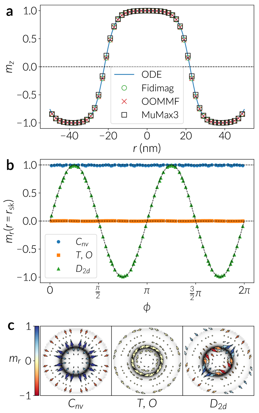
Figure 2: Magnetization profile in permalloy-like disks with three different DMIs from materials with symmetry class $C_{nv}$ (interfacial), $T$ or $O$ (bulk) and $D_{2d}$. (a) Comparison of the out-of-plane component of the magnetization $m_{z}$ from the semi-analytical solution of the ordinary differential equation (ODE) that describes the system, against results from the simulations using three different codes. (b) Radial component of the magnetization in cylindrical coordinates, as a function of the azimuthal angle, computed along the skyrmion radius $r_{\text{sk}}$ (where $m_{z}=0$). The data points shown in the plot were obtained with the Fidimag code and analytical solutions are drawn as thin dashed lines. (c) Snapshots of the disk system for the three different DMI types. Arrows are colored according to the radial component of the magnetization. The background, in grey scale, illustrates the absolute value of the out of plane component of the magnetization, where white means $|m_{z}|=1$ and black means zero. The skyrmion centre is in the $+z$-direction, according to plot (a).

Two-dimensional disk
Radius	$50\>\text{nm}$
Thickness	$2\>\text{nm}$
Magnetic parameters
$A$	$13\>\text{pJ m}^{-1}$
$D$	$3.0\>\text{mJ m}^{-2}$
$M_{\text{s}}$	$0.86\>\text{MA m}^{-1}$
$K_{u}$	$0.4\>\text{MJ m}^{-3}$

Table 2: Two-dimensional problem specifications.

It has been shown in Refs. Carey2016, ; Beg2015, ; Rohart2013, that in a confined geometry spins at the boundary of the system slightly tilt because of the boundary condition and, due to the confinement, skyrmions can be stabilised at zero magnetic field. Experimentally observed skyrmion configurations in materials with three different types of DMIs have been reported in the literature: (i) Interfacial DMI, which favours Néel spin rotations and is equivalent to the DMI found in systems with $C_{nv}$ crystal symmetry. (ii) The so called bulk DMI, which favours Bloch spin rotations and is found in systems with symmetry class $T$ or $O$, such as FeGe. And, recently, (iii) a DMI found in systems with symmetry class $D_{2d}$ where structures known as anti-skyrmions can be stabilised Nayak2017 ; Hoffmann2017 (anti-skyrmions have also been found in interfacial systems but they are best described within a discrete spin formalism Hoffmann2017 ; Camosi2017 ). These three DMI mechanisms can be described by a combination of Lifshitz invariants with a single DMI constant.

We propose a two dimensional cylindrical system of $50\>\text{nm}$ radius and $1\>\text{nm}$ thickness to test the stabilisation of skyrmions using the three aforementioned DMIs, using permalloy-like magnetic parameters as in Section IV (see Table 2).

We summarise in Fig. 2 results obtained for three different skyrmion structures stabilised with the three kind of DMIs. These magnetic configurations were simulated with finite difference codes, as shown in Fig. 2a, which shows a good agreement between them, thus we only plot results from Fidimag in Fig. 2b (see Section S3 in the Supplementary Material for a more detailed comparison). The three skyrmions (see Fig. 2c) are energetically and topologically equivalent, and the magnetization profile depends only on the accepted solution for the $\Psi$ angle when described in spherical coordinates. Therefore, the out of plane component of the spins must match for the three configurations. Solving this system analytically, we can calculate the $\Theta$ angle for the skyrmion solution with the corresponding boundary condition Rohart2013 , by minimising equation III. We compare the out of plane component of the spins, $m_{z}=\cos\Theta$, with that of the simulations by extracting the data from the spins along the disk diameter, which we show in Fig. 2a. As in the one-dimensional case, we observe the characteristic canting of spins at the boundary of the sample.

To distinguish the three different systems, we compute the skyrmion radius $r_{\text{sk}}$ by finding the value of $r$ where $m_{z}(r)=0$, and plot the radial component of the spins $m_{r}$ (see Appendix B) located at a distance $r_{\text{sk}}$ from the disk centre. Since spins are in plane at $r=r_{\text{sk}}$, then $\Theta=\pi/2$ and the radial component (see Appendix B and equation 3) as a function of $\phi$ is $m_{r}(r_{\text{sk}},\phi)=\sin(\Theta(r_{\text{sk}}))\cos(\Psi-\phi)=\cos(\Psi-\phi)$. Therefore, $m_{r_{\mathrm{sk}}}^{C_{nv}}=1$, $m_{r_{\mathrm{sk}}}^{T}=0$ and $m_{r_{\mathrm{sk}}}^{D_{2d}}=\sin(2\phi)$. According to this, we see in Fig. 2b the simulated skyrmion radial profiles at $r=r_{\text{sk}}$ for the $C_{nv}$, $T$ and $D_{2d}$ symmetry class materials, which agree with the theory (shown in dashed lines and curves).

In Fig. 2c we illustrate the three different configurations. The radial component of the magnetisation is shown with a colormap and the out-of-plane component is shown in grayscale, where white means $|m_{z}|=1$, thus it is possible to distinguish the region that defines the skyrmion radius, which is highlighted in black, and the slight spin canting at the disk boundary.

For this two-dimensional problem, the three simulation packages produce similar results and agree well in the solutions, matching the boundary conditions from the theory. The theory predicts a skyrmion radius of $r_{\text{sk}}\approx 22.03\>\text{nm}$. For the calculation of the skyrmion radius in the simulation results, we use a third order spline interpolation of the $m_{z}$ profile from Fig. 2a. According to this, OOMMF and Fidimag give a radius of $21.87\>\text{nm}$ and MuMax3 produces a radius of 22.1 nm, which is a slightly better approximation to the theoretical result.

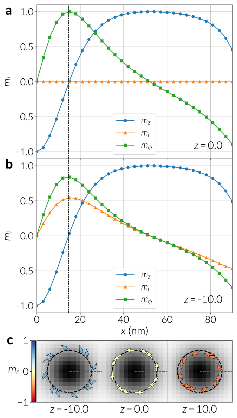
Figure 3: Cylindrical components of the magnetization field of an isolated skyrmion in a FeGe cuboid with periodic boundary conditions. These numerical results were obtained using the Fidimag code. (a) Profiles across the centre of an $x-y$ plane-cut of the cuboid (see red dashed line in snapshots of plot (c)) at $z=0\>\text{nm}$, which is the middle of the sample across the thickness. (b) Profiles at the bottom surface of the cuboid, which is the plane-cut at $z=-10\>\text{nm}$. (c) Snapshots of the magnetization profile at (from left to right) the bottom, middle and top layers of the cuboid (which are plane-cuts) in the $z$-direction. The sample is zoomed at the central region of the layers ($(x,y)\in[-22,22]\>\text{nm}\times[-22,22]\>\text{nm}$) where the skyrmion centre is located. Spins are drawn in a circle defined by the skyrmion radius, which is denoted by a dashed line, and are colored according to their radial component. The background illustrates the out of plane component of the magnetization $m_{z}$, where black means $m_{z}=1$.

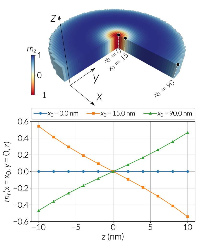
Figure 4: Radial component of the magnetization across the cuboid thickness at three different $(x_{0},y)$ positions for every plane cut in the $z$-direction. The $y$-position is fixed at the centre of the system at $y=0$. The chosen $x$ coordinates are at the centre of the skyrmion ($x_{0}=0$), close to the skyrmion radius ($x_{0}=15\>\text{nm}$), which is approximately 14.9 nm at the sample centre, and at the cuboid periodic boundary ($x_{0}=90\>\text{nm}$). Data points were obtained from Fidimag simulations. The top image shows the cylinder sample under study with the three $(x_{0},y)$ positions marked as dots, and lines denoting where the data is being extracted for every position.

Cylinder
Radius	$90\>\text{nm}$
Thickness	$20\>\text{nm}$
Magnetic parameters
$A$	$8.78\>\text{pJ m}^{-1}$
$D$	$1.58\>\text{mJ m}^{-2}$
$M_{\text{s}}$	$0.384\>\text{MA m}^{-1}$
$\mu_{0}\mathbf{H}$	$(0.0,0.4,0.0)\>\text{T}$

Table 3: Three-dimensional problem specifications.

VI Three-dimensional case: Skyrmion modulation along thickness

Skyrmions hosted in interfacial systems are in general effectively two dimensional structures since these samples are a few monolayers thick. In contrast, in bulk systems skyrmions can form long tubes by propagating their double-twist modulation along their symmetry axis, Buhrandt2013 ; Milde2013 ; Rybakov2013 ; Carey2016 ; Charilaou2017 which we will assume is along the sample thickness. Moreover, it has been shown by Rybakov et al. Rybakov2013 that there is an extra spin modulation along the skyrmion axis that can be approximately described by a linear conical mode solution. This extra modulation is energetically favourable in a range of applied magnetic field and sample thickness values, where the latest is defined below the helix period $L_{D}$. This modulation is greatest at the sample surfaces and is not present at the sample centre along the thickness. It can be identified by an extra radial component acquired by the spins, which is also maximal near the region where $m_{z}=0$ in every slice normal to $z$ (see Fig. 3c).

We define an isolated skyrmion in a FeGe cylinder of $180\>\text{nm}$ diameter and $20\>\text{nm}$ thickness with its long axis (the thickness) in the $z$-direction (see the system illustrated in Fig. 4). We simulate the cylinder using finite differences with cells of $3\>\text{nm}\times 3\>\text{nm}\times 2\>\text{nm}$ volume. Relaxing the system with an initial state resembling a Bloch skyrmion, Beg2015 and an applied magnetic field of $B_{z}=0.4\>\text{T}$, we stabilise a skyrmion tube modulated along the thickness of the sample. A characteristic parameter of FeGe is the helical length $L_{D}=4\pi A/|D|\approx 69.83\>\text{nm}$.

Results from Fidimag simulations are shown in Fig. 3. We obtain a skyrmion tube along the sample thickness with a radius that slightly varies along the $z$-direction (we define as the radius where $m_{z}=0$ in a $x-y$ plane-cut). In a slice of the cylinder at $z=0$, we compute a skyrmion radius of $r_{\text{sk}}\approx 14.9\>\text{nm}$, and this value decreases towards the top and bottom surfaces down to $14.6\>\text{nm}$, which is negligible in the scale of the chosen mesh discretisation. We emphasize that we are not considering the demagnetizing field in this problem, which can enhance this effect.

We analyse the magnetisation field profiles for different slices (different $z$) by plotting the components of the spins located across a layer diameter (or from the skyrmion centre), $(x,y)=(0,0)\>\text{nm}$, up to the sample boundary, $(x,y)=(90,0)\>\text{nm}$, as shown by the red dashed line in every snapshot of Fig. 3c. To quantify the radial modulation of spins, and because of the axial symmetry of skyrmions, we calculate the cylindrical components $m_{r}$ and $m_{\phi}$ (see Appendix B). Consistent with the results of Ref. Rybakov2013, , Fig. 3a reveals that at the middle of the sample, i.e. at the $x-y$ plane-cut located at $z=0$, there is no extra radial component of the spins, which is observed in a two dimensional skyrmion. In addition, due the confined geometry the azimuthal component slightly increases in magnitude towards the sample boundary with an opposite sense of rotation than that of the skyrmion. Towards the sample surfaces, located at $z=\pm 10.0\>\text{nm}$, spins obtain an extra radial component that increases linearly with the $z$ distance. We illustrate this effect in Fig. 3b for the bottom layer at $z=-10.0\>\text{nm}$. Interestingly, the maximum of $m_{r}$ and $m_{\phi}$ are slightly shifted with respect to the $x$-position at $r_{\text{sk}}$, or where $m_{z}(x)=0$, which can be seen from the data points around the dashed line of Fig. 3b. This same effect occurs at the top layer, but with the radial component pointing inwards towards the skyrmion centre, thus $m_{r}$ looks like a mirror image of that of Fig. 3b. Furthermore, we notice that the radial component towards the boundary also changes sign as $m_{\phi}$ does. Snapshots with a zoomed view of the sample for the bottom, middle and top layers are shown in Fig. 3c. We show spins at the skyrmion boundary, where $m_{z}=0$, colored according to their radial component, and with the background colored according to the $m_{z}$ component.

The linear dependence of the radial component $m_{r}$ as a function of $z$ towards the surfaces is shown in Fig. 4, where we plot $m_{r}$ as a function of $z$ at three different $(x,y=0)$ positions in every layer: the centre, $x=0\>\text{nm}$, close to the skyrmion radius $r_{\text{sk}}$ (according to the discretisation of the mesh), $x=15\>\text{nm}$, and at the sample boundary, $x=90\>\text{nm}$. These spatial positions are shown as dots in the cylinder system at the top of Fig. 4, with lines denoting where the data is being extracted. From the curves of Fig. 4 we notice that the radial increment is maximal close to the skyrmion radius and is slightly smaller, and with opposite orientation, at the cylinder boundary normal to the radial direction.

Our results show that the skyrmion at the $z=0$ slice does not have a radial modulation and the skyrmion size remains nearly constant across the sample thickness. Hence, it would be possible to use a two-dimensional model, similar to the one used in Sections III and V, to describe its profile. In performing this comparison (see Section S4 in the Supplementary Material) we noticed that the skyrmion in the cylinder system has a larger skyrmion radius than the model predicts. In Ref. Rybakov2013, an approximate solution is provided as an ansatz for the $\Psi$ angle, which is based on a linear dependence on $z$. Although this approximation qualitatively describes the effects observed from the simulations, a more accurate solution would be possible to obtain by taking the general case $\Theta=\Theta(r,z)$ and $\Psi=\Psi(\phi,z)$, but it generates a non-trivial set of non-linear equations to be minimised. Because of the consistent skyrmion size across $z$ it is likely that the dependence on $z$ in the $\Theta$ angle only appears as a weak term or a constant, which differentiates the solution from that of the two-dimensional model.

Testing this problem using the OOMMF code we obtain equivalent results with the same skyrmion radius size. In the case of MuMax3, we had to use a slightly different mesh discretisation, since the software only accepts an even number of cells, which we adjusted to get a similar sample size. Results from MuMax3 simulations produce a skyrmion with larger radii compared to Fidimag and OOMMF, with magnitudes of approximately 15.9 nm close to $z=0$ and 15.6 nm at the cylinder caps. Nevertheless, the tendencies of the radial profiles of the magnetisation are still close to the ones obtained with the other codes. Details of these simulations are provided in Section S5 of the Supplementary Material. Although a cylinder system is also suitable for finite element code simulations, a cuboid geometry is more natural to a finite difference discretisation. Hence, we performed a similar study using a cuboid with periodic boundary conditions. In general results on this geometry are equivalent to the cylinder but with two main differences: the periodicity removes the effects at the boundaries and the skyrmion is slightly larger in radius. These solutions are shown in Section S6 of the Supplementary Material.

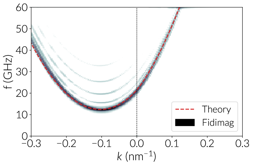
Figure 5: Spectrum of Damon-Eshbach spin waves in a permalloy-like stripe with interfacial DMI. The theoretical curve is computed from the theory of Moon et al. Moon2013 and the intensity plot refers to the result of the computer simulation of the system using the Fidimag code. The intensity plot is given in logarithmic scale.

VII Dynamics: asymmetric spin wave propagation in the presence of DMI

Analyzing the dynamics of a magnetic system is a standard method to obtain information about the magnetic properties of the material, such as damping or the excitation modes of the system, among others. In particular, it is known that the spin wave spectrum of a material with DMI saturated with an external bias field, is antisymmetric along specific directions where spin waves are propagating. Cortes-Ortuno2013 ; Moon2013 These directions depend on the nature of the DMI, and from the antisymmetry it is possible to quantify a frequency shift from modes with the same wave vector magnitude but opposite orientation, i.e. from waves travelling in opposite directions. This frequency shift depends linearly on the DMI magnitude of the material and hence it is a straightforward method for measuring this magnetic parameter. This has been proved in multiple experiments based on Brillouin light scattering. Belmeguenai2015 ; Di2015 ; Tacchi2017 Accordingly, a standard problem based on spin waves offers the possibility to test the DMI influence on the spin dynamics of the system.

Two-dimensional stripe
Dimensions	$2000\>\text{nm}\times 200\>\text{nm}\times 1\>\text{nm}$
Magnetic parameters
$A$	$13\>\text{pJ m}^{-1}$
$D$	$3.0\>\text{mJ m}^{-2}$
$M_{\text{s}}$	$0.86\>\text{MA m}^{-1}$
$\mu_{0}\mathbf{H}$	$(0.0,0.4,0.0)\>\text{T}$
$\mu_{0}\mathbf{h}_{\text{exc}}$	$(0.04,0.0,0.0)\>\text{T}$
$f_{0}$	$60\>\text{GHz}$
$t_{0}$	$50\>\text{ps}$
$\gamma$	$2.21\times 10^{5}\>\text{Hz T}^{-1}$
$\alpha$	$0.01$
$\tau$	$4\>\text{ns}$
$\Delta\tau$	$1\>\text{ps}$

Table 4: Spin wave problem specifications.

In interfacial systems spin waves propagating perpendicular to a saturating bias field, which are known as Damon-Eshbach modes, exhibit antisymmetric behaviour. Cortes-Ortuno2013 ; Moon2013 To simulate this phenomenon, we refer to the method specified in Ref. Venkat2013, and use values from Table 4,

1. Define a thin stripe with the long axis in the $x$-direction and thickness along the $z$-direction.

2. Saturate and relax the sample using a sufficiently strong bias magnetic field. If the relaxation is done with the LLG equation it is possible to remove the precessional term and use a large damping to accelerate the relaxation.

3. Excite the system with a weak periodic field, based on a sinc function, in a small region at the centre of the stripe and applied in a specific direction $\hat{x}_{i}$,

   $$\mathbf{h}_{\text{exc}}=h\,\text{sinc}\left(2\pi f_{0}(t-t_{0})\right)\hat{x}_{i}.$$ (13)

   We delay this signal by $t_{0}$, and then excite the system during the time $\tau$, saving the magnetization field every interval of duration $\Delta\tau$.

4. Using the magnetization field files, we extract the dynamic components of the magnetization for a chain of magnetic moments along the $x$-direction across the middle of the stripe. The dynamic component is obtained by subtracting, from the excited spins, the components of the magnetic moments of the relaxed state obtained in step 2.

5. We save these components in a matrix, where every column is a magnetization component, $m_{x},m_{y}$ or $m_{z}$, of the spins across the spatial $x$-direction, and every row represents a saved time step saved in the previous step.

6. Perform a two-dimensional spatial-temporal Fourier transform of the matrix, applying a Hanning windowing function Kumar2012 .

We define a permalloy stripe, with magnetic parameters specified in Table 4, saturating the magnetization into the $y$-direction. For this sample we take into account dipolar interactions. To obtain a spectrum for positive and negative wave vectors, i.e., for waves propagating in opposite directions, we excite the system in a small region of $2\>\text{nm}$ width at the centre of the stripe, with a weak periodic signal based on the cardinal sine wave function. We excite Damon-Eshbach spin waves by applying the sinc field in the $x$-direction for a duration of $\tau=4\>$ns. According to Table 4 we save $\tau/\Delta\tau=4000$ steps to generate the spin wave spectrum.

The result of the spin waves simulation using Fidimag, after processing the data, is shown in Fig. 5. In the spectrum we compare the result using the theory of Moon et al. Moon2013 for systems with interfacial DMI. The asymmetry in the spin wave depends on the DMI sign. To compare the theoretical curve with the data from the simulations we calculated the minimum in the dispersion relation for both curves. For the simulations we calculated the peaks with largest intensity from the spectrum and fit the data with a fourth order polynomial. The theory predicts that the minimum is located at $k=-0.1036\>\text{nm}^{-1}$ with a frequency of $12.4098\>\text{GHz}$. From the Fidimag simulation we estimate the minimum at $k=-0.1007\>\text{nm}^{-1}$ and $f=12.1690\>\text{GHz}$, which shows they are in good agreement. As an extra test we can notice from Ref. Cortes-Ortuno2013, that in systems with crystallographic classes $T$ or $D_{2d}$, the Damon-Eshbach spin waves will not be antisymmetric, however they would be for spin waves excited along the field direction.

In Fig. 5 we observe the presence of extra modes with a smaller intensity signal. These modes can be filtered by setting an exponential damping towards the boundaries of the stripe Venkat2018 to avoid the reflection of spin waves. In the codes provided in the manuscript we implemented functions for the damping with a simple exponential profile that can be used to only obtain the main branch from the spectrum.

Using the OOMMF and MuMax3 codes for simulating spin waves in systems with DMI produced equivalent results to Fig. 5. With OOMMF simulations we obtained a minimum at $k=-0.1001\>\text{nm}^{-1}$ and $f=12.1796\>\text{GHz}$, while simulations performed with MuMax3 produce values of $k=-0.1014\>\text{nm}^{-1}$ and $f=12.5232\>\text{GHz}$, which is a slightly better approximation. Results for OOMMF and MuMax3 simulations, and details about the numerical interpolation to the curves are shown in Section S7 of the Supplementary Material.

VIII Conclusions

We have proposed four standard problems to validate the implementation of simulations of helimagnetic systems with DMI mechanisms found in crystals with $C_{nv}$, $T$ and $D_{2d}$ symmetry class, where the former is also relevant in interfacial systems. The strength of the three DMI types we use in the problems can be quantified by a single DMI constant. For the one-dimensional and two-dimensional problems we test the boundary condition in confined geometries, which can be compared with analytical solutions. Moreover, profiles of different skyrmionic textures, which vary according to the DMI kind, are characterised by their radial profile, in particular at a distance $r$ from the skyrmion centre where $m_{z}=0$, which we define as the skyrmion radius. Further, in order to test the effect of the DMI on the dynamics of the systems, we propose a problem based on the excitation of spin waves and the calculation of their spectrum. In this case, we analyse Damon-Eshbach spin waves in a stripe with interfacial DMI (or, equivalently, a crystal with $C_{nv}$ symmetry), which is known for being antisymmetric, and compare the solution with analytical theory. Finally, we analyse an isolated skyrmion in a bulk material with symmetry class $T$ in a cylinder. In this sample the skyrmion profile propagates through the thickness and acquires an extra radial modulation. We notice that this modulation is non-existent in a slice at the middle of the sample along the thickness direction and increases linearly towards the cylinder caps (normal to the $z$-direction). Additionally, it is greatest at the skyrmion radius (where $m_{z}=0$), decreases to zero at the skyrmion centre and towards the skyrmion boundary (in every slice), and is present at the cylinder boundary (normal to the radial direction) with an opposite orientation than the one within the skyrmion configuration.

Simulations in this study have been performed using codes based on the finite difference numerical technique. Since many of the problems are compared with semi-analytical calculations the results can be also applied to finite element code simulations. Some finite element computations with our non-publicly available software Finmag are shown in Section S8 of the Supplementary Material. In addition, we compared our data with the results from a non-public finite-element code developed by R. Hertel, which is an entirely rewritten successor of the TetraMag software Hertel2007a ; Kakay2010 . These results are also shown in Section S8, where we obtained an excellent quantitative agreement.

With this set of problems we intend to cover the functionality of the DMI interaction implemented in a micromagnetic code by testing boundary conditions, energy minimisation, which can be achieved using LLG dynamics or minimisation algorithms such as the conjugate gradient method, and spin dynamics. Overall, the micromagnetic codes used in our testings significantly agree with expected solutions and comparisons with the theory, thus our results substantiate studies based on micromagnetic simulations with the three codes we have tested. We hope this systematic analysis helps to promote the publication of codes in simulation based studies for their corresponding validation and reproducibility, and serve as a basis for more effective development of new simulation software.

For the realisation of some of the problems, we have implemented new DMI modules for MuMax3 Cortes2018 and OOMMF OOMMFa ; OOMMFb ; OOMMFc ; Cortes2018 that take advantage of the computer softwares framework, such as GPU implementation in MuMax3 or the robustness of OOMMF. We have used the Jupyter OOMMF (JOOMMF) interface to drive OOMMF and analyse data. JOOMMF2017 . Scripts and notebooks to reproduce the problems and data analysis from this paper can be found in Ref. Cortes2018, .

Appendix A Finite difference discretisation for the DMI

Assuming a two dimensional film positioned in the $x-y$ plane, the energy density $w$ for the interfacial DMI used in this study is modeled as

$$w_{\text{DMI}} =D\left(\mathcal{L}_{xz}^{(x)}+\mathcal{L}_{yz}^{(y)}\right)$$ (14)

$$=D\left(m_{x}\frac{\partial m_{z}}{\partial x}-m_{z}\frac{\partial m_{x}}{\partial x}+m_{y}\frac{\partial m_{z}}{\partial y}-m_{z}\frac{\partial m_{y}}{\partial y}\right).$$ (15)

The corresponding effective field of this interaction reads

$$\mathbf{H}_{\text{DMI}} =-\frac{1}{\mu_{0}M_{s}}\frac{\delta w_{\text{DMI}}}{\delta\mathbf{m}}$$ (16)

$$=-\frac{2D}{\mu_{0}M_{s}}\left(\frac{\partial m_{z}}{\partial x}\hat{x}+\frac{\partial m_{z}}{\partial y}\hat{y}-\left[\frac{\partial m_{x}}{\partial x}+\frac{\partial m_{y}}{\partial y}\right]\hat{z}\right).$$ (17)

When using finite differences, we can discretise the derivatives using a central difference at every mesh site. Thus, for example, the central difference for the first derivative of $m_{z}$ with respect to $x$ is

$$\frac{\partial m_{z}}{\partial x}\approx\frac{m_{z}(+x)-m_{z}(-x)}{2\Delta x},$$ (18)

where $m_{z}(\pm x)$ is the $m_{z}$ component of the closest magnetic moment at the mesh site in the $\pm x$-direction and $\Delta x$ is the mesh discretisation in the $x$-direction. We can then, for every mesh site, collect all the terms related to the contribution to the field from its 4 mesh neighbours in the plane where the system is defined. For instance, the field contribution from the $+x$ mesh neighbour is

$$\mathbf{h}_{\text{DMI}}(+x) =-\frac{2D}{\mu_{0}M_{s}}\frac{1}{2\Delta x}\left(m_{z}(+x)\hat{x}-m_{x}(+x)\hat{z}\right)$$ (19)

$$=-\frac{2D}{\mu_{0}M_{s}}\frac{1}{2\Delta x}\left(\left[\hat{z}\times\hat{x}\right]\times\mathbf{m}(+x)\right).$$ (20)

The contribution for the other neighbours have the same structure except the denominator for the neighbours in the $y$-direction will have a factor of $2\Delta y$ instead of $2\Delta x$ (similar for $z$). In addition, the cross product is, in general, given by $(\hat{z}\times\hat{r}_{ij})\times\mathbf{m}$, with $\hat{r}_{ij}$ the unit vector from the $i$ mesh site directed towards the neighbour in the $j$-direction. Hence, the calculation for the field is similar than that of the Heisenberg-like model, with an equivalent DMI vector of the form $(\hat{z}\times\hat{r}_{ij})$.

It is important to mention that an interfacial DMI described within the discrete spin model using the DMI vector $\mathbf{D}_{ij}=(\hat{r}_{ij}\times\hat{z})$, in the continuum limit leads to expression 15. However, when using finite differences for the continuum description of the system, the calculation of the field related to equation 15, which is similar to the atomistic model calculation, has an opposite sign for the equivalent DMI vector.

Similarly, for a $T$ class material, the finite differences discretisation leads to a calculation of the micromagnetic DMI field using a vector $\hat{r}_{ij}$. In the case of $D_{2d}$ symmetry, this vector is $-\hat{r}_{ij}$ in the $x$-directions and $\hat{r}_{ij}$ in the $y$-directions.

Appendix B Cylindrical components

The cylindrical components of the magnetization are computed with a transformation matrix according to

$$\begin{bmatrix}\cos\phi&\sin\phi&0\\ -\sin\phi&\cos\phi&0\\ 0&0&1\\ \end{bmatrix}\begin{bmatrix}m_{x}\\ m_{y}\\ m_{z}\\ \end{bmatrix}=\begin{bmatrix}m_{r}\\ m_{\phi}\\ m_{z}\\ \end{bmatrix}$$ (21)

where $\phi=\arctan(y/x)$ is the azimuthal angle.

See pages 1 of SupplementaryMaterial.pdf See pages 2 of SupplementaryMaterial.pdf See pages 3 of SupplementaryMaterial.pdf See pages 4 of SupplementaryMaterial.pdf See pages 5 of SupplementaryMaterial.pdf See pages 6 of SupplementaryMaterial.pdf See pages 7 of SupplementaryMaterial.pdf See pages 8 of SupplementaryMaterial.pdf See pages 9 of SupplementaryMaterial.pdf See pages 10 of SupplementaryMaterial.pdf See pages 11 of SupplementaryMaterial.pdf See pages 12 of SupplementaryMaterial.pdf See pages 13 of SupplementaryMaterial.pdf See pages 14 of SupplementaryMaterial.pdf See pages 15 of SupplementaryMaterial.pdf See pages 16 of SupplementaryMaterial.pdf See pages 17 of SupplementaryMaterial.pdf See pages 18 of SupplementaryMaterial.pdf See pages 19 of SupplementaryMaterial.pdf

References

- (1) http://www.ctcms.nist.gov/ rdm/mumag.org.html.
- (2) Najafi, M. et al. Proposal for a standard problem for micromagnetic simulations including spin-transfer torque. J. Appl. Phys. 105, 113914 (2009).
- (3) Venkat, G. et al. Proposal for a Standard Micromagnetic Problem: Spin Wave Dispersion in a Magnonic Waveguide. IEEE Trans. Magn. 49, 524–529 (2013).
- (4) Baker, A. et al. Proposal of a micromagnetic standard problem for ferromagnetic resonance simulations. J. Magn. Magn. Mater. 421, 428 – 439 (2017).
- (5) Dzyaloshinskii, I. A thermodynamic theory of “weak” ferromagnetism of antiferromagnetics. J. Phys. Chem. Solids 4, 241–255 (1958).
- (6) Dzyaloshinskii, I. E. Theory of helicoidal structures in antiferromagnets. II. Metals. Soviet Physics JETP 19, 960–971 (1964).
- (7) Moriya, T. Anisotropic superexchange interaction and weak ferromagnetism. Phys. Rev. 120, 91–98 (1960).
- (8) Bogdanov, A. & Yablonskii, D. Thermodynamically stable ”vortices“ in magnetically ordered crystals. The mixed state of magnets. Zh. Eksp. Teor. Fiz 95, 178 (1989).
- (9) Leonov, A. O. et al. The properties of isolated chiral skyrmions in thin magnetic films. New J. Phys. 18, 1–12 (2015).
- (10) Crépieux, A. & Lacroix, C. Dzyaloshinsky-Moriya interactions induced by symmetry breaking at a surface. J. Magn. Magn. Mater. 182, 341–349 (1998).
- (11) Fert, A., Cros, V. & Sampaio, J. Skyrmions on the track. Nat. Nanotechnol. 8, 152–156 (2013).
- (12) Wiesendanger, R. Nanoscale magnetic skyrmions in metallic films and multilayers: a new twist for spintronics. Nature Reviews Materials 1, 16044 (2016).
- (13) Mühlbauer, S. et al. Skyrmion lattice in a chiral magnet. Science 323, 915–919 (2009).
- (14) Yu, X. Z. et al. Real-space observation of a two-dimensional skyrmion crystal. Nature 465, 901–904 (2010).
- (15) Milde, P. et al. Unwinding of a Skyrmion Lattice by Magnetic Monopoles. Science 340, 1076–1080 (2013).
- (16) Romming, N. et al. Writing and Deleting Single Magnetic Skyrmions. Science 341, 636–639 (2013).
- (17) Leonov, A. O. et al. Chiral Surface Twists and Skyrmion Stability in Nanolayers of Cubic Helimagnets. Phys. Rev. Lett. 117, 087202 (2016).
- (18) Moreau-Luchaire, C. et al. Additive interfacial chiral interaction in multilayers for stabilization of small individual skyrmions at room temperature. Nat. Nanotechnol. 11, 444–448 (2016).
- (19) Pollard, S. D. et al. Observation of stable Néel skyrmions in cobalt/palladium multilayers with Lorentz transmission electron microscopy. Nat. Commun. 8 (2017).
- (20) Shibata, K. et al. Temperature and Magnetic Field Dependence of the Internal and Lattice Structures of Skyrmions by Off-Axis Electron Holography. Phys. Rev. Lett. 118, 087202 (2017).
- (21) Nayak, A. K. et al. Magnetic antiskyrmions above room temperature in tetragonal Heusler materials. Nature 548, 561–566 (2017).
- (22) Hoffmann, M. et al. Antiskyrmions stabilized at interfaces by anisotropic Dzyaloshinskii-Moriya interactions. Nat. Commun. 8, 308 (2017).
- (23) Nagaosa, N. & Tokura, Y. Topological properties and dynamics of magnetic skyrmions. Nat. Nanotechnol. 8, 899–911 (2013).
- (24) Kiselev, N. S., Bogdanov, A. N., Schäfer, R. & Rößler, U. K. Chiral skyrmions in thin magnetic films: new objects for magnetic storage technologies? J. Phys. D: Appl. Phys. 44, 392001 (2011).
- (25) Bernand-Mantel, A. et al. The skyrmion-bubble transition in a ferromagnetic thin film. ArXiv e-prints (2017). eprint 1712.03154.
- (26) Butenko, A. B., Leonov, A. A., Bogdanov, A. N. & Rößler, U. K. Theory of vortex states in magnetic nanodisks with induced Dzyaloshinskii-Moriya interactions. Phys. Rev. B 80, 134410 (2009).
- (27) Mruczkiewicz, M., Krawczyk, M. & Guslienko, K. Y. Spin excitation spectrum in a magnetic nanodot with continuous transitions between the vortex, Bloch-type skyrmion, and Néel-type skyrmion states. Phys. Rev. B 95, 094414 (2017).
- (28) fu Chen, Y. et al. Nonlinear gyrotropic motion of skyrmion in a magnetic nanodisk. J. Magn. Magn. Mater. – (2018).
- (29) Rohart, S. & Thiaville, A. Skyrmion confinement in ultrathin film nanostructures in the presence of Dzyaloshinskii-Moriya interaction. Phys. Rev. B 88, 184422 (2013).
- (30) Bogdanov, A. & Hubert, A. The properties of isolated magnetic vortices. Phys. Status Solidi B 186, 527–543 (1994).
- (31) Donahue, M. J. & Porter, D. G. OOMMF User’s Guide, Version 1.0. Tech. Rep., National Institute of Standards and Technology, Gaithersburg, MD (1999).
- (32) Vansteenkiste, A. et al. The design and verification of MuMax3. AIP Adv. 4, 107133 (2014).
- (33) Cortés-Ortuño, D. et al. Fidimag. Zenodo doi:10.5281/zenodo.594647. Github: https://github.com/computationalmodelling/fidimag/ (2018).
- (34) Rybakov, F., Borisov, A. & Bogdanov, A. Three-dimensional skyrmion states in thin films of cubic helimagnets. Phys. Rev. B 87, 094424 (2013).
- (35) Yosida, K. Theory of Magnetism, vol. 122 of Springer Ser. Solid-State Sci. (Springer-Verlag Berlin Heidelberg, 1996), 1 edn.
- (36) Landau, L. D. & Lifshitz, E. Statistical Physics, vol. 5 of Course of Theoretical Physics (Butterworth-Heinemann, 1980), third edn.
- (37) Bogdanov, A. N., Rößler, U. K., Wolf, M. & Müller, K.-H. Magnetic structures and reorientation transitions in noncentrosymmetric uniaxial antiferromagnets. Phys. Rev. B 66, 214410 (2002).
- (38) Lancaster, T. & Blundell, S. J. Quantum field theory for the gifted amateur (OUP Oxford, 2014).
- (39) Sparavigna, A. Role of Lifshitz Invariants in Liq. Cryst. Materials 2, 674–698 (2009).
- (40) Bogdanov, A. N. & Rößler, U. K. Chiral Symmetry Breaking in Magnetic Thin Films and Multilayers. Phys. Rev. Lett. 87, 037203 (2001).
- (41) Yang, H., Thiaville, A., Rohart, S., Fert, A. & Chshiev, M. Anatomy of Dzyaloshinskii-Moriya Interaction at Interfaces. Phys. Rev. Lett. 115, 267210 (2015).
- (42) Leliaert, J. et al. Fast micromagnetic simulations on GPU-recent advances made with mumax 3. J. Phys. D: Appl. Phys. (2018).
- (43) This argument was discussed through an internal communication with the MuMax3 team. Free boundaries are going to be available in future MuMax3 releases.
- (44) Carey, R. et al. Hysteresis of nanocylinders with Dzyaloshinskii-Moriya interaction. Appl. Phys. Lett. 109, 122401 (2016). eprint https://doi.org/10.1063/1.4962726.
- (45) Beg, M. et al. Ground state search, hysteretic behaviour, and reversal mechanism of skyrmionic textures in confined helimagnetic nanostructures. Sci. Rep. 5, 17137 (2015).
- (46) Camosi, L., Rougemaille, N., Fruchart, O., Vogel, J. & Rohart, S. Micromagnetics of anti-skyrmions in ultrathin films. arXiv preprint arXiv:1712.04743 (2017).
- (47) Buhrandt, S. & Fritz, L. Skyrmion lattice phase in three-dimensional chiral magnets from Monte Carlo simulations. Phys. Rev. B 88, 195137 (2013).
- (48) Charilaou, M. & Löffler, J. F. Skyrmion oscillations in magnetic nanorods with chiral interactions. Phys. Rev. B 95, 024409 (2017).
- (49) Moon, J. J. H. et al. Spin-wave propagation in the presence of interfacial Dzyaloshinskii-Moriya interaction. Phys. Rev. B 88, 1–6 (2013).
- (50) Cortés-Ortuño, D. & Landeros, P. Influence of the Dzyaloshinskii-Moriya interaction on the spin-wave spectra of thin films. J. Phys.: Condens. Matter 25, 156001 (2013).
- (51) Belmeguenai, M. et al. Interfacial Dzyaloshinskii-Moriya interaction in perpendicularly magnetized ultrathin films measured by Brillouin light spectroscopy. Phys. Rev. B 91, 180405 (2015).
- (52) Di, K. et al. Asymmetric spin-wave dispersion due to Dzyaloshinskii-Moriya interaction in an ultrathin Pt/CoFeB film. Appl. Phys. Lett. 106, 052403 (2015). eprint https://doi.org/10.1063/1.4907173.
- (53) Tacchi, S. et al. Interfacial Dzyaloshinskii-Moriya Interaction in Films: Effect of the Heavy-Metal Thickness. Phys. Rev. Lett. 118, 147201 (2017).
- (54) Kumar, D., Dmytriiev, O., Ponraj, S. & Barman, A. Numerical calculation of spin wave dispersions in magnetic nanostructures. J. Phys. D: Appl. Phys. 45, 015001 (2012).
- (55) Venkat, G., Fangohr, H. & Prabhakar, A. Absorbing boundary layers for spin wave micromagnetics. J. Magn. Magn. Mater. 450, 34 – 39 (2018). Perspectives on magnon spintronics.
- (56) Hertel, R. Guided Spin Waves. In Handbook of Magnetism and Advanced Magnetic Materials, 1003–1020 (John Wiley & Sons, 2007).
- (57) Kakay, A., Westphal, E. & Hertel, R. Speedup of FEM micromagnetic simulations with graphical processing units. IEEE Trans. Magn. 46, 2303–2306 (2010).
- (58) Cortés-Ortuño, D. et al. Data set for: Proposal for a micromagnetic standard problem for materials with Dzyaloshinskii-Moriya interaction. Zenodo doi:10.5281/zenodo.1174311. Github: https://github.com/fangohr/paper-supplement-standard-problem-dmi (2018).
- (59) Cortés-Ortuño, D., Beg, M., Nehruji, V., Pepper, R. & Fangohr, H. OOMMF extension: Dzyaloshinskii-Moriya interaction (DMI) for crystallographic classes T and O (Version v1.0). Zenodo doi:10.5281/zenodo.1196820. Github: https://github.com/joommf/oommf-extension-dmi-cnv (2018).
- (60) Cortés-Ortuño, D., Beg, M., Nehruji, V., Pepper, R. & Fangohr, H. OOMMF extension: Dzyaloshinskii-Moriya interaction (DMI) for the crystallographic class Cnv (Version v1.0). Zenodo doi:10.5281/zenodo.1196417. Github: https://github.com/joommf/oommf-extension-dmi-cnv (2018).
- (61) Cortés-Ortuño, D., Beg, M., Nehruji, V., Pepper, R. & Fangohr, H. OOMMF extension: Dzyaloshinskii-Moriya interaction (DMI) for the crystallographic class D2d (Version v1.0). Zenodo doi:10.5281/zenodo.1196451. Github: https://github.com/joommf/oommf-extension-dmi-d2d (2018).
- (62) Beg, M., Pepper, R. A. & Fangohr, H. User interfaces for computational science: A domain specific language for OOMMF embedded in Python. AIP Adv. 7, 056025 (2017). eprint https://doi.org/10.1063/1.4977225.