Reflection of fast magnetosonic waves near magnetic reconnection region

Abstract

Magnetic reconnection in the solar corona is thought to be unstable to the formation of multiple interacting plasmoids, and previous studies have shown that plasmoid dynamics can trigger MHD waves of different modes propagating outward from the reconnection site. However, variations in plasma parameters and magnetic field strength in the vicinity of a coronal reconnection site may lead to wave reflection and mode conversion. In this paper we investigate the reflection and refraction of fast magnetoacoustic waves near a reconnection site. Under a justified assumption of an analytically specified Alfvén speed profile, we derive and solve analytically the full wave equation governing propagation of fast mode waves in a non-uniform background plasma without recourse to the small-wavelength approximation. We show that the waves undergo reflection near the reconnection current sheet due to the Alfvén speed gradient and that the reflection efficiently depends on the plasma-$\beta$ parameter as well as on the wave frequency. In particular, we find that waves are reflected more efficiently near reconnection sites in a low-$\beta$ plasma which is typical for the solar coronal conditions. Also, the reflection is larger for lower frequency waves while high frequency waves propagate outward from the reconnection region almost without the reflection. We discuss the implications of efficient wave reflection near magnetic reconnection sites in strongly magnetized coronal plasma for particle acceleration, and also the effect this might have on First Ionization Potential (FIP) fractionation by the ponderomotive force of these waves in the chromosphere.

1 Introduction

In the context of the solar corona, magnetic reconnection and waves are often studied separately despite the close relation between these two phenomena. Magnetic reconnection can be a source of waves and waves can destabilize magnetic null points (where $\mathbf{B}=0$) and trigger reconnection processes (McLaughlin et al., 2009; Lee et al., 2014). Presence of magnetic nulls can also lead to wave mode conversion and greatly affect transfer of wave energy in the corona (Tarr et al., 2017). In solar coronal plasma conditions with large Lundquist number (S), reconnection current sheets are unstable to the secondary tearing instability with the formation of complex dynamic structure with multiple plasmoids (flux ropes) and X-points (Loureiro et al., 2005; Huang & Bhattacharjee, 2010; Wyper & Pontin, 2014). It is natural to expect that such a dynamic process generates MHD waves of different modes (Alfvén waves, fast and slow magnetosonic waves). The formation, growth, merging and ejection of plasmoids can excite waves propagating outward from the reconnection region. What fraction of released magnetic energy in reconnection is transferred to wave energy and what parameters determine this fraction are still not understood.

At present there are no direct observations confirming that magnetic reconnection drives waves in the solar corona. This is, in part, due to the difficulty in observing lower emission intensities compared to the bright emission from solar flares. However some observations suggest the presence of waves and/or oscillations that are due to magnetic reconnection in flares. Brannon et al. (2015) analyzed observations from Interface Region Imaging Spectrograph (IRIS) of oscillating flare ribbons in an M-class flare event. Flare ribbons appear as elongated emission formed by the hot chromospheric plasma evaporated in response to the energy deposit from coronal flare plasma. The structure and dynamics of the ribbon emission is thought to serve as observational proxy for processes in the flare reconnection current sheet. In the event, the ribbons displayed coherent substructure during the impulsive phase of the flare. Brannon et al. (2015) proposed that the ribbon substructure is generated by oscillations in flare loops which are driven by instabilities, most likely by the tearing mode, of the reconnection current sheet. Liu et al. (2011) and Shen & Liu (2012) reported arc-shaped quasi-periodic fast magnetoacoustic waves propagating away from the flare site detected on Atmospheric Imaging Assembly/Solar Dynamic Observatory (AIA/SDO). The periodicity of the fast waves was found to be consistent with the periodicity of quasi periodic pulsations in the flare light curve suggesting a common origin for these oscillations. It is still unclear what processes determine flare pulsations and what mechanisms excite propagating fast waves. The internal dynamics in flare reconnection current sheet is a possible explanation of these observations that needs to be investigated.

Several simulations demonstrated that plasmoid dynamics during magnetic reconnection in the solar corona produces waves of different modes. Yang et al. (2015) simulated interchange reconnection in the solar corona and showed that the collision of the ejected plasmoids with the reconnection outflow yields fast magnetoacoustic waves which propagate outward from the reconnection region. Their simulation showed strong gradients of Alfvén speed across the magnetic field near the reconnection region where wave reflection can happen. The merging of plasmoids in the reconnection current sheet produces bigger plasmoids that can oscillate with a period of tens of seconds (Jelínek et al., 2017). Such plasmoid oscillations are another source of fast magnetoacoustic waves. Kigure et al. (2010) showed that Alfvén waves and fast magnetoacoustic waves generated in reconnection may carry a substantial part of released magnetic energy, more than $30\,\%$ for Alfvén waves and $15\,\%$ for fast waves. The wave energy fluxes depend on the inclination of reconnecting magnetic field and the plasma-$\beta$.

Waves produced in reconnection processes may play an important role in other energetic processes associated with reconnection, for example particle acceleration and plasma heating. In particular, waves are required for scattering particles undergoing Fermi acceleration in reconnection current sheets. In this process, similar to diffusive shock acceleration (DSA; Krymskii, 1977), particles scattered by waves move across the reconnection current sheet, interact with flows incoming to the reconnection site with the speed $V_{rec}$ and gain energy at each crossing increasing the particle speed by $2V_{rec}$ (Drury, 2012). While in DSA fast super-Alfvénic particles are required to excite waves that scatter particles across the shock (e.g. Melrose, 1986; Laming et al., 2013), in Fermi acceleration during reconnection the waves can be produced by the reconnection process itself, eliminating the necessity of initially super-Alfvénic ions. In sufficiently compressed reconnection current sheets, the Fermi acceleration mechanism may also be able to produce hard energy spectra of suprathermal ions (Drury, 2012). Such high density current sheets with compression ratio $\geq 4$ can form in magnetic nulls in the corona (Provornikova et al., 2016). The presence of suprathermal seed ion populations with hard energy spectra is critical for injection into SEP acceleration at shocks in the low solar corona (Laming et al., 2013).

Alfvén waves generated by reconnection in flares can propagate downward along the flare loops and accelerate electrons in the legs of coronal loops and at the chromospheric loop footpoints through several mechanisms (Fletcher & Hudson, 2008). Such a scenario could potentially help to explain the problem of a large number of high energy electrons implied by the hard X-ray observations. Reep et al. (2016) concluded that the dissipation of Alfvén waves in the upper chromosphere causes heating very similar to the heating due to an electron beam and leads to chromospheric evaporation. Despite of the potential importance of Alfvén waves in electron acceleration and chromosphere heating, their excitation process is not yet understood. Dynamic reconnection at the flare site presents one possible solution.

There is no question that the dynamic reconnection process produces waves. Without focusing on how exactly waves are generated in reconnection we are motivated by the question of how much wave energy produced by reconnection can escape the reconnection site. In this paper we consider fast magnetoacoustic waves only (leaving a study of Alfvén waves for a future work). We examine how fast waves propagate in the vicinity of the reconnection current sheet where plasma density and magnetic field strength and therefore Alfvén speed are not uniform. We solve the full wave equation for various wave frequencies and plasma-$\beta$ parameters analytically without recourse to the small wavelength approximation. We show that due to the Alfvén speed gradient, waves produced by reconnection dynamics experience reflection. Waves with lower frequencies reflect more efficiently, with reflection efficiency further enhanced in $\beta\ll 1$ plasmas. We outline the assumptions of the analytical model in Section 2. In Section 3, we describe the coronal plasma parameters and the range of wave frequencies considered in the calculations. In Section 4 we obtain an analytical solution of the wave equation for fast-mode waves originating at the current sheet and propagating outward in the non-uniform background plasma. We begin the section with a brief summary of the study by Hollweg (1984) of the propagation of Alfvén waves in an atmosphere with exponential profile of plasma density. We discuss wave reflection in Section 5. Implications of our results for particle acceleration in reconnection and FIP effect are discussed in Sections 6 and 7, respectively. Conclusions are presented in Section 8.

2 Assumptions in the model

We assume the following current sheet geometry: the reconnecting magnetic field $B_{0}$ is along the $y$-direction, and the current flow is along the $z$-direction. Figure 1 shows a schematic picture of waves propagating outward from the plasmoid-dominated reconnection current sheet in a varying plasma background. The current sheet is formed in strictly anti-parallel magnetic field (the guide field is zero). The wave phase velocity is in the $x$-direction perpendicular to the B field.

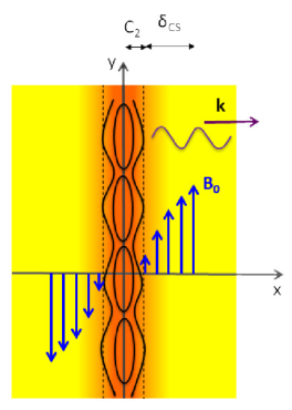
Figure 1: Schematic picture of generation of waves by the unstable reconnection region. Waves propagate outward from the reconnection region in plasma with density and magnetic field gradients (density decreases with distance from the center of the current sheet). $C_{2}$ is the half-width of the plasmoid-dominated current sheet, $\delta_{CS}$ is the density (magnetic field) gradient scale.

The simplifying assumptions in the analytical model are as follows: 1) For perturbations and background quantities only $\partial/\partial x\neq 0$. 2) We consider fast magnetoacoustic waves propagating in the direction normal to the current sheet, e.g. wave vector components are $k_{x}\neq 0;\,k_{y}=0$. This is a reasonable assumptions for waves with $k_{x}>>k_{y}$ generated by elongated plasmoids with high length to width ratio. Further, since waves with significant $k_{y}$ would be refracted back to the current sheet, we only consider those waves that otherwise could escape. 4) The amplitudes of waves are small so that MHD equations can be linearized. 5) In the linearization of the MHD equations, we assume that the velocity of the background flow (inflow to the reconnection site $V_{in}$) is zero. While in reconnection regions the velocity of the inflow is not zero, this approximation is reasonable since the inflow is expected to be significantly sub-Alfvenic $V_{in}\sim 0.01V_{A}$ (Huang & Bhattacharjee, 2010; Uzdensky et al., 2010) and fast mode waves propagate with the velocity $c_{f}=\sqrt{V_{A}^{2}+c_{s}^{2}}\sim V_{A}$ in a strongly magnetized plasma. Here $c_{s}$ is the sound speed in plasma. 6) Wave damping is neglected. 7) The background plasma is isothermal $T_{i}=T_{e}=T_{0}$. This implies that the sound speed is constant which simplifies the analytical treatment of the problem. Note that we will find a solution to the full wave equation without using the WKB approximation when a small wavelength is assumed. We will be considering waves of various wavelengths including those of the order of the half-thickness of the current sheet $\delta_{CS}$, where $\delta_{CS}$ is defined as the thickness of the region where plasma parameters change from their values in the current sheet to the values in the surrounding plasma undisturbed by reconnection (see Figure 1).

Table 1 presents a set of parameters of the coronal plasma for different plasma-$\beta$ and characteristic temporal and spatial scales used in our model. We choose the characteristic half-thickness of the current sheet to be $10^{4}$ km which is in the range of values inferred from observations $10^{3}-10^{5}$ km (Lin et al., 2015; Savage et al., 2010; Liu et al., 2010). To investigate wave reflection in current sheets in coronal plasma with different conditions we will vary plasma-$\beta$ in the range $0.02<\beta<1$.

Table 1: Characteristic parameters of plasma and magnetic field in the solar corona.

Parameter	Cool corona	Hot corona
Electron density $N_{0}$, $cm^{-3}$	$10^{9}$	$10^{9}$
Temperature $T_{0}$, K	$10^{6}$	$3\times 10^{6}$
Magnetic field $B_{0}$, G	10	10
Plasma-$\beta$ parameter $\beta=p_{th}/p_{mag}$	0.07	0.2
Alfvén speed $V_{A}$, km/s	690	690
Current sheet thickness $\delta_{CS}$, km	$10^{4}$	$10^{4}$
Characteristic timescale $\tau_{A}=\delta_{CS}/V_{A}$, s	14.5	14.5
Characteristic frequency $\nu^{*}$, $s^{-1}$	0.07	0.07

3 Frequencies of fast-mode waves

We consider the propagation of fast magnetoacoustic waves that are produced by the complex unstable magnetic reconnection process dominated by multiple plasmoids. Simulation results of Yang et al. (2015) support the idea that plasmoid ejections from the X-point generate fast waves propagating outward from the reconnection site. Thus it is reasonable to assume that frequencies and spatial scales of generated waves are related to those of the plasmoid dynamics in the reconnection current sheet. We will consider waves in the frequency range

$$\nu_{plsm}<\nu<<\nu_{i}$$ (1)

where $\nu_{plsm}$ is the minimal frequency of plasmoid ejection in the current sheet and $\nu_{i}$ is the ion-ion collision frequency in plasma. Wave frequencies have to be much smaller than the collision frequency since we describe the plasma as a fluid. For the solar coronal plasma with characteristic parameters in Table 1 the typical ion collision frequency is around $\nu_{i}\sim 2\,s^{-1}$. The frequency of plasmoid ejection can be estimated taking a ratio of the upstream Alfven speed and the characteristic length of the plasmoid $\nu_{plsm}=V_{A}/\lambda_{plsm}$.

It is reasonable to accept that a nonlinearly formed plasmoid is always longer than the thickness of the current sheet. Loureiro et al. (2012) presented resistive MHD simulations of reconnection at high Lundquist numbers up to $10^{7}$ showing formation of multiple elongated plasmoids with the length exceeding plasmoids width and much larger than the thickness of the current sheet between plasmoids. We assume a typical half-thickness of the current sheet to be $\delta_{CS}=10^{4}$ km and a plasmoid half-length that is few times larger $5\times 10^{4}$ km. Taking this estimate we obtain a range of frequencies and corresponding wave periods to consider;

$$0.01\,s^{-1}<\nu<<2\,{\rm s}^{-1}$$ (2)

$$0.5\,s<<T<2\,{\rm min}.$$ (3)

This frequency range is consistent with wave frequencies produced by plasmoid dynamics in previous MHD simulations. Yang et al. (2015) obtained frequencies of fast waves below $0.25\,s^{-1}$. Jelínek et al. (2017) reported wave period $\sim 25\,s$ generated by oscillating plasmoid. Below we will compare results for different parameters in dimensionless units therefore for the reference our frequency range in dimensionless units is $0.2<\hat{\nu}<<30$.

4 Analytical model

In this section we derive and solve the wave equation for fast mode waves propagating outward from the reconnection site in a non-uniform background plasma. In our analysis we will refer to the study of propagation of Alfvén waves in the atmosphere with the exponential profile of plasma density by Hollweg (1984). In the next subsection we briefly summarize this study.

4.1 Propagation of Alfvén waves in a non-uniform plasma

Hollweg (1984) considered a propagation of small-amplitude transverse (and non-compressive) Alfvén waves along an untwisted magnetic field $\mathbf{B}_{0}$ on a static background ($\mathbf{V}_{0}=0$). All quantities are axisymmetric relative to the vertical $z$-axis of asymmetry directed along $\mathbf{B}_{0}$ field implying that $\partial/\partial\theta=0$ where $\theta$ is the azimuthal angle.

Near the axis of asymmetry the wave equation for Alfvén waves has the form

$$\frac{\partial^{2}x}{\partial t^{2}}=V^{2}_{A}\frac{\partial^{2}x}{\partial s^{2}}.$$ (4)

Here $x\equiv\delta v_{\theta}/r$, $\delta v_{\theta}$ is the velocity disturbance and $s$ is the distance along the magnetic field line. When the Alfvén speed $V_{A}$ varies exponentially $V_{A}\varpropto e^{s/2h}$, then the equation has the following solution in terms of Hankel functions $H_{0}^{(1)}$ and $H_{0}^{(2)}$ of the first and second kinds, respectively,

$$x=[aH_{0}^{(1)}(\xi)+bH_{0}^{(2)}(\xi)]e^{i\omega t},$$ (5)

where $\xi\equiv 2h\omega/V_{A}(s)$, $\omega=2\pi\nu$, angular frequency, and $a$ and $b$ are complex constants. The corresponding magnetic field fluctuation can be derived from the linearized induction equation,

$$\delta\mathbf{B}_{\theta}=-\frac{ir\mathbf{B}_{0s}}{V_{A}}[aH_{1}^{(1)}(\xi)+bH_{0}^{(2)}(\xi)]e^{i\omega t}.$$ (6)

The time-averaged Poynting flux, $<\mathbf{S}>$, of the wave is

$$<\mathbf{S}>=-\mathbf{B}_{0}<\delta v_{\theta}\delta B_{\theta}>/4\pi.$$ (7)

With the solution for $\delta v_{\theta}$ and $\delta B_{\theta}$ given by (5) and (6) the Poynting flux along $\mathbf{B}_{0}$ is

$$<S_{s}>=\frac{B^{2}_{0s}r^{2}}{8\pi^{2}h\omega}\left(|a|^{2}-|b|^{2}\right).$$ (8)

From the form of Eq. (8), the parts of Eq. 5 associated with $H_{0}^{(1)}$ and $H_{0}^{(2)}$ are identified as the upward-propagating and downward-propagating waves, respectively.

Now consider a two-layer model in which $V_{A}$ varies exponentially for $s<0$ while $V_{A}=V_{Ac}=constant$ for $s>0$. $V_{A}$ and $B_{0s}$ are assumed to be continuous at $s=0$. Suppose that there is some unspecified source of waves in $s<0$. Above the source the solution will be given by equations (5) and (6) in $s<0$. But in $s>0$ the solution to equation (4) must be a pure plane wave

$$x=ce^{(i\omega t-iks)}$$ (9)

$$\delta\mathbf{B}_{\theta}=-\frac{k\mathbf{B}_{0s}}{\omega}\delta v_{\theta},$$ (10)

where $k=\omega/V_{Ac}$ is the wavenumber and c is now a complex constant. At $s=0$ the disturbances $\delta v_{\theta}$ and $\delta\mathbf{B}_{\theta}$ are continuous. These boundary conditiions allow to determine unknown complex constants. Then the wave energy reflection coefficient, R, i.e. the ratio of downgoing energy flux to upgoing energy flux in $s<0$ can be obtained as

$$R=\frac{|b|^{2}}{|a|^{2}}.$$ (11)

This completes the brief discussion of propagation and reflection of Alfvén waves in the non-uniform two-layer atmosphere presented in Hollweg (1984). In the following subsection we will carry out similar analysis for the fast mode waves propagating in plasma with varying density and magnetic field.

4.2 Propagation of fast waves in the neighborhood of a current sheet

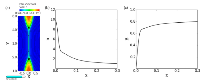
Figure 2: Resistive MHD simulation of reconnection in the isothermal Harris current sheet. a) colormap of plasma density $n$. Black arrows illustrate plasma velocity field. b) Density profile across the reconnection region at $x=0;\,y=3$. c) Magnitude of the reconnecting magnetic field across the reconnection region at $x=0;\,y=3$. This simulation is for plasma $\beta=0.07$ and resistivity $\eta=10^{-4}$ (or corresponding Lundquist number $S=10^{4}$).

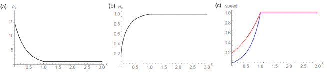
Figure 3: Typical profiles of plasma density (a) and reconnecting magnetic field component (b) used in the analytical model. Profiles of Afvén speed (blue curve) and fast magnetoacoustic speed (red curve) are shown on plot (c). Profiles were obtained assuming $\beta=0.07$ and $c_{0}=0.03$.

We choose to specify analytical profiles for the background plasma density and magnetic field in the vicinity of the reconnection region. Reconnection regions with strong plasma compressions are of particular interest since these are potential sources of hard energy spectra of particles accelerated by the Fermi process (Drury, 2012; Montag et al., 2017). In Provornikova et al. (2016) we performed resistive MHD simulations of Sweet-Parker-like laminar magnetic reconnection in different magnetic field geometries and with varying plasma parameters. In the highly conductive coronal plasma the Lundquist number $S\sim 10^{14}$ and reconnection current sheets are unstable to multiple plasmoid formation (Loureiro et al. 2012). In Provornikova et al. (2016) we limited our consideration to a single laminar reconnection region that , for the purposes of this paper, can represent the large scale reconnection region with the plasmoid substructure assumed to exist, and averaged over, within the macroscopic current sheet’s diffusion layer. Figure 2 shows an example of a simulated reconnection region with strong plasma compression, by a factor of 5. Panels b) and c) present the density and reconnecting field $B_{y}$ profiles across the reconnection region (due to the symmetry only $x>0$ is shown). We choose the analytical profiles that approximate profiles obtained in simulations. Let us assume that away from the reconnection region the undisturbed plasma is characterized by the plasma-$\beta$. The normalization parameters are the number density $N^{*}$, the Alfvén speed $V^{*}=V_{A}=B^{*}/\sqrt{N^{*}\mu_{0}}$, the magnetic field $B^{*}$, and the half-thickness of the current sheet $\delta_{CS}$ (Table 1). We approximate the density profile with the following piecewise function

$$n(x)=\left\{\begin{array}[]{ll}\left(\frac{1}{\beta}+1\right)e^{-\frac{C_{1}x+C_{2}}{x0}}&(0\leq x<1)\\ 1&(x\geq 1).\\ \end{array}\right.$$ (14)

Here $n(x)$ is the normalized number density and $x_{0}=\frac{1}{ln(1/\beta+1)}$. For the calculations we choose $C_{2}$ in the range $0<C_{2}<1$ and define $C_{1}$ as $C_{1}=1-C_{2}$. The constants are introduced to define the background plasma variations in the region outside of the plasmoid dominated current sheet with the half-width $C_{2}$ (see Figure 1). Hereafter parameters for region $0\leq x<1$ are denoted with the subscript 1 and for region $x\geq 1$ with subscript 2. We assume a constant magnetic field in region 2, $B(x)\equiv B_{2}=1$. To obtain a profile for the magnetic field in region 1 we use the condition of total pressure balance in the system which yields

$$B(x)=\left\{\begin{array}[]{ll}\sqrt{\left(1+\beta\right)\left(1-e^{-\frac{C_{1}x+C_{2}}{x0}}\right)}&(0\leq x<1)\\ 1&(x\geq 1).\\ \end{array}\right.$$ (17)

The profiles of plasma density and magnetic field given by (14) and (17) are shown in Figure 3 a) and b). The resulting Alfvén speed and fast magnetoacoustic speed profiles are shown in Figure 3 c).

We derive a solution of the wave equation for region 1. Following the standard procedure of linearization of a system of ideal MHD equations (Priest, 2014), accounting for the non-uniform background we obtain an equation for the velocity disturbance $\delta\mathbf{V^{\prime}}$

$$n_{0}\frac{\partial^{2}\delta\mathbf{V^{\prime}}}{\partial t^{2}}=\nabla\left(\left(\delta\mathbf{V^{\prime}}\cdot\nabla\right)p_{0}\right)+\nabla\left(c_{s}^{2}n_{0}\nabla\cdot\delta\mathbf{V^{\prime}}\right)+\frac{1}{\mu_{0}}\left[\nabla\times\left[\nabla\times\left(\delta\mathbf{V^{\prime}}\times\mathbf{B}_{0}\right)\right]\right]\times\mathbf{B}_{0}$$

$$+\frac{1}{\mu_{0}}\left(\nabla\times\mathbf{B}_{0}\right)\times\left[\nabla\times\left(\delta\mathbf{V^{\prime}}\times\mathbf{B}_{0}\right)\right],$$ (18)

where $n_{0}(x)$ and $\mathbf{B}_{0}(x)=(0,B_{0}(x),0)$ are the background number density and magnetic field given by Eqs. (14) and (17), respectively, $p_{0}$ is the plasma pressure, and $c_{s}$ is the (uniform) sound speed $c_{s}^{2}=2T=\beta/2$. We consider waves propagating along the $x$-axis perpendicular to $\mathbf{B}_{0}$ and we will look for a solution in a form $\delta\mathbf{V^{\prime}}=(\delta V(x)\exp(-i\omega t),0,0)$. Then equation (18) reduces to an equation for $\delta V(x)$

$$n_{0}(c_{s}^{2}+c_{A}^{2})\frac{d^{2}\delta V}{dx^{2}}+\frac{d\delta V}{dx}\left(\frac{dn_{0}(c_{s}^{2}+c_{A}^{2})}{dx}\right)+\delta Vn_{0}\omega^{2}=0$$ (19)

or

$$\frac{d}{dx}\left(n_{0}(c_{s}^{2}+c_{A}^{2})\frac{d\delta V}{dx}\right)=-\delta Vn_{0}\omega^{2}$$ (20)

where $c_{A}$ is the non-uniform Alfvén speed. Substituting for $B_{0}$ and $n_{0}$ with the expressions for region 1, Eqs. (17) and (14), we obtain

$$n_{0}(c_{s}^{2}+c_{A}^{2})=n_{0}\beta/2+B_{0}^{2}=1+\beta-\frac{1}{2}\left(1+\beta\right)e^{-\frac{C_{1}x+C_{2}}{x_{0}}}.$$ (21)

Equation (20) becomes

$$\frac{d}{dx}\left(\left(1+\beta-\frac{1}{2}\left(1+\beta\right)e^{-\frac{C_{1}x+C_{2}}{x_{0}}}\right)\frac{d\delta V}{dx}\right)=-\delta V\omega^{2}\left(\frac{1}{\beta}+1\right)e^{-\frac{C_{1}x+C_{2}}{x_{0}}}.$$ (22)

Introducing the variable $\xi(x)\equiv e^{-\frac{C_{1}x+C_{2}}{x_{0}}}-1$, equation (22) reduces to

$$\left(1-\xi^{2}\right)\frac{d^{2}\delta V(\xi)}{d\xi^{2}}-2\xi\frac{d\delta V(\xi)}{d\xi}+\frac{2x_{0}^{2}\omega^{2}}{\beta C_{1}^{2}}\delta V(\xi)=0.$$ (23)

The solution of this equation is a linear combination of the associated Legendre functions of first and second kind, $P_{p}(\xi)$ and $Q_{p}(\xi)$ (Abramowitz & Stegun, 1965, p. 332). The order $p$ of the functions is found by solving an equation $p(p+1)=\frac{2x_{0}^{2}\omega^{2}}{\beta C_{1}^{2}}$ and taking the positive root. The general solution of the equation (23) can be written in the following form,

$$\delta V(\xi)=c(P_{p}(\xi)-i\alpha Q_{p}(\xi))+d(P_{p}(\xi)+i\alpha Q_{p}(\xi)),$$ (24)

where the complex $c=c_{r}+ic_{i}$ and $d=d_{r}+id_{i}$ are coefficients to be found, and $\alpha$ is a coefficient defined at $\xi=0$ as $\alpha=\sqrt{-\frac{P_{p}(0)P_{p}^{\prime}(0)}{Q_{p}(0)Q_{p}^{\prime}(0)}}$ (see Appendix). Substituting $\xi(x)$ one can obtain the expression for $\delta V(x)$. The solution (24) multiplied by time dependence $e^{-i\omega t}$ represents the velocity disturbance $\delta V^{\prime}$ in a propagating fast-magnetoacoustic wave in the non-uniform region 1.

The time-averaged energy flux $<F>$ of fast magnetoacoustic waves can be calculated as a sum of the acoustic flux and Poynting flux and after normalization has the form

$$<F>=<\operatorname{Re}(\delta p^{\prime})\,\operatorname{Re}(\delta V^{\prime})+B_{0}\operatorname{Re}(\delta V^{\prime})\operatorname{Re}(\delta B^{\prime})>=$$ (25)

$$=<c_{s}^{2}\operatorname{Re}(\delta\rho^{\prime})\,\operatorname{Re}(\delta V^{\prime})+B_{0}\operatorname{Re}(\delta V^{\prime})\operatorname{Re}(\delta B^{\prime})>.$$

Here $\delta B^{\prime}=\delta B(x)e^{-iwt}$ and $\delta p^{\prime}=\delta p(x)e^{-iwt}=c_{s}^{2}\delta\rho(x)e^{-iwt}$ are the $y$-components of the magnetic field disturbance and plasma pressure disturbance, respectively. From the linearized induction equation $\frac{\partial\delta B^{\prime}}{\partial t}+\frac{\partial\left(\delta V^{\prime}B_{0}\right)}{\partial x}=0$ one can obtain $\delta B=-i/\omega(\partial(B_{0}\delta V)/\partial x)$. Similarly from the linearized continuity equation, $\delta\rho=-i/\omega(\partial(\rho_{0}\delta V)/\partial x)$. Thus using (24) we can derive an expression for the wave energy flux which has the form

$$<F>=\frac{1}{2\omega}\rho_{0}c_{f}^{2}\alpha(|c|^{2}-|d|^{2})(P_{p}^{\prime}Q_{p}-Q_{p}^{\prime}P_{p}).$$ (26)

The expression for the energy flux of fast mode waves is similar to the expression (8) derived by Hollweg (1984) and represents the difference in the energy flux of outgoing waves and reflected waves. From the form of Eq. (26) we identify the parts of Eq. (24) as outgoing and reflected waves, respectively,

$$\delta V_{out}=c(P_{p}-i\alpha Q_{p})e^{-i\omega t}$$ (27)

$$\delta V_{r}=d(P_{p}+i\alpha Q_{p})e^{-i\omega t}.$$ (28)

Now, similarly to Eq. (11) in the Hollweg study, we define the wave energy reflection coefficient as the ratio of fluxes of outgoing and reflected waves in Eq. (26),

$$R=\frac{|d|^{2}}{|c|^{2}}.$$ (29)

To calculate the reflection coefficient for various wave frequencies and plasma-$\beta$, it is required to determine complex constants $c$ and $d$.

In region 2, $x\geq 1$, where plasma parameters are constant the solution of the equation (18) is a plane wave,

$$\delta V_{t}=v_{t}e^{i(k_{t}x-\omega t)},$$ (30)

where $v_{t}$ is the amplitude of the wave, $k_{t}=\omega/c_{f}$ is the wave number, $c_{f}$ is the (constant) fast-mode speed in region 2. The subscript $t$ refers to the transmitted wave.

We have obtained a general solution for a fast magnetoacoustic wave propagating in the region 1 with non-uniform background density and magnetic field and a plane wave solution in uniform region 2. Since background $n_{0}$ and $B_{0}$, and therefore Alfvén speed $c_{A}$, are continuous at $x=1$ (see Figure 3), $\delta V$, $\delta\rho$ and $\delta B$ must also be continuous. Thus, assuming that at $x=0$ there is some source of waves with angular frequency $\omega$ and arbitrary small amplitude $V_{b}$, the boundary conditions are as follows,

$$\begin{array}[]{ll}x=0:&|\delta V_{out}|=V_{b}\,\,\text{and phase of}\,\,V_{out}\,\,\text{is zero}\\ x=1:&\delta V_{out}+\delta V_{r}=v_{t}e^{i(\omega/c_{f}+\phi)},\\ &\delta\rho_{out}+\delta\rho_{r}=\frac{\rho_{0}(1)}{c_{f}}v_{t}e^{i(\omega/c_{f}+\phi)}\\ &(\delta B_{out}+\delta B_{r})e^{\phi_{1}}=\frac{B_{0}(1)}{c_{f}}v_{t}e^{i(\omega/c_{f}+\phi)}.\end{array}$$ (35)

The conditions define the in-phase relation between $\delta V$, $\delta\rho$ and $\delta B$ in the transmitted wave since it is a fast wave propagating in the uniform plasma. The phase $\phi_{1}$ is introduced to ensure that $\delta B$ is continuous at $x=1$.

5 Reflection of fast mode waves

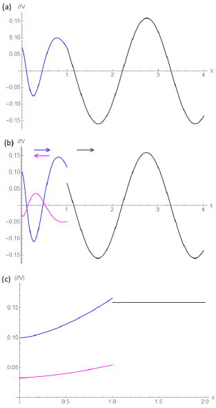
Figure 4: (a): Profile of $\delta V$ obtained from the solution of the wave equation. (b): Profiles of outgoing (blue curve), reflected (magenta) and transmitted (black) waves; (c) Profiles of amplitudes of outgoing (blue curve), reflected (magenta) and transmitted (black) waves.

Figure 4 shows a solution of wave equation (19) with boundary conditions (35), background plasma profiles shown in Figure 3 for the parameters $\beta=0.07$ and $C_{2}=0.01$, arbitrary wave amplitude $V_{b}=0.1$ at $x=0$ and wave angular frequency $\hat{\omega}=2\pi\hat{\nu}$ with $\hat{\nu}=0.5$. The plasma and magnetic field parameters for coronal plasma with $\beta=0.07$ are presented in Table 1. The corresponding wave frequency is $0.04$ $s^{-1}$. Figure 4 (a) shows the profile of $\delta V$ in a fast mode wave originating in the reconnection current sheet (at $x=0$) and propagating outward through the non-uniform plasma (blue curve in the region 1: $0<x<1$) and then in the uniform plasma (black curve in region 2: $x>1$) not disturbed by reconnection. Figure 4 (b) shows the decomposition of the wave into the outgoing from the reconnection current sheet (blue curve), reflected in region 1 due to gradients in plasma background (magenta) and transmitted into the uniform plasma (black). The profiles show the real parts of the complex expressions in Eqs. (27), (28) and (30). The outgoing and transmitted waves propagate along the positive direction of $x$-axis and the reflected wave propagates in the opposite direction towards the current sheet. The variations of the amplitudes of the three waves are shown in Figure 4 (c). In region 1 the amplitude of the outgoing wave increases as it propagates outwards due to the decreasing density with distance from the current sheet while the wave flux remains constant (the amplitude of the reflected wave decreases toward the reconnection current sheet for the same reason). The wavelength of the outgoing wave increases due to the increase of the Alfvén speed in region 1. In region 2 where background plasma parameters are constant, the solution is a plane wave with constant amplitude and wavelength. Wave reflection causes a difference between the amplitudes of the outgoing wave and the transmitted wave at $x=1$ (Figure 4 (c)).

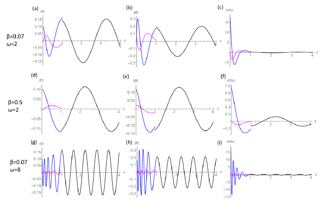
Figure 5: Profiles of velocity, density and magnetic field disturbances in outgoing (blue), reflected (magenta) and transmitted (black) fast magnetoacoustic waves for different plasma-$\beta$ and wave angular frequency: (a)-(c) $\beta=0.07$, $\hat{\omega}=2$; (d)-(f) $\beta=0.5$, $\hat{\omega}=2$; (g)-(i) $\beta=0.07$, $\hat{\omega}=8$.

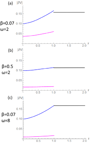
Figure 6: Amplitudes of outgoing (blue), reflected (magenta) and transmitted (black) waves for different cases; (a) $\beta=0.07$, $\hat{\omega}=2$; (b) $\beta=0.5$, $\hat{\omega}=2$; (c) $\beta=0.07$, $\hat{\omega}=8$.

To find conditions for efficient wave reflection of fast waves near the reconnection region we solve the wave equation for different plasma-$\beta$ and wave frequencies. Figure 5 presents the profiles of velocity, density and magnetic field disturbances in fast waves for plasma-$\beta$ parameters $\beta=0.07$ and $\beta=0.5$ and wave angular frequencies $\hat{\omega}=3$ and $\hat{\omega}=8$. Figure 6 shows the amplitude variations of $\delta V$ in outgoing, reflected and transmitted waves in the corresponding cases. In the lower-$\beta$ case, $\beta=0.07$, which is typical for coronal plasma, the amplitude of the reflected wave $|\delta V_{r}|$ is larger compared to the higher-$\beta$ case $\beta=0.5$ demonstrating stronger wave reflection near reconnection regions in lower-$\beta$ plasma. Also, comparison of cases (a) and (c) in Figure 6 with same $\beta=0.07$ but different wave angular frequencies $\hat{\omega}=2$ and $\hat{\omega}=8$ shows that the amplitude of the reflected wave is larger for lower-frequency waves. This suggests that the lower frequency waves produced in reconnection are reflected more efficiently than higher frequency waves. In the higher frequency case (Figure 6 c)) the amplitude of the transmitted wave almost matches the amplitude of the outgoing wave at $x=1$, meaning that the outgoing fast wave propagates away from the reconnection region almost without reflection.

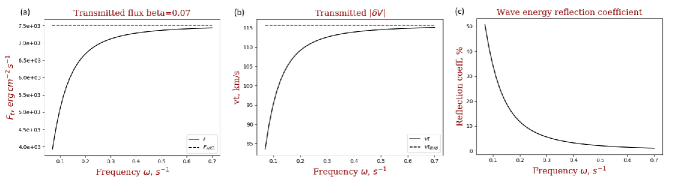
Figure 7: (a) Transmitted wave energy flux $F_{t}$ as a function of wave angular frequency in a range $0.07\,s^{-1}<\omega<0.7\,s^{-1}$ and comparison with WKB flux. For all frequencies $|\delta V|_{x=0}=0.1$. (b) Amplitude of velocity disturbance in transmitted fast magnetoacoustic wave $v_{t}$ and comparison with WKB value; (c) Dependence of wave energy reflection coefficient on wave angular frequency.

Figure 7 a) shows the transmitted wave energy flux $F_{t}$ calculated as a sum of Poynting and acoustic fluxes according to (26) as a function of wave angular frequency in a range $0.07\,s^{-1}<\omega<0.7\,s^{-1}$ for plasma beta $\beta=0.07$ and the comparison with the wave flux in WKB approximation. If the WKB approximation were valid, no reflection would occur and we would obtain the value of the flux $F_{WKB}=\rho_{0}(0)V_{b}^{2}c_{f}(0)/2$ equal to the flux of outgoing waves at $x=0$ independent of the frequency. This value is indicated by the horizontal dashed line marked WKB. The calculated values of transmitted flux are lower than the WKB value because of the wave reflection near the reconnection current sheet. The difference is more noticeable for lower frequencies when wave reflection is more efficient. The transmitted flux approaches the WKB value at high frequencies as the WKB approximation becomes valid. Figure 7 b) shows the amplitude of the velocity disturbance in the transmitted wave $v_{t}$ as a function of frequency. If the WKB approximation were valid we would obtain the value $v_{t,WKB}=\sqrt{2F_{WKB}/(c_{f,II}\rho_{0,II})}$ assuming that the wave flux $F_{WKB}$ is constant in this limit. The WKB amplitude $v_{t}$ is shown by the dashed horizontal line. Again, wave reflection causes lower amplitude $v_{t}$ compared to the WKB value; this effect is more noticable at lower frequencies. Figure 7 c) similarly shows the wave energy reflection coefficient as a function of angular frequency as calculated according to Eq. (29). For lower wave frequencies $\nu\sim 0.01\,s^{-1}$, a significant fraction of wave energy can be reflected, up to 50 %. The wave energy reflection coefficient drops quickly with increasing wave frequency. Higher frequency waves propagate to the surrounding plasma almost without reflection.

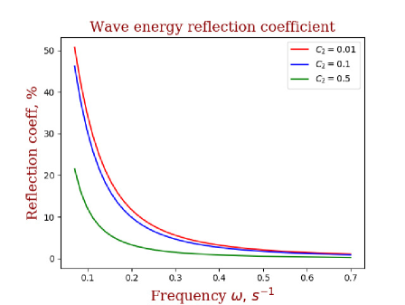
Figure 8: Dependence of wave energy reflection coefficient on wave angular frequency for different values of $C_{2}$. Plasma-$\beta$ parameter is $\beta=0.07$.

We have also calculated wave energy reflection coefficients for different values of half-width of plasmoid-dominated current sheet $C_{2}$ (see Figure 8). For the same background plasma parameters, greater $C_{2}$ values correspond to reconnection sites with more turbulent current sheets, where the laminar region of applicability of our analytical model is reduced. In such reconnection sites, for a given wave frequency, a smaller fraction of wave energy is reflected back towards the current sheet. However, one might also anticipate a broader range of wave frequencies and a higher intensity of wave generation within more turbulent reconnection current sheets.

The wave energy reflection coefficient $R$ as a function of wave angular frequency in the range $0.07\,s^{-1}<\omega<0.7\,s^{-1}$ calculated for different plasma-beta’s $\beta=0.02,\,0.07,\,0.2,\,0.5$ is shown in Figure 9. The reflection coefficient is greater for waves of lower frequencies near reconnection regions in strongly magnetized plasma with $\beta<<1$. For example, up to 40 % of the energy carried by waves with frequencies 0.01 $s^{-1}$ will be reflected near the reconnection region in plasma with $\beta=0.07$ and even stronger reflection, up to 60 %, is expected for $\beta=0.02$.

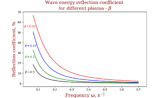
Figure 9: Wave energy reflection coefficient for different plasma-$\beta$ for a range of wave angular frequencies

6 Role of wave reflection for particle acceleration in reconnection

In resistive MHD simulations in Provornikova et al. (2016), we showed that strong plasma density compressions can form in reconnection current sheets with a guide field $B_{g}=0$ in low-$\beta$ plasma. The compression is higher when the background plasma-$\beta$ is smaller, due to the extra thermal pressure required for pressure balance with the external magnetic field. The presence of a guide field reduces the compression, as expected. Recent kinetic simulations by Li et al. (2018) of plasmoid reconnection in low-$\beta$ plasma also show regions of high plasma compression, although compressions appear in contracting islands rather than in current sheets. In analysis of type III radio bursts Chen et al. (2018) reconstructed the trajectories of electron beams in a flare and showed the presence of steep density gradients (5-29 Mm scale length as an upper limit) near the flare site (see also Chen et al. (2013)). These observations support the conclusion that reconnection regions with high compressions exist in the corona. Results in this paper suggest that waves generated within magnetic reconnection sites with high degree of plasma compression can undergo internal reflections due to the strong Alfvén speed gradients near the reconnection region. In a lower-$\beta$ plasma the reflection becomes more efficient. In our analytical treatment we assumed the guide field component to be zero. The effect of the guide field would reduce the Alfvén speed gradient near the reconnection region and therefore the wave reflection.

Strong plasma compression and efficient wave reflection in reconnection regions in low-$\beta$ plasma provide appropriate conditions for Fermi particle acceleration across the current sheet with resulting hard energy spectra. Drury (2012) showed that with a higher compression ratio a harder particle energy spectrum forms (low $\gamma<5$ in a particle distribution function $f(v)\sim v^{-\gamma}$). In this process particles bounce between the incoming reconnecting flows scattered by waves. The presence of waves around the reconnection region is critical for this mechanism to work so that particles bounce multiple times across the current sheet and gain more energy. Waves produced by reconnection and their reflection facilitate efficient particle scattering. Further research is needed to explore the formation of power-law distributions and confirm the relation between the spectral index and compression ratio (Drury, 2012) in such reconnection regions, in particular of ions, since electrons, with much smaller gyroradii, do not participate effectively in first order Fermi acceleration across the current sheet. Instead, electrons can be energized by a first order Fermi acceleration process while reflecting back and forth within in the contracting plasmoids (Drake et al. 2006).

The analytical conclusion that reconnection regions with strong compression are a source for hard power-law ion distribution (Drury, 2012) is supported by the analysis of Fermi acceleration of electrons in plasmoids with the incorporation of compressibility effects by Montag et al. (2017). They generalized the incompressible theory of electron acceleration in contracting plasmoids by Drake et al. (2013) and derived analytically the dependence of spectral index $\gamma$ of electron distribution on the compressibility $\partial n/\partial t$. Compressional effects cause a decrease of the $\gamma$ value implying that Fermi acceleration in the presence of compressions produces harder power-law spectra (see also Li et al., 2018; le Roux et al., 2015). They also found that a guide field of the order of the reconnecting field effectively suppresses the development of a power-law distribution.

Magnetic nulls in the solar corona are thought to be key structures for magnetic reconnection to occur. The nulls are associated with strong gradients of magnetic field, and additionally high plasma compression can form (Provornikova et al., 2016) producing gradients of Alfvén speed. With these properties magnetic nulls represent regions where magnetic reconnection can effectively produce hard power-law distributions of particles accelerated by first Fermi mechanism in plasmoids (electrons) and current sheets (ions).

7 Role of reconnection generated waves for the FIP effect

Alfvén and fast mode waves are a key agent in the chromospheric fractionation of plasma to produce the First Ionization Potential (FIP) Effect. Pottasch (1963) first suggested that the elemental composition of the solar corona might be different to that of the underlying photosphere. Elements with FIP below about 10 eV, i.e. those like Fe, Si, and Mg, which are predominantly ionized in the chromosphere, are seen to be enhanced in abundance in the corona by a factor of about three. High FIP elements (e.g. H, O, Ar) remain unchanged, though the highest FIP elements (He, Ne) may be still further depleted. A compelling explanation for this abundance anomaly has emerged (Laming, 2015) whereby the ponderomotive force due to Alfvén (or fast mode) waves propagating through or reflecting from the chromosphere acts on chromospheric ions and in solar conditions, giving them an extra acceleration upwards into the corona.

The most successful models of the abundance anomaly, including the extra depletion of He and Ne, appear to arise when the Alfvén wave travel time between one loop footpoint and the other is an integral number of Alfvén wave half periods, i.e. when the loop is in resonance with the waves. Since the FIP effect is widely observed in the solar corona, on different sized loops with presumably different magnetic fields, the most plausible scenario for the wave origin would be coronal (Rakowski & Laming, 2012; Laming, 2017), presumably reconnection, in which waves resonant with the coronal loop would be a natural consequence.

In stars of later spectral type than the Sun, the FIP effect decreases, and eventually inverts for M dwarfs (e.g. Wood & Laming, 2013). An “Inverse FIP Effect” has also been observed in a solar flare plasma above a sunspot (Doschek et al., 2015). In these cases the coronal Alfvén waves propagating down to the chromosphere before reflecting back up into the corona must give way to a population of similar waves coming up from below before reflecting back down again. We argue that the decrease in the coronal wave amplitude at later spectral type, which effectively means higher magnetic field, is most likely due to the effects discussed in this paper, i.e. in higher ambient magnetic fields (lower plasma-$\beta$), fewer waves emitted from the reconnection current sheet can escape to infinity to cause FIP fractionation. More are trapped locally, resulting in increased plasma heating and particle acceleration.

8 Conclusions

Due to the highly unsteady, structured and impulsive nature of magnetic reconnection, it is natural to expect the generation of MHD waves of different modes when reconnection occurs in the solar corona. Several observations of waves and oscillations associated with flares suggest their origin in magnetic reconnection. Waves produced in reconnection potentially play an important role in particle energization and elemental fractionation. In particular, the presence of waves in reconnecting inflows is critical for the development of magnetic turbulence scattering particles across current sheets in the first order Fermi acceleration, and the presence of waves far from the current sheet can give rise to a ponderomotive force to provide ion-neutral FIP fractionation. In this work we aimed to explore how fast magnetoacoustic waves, presumably generated by reconnection, propagate outward from the reconnection site and what fraction of the wave energy flux is reflected and transmitted to the surrounding plasma.

We obtained an analytical solution that describes the propagation of fast waves in non-uniform plasma near the reconnection region. Due to the Alfvén speed gradient, fast waves produced by unsteady reconnection can undergo reflection within the reconnection site. Wave reflection is most efficient near the reconnection current sheets in strongly magnetized plasma ($\beta<<1$) and for waves with lower frequencies. We have calculated the wave energy reflection coefficient for various plasma-$\beta$ and a range of wave frequencies. For example, for lower frequency waves, in our calculations $\nu\sim 0.01\,s^{-1}$, and plasma with $\beta=0.07$, which is characteristic of the quiet solar corona, about 40 % of wave energy flux is reflected back toward the reconnection region. The fraction increases up to 60 % in a lower-$\beta$ plasma $\beta=0.02$ characteristic of the coronal active regions. For waves with higher frequencies, around $1\,s^{-1}$, the reflection coefficient drops to 2 %.

We considered waves propagating perpendicular to the current sheet with zero k-component along the B-field. While this assumption is valid for waves with $k_{x}>>k_{y}$ (in 2D picture) generated by elongated plasmoids, waves with various k-vector components will be produced by the highly irregular process of plasmoid formation and propagation. The effect of wave reflection will still be present with the reflection coefficient additionally depending on the direction of wave propagation. The propagation and reflection of waves near two- and three-dimensional plasmoid-dominated reconnection is a subject of the future work that will combine analytical and numerical approaches.

In the solar corona magnetic null points are topological structures considered as locations where magnetic reconnection is most probably to occur. Results presented in this paper and our previous study (Provornikova et al., 2016) suggest that reconnection at the nulls could also supply solar corona with suprathermal particles with hard energy spectra. Determining the acceleration mechanisms and magnetic structures where hard energy spectra of particles can be produced will help to understand the origin of suprathermal “seed” particles in the corona. The suprathermal population is required for production of solar energetic particles (SEP) in the corona. Laming et al. (2013) have argued that a hard energy spectrum of suprathermal “seed” particles is necessary for the injection into the acceleration at CME shocks with low Mach number within a few solar radii from the Sun. They suggested that these particles can originate in continuous reconnection processes in the corona. We will further investigate the efficiency of the first-order Fermi acceleration in current sheets for ion energization, in particular in reconnection regions with multiple plasmoids and small scale current sheets, and .

We also considered implications of wave reflection for element fractionation in stellar coronae. In active strongly magnetized coronae of later spectral type stars, waves produced in magnetic reconnection would be trapped locally meaning that less waves propagate from reconnection sites to infinity. Consequently, these effects cause a diminishing of the chromospheric ponderomotive force that provides extra acceleration to ions from the photosphere to the corona and generates FIP fractionation in stellar coronae. We suggest that the efficient wave reflection in reconnection processes in strongly magnetized stellar atmospheres could be a possible explanation of the diminished FIP fractionation observed in later spectral type.

Appendix A Appendix

The solution of equation (23) for the coordinate dependent part $\delta V(x)$ of the velocity disturbance $\delta{V^{\prime}}(x,t)=\delta V(x)\exp(-i\omega t)$ is a linear combination of the associated Legendre functions of first and second kind $P_{p}(x)$ and $Q_{p}(x)$. We will look for a linear combination that represents a sum of counter propagating waves, outgoing and reflected, which has a form

$$\delta V(x)=c(P_{p}(x)-i\alpha Q_{p}(x))+d(P_{p}(x)+i\alpha Q_{p}(x))$$ (A1)

For an arbitrary value of $\alpha$, the amplitudes of these two waves, $A_{out}(x)=|c|\sqrt{P_{p}^{2}+\alpha^{2}Q_{p}^{2}}$ and $A_{r}(x)=|d|\sqrt{P_{p}^{2}+\alpha^{2}Q_{p}^{2}}$ respectively, are oscillating functions of $x$ (see Fig 10 (a)). That means that with arbitrary $\alpha$ each of the two waves contains an outgoing and a reflected component. However a value of $\alpha$ exists when $A(x)=\sqrt{P_{p}^{2}+\alpha^{2}Q_{p}^{2}}$ is a monotonically increasing function of $x$, e.g. for this $\alpha$, $A^{\prime}(x)\geq 0$. In this case the combinations $c(P_{p}(x)-i\alpha Q_{p}(x))$ and $d(P_{p}(x)+i\alpha Q_{p}(x))$ define purely outgoing and reflected waves, respectively. To find $\alpha$ we solve inequality $A^{\prime}(x)=P_{p}P^{\prime}_{p}+\alpha^{2}Q_{p}Q^{\prime}_{p}\geq 0$. When $Q_{p}Q^{\prime}_{p}=0$ the product $P_{p}P^{\prime}_{p}$ also equals 0 (see Fig 10 (b)) so the inequality holds. At all intervals where $Q_{p}Q^{\prime}_{p}>0$ (Fig 10 (b)) the condition for the $\alpha$ parameter is $\alpha^{2}\geq-\frac{P_{p}(x)P^{\prime}_{p}(x)}{Q_{p}(x)Q^{\prime}_{p}(x)}$. The function $-\frac{P_{p}(x)P^{\prime}_{p}(x)}{Q_{p}(x)Q^{\prime}_{p}(x)}$ is shown in Fig 10 (c). For intervals where $Q_{p}Q^{\prime}_{p}<0$ (Fig 1A (b)) the condition for $\alpha$ is $\alpha^{2}\leq-\frac{P_{p}(x)P^{\prime}_{p}(x)}{Q_{p}(x)Q^{\prime}_{p}(x)}$. The only value of $\alpha$ that satisfies the two conditions at all intervals is $\alpha=\sqrt{-\frac{P_{p}(0)P^{\prime}_{p}(0)}{Q_{p}(0)Q^{\prime}_{p}(0)}}$. Figure 10 (c) shows the value of $\alpha^{2}=-\frac{P_{p}(0)P^{\prime}_{p}(0)}{Q_{p}(0)Q^{\prime}_{p}(0)}$ by the red dashed line. With this choice of the $\alpha$ parameter, the amplitudes of the outgoing and reflected waves are monotonically increasing functions as shown in Figures 4 c) and 6.

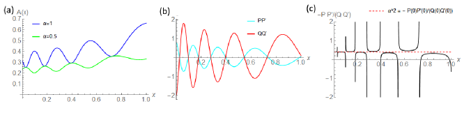
Figure 10: (a) Amplitude $A(x)=\sqrt{P_{p}^{2}+\alpha^{2}Q_{p}^{2}}$ as a function of $x$ for the order $p=9.4$ of Legendre functions and two arbitrary values of $\alpha=0.5;\,1$. (b) $P_{p}(x)P^{\prime}_{p}(x)$ and $Q_{p}(x)Q^{\prime}_{p}(x)$ as functions of $x$ for the order $p=9.4$. (c) Black curve: function $-\frac{P_{p}(x)P^{\prime}_{p}(x)}{Q_{p}(x)Q^{\prime}_{p}(x)}$ for the order $p=9.4$. Red dashed line: the constant $\alpha^{2}=-\frac{P(0)P(0)^{\prime}}{Q(0)Q(0)^{\prime}}$.

References

- Abramowitz & Stegun (1965) Abramowitz, M., Stegun, I. A. 1965, Dover Publications, INC., New York
- Brannon et al. (2015) Brannon, S. R., Longcope, D. W., Qiu, J. 2015, ApJ, 810, 4
- Chen et al. (2018) Chen, B. et al. 2018 (in preparation)
- Chen et al. (2013) Chen, B., Bastian, T. S., White, S. M., Gary, D. E. et al. 2013, ApJ, 763, L21
- Doschek et al. (2015) Doschek, G. A., Warren, H. P., & Feldman, U. 2015, ApJ, 808, L7
- Drake et al. (2006) Drake, J. F., Swisdak, M., Che, H., & Shay, M. A. 2006, Nature, 443, 553
- Drake et al. (2013) Drake, J. F., Swisdak, M., Fermo, R. 2013, ApJ, 763, L5
- Drury (2012) Drury, L. O. 2012, MNRAS, 422, 2474
- Fletcher & Hudson (2008) Fletcher, L., Hudson, H. S. 2008, ApJ, 675, 1645
- Huang & Bhattacharjee (2010) Huang, Y.-M., & Bhattacharjee, A. 2010, Physics of Plasmas, 17, 062104
- Hollweg (1984) Hollweg, J. V. 1984, ApJ, 277, 392
- Jelínek et al. (2017) Jelínek, P., Karlický, M., Van Doorsselaere, T., Bárta, M. 2017, ApJ, 847, 98
- Kigure et al. (2010) Kigure, H., Takahashi, K., Shibata, K., Yokoyama, T., & Nozawa, S. 2010, PASJ, 62, 993
- Krymskii (1977) Krymskii, G. F. 1977, Akademiia Nauk SSSR Doklady, 234, 1306
- Laming et al. (2013) Laming, J. M., Moses, J. D., Ko, Y.-K., et al. 2013, ApJ, 770, 73
- Laming (2015) Laming, J. M., 2015, Living Reviews in Solar Physics, 12, 2
- Laming (2017) Laming, J. M., 2017, ApJ, 844, 153
- Lee et al. (2014) Lee, E., Lukin, V. S., & Linton, M. G. 2014, A&A, 569, A94
- le Roux et al. (2015) le Roux, J. A., Webb, G. M., Zank, G. P., & Khabarova, O. 2015, Journal of Physics Conference Series, 642, 012015
- Li et al. (2018) Li, X., Guo, F., Li, H., & Birn, J. 2018, arXiv:1801.02255
- Lin et al. (2015) Lin, J., Murphy, N., Shen, C., Raymond, J. et al. 2015, Space Sci. Rev., 194, 237
- Liu et al. (2011) Liu, W., Title, A., Zhao, J., Ofman, L. et al. 2011, ApJ, 736, L13
- Liu et al. (2010) Liu, R., Lee, J., Wang, T., et al. 2010, ApJ, 723, L28
- Loureiro et al. (2005) Loureiro, N. F., Cowley, S. C., Dorland, W. D., Haines, M. G., & Schekochihin, A. A. 2005, Physical Review Letters, 95, 235003
- Loureiro et al. (2007) Loureiro, N. F., Schekochihin, A. A., & Cowley, S. C. 2007, Physics of Plasmas, 14, 100703
- Loureiro et al. (2012) Loureiro, N. F., Samtaney, R., Schekochihin, A. A., & Uzdensky, D. A. 2012, Physics of Plasmas, 19, 042303
- Melrose (1986) Melrose, D.B. 1986, Instabilities in Space and Laboratory Plasmas (Cambridge: Cambridge Univ. Press)
- McLaughlin & Hood (2004) McLaughlin, J. A., & Hood, A. W. 2004, A&A, 420, 1129
- McLaughlin & Hood (2006) McLaughlin, J. A., & Hood, A. W. 2006, A&A, 452, 603
- McLaughlin et al. (2009) McLaughlin, J. A., De Moortel, I., Hood, A. W., & Brady, C. S. 2009, A&A, 493, 227
- McLaughlin et al. (2017) McLaughlin, J. A., Nakariakov, V. M., Dominique, M., Jelínek, P., Takasao, S. in press?
- Montag et al. (2017) Montag, P., Egedal, J., Lichko, E., Wetherton, B. 2017, Physics of Plasma, 24, 062906
- Pottasch (1963) Pottasch, S. R. 1963, ApJ, 137, 945
- Priest (2014) Priest, E. 2014, Magnetohydrodynamics of the Sun, by Eric Priest, Cambridge, UK: Cambridge University Press, 2014,
- Provornikova et al. (2016) Provornikova, E., Laming, J. M., Lukin, V. S. 2016, ApJ, 825, 55
- Rakowski & Laming (2012) Rakowski, C. E., & Laming, J. M., 2012, ApJ, 754, 65
- Reep et al. (2016) Reep, J. W., Russel, A. J. B. 2016, ApJ, 818, L20
- Savage et al. (2010) Savage, S. L., McKenzie, D. E., Reeves, K. K. et al. 2010, ApJ, 722, 329
- Shen & Liu (2012) Shen, Y., Liu, Y. 2012, ApJ, 753, 53
- Tarr et al. (2017) Tarr, L. A., Linton, M., & Leake, J. 2017, ApJ, 837, 94
- Uzdensky et al. (2010) Uzdensky, D. A., Loureiro, N. F., & Schekochihin, A. A. 2010, Physical Review Letters, 105, 235002
- Wood & Laming (2013) Wood, B. E., & Laming, J. M. 2013, ApJ, 768, 122
- Wyper & Pontin (2014) Wyper, P. F., & Pontin, D. I. 2014, Physics of Plasmas, 21, 082114
- Yang et al. (2015) Yang, L., Zhang, L., He, J., Peter, H. et al. 2015, ApJ, 800, 111