Semileptonic decay of $B^{-}_{c}$ into $X(3930)$, $X(3940)$, $X(4160)$

Abstract

We study the semileptonic decay of $B^{-}_{c}$ meson into $\bar{\nu}l^{-}$ and the isospin zero $X(3930)~{}(2^{++})$, $X(3940)~{}(0^{++})$, $X(4160)~{}(2^{++})$ resonances. We look at the reaction from the perspective that these resonaces appear as dynamically generated from the vector-vector interaction in the charm sector, and couple strongly to $D^{*}\bar{D^{*}}$ and $D^{*}_{s}\bar{D_{s}^{*}}$. We also look into the $B^{-}_{c}\rightarrow\bar{\nu}_{l}l^{-}D^{*}\bar{D^{*}}$ and $B^{-}_{c}\rightarrow\bar{\nu}_{l}l^{-}D^{*}_{s}\bar{D_{s}^{*}}$ reactions close to threshold and relate the $D^{*}\bar{D^{*}}$ and $D^{*}_{s}\bar{D_{s}^{*}}$ mass distribution to the rate of production of the $X$ resonances.

I Introduction

The $X,Y,Z$ states, that challenge the constituent quark model picture of meson Godfrey:1985xj ; Vijande:2004he have been one of the most spectacular findings in hadron spectroscopy recently Chen:2016qju ; Liu:2013waa ; Godfrey:2008nc ; Guo:2017jvc . Their advent has stimulated much theoretical work aimed at unravelling their structure. Tetraquark pictures have been proposed Chen:2016oma ; Esposito:2016noz as well as molecular pictures stemming from the interaction of more elementary mesons Ortega:2012rs ; Molina:2009ct ; Guo:2017jvc . One of these pictures deals with the interaction of vector mesons with charm, leading to hidden charm quasibound meson states Molina:2009ct . In that work, the channels $D^{*}\bar{D^{*}}$, $D^{*}_{s}\bar{D_{s}^{*}}$, $K^{*}\bar{K}^{*}$, $\rho\rho$, $\omega\omega$, $\phi\phi$, $J/\psi J/\psi$, $\omega J/\psi$, $\phi J/\psi$, $\omega\phi$ were considered and the interaction between them was obtained using an extention of the local hidden gauge approach Bando:1987br ; Harada:2003jx ; Meissner:1987ge , exchanging vector mesons, and through contact terms provided by the theory. Some quasibound states were found which could be associated to known resonances. These states were: one state around $3943$ MeV with $I^{G}[J^{PC}]=0^{+}[0^{++}]$, which was associated to the $X(3940)$ Abe:2004zs ; Abe:2007jna ; another state around 3922 MeV with $0^{+}[2^{++}]$, which was associated to the $X(3930)$ Uehara:2005qd (now classified in the PDG Patrignani:2016xqp as the the $\chi_{c2}(2P)$ ), which could also correspond to the $X(3915)$ Zhou:2015uva ; Ortega:2017qmg , and a third one at $4169$ MeV with $0^{+}[2^{++}]$ that was associated to the $X(4160)$ Abe:2007sya .

The $X(3940)$ was found to couple mostly to $D^{*}\bar{D^{*}}$ in  Molina:2009ct , the $X(3930)$ also had its strongest coupling to $D^{*}\bar{D^{*}}$ and the $X(4160)$ had its strongest coupling to $D^{*}_{s}\bar{D_{s}^{*}}$. The light vector-vector channels couple weakly to those states, but given the large space available, they are the biggest source of the width, which in the theoretical work is also found in reasonable agreement with experiment. It is interesting to mention that there is a large list of works suggesting a bound $D^{*}_{s}\bar{D_{s}^{*}}$ state Liu:2009ei ; Branz:2009yt ; Weinberg:1965zz ; Baru:2003qq ; Chen:2015fdn ; Karliner:2016ith . QCD sum rules, although with its usual large uncertainties, have also speculated on this possibility Albuquerque:2009ak ; Zhang:2009st . The curious thing is that all these work aimed at reproducing the $X(4140)$ resonance not the $X(4160)$. One can think that the fact that light vector channels were not included as coupled channel in these studies had as a consequence a small width for the resonance which made it more appealing to have it associated to the $X(4140)$. Yet, the quantum numbers $0^{+}[1^{++}]$ for this resonance determined lately make the association of the state found in these works to the $X(4140)$ inappropriate, while the association to the $X(4160)$ is more natural.

The discussion on these states becomes more actual when one recalls the experimental work Aaij:2016iza ; Aaij:2016nsc in the $B^{+}\to J/\psi\phi K^{+}$ reaction, where the data analysis brought the surprising result that the $X(4140)$ has a width of around $\Gamma\simeq 83$ MeV, while former experiments give a width around $19$ MeV Aaltonen:2009tz ; Brodzicka:2010zz ; Aaltonen:2011at ; Aaij:2012pz ; Chatrchyan:2013dma ; Abazov:2013xda ; Lees:2014lra ; Abazov:2015sxa . This puzzle found a reasonable explanation in a recent work Wang:2017mrt , where the $J/\psi\phi$ invariant mass distribution at low invariant masses was analyzed in terms of the $X(4140)$ and $X(4160)$ and the mass distribution was better reproduced.

The result of this new analysis was that the $X(4140)$ has a width compatible with $19$ MeV, and it is the $X(4160)$ resonance the one that fills the strength in that region. The striking thing is that, since the $X(4160)$ in that work is supposed to be a $D^{*}_{s}\bar{D_{s}^{*}}$ bound state, but with a relatively large coupling to $J/\psi\phi$ in the coupled channels study of Molina:2009ct , when the $J/\psi\phi$ mass distribution is studied, a large cusp structure develops in this distributions at the $D^{*}_{s}\bar{D_{s}^{*}}$ threshold and such cusp is present in the experiment.

In view of this puzzling situation, any other reaction that brings light into these issues should be most welcome. This is the purpose of the present work, where we propose to measure the semileptonic decay of $B^{-}_{c}\rightarrow\bar{\nu}_{l}l^{-}X_{i}$, with $X_{i}$ any of the three resonances, $X(3930)$, $X(3940)$, $X(4160)$. Actually, this reaction has been studied recently wangzang from the perspective that the $X(3940)$ and $X(4160)$ resonances are radial high excitations of the charmonium states, corresponding to the $\eta_{c}(3S)$ and $\eta_{c}(4S)$ respectively. Our picture, where these resonances are generated from the interaction of vector meson with charm is quite different and the study of the $B_{c}\rightarrow\nu_{e}e^{+}X_{i}$ decays from this perspective is worth pursuing.

The use of semileptonic weak decays aiming at determining the structure of resonances has been exploited before in different cases. In Navarra:2015iea the $B_{s}$ and $B$ semileptonic decays, $\bar{B}^{0}_{s}\rightarrow D^{*}_{s0}(2317)\bar{\nu}_{l}l^{-}$, $\bar{B}^{0}\rightarrow D^{*}_{0}(2400)^{+}\bar{\nu}_{l}l^{-}$ were studied and compared to related reactions like $\bar{B}^{0}_{s}\rightarrow(DK)^{+}\bar{\nu}_{l}l^{-}$. In Sekihara:2015iha the production of light scalar mesons and light vector mesons was also investigated in semileptonic decays of $D$ and $D_{s}$ mesons. In Ikeno:2015xea the $\Lambda_{c}\rightarrow\Lambda(1405)e^{+}\nu_{e}$ was studied, looking at the decays of $\Lambda(1405)$ into $\pi^{+}\Sigma^{-}$, $\pi^{-}\Sigma^{+}$, $\pi^{0}\Sigma^{0}$ and $\bar{K}N$ production. In this case the weak decay filters $I=0$ in the final meson baryon system, which makes this reaction special to investigate the properties of the $\Lambda(1405)$. Related to these works, but with a different aim, one has the work of Liang:2016exm where the $\Lambda_{b}\rightarrow\Lambda_{c}(2595)\bar{\nu}_{l}l$ and $\Lambda_{b}\rightarrow\Lambda_{c}(2625)\bar{\nu}_{l}l$ decays are studied in order to test the pseudoscalar-baryon and vector-baryon components of the $\Lambda_{c}(2595)$ and $\Lambda_{c}(2625)$ resonances Liang:2014kra .

In the present work we take advantage of these previous studies and calculate the $B_{c}\rightarrow\nu_{l}l^{+}X_{i}$ decay rates and compare them with the $B_{c}\rightarrow\nu_{l}l^{+}D^{*}\bar{D^{*}}$, $\nu_{l}l^{+}D^{*}_{s}\bar{D_{s}^{*}}$ decays. We establish a link between these processes which is tied to the molecular nature of these resonances, making predictions to be tested in future experiments from where much valuable information concerning the nature of these states is to be expected.

II Formalism

The $B^{-}_{c}\rightarrow\bar{\nu}e^{-}X$ process proceeds at the quark level through a first step shown in Fig. 1. The process involves the $bc$ weak transition, which is the same one as in the $B$ decays studied in Ref. Navarra:2015iea .

There is, however, a novelty in the present process. Indeed, if we want to see two mesons, the $c\bar{c}$ quarks of Fig. 1 must hadronize into two mesons components. This is easily done for mesons since one introduces an extra $\bar{q}q$ pair with vacuum quantum number, $\bar{u}u+\bar{d}d+\bar{s}s+\bar{c}c$, and then the two quarks after the weak process participate in the formation of the two mesons. With two quarks after the weak vertex, as in Fig. 2, the new $\bar{q}q$ pair can be placed in between these $c\bar{c}$ quarks.

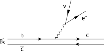
Figure 1: Diagrammatic representation of the quark level for $B_{c}\rightarrow\nu_{e}e^{-}(c\bar{c})$.

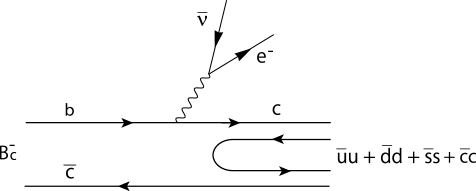
Figure 2: Dominant mechanism for the hadronization into two mesons of the $c\bar{c}$ state after the weak process.

The procedure followed here is inspired in the approach of Ref. Liang:2015twa where the basic mechanisms at the quark level are investigated, then pairs of hadrons are produced after implementing hadronization, and finally these hadrons are allowed to undergo final state interaction.

The hadronization of $c\bar{c}$, introducing the $q\bar{q}$ pair is done as follows   Liang:2015twa ; Navarra:2015iea . We take the $q\bar{q}$ matrix $M$,

$$M\equiv q\bar{q}^{\tau}=\left(\begin{array}[]{cccc}u\bar{u}&u\bar{d}&u\bar{s}&u\bar{c}\\ d\bar{u}&d\bar{d}&d\bar{s}&d\bar{c}\\ s\bar{u}&s\bar{d}&s\bar{s}&s\bar{c}\\ c\bar{u}&c\bar{d}&c\bar{s}&c\bar{c}\end{array}\right)$$ (5)

Then

$$c(\bar{u}u+\bar{d}d+\bar{s}s+\bar{c}c)\bar{c}=\sum_{i=1}^{4}M_{4i}M_{i4}=(M^{2})_{44}$$ (6)

We now write $M$ in terms of vector mesons and we have the vector matrix $V$,

$$M\rightarrow V\equiv\left(\begin{array}[]{cccc}\frac{\rho^{0}}{\sqrt{2}}+\frac{\omega}{\sqrt{2}}&\rho^{+}&K^{*+}&\bar{D}^{*0}\\ \rho^{-}&-\frac{\rho^{0}}{\sqrt{2}}+\frac{\omega}{\sqrt{2}}&K^{*0}&\bar{D}^{*-}\\ K^{*-}&\bar{K}^{*0}&\phi&\bar{D}_{s}^{*-}\\ D^{*0}&D^{*+}&D_{s}^{*+}&J/\psi\end{array}\right).$$ (11)

Then $M^{2}$ becomes $V^{2}$ and

$$(V\cdot V)_{44}=D^{*0}\bar{D}^{*0}+D^{*+}\bar{D}^{*-}+D^{*+}_{s}\bar{D}^{*-}_{s}+J/\psi J/\psi.$$ (12)

We neglect the $J/\psi J/\psi$ channel since it has too high energy relative to other channels. Only an $I=0$ state is produced from the $c\bar{c}$ component since the hadronization is a strong interaction and does not change isospin. We can write the $D^{*}\bar{D}^{*}$ combination in terms of the isospin doublets $(D^{*+},-D^{*0})$ and $(\bar{D}^{*0},\bar{D}^{*-})$ and then the production vertex is written as Liang:2015twa

$$(V\cdot V)_{44}\rightarrow\sqrt{2}|D^{*}\bar{D}^{*};I=0\rangle+|D^{*}_{s}\bar{D}^{*}_{s};I=0\rangle.$$ (13)

The final state interaction of $D^{*}\bar{D}^{*}$ is depicted in Fig. 3, and we use the interaction of Ref. Molina:2009ct where, using an extension of the local hidden gauge approach, the interaction of $D^{*}\bar{D}^{*}$ generates several resonances, and some $XYZ$ states were dynamically generated. As suggested in Refs. Liang:2015twa ; Molina:2009ct , the resonances most strongly coupled to the $D^{*}\bar{D}^{*}$ channel correspond to the experimental states $Y(3940),Z(3930)$ and the $D^{*}_{s}\bar{D}^{*}_{s}$ channel corresponds to the $X(4160)$.

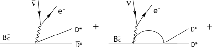
Figure 3: Diagrams involved in the final state interaction of the primary $D^{*}\bar{D^{*}}$ mesons, (a) tree level, (b) rescattering.

II.1 Coalescence

From the present perspective, we have studied the semileptonic decay process in Ref. Navarra:2015iea . First, we study the coalescence process which produces the resonances after rescattering, as shown in Fig. 4.

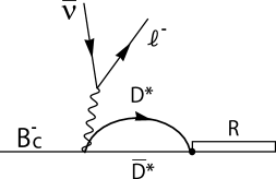
Figure 4: Diagrams of the coalescence process which produce the resonances after rescattering.

This process has a three-body final state with a lepton, its neutrino and the resonance $R$. The resonance $R$ stands for the $X,Y,Z$ resonances. The hadronization factor $V_{\rm had}$ can be obtained as

$$V_{\rm had}=C(\sqrt{2}\ G_{D^{*}\bar{D}^{*}}\ g_{R,D^{*}\bar{D}^{*}}+G_{D^{*}_{s}\bar{D}^{*}_{s}}\ g_{R,D^{*}_{s}\bar{D}^{*}_{s}}),$$ (14)

for the resonance $R$ in $J=0$ which requires $L=0$. For the constant $C$, we use the value $C=7.22$ of the semileptonic $B$ decays as established in Ref. Navarra:2015iea . $G_{D^{*}\bar{D}^{*}}$ and $G_{D^{*}_{s}\bar{D}^{*}_{s}}$ are the two meson loop functions, and $g_{R,D^{*}\bar{D}^{*}}$ and $g_{R,D^{*}_{s}\bar{D}^{*}_{s}}$ are the couplings of the resonance to these channels. We use the values reported in Ref. Molina:2009ct . The two meson loop function $G_{i}$ for each channel $i$ is

$$G_{i}(s)=i\int\frac{d^{4}q}{(2\pi)^{4}}\frac{1}{q^{2}-m_{1}^{2}+i\epsilon}\frac{1}{(P-q)^{2}-m_{2}^{2}+i\epsilon},$$ (15)

where $P$ is the total four-momentum of the two mesons, and $m_{1}$ and $m_{2}$ are the masses of the two mesons in channel $i$. We use cut off regularization as done in Wang:2017mrt to avoid potential problems of dimensional regularization pointed out in Wu:2010rv . The $G$ function has the form

$$G_{i}=\int^{q_{max}}_{0}\frac{q^{2}~{}dq}{(2\pi)^{2}}\dfrac{\omega_{1}+\omega_{2}}{\omega_{1}~{}\omega_{2}\Big{(}(P^{0})^{2}-(\omega_{1}+\omega_{2})^{2}+i~{}\epsilon\Big{)}},$$ (16)

where $q_{max}$ stands for the cutoff in the three momentum, the square of center of mass energy $(P^{0})^{2}=s$ and $\omega_{i}=\sqrt{\vec{q}^{~{}2}_{i}+m^{2}_{i}}$. As in Wang:2017mrt we use $q_{max}=690$ MeV.

The whole amplitude $T_{B_{c}}$ for the semileptonic decay of the $B_{c}$ meson is written as,

$$T_{B_{c}}=-i\frac{G_{\rm F}V_{bc}}{\sqrt{2}}L^{\alpha}Q_{\alpha}V_{\rm had},$$ (17)

where

$$L^{\alpha}=\bar{u}_{\nu}\gamma^{\alpha}(1-\gamma_{5})v_{l},\hskip 8.53581ptQ_{\alpha}=\bar{u}_{c}\gamma_{\alpha}(1-\gamma_{5})u_{b}.$$ (18)

By following the steps of Refs. Navarra:2015iea ; Sekihara:2015iha , we find for the sum and average over the polarization of the fermions

$$\frac{1}{2}\sum_{\rm pol}|T_{B_{c}}|^{2}=\frac{4|G_{\rm F}V_{bc}V_{\rm had}|^{2}}{m_{e}m_{\nu}m_{B_{c}}m_{R}}(p_{B_{c}}\cdot p_{\nu})(p_{R}\cdot p_{e}).$$ (19)

Further steps are done in Ref. Navarra:2015iea to perform the angular integrations of the resonance in the $B_{c}$ rest frame and the lepton in the $\nu e$ rest frame, and finally one obtains a formula of the decay widths $\Gamma_{\rm coal}$ for the coalescence of the $X,Y,Z$ resonances by

$$\Gamma_{\rm coal} = \frac{|G_{\rm F}V_{bc}V_{{\rm had}}|^{2}}{8\pi^{3}m_{B_{c}}^{3}m_{R}}$$

$$\times \int dM_{\rm inv}^{(\nu e)}P^{\rm cm}_{R}\tilde{p}_{\nu}|M_{\rm inv}^{(\nu e)}|^{2}\left(\tilde{E}_{B_{c}}\tilde{E}_{R}-\frac{\tilde{p}_{B_{c}}^{2}}{3}\right).$$

Here, $P^{\rm cm}_{R}$ is the momentum of the resonance $R$ in the $B_{c}$ rest frame, and $\tilde{p}_{\nu}$ is the momentum of the neutrino in the $\nu e$ rest frame,

$$P^{\rm cm}_{R} = \frac{\lambda^{1/2}(m_{B_{c}}^{2},[M_{\rm inv}^{(\nu e)}]^{2},m_{R}^{2})}{2m_{B_{c}}},$$ (21)

$$\tilde{p}_{\nu} = \frac{\lambda^{1/2}([M_{\rm inv}^{(\nu e)}]^{2},m_{\nu}^{2},m_{e}^{2})}{2M_{\rm inv}^{(\nu e)}},$$ (22)

with the Källen function defined as,

$$\lambda(a,b,c)=a^{2}+b^{2}+c^{2}-2ab-2bc-2ca.$$ (23)

The energies $\tilde{E}_{B_{c}}$ and $\tilde{E}_{R}$ are calculated in the $\nu e$ rest frame,

$$\tilde{E}_{B_{c}} = \frac{m_{B_{c}}^{2}+[M_{\rm inv}^{(\nu e)}]^{2}-m_{R}^{2}}{2M_{\rm inv}^{(\nu e)}},$$ (24)

$$\tilde{E}_{R} = \frac{m_{B_{c}}^{2}-[M_{\rm inv}^{(\nu e)}]^{2}-m_{R}^{2}}{2M_{\rm inv}^{(\nu e)}},$$ (25)

and $\tilde{p}_{B_{c}}$ is the momentum of the $B_{c}$ in the $\nu e$ rest frame,

$$\tilde{p}_{B_{c}}^{2} = \tilde{E}_{B_{c}}^{2}-m_{B_{c}}^{2}.$$ (26)

The integral range of $M_{\rm inv}^{(\nu e)}$ is $[m_{e}+m_{\nu},m_{B_{c}}-m_{R}]$. We take the Fermi coupling constant $G_{\rm F}=1.166\times 10^{-5}$ GeV^-2 and the Cabibbo-Kobayashi-Maskawa matrix element $V_{bc}=0.0411$.

For the other resonance of $2^{++}$, we can not use the formula in Eq. (LABEL:eq:dGam) because we need $L=2$ state and hence the matrix element would be different. For the $L=2$ case we replace the $P^{\rm cm}_{R}$ with $(P^{\rm cm}_{R})^{5}$ in Eq. LABEL:eq:dGam, but we do not obtained an absolute value for the width. Yet, we can obtain the ratio of rates for the two $2^{++}$ resonances.

II.2 Rescattering

Next, we study the rescattering in the final states $D^{*}\bar{D^{*}}$ and $D_{s}^{*}\bar{D_{s}^{*}}$ as shown in Fig. 3. The different final states of the $D^{*}\bar{D^{*}}$ and $D_{s}^{*}\bar{D_{s}^{*}}$ are treated separately. The amplitude $V_{\rm had}^{\prime}$ in the $D^{*}\bar{D^{*}}$ states for $I=0,~{}J=0$ and $I=0,~{}J=2$, where the resonances couple strongly to $D^{*}\bar{D^{*}}$, is written as,

$$V_{\rm had}^{\prime} = C(\sqrt{2}+\sqrt{2}\ G_{D^{*}\bar{D}^{*}}\ t_{D^{*}\bar{D}^{*},D^{*}\bar{D}^{*}}$$ (27)

$$+\ G_{D_{s}^{*}\bar{D}_{s}^{*}}\ t_{D^{*}_{s}\bar{D}^{*}_{s},D^{*}\bar{D}^{*}}).$$

where $G$ is the two meson loop function for each channel in Eq. (16). The factor $C$ is not the same for $J=0$ and $J=2$, and we will come back to that.

On the other hand, in the other case of resonance coupled to the $D_{s}^{*}\bar{D_{s}^{*}}$ state for $I=0,J=2$, the hadronization amplitude $V^{\prime}_{\rm had}$ is written as,

$$V_{\rm had}^{\prime} = C^{\prime}(1+\sqrt{2}\ G_{D^{*}\bar{D}^{*}}\ t_{D^{*}\bar{D}^{*},D^{*}_{s}\bar{D}^{*}_{s}}$$ (28)

$$+\ G_{D_{s}^{*}\bar{D}_{s}^{*}}\ t_{D^{*}_{s}\bar{D}^{*}_{s},D^{*}_{s}\bar{D}^{*}_{s}}).$$

The scattering amplitudes $t_{D^{*}\bar{D}^{*},D^{*}\bar{D}^{*}}$, $t_{D^{*}_{s}\bar{D}^{*}_{s},D^{*}\bar{D}^{*}}$ and $t_{D^{*}_{s}\bar{D}^{*}_{s},D^{*}_{s}\bar{D}^{*}_{s}}$ for the $D^{*}\bar{D}^{*}\rightarrow D^{*}\bar{D}^{*}$, $D^{*}\bar{D}^{*}\rightarrow D^{*}_{s}\bar{D}^{*}_{s}$, and $D^{*}_{s}\bar{D}^{*}_{s}\rightarrow D^{*}_{s}\bar{D}^{*}_{s}$ transitions are written as

$$t_{D^{*}\bar{D}^{*},D^{*}\bar{D}^{*}} = \frac{g_{R,D^{*}\bar{D}^{*}}g_{R,D^{*}\bar{D}^{*}}}{M^{2}_{\rm inv}-M_{R}^{2}+iM_{R}\Gamma_{R}},$$ (29)

$$t_{D^{*}_{s}\bar{D}^{*}_{s},D^{*}\bar{D}^{*}} = \frac{g_{R,D^{*}_{s}\bar{D}^{*}_{s}}g_{R,D^{*}\bar{D}^{*}}}{M_{\rm inv}^{2}-M_{R}^{2}+iM_{R}\Gamma_{R}},$$ (30)

$$t_{D^{*}_{s}\bar{D}^{*}_{s},D^{*}_{s}\bar{D}^{*}_{s}} = \frac{g_{R,D^{*}_{s}\bar{D}^{*}_{s}}g_{R,D^{*}_{s}\bar{D}^{*}_{s}}}{M_{\rm inv}^{2}-M_{R}^{2}+iM_{R}\Gamma_{R},}$$ (31)

where $M_{\rm inv}$ in the denominator refers to the final $D^{*}\bar{D}^{*}$ or $D^{*}_{s}\bar{D}^{*}_{s}$ states. The scattering amplitude $t_{D^{*}_{s}\bar{D}^{*}_{s},D^{*}\bar{D}^{*}}$ is the same as the $t_{D^{*}\bar{D}^{*},D^{*}_{s}\bar{D}^{*}_{s}}$ one. The coupling constants $g_{i}$ are the same as in Eq. (14).

The differential decay widths $\displaystyle\frac{d\Gamma}{dM_{\rm inv}}$ are given by Navarra:2015iea ; Sekihara:2015iha ; Ikeno:2015xea

$$\frac{d\Gamma_{i}}{dM_{\rm inv}} = \frac{|G_{\rm F}V_{bc}V^{\prime}_{{\rm had},i}|^{2}}{32\pi^{5}m_{B_{c}}^{3}M_{\rm inv}^{(i)}}$$

$$\times \int dM_{\rm inv}^{(\nu e)}P^{\rm cm}\tilde{p}_{\nu}\tilde{p}_{i}M_{\rm inv}^{(\nu e)^{2}}\left(\tilde{E}_{B_{c}}\tilde{E}_{i}-\frac{\tilde{p}_{B_{c}}^{2}}{3}\right)$$

where $i$ corresponds to the $D^{*}\bar{D}^{*}$ or $D^{*}_{s}\bar{D}^{*}_{s}$ states. In the case of the $L=2$ state, we replace $P^{\rm cm}$ by $(P^{\rm cm})^{5}$ as done before in the integrand of Eq. (LABEL:eq:dGam) for the coalescence case. Here, $P^{\rm cm}$ is the momentum of the $\nu e$ system in the $B_{c}$ rest frame, $\tilde{p}_{\nu}$ is the momentum of the neutrino in the $\nu e$ rest frame as defined in Eq. (22), and $\tilde{p}_{i}$ is the relative momentum of the final mesons in their rest frame,

$$P^{\rm cm} = \frac{\lambda^{1/2}(m_{B_{c}}^{2},[M_{\rm inv}^{(\nu e)}]^{2},[M_{\rm inv}^{(i)}]^{2})}{2m_{B_{c}}},$$ (33)

$$\tilde{p}_{i} = \frac{\lambda^{1/2}([M_{\rm inv}^{(i)}]^{2},m_{i}^{2},m_{i}^{\prime 2})}{2M_{\rm inv}^{(i)}},$$ (34)

with $m_{i}$, $m_{i}^{\prime}$ the two meson masses of the final state. The energies $\tilde{E}_{B_{c}}$ and $\tilde{E}_{i}$ are calculated in the $\nu e$ rest frame,

$$\tilde{E}_{B_{c}} = \frac{m_{B_{c}}^{2}+[M_{\rm inv}^{(\nu e)}]^{2}-[M_{\rm inv}^{(i)}]^{2}}{2M_{\rm inv}^{(\nu e)}},$$ (35)

$$\tilde{E}_{i} = \frac{m_{B_{c}}^{2}-[M_{\rm inv}^{(\nu e)}]^{2}-[M_{\rm inv}^{(i)}]^{2}}{2M_{\rm inv}^{(\nu e)}}.$$ (36)

and $\tilde{p}_{B_{c}}$ is given by Eq. (26).

III Results

First, we show the results of the coalescence process. We consider $X(3934)$ as the resonance $R$, namely the $B^{-}_{c}\rightarrow X(3934)\bar{\nu}l^{-}$ process. We evaluate the decay widths $\Gamma_{\rm coal}$ in Eq.(LABEL:eq:dGam) for the resonance $L=0$ and $J=0$ state using the mass $m_{R}=3943$ MeV, and find

$$\Gamma_{\rm coal}=2.6\times 10^{-14}~{}{\rm MeV}.$$ (37)

In Fig. 5 we show the integrand of Eq. (LABEL:eq:dGam). The mean life of the $B_{c}$ is $0.507\times 10^{-12}$ s, and then the branching ratio is evaluated as

$$\frac{\Gamma_{\rm coal}}{\Gamma_{\rm tot}(B_{c})}=2.0\times 10^{-5}.$$ (38)

Figure 5: The integrand of the integral that appears in Eq. (LABEL:eq:dGam) as a function $M_{\rm inv}^{(\nu e)}$ for the resonance mass $X(3940)$ of $M_{R}=3943$ MeV.

For the other resonance of $2^{++}$, we can not use the formula of the decay widths in Eq. (LABEL:eq:dGam) because we need an $L=2$ state and hence the matrix element would be different. Thus, we calculated the ratio of the two $L=2$. We consider two options. In the first one the ratio is evaluated as,

$$\frac{\Gamma_{\rm coal}(2)}{\Gamma_{\rm coal}(2^{\prime})}=\frac{|V_{\rm had}(2)|^{2}/m_{R}(2)}{|V_{\rm had}(2^{\prime})|^{2}/m_{R}(2^{\prime})}=1.6$$ (39)

where $(2)$ indicates the $X(3930)$ resonance state of the mass $m_{R}=3922$ MeV, and $(2)^{\prime}$ the $X(4160)$ resonance state of the $m_{R}=4169$ MeV.

For the other option, we consider that the integral in Eq. (LABEL:eq:dGam) would have a different form to account for $L=2$,

$$\int dM_{\rm inv}^{(\nu e)}(P^{\rm cm}_{R})^{5}\tilde{p}_{\nu}|M_{\rm inv}^{(\nu e)}|^{2}\left(\tilde{E}_{B_{c}}\tilde{E}_{R}-\frac{\tilde{p}_{B_{c}}^{2}}{3}\right).$$ (40)

By replacing the integral in Eq. (LABEL:eq:dGam) by Eq. (40), the other ratio is evaluated as

$$\frac{\Gamma_{\rm coal}(2)}{\Gamma_{\rm coal}(2^{\prime})}=3.6$$ (41)

This latter result is more realistic and we take it. We also show the integrand of Eq. (40) in Fig. 6 for the two tensor resonances.

Figure 6: The integrands of the integral that appears in Eq. (40) as a function $M_{\rm inv}^{(\nu e)}$ for the resonance mass $X(3930)$ of $M_{R}=3922$ MeV and the resonance mass $X(4160)$ of $M_{R}=4169$ MeV.

Next, we show the results for the rescattering process. In order to study the rescattering process the scattering amplitudes $t_{D^{*}\bar{D}^{*},D^{*}\bar{D}^{*}}$, $t_{D^{*}_{s}\bar{D}^{*}_{s},D^{*}\bar{D}^{*}}$ and $t_{D^{*}_{s}\bar{D}^{*}_{s},D^{*}_{s}\bar{D}^{*}_{s}}$ are needed. We use the amplitudes of Eqs. (29), (30) and (31). In Fig. 7, using Eqs. (LABEL:eq:dGam) and (LABEL:eq:dGamR), we show the result for $\frac{M_{R}}{\Gamma_{\rm coal}}\frac{d\Gamma_{i}}{dM_{\rm inv}}$ as a function of $M_{inv}(D^{*}\bar{D}^{*})$ for the $B^{-}_{c}\rightarrow\bar{\nu}_{l}l^{-}X(3940)$ decay, where the dashed line corresponds to a phase space distribution which we normalize to the same area in the range of the figure. As we can see from Fig. 7, the shape of $D^{*}\bar{D}^{*}$ invariant mass distribution is different from the phase space.

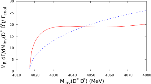
Figure 7: The $\frac{M_{R}}{\Gamma_{\rm coal}}\frac{d\Gamma_{i}}{dM_{\rm inv}}$ as a function of $M_{inv}(D^{*}\bar{D}^{*})$ for the $B_{c}\rightarrow\nu_{l}l^{+}Y(3940)$ decay. The dashed line corresponds to phase space.

We have also evaluated $\frac{M_{R}}{\Gamma_{\rm coal}}\frac{d\Gamma_{i}}{dM_{\rm inv}}$ for the $B^{-}_{c}\rightarrow\bar{\nu}_{l}l^{-}X(3930)$ decay. The result is depicted as a function of $M_{inv}(D^{*}\bar{D}^{*})$ in Fig. 8. The dash curve in this figure is the phase space. The difference with phace space is also apparent.

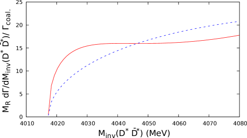
Figure 8: The $\frac{M_{R}}{\Gamma_{\rm coal}}\frac{d\Gamma_{i}}{dM_{\rm inv}}$ as a function of $M_{inv}(D^{*}\bar{D}^{*})$ for the $B_{c}\rightarrow\nu_{l}l^{+}Z(3930)$ decay. The dashed line corresponds to phase space.

Finally, we show the result for the $B^{-}_{c}\rightarrow\bar{\nu}_{l}l^{-}X(4160)$ decay in Fig. 9 as a function of the $D^{*}_{s}\bar{D}^{*}_{s}$ mass distribution. We observe in this case that the mass distribution close to the $D^{*}_{s}\bar{D}^{*}_{s}$ is quite different from the phace space.

As important as the shape, showing the presence of a resonance below threshold, the values in the scale, corresponding to ratios, are absolute values of our predictions, tied to the molecular nature of these resonances and their strong coupling to $D^{*}\bar{D}^{*}$ and $D^{*}_{s}\bar{D}^{*}_{s}$. We should note that we have compared the $D^{*}\bar{D}^{*}$ or $D^{*}_{s}\bar{D}^{*}_{s}$ production with the production of each particular resonance. This implies that in the experiment the $S$-wave is separated from the $D$-wave in each case, something that is at reach in present partial wave analysis of data Aaij:2016nsc ; Aaij:2015tga

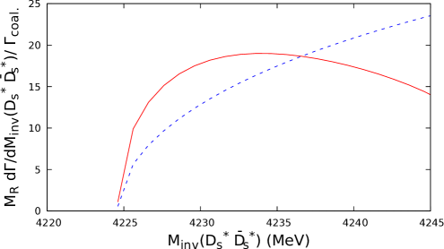
Figure 9: The $\frac{M_{R}}{\Gamma_{\rm coal}}\frac{d\Gamma_{i}}{dM_{\rm inv}}$ as a function of $M_{inv}(D^{*}_{s}\bar{D}^{*}_{s})$ for the $B_{c}\rightarrow\nu_{l}l^{+}X(4160)$ decay. The dashed line corresponds to phase space.

IV Conclusions

We have studied the semileptonic decay of $B_{c}$ in the reaction $B^{-}_{c}\rightarrow\bar{\nu}_{e}e^{-}X$, with $X$ any of the resonances $X(3930)~{}(2^{++})$, $X(3940)~{}(0^{++})$ and $X(4160)~{}(2^{++})$. The main point of the approach is that we treat these resonances as dinamically generated from the vector-vector interaction in the charm sector.

The $X(3940)$ and $X(3930)$ states are basically $D^{*}\bar{D}^{*}$ molecules in that approach, although they also couple to other channels with a smaller intensity. To produce these $X$ states one proceeds in three steps. The first one looks into the elementary process $B^{-}_{c}\rightarrow\bar{\nu}_{e}e^{-}c\bar{c}$. In the second step the $c\bar{c}$ pair hadronizes producing an extra $\bar{q}q$ with the vacuum quantum numbers, which leads to $D^{*}\bar{D}^{*}$ and $D^{*}_{s}\bar{D}^{*}_{s}$ pairs. In the last step these mesons are allowed to undergo final state interaction from where the three resonances appear. By analogy with other reactions producing scalar mesons in the final state, we make an estimation of the rate of $B^{-}_{c}\rightarrow\bar{\nu}_{e}e^{-}X(3940)$. For the production of the two tensor states we can not obtain the absolute rate of production, but we can obtain the ratio for the $X(3930)$ and $X(4160)$ states. We also look at the production of $D^{*}\bar{D}^{*}$ and $D^{*}_{s}\bar{D}^{*}_{s}$ close to threshold and we can make predictions of the ratio of this differential mass distribution to the rate of resonance production, which are tied to the nature of these resonances as dynamically generated from the vector-vector interaction in the charm sector. As more decay modes of $B_{c}$ become available, it would be interesting to look into these modes which will provide good information on the nature of these resonances.

References

- [1] S. Godfrey and N. Isgur, Phys. Rev. D 32, 189 (1985).
- [2] J. Vijande, F. Fernandez and A. Valcarce, J. Phys. G 31, 481 (2005).
- [3] H. X. Chen, W. Chen, X. Liu and S. L. Zhu, Phys. Rept. 639, 1 (2016).
- [4] X. Liu, Chin. Sci. Bull. 59, 3815 (2014).
- [5] S. Godfrey and S. L. Olsen, Ann. Rev. Nucl. Part. Sci. 58, 51 (2008).
- [6] F. K. Guo, C. Hanhart, U. G. Meißner, Q. Wang, Q. Zhao and B. S. Zou, arXiv:1705.00141 [hep-ph].
- [7] H. X. Chen, E. L. Cui, W. Chen, X. Liu and S. L. Zhu, Eur. Phys. J. C 77, no. 3, 160 (2017).
- [8] A. Esposito, A. Pilloni and A. D. Polosa, Phys. Rept. 668, 1 (2016).
- [9] P. G. Ortega, D. R. Entem and F. Fernandez, J. Phys. G 40, 065107 (2013).
- [10] R. Molina and E. Oset, Phys. Rev. D 80, 114013 (2009).
- [11] M. Bando, T. Kugo and K. Yamawaki, Phys. Rept. 164, 217 (1988).
- [12] M. Harada and K. Yamawaki, Phys. Rept. 381, 1 (2003).
- [13] U. G. Meissner, Phys. Rept. 161, 213 (1988).
- [14] K. Abe et al. [Belle Collaboration], Phys. Rev. Lett. 94, 182002 (2005).
- [15] K. Abe et al. [Belle Collaboration], Phys. Rev. Lett. 98, 082001 (2007).
- [16] S. Uehara et al. [Belle Collaboration], Phys. Rev. Lett. 96, 082003 (2006).
- [17] C. Patrignani et al. [Particle Data Group], Chin. Phys. C 40, no. 10, 100001 (2016).
- [18] Z. Y. Zhou, Z. Xiao and H. Q. Zhou, Phys. Rev. Lett. 115, no. 2, 022001 (2015).
- [19] P. G. Ortega, J. Segovia, D. R. Entem and F. Fernandez, arXiv:1706.02639 [hep-ph].
- [20] P. Pakhlov et al. [Belle Collaboration], Phys. Rev. Lett. 100, 202001 (2008).
- [21] X. Liu and S. L. Zhu, Y(4143) is probably a molecular partner of Y(3930), Phys. Rev. D 80, 017502 (2009) Erratum: [Phys. Rev. D 85, 019902 (2012)].
- [22] T. Branz, T. Gutsche and V. E. Lyubovitskij, Hadronic molecule structure of the Y(3940) and Y(4140), Phys. Rev. D 80, 054019 (2009).
- [23] S. Weinberg, Evidence That the Deuteron Is Not an Elementary Particle, Phys. Rev. 137, B672 (1965).
- [24] V. Baru, J. Haidenbauer, C. Hanhart, Y. Kalashnikova and A. E. Kudryavtsev, Evidence that the a(0)(980) and f(0)(980) are not elementary particles, Phys. Lett. B 586, 53 (2004).
- [25] X. Chen, X. Lü, R. Shi and X. Guo, arXiv:1512.06483 [hep-ph].
- [26] M. Karliner and J. L. Rosner, Exotic resonances due to exchange, Nucl. Phys. A 954, 365 (2016).
- [27] R. M. Albuquerque, M. E. Bracco and M. Nielsen, A QCD sum rule calculation for the Y(4140) narrow structure, Phys. Lett. B 678, 186 (2009).
- [28] J. R. Zhang and M. Q. Huang, (Q anti-s)(*)(anti-Qs)(*) molecular states from QCD sum rules: A view on Y(4140), J. Phys. G 37, 025005 (2010).
- [29] R. Aaij et al. [LHCb Collaboration], Phys. Rev. Lett. 118, no. 2, 022003 (2017).
- [30] R. Aaij et al. [LHCb Collaboration], Phys. Rev. D 95, no. 1, 012002 (2017).
- [31] T. Aaltonen et al. [CDF Collaboration], Phys. Rev. Lett. 102, 242002 (2009).
- [32] J. Brodzicka, Conf. Proc. C 0908171, 299 (2009).
- [33] T. Aaltonen et al. [CDF Collaboration], Mod. Phys. Lett. A 32, no. 26, 1750139 (2017).
- [34] R. Aaij et al. [LHCb Collaboration], Phys. Rev. D 85, 091103 (2012).
- [35] S. Chatrchyan et al. [CMS Collaboration], Phys. Lett. B 734, 261 (2014).
- [36] V. M. Abazov et al. [D0 Collaboration], Phys. Rev. D 89, no. 1, 012004 (2014).
- [37] J. P. Lees et al. [BaBar Collaboration], Phys. Rev. D 91, no. 1, 012003 (2015).
- [38] V. M. Abazov et al. [D0 Collaboration], Phys. Rev. Lett. 115, no. 23, 232001 (2015).
- [39] E. Wang, J. J. Xie, L. S. Geng and E. Oset, Phys. Rev. D 97, 014017 (2018).
- [40] J. J. Wu and B. S. Zou, Phys. Lett. B 709, 70 (2012).
- [41] Z. H. Wang, Y. Zhang, T. h. Wang, Y. Jiang and G. L. Wang, J. Phys. G 43, no. 10, 105002 (2016). {ö
- [42] F. S. Navarra, M. Nielsen, E. Oset and T. Sekihara, Phys. Rev. D 92, no. 1, 014031 (2015).
- [43] T. Sekihara and E. Oset, Phys. Rev. D 92, 054038 (2015).
- [44] N. Ikeno and E. Oset, Phys. Rev. D 93, 014021 (2016).
- [45] W. H. Liang, E. Oset and Z. S. Xie, Phys. Rev. D 95, no. 1, 014015 (2017).
- [46] W. H. Liang, T. Uchino, C. W. Xiao and E. Oset, Eur. Phys. J. A 51, no. 2, 16 (2015).
- [47] W. H. Liang, J. J. Xie, E. Oset, R. Molina and M. Doring, Eur. Phys. J. A 51, 58 (2015).
- [48] R. Aaij et al. [LHCb Collaboration], Phys. Rev. Lett. 115, 072001 (2015).