$\mathcal{PT}$-symmetric and antisymmetric nonlinear states in a split potential box

Abstract

We introduce a one-dimensional $\mathcal{PT}$-symmetric system, which includes the cubic self-focusing, a double-well potential in the form of an infinitely deep potential box split in the middle by a delta-functional barrier of an effective height $\varepsilon$, and constant linear gain and loss, $\gamma$, in each half-box. The system may be readily realized in microwave photonics. Using numerical methods, we construct $\mathcal{PT}$-symmetric and antisymmetric modes, which represent, respectively, the system’s ground state and first excited state, and identify their stability. Their instability mainly leads to blowup, except for the case of $\varepsilon=0$, when an unstable symmetric mode transforms into a weakly oscillating breather, and an unstable antisymmetric mode relaxes into a stable symmetric one. At $\varepsilon>0$, the stability area is much larger for the $\mathcal{PT}$-antisymmetric state than for its symmetric counterpart. The stability areas shrink with with increase of the total power, $P$. In the linear limit, which corresponds to $P\rightarrow 0$, the stability boundary is found in a analytical form.The stability area of the antisymmetric state originally expands with the growth of $\gamma$, and then disappears at a critical value of $\gamma$.

I Introduction

Although the quantum theory operates complex wave functions, a fundamental principle is that eigenvalues of physically relevant quantities must be real. Normally, this condition is satisfied if the underlying Hamiltonian is Hermitian qm . However, it was discovered that Hamiltonians composed of Hermitian and anti-Hermitian parts, subject to the constraint of the parity-time ($\mathcal{PT}$) symmetry, also generate real energy spectra, provided that the strength of the anti-Hermitian part does not exceed a certain critical value, above which the $\mathcal{PT}$ symmetry breaks down, i.e., the energy spectra ceases to be real bender1 -review2 . For one-dimensional single-particle Hamiltonians, which include a complex potential, $U(x)=V(x)+iW(x)$, whose imaginary part is the anti-Hermitian term in the Hamiltonian, the $\mathcal{PT}$ symmetry implies that the real and imaginary parts of the potential are, respectively, even and odd functions of the coordinate bender1 :

$$V(x)=V(-x),W(-x)=-W(x).$$ (1)

While the concept of $\mathcal{PT}$-symmetric Hamiltonians was not experimentally realized in the framework of the quantum theory, a possibility was proposed to emulate the symmetry in optical media with symmetrically placed gain and loss elements theo1 -Kominis , making use of the commonly known similarity between the Schrödinger equation in quantum mechanics and the equation governing light propagation in the paraxial approximation. In fact, this setting may be considered as a specific example of the general class of dissipated structures, the concept of which was developed by I. Prigogine and his collaborators Prig . This prediction was followed by the experimental implementation of the $\mathcal{PT}$ symmetry in various optical waveguides exp1 -exp7 and lasers exp5 ; Longhi , as well as in other photonic settings, such as metamaterials exp4 , microcavities exp6 , optically induced atomic lattices exp8 , and exciton-polariton condensates exci1 -exci3 .

The $\mathcal{PT}$ symmetry can be emulated in other waveguiding settings too, such as acoustics acoustics1 ; acoustics2 , optomechanical systems om , and electronic circuits electronics . It was predicted too in atomic Bose-Einstein condensates (BECs) Cartarius and magnetism magnetism . In terms of the theory, $\mathcal{PT}$-symmetric extensions were also elaborated for Korteweg - de Vries KdV1 ; KdV2 , Burgers Zhenya-Burgers , and sine-Gordon Cuevas equations, as well as in a model combining the $\mathcal{PT}$ symmetry with emulation of the spin-orbit coupling in optics HS .

While the $\mathcal{PT}$ symmetry is a linear property, it may be combined with intrinsic nonlinearity of the medium in which the symmetry is implemented, which is usually as the Kerr self-focusing of optical materials. Usually, such settings are modelled by nonlinear Schrödinger (NLS) equations with complex potentials subject to constraint (1). In particular, these models give rise to $\mathcal{PT}$-symmetric solitons, which were considered in a large number of works soliton , Konotop -unbreakable (see recent reviewed in Refs. review1 and PT-review2 ), and experimentally demonstrated too exp7 . A characteristic feature of $\mathcal{PT}$-symmetric solitons and other nonlinear modes is that they form continuous families, like in conservative systems families , although the $\mathcal{PT}$-symmetry is realized in dissipative media. In that sense, $\mathcal{PT}$-symmetric systems represent an interface between conservative models and traditional dissipative ones, which normally give rise to isolated solutions in the form of dissipative solitons, which do not form families diss1 -diss3 .

The objective of the present work is to introduce a one-dimensional model which combines the $\mathcal{PT}$ symmetry and cubic self-focusing at the most basic level. As concerns the spatially even real part of the potential, $V(x)$ in Eq. (1), its most fundamental version is represented by the double-well structure DWP1 -DWP4, book . In turn, what may be considered as, arguably, the most basic form of such a potential in one dimension is a infinitely deep potential box, split in the middle (at $x=0$) by an infinitely narrow delta-functional barrier NatPhot ; Elad . In this work, we combine the real split-box potential with the simplest imaginary one, represented by constant gain and loss coefficients in two half-boxes, at $x>0$ and $x<0$, respectively. Microwave photonics, which may involve cubic nonlinearity (see, e.g., Ref. Slavin ), offers the most straightforward possibility to implement this complex potential, with the box realized as a waveguide with metallic walls, and the central splitter induced by a metallic strip partly separating the guiding channel in two micro . The symmetric gain and loss may be realized, in the lossy material filling the waveguide, by installing an amplifier, with an appropriate value of the gain, at $x>0$. In principle, the same model may be implemented in BEC too, assuming that the condensate is loaded into an appropriately shaped trapping potential, with symmetrically placed amplifying and lossy elements Cartarius , but this may be difficult to achieve in the real experiment.

The model is formulated in detail in Section II. Then, in Section III, we report an analytically derived stability boundary for the zero state in the linearized version of the model, which is a nontrivial finding in the presence of the complex potential. The main problem, which is addressed in Section IV, is constructing nonlinear $\mathcal{PT}$-symmetric and antisymmetric states in this system [alias the ground state (GS), and the first excited state, respectively]. This is done by means of numerical methods (the imaginary-time integration for the GS, and the Newton’s method for the antisymmetric modes). Further, we focus on identifying existence and stability boundaries of these states. In particular, a noteworthy finding is that the stability area is much larger for the antisymmetric state than for the symmetric one. The paper is concluded by Section V.

II The model

We consider a 1D model based on the $\mathcal{PT}$-symmetric NLS equation with the cubic self-focusing nonlinearity term, a double-well potential, in the form of the infinitely deep box, split in the middle by the delta-functional barrier, and uniform gain and loss applied in two half-boxes. The NLS equation is written in the normalized form with zero boundary conditions at edges of the box, $x=\pm 1/2$:

$$i\frac{\partial\psi}{\partial z}=-\frac{1}{2}\frac{\partial^{2}\psi}{\partial x^{2}}-g\left|\psi\right|^{2}\psi+\varepsilon\delta(x)\psi+i\gamma\sigma(x)\psi,$$ (2)

$$\psi\left(x=\pm\frac{1}{2}\right)=0.$$ (3)

Here $z$ and $x$ are the propagation distance and transverse coordinate in the waveguide, which take values, respectively, $z\geq 0$ and $|x|\,\leq 1/2$ (i.e., the width of the waveguide is scaled to be $1$). Further, $\varepsilon$ is the strength of the splitting barrier, and the self-focusing coefficient is normalized to be $g=1$, except for $g=0$ in the linearized model. Coefficient $\gamma$ in Eq. (2) represents the strength of gain-loss term, with $\sigma(x)$ being an odd function of $x$, which we here chose as the step profile:

$$\sigma(x)=\mathrm{sgn}(x).$$ (4)

Stationary solutions to Eq. (2) are looked for as

$$\psi(x,z)=\exp\left(ikz\right)u(x),$$ (5)

where $k$ is a real propagation constant, and complex function $u$ satisfies equations

$$-ku+\frac{1}{2}\frac{d^{2}u}{dx^{2}}+g\left|u\right|^{2}u=\varepsilon\delta(x)u+i\gamma\mathrm{sgn}(x)u,$$ (6)

$$u\left(x=\pm\frac{1}{2}\right)=0.$$ (7)

Stationary states are characterized by the the total power,

$$P=\int_{-1/2}^{+1/2}|\psi(x)|^{2}dx$$ (8)

To analyze stability of stationary states, we search for perturbed solutions to Eq. (2) as

$$\psi(x,z)=e^{ikz}[u(x)+v_{1}(x)e^{-i\lambda z}+v_{2}^{\ast}(x)e^{i\lambda^{\ast}z}]$$ (9)

where $v_{1}(x)$ and $v_{2}(x)$ are infinitesimal perturbation eigenmodes, and $\lambda$ is the respective instability growth rate. Linearization around the stationary solutions leads to the following equation:

$$\left(\begin{array}[]{cc}\hat{F}+i\gamma\sigma(x)&-u^{2}\\ (u^{\ast})^{2}&-\hat{F}+i\gamma\sigma(x)\end{array}\right)\left(\begin{array}[]{c}v_{1}\\ v_{2}\end{array}\right)=\lambda\left(\begin{array}[]{c}v_{1}\\ v_{2}\end{array}\right),$$ (10)

where $\hat{F}=-(1/2)d^{2}/dx^{2}-2\left|u\right|^{2}+\epsilon\delta(x)+k$. This equation, with boundary conditions (7), were solved numerically. The instability is predicted by the existence of eigenvalues with $\mathrm{Im}(\lambda)\neq 0$.

III Analytical results: stability of the zero background

The first objective of the analysis is stability of the zero solution in the framework of the present model, which is a nontrivial issue in the presence of the complex potential. The corresponding eigenmodes and eigenvalues $k$ should be found from the linearized version of Eqs. (6):

$$-ku+\frac{1}{2}\frac{d^{2}u}{dx^{2}}=\varepsilon\delta(x)u+i\gamma\mathrm{sgn}(x)u,$$ (11)

the stability implying that $k$ must be real. $\mathcal{PT}$-symmetric solutions to Eq. (11) are singled out by condition

$$u(-x)=u^{\ast}(x),$$ (12)

with $\ast$ standing for the complex conjugation. Accordingly, the solutions are looked for as

$$u(x)=v(x)+iw(x),$$ (13)

with the real and imaginary parts subject to the following constraints:

$$v(-x)=v(x),~{}w(-x)=-w(x).$$ (14)

At $x\neq 0$, where $\delta(x)$ does not appear in Eq. (11), one can eliminate $v$ in favor of $w$ in Eq. (11), after the substitution of expression (13), and thus derive a single equation for $w(x)$:

$$v(x)=\frac{\mathrm{sgn}(x)}{\gamma}\left(-kw+\frac{1}{2}\frac{d^{2}w}{dx^{2}}\right),$$ (15)

$$\frac{1}{4}\frac{d^{4}w}{dx^{2}}-k\frac{d^{2}w}{dx^{2}}+\left(k^{2}+\gamma^{2}\right)w=0$$ (16)

Fundamental solutions to Eq. (16) [which, for the time being, do not take boundary conditions (7) into regard] are looked for in an obvious form:

$$u=\mathrm{const}\cdot\exp\left(Qx\right),$$ (17)

$$Q^{2}=2\left(k\pm i\gamma\right).$$ (18)

Equation (18) yields four roots:

$$Q = \pm Q_{r}\oplus iQ_{i},$$ (19)

$$Q_{r} \equiv \sqrt{\sqrt{k^{2}+\gamma^{2}}+k},$$ (20)

$$Q_{i} \equiv \frac{\gamma}{\sqrt{\sqrt{k^{2}+\gamma^{2}}+k}},$$ (21)

where $\oplus$ in front of $Q_{i}$ stands for a $\pm$ sign, chosen independently from $\pm$ in front of $Q_{r}$.

A general ansatz for odd eigenmode $w(x)$, which follows from Eqs. (17) and (19), and must satisfy the boundary conditions at edges of the potential box, is

$$w(x)=a\sin\left(Q_{i}|x|\right)\sinh\left(Q_{r}x\right)+b\cos\left(Q_{i}x\right)\sinh\left(Q_{r}x\right)+c\sin\left(Q_{i}x\right)\cosh\left(Q_{r}x\right),$$ (22)

where coefficient $a$ may be considered as an arbitrary one. In the first term, the presence of $|x|$ in $\sin\left(Q_{i}|x|\right)$ implies that the respective term is an odd function of $x$. A possible additional odd term, $\sim\mathrm{sgn}(x)\cos\left(Q_{i}x\right)\cosh\left(Q_{r}x\right)$, is not included in Eq. (22), as it contradicts the continuity of $w(x)$ at $x=0$. Then, the substitution of ansatz (22) in Eq. (15) yields

$$v(x)=\frac{Q_{i}Q_{r}}{\gamma}\left[a\cos\left(Q_{i}x\right)\cosh\left(Q_{r}x\right)-b\,\mathrm{sgn}(x)\sin\left(Q_{i}x\right)\cosh\left(Q_{r}x\right)\right.$$

$$\left.+c\,\mathrm{sgn}(x)\cos\left(Q_{i}x\right)\sinh\left(Q_{r}x\right)\right].$$ (23)

It is relevant to mention that expression (23) yields

$$v(x=0)=a\frac{Q_{i}Q_{r}}{\gamma}.$$ (24)

This result does not contradict the presence of factor $\mathrm{sgn}(x)$ in Eq. (15), because term $d^{2}w/dx^{2}$ in the same equation contains contribution $2Q_{i}Q_{r}a~{}\mathrm{sgn}(x)$ $\cos\left(Q_{i}|x|\right)\cosh\left(Q_{r}x\right)$, produced by the second derivative of the first term in Eq. (22), and in the ensuing product of the two factors we use identity $\left(\mathrm{sgn}(x)\right)^{2}\equiv 1$.

Next, we take care of boundary conditions (7), i.e., $w(x=1/2)=v(x=1/2)=0$, as per Eq. (13). The substitution of expressions (22) and (23) in these conditions yields a system of linear equations for coefficients $b$ and $c$:

$$\cos\left(\frac{Q_{i}}{2}\right)\sinh\left(\frac{Q_{r}}{2}\right)b+\sin\left(\frac{Q_{i}}{2}\right)\cosh\left(\frac{Q_{r}}{2}\right)c$$

$$=-\sin\left(\frac{Q_{i}}{2}\right)\sinh\left(\frac{Q_{r}}{2}\right)a,$$

$$-\sin\left(\frac{Q_{i}}{2}\right)\cosh\left(\frac{Q_{r}}{2}\right)b+\cos\left(\frac{Q_{i}}{2}\right)\sinh\left(\frac{Q_{r}}{2}\right)c$$

$$=-\cos\left(\frac{Q_{i}}{2}\right)\cosh\left(\frac{Q_{r}}{2}\right)a.$$

A solution to these equations is relatively simple:

$$b = \frac{\sin Q_{i}}{\cosh Q_{r}-\cos Q_{i}}a,$$

$$c = -\frac{\sinh Q_{r}}{\cosh Q_{r}-\cos Q_{i}}a.$$ (25)

The remaining condition is the jump of the first derivative of the real part, $v(x)$, at point $x=0$, induced by the delta-function in Eq. (11):

$$\frac{dv}{dx}|_{x=+0}-\frac{dv}{dx}|_{x=-0}=2\varepsilon v(x=0),$$ (26)

while $v(x)$ must be continuous at $x=0$. The substitution of expressions (23) and (24), with coefficients (25), in Eq. (26) leads to the final equation which determines the spectrum of eigenvalues $k$ (arbitrary coefficient $a$ cancels out here):

$$\varepsilon=-\frac{Q_{i}\sin Q_{i}+Q_{r}\sinh Q_{r}}{\cosh Q_{r}-\cos Q_{i}},$$ (27)

which, is, eventually, a relation between the barrier’s strength, $\varepsilon$, and wavenumber of the perturbation eigenmode which is generated by Eq. (11). It is relevant to mention that Eq. (27) is meaningful too for $\varepsilon\leq 0$, which implies placing a narrow potential well at $x=0$, rather than the barrier.

Note that, in the limit of $\gamma\rightarrow 0$, the expansion of Eqs. (20) and (21) yields

$$Q_{r} \approx \frac{\gamma}{\sqrt{-2k}}\left(1-\frac{\gamma^{2}}{8k^{2}}\right),$$

$$Q_{i} \approx \sqrt{-2k}\left(1+\frac{\gamma^{2}}{8k^{2}}\right).$$ (28)

Setting $\gamma=0$, Eq. (28) yields $Q_{r}=0$, $Q_{i}=\sqrt{-2k}$, and then Eq. (27) amounts to

$$\varepsilon\tan\left(\sqrt{-\frac{k}{2}}\right)=-\sqrt{-2k},$$ (29)

which is precisely Eq. (12) in Ref. Elad , where the conservative version of the model was considered (in that paper, the notation was $k\equiv-\mu$). That equation defines eigenvalues of the propagation constant for linear modes trapped in the conservative potential box with the barrier ($\varepsilon>0$) or well ($\varepsilon<0$) placed at the center.

Equation (27) was solved numerically, fixing $\varepsilon$ and gradually increasing $\gamma$, see the result in Fig. 1. We aimed to find eigenvalues $k$ for the ground state (GS), along with the first, second and third excited states, which are identified, respectively, as the mode corresponding to the smallest value of $|k|$, and subsequent ones, ordered with the increase of $|k|$. These results clearly show that, for fixed $\varepsilon$, there is a maximum value, $\gamma_{\max}$, up to which a pair of real eigenvalues exist, corresponding to the GS and first excited state (panels (a)-(c) in Fig. 1). The eigenvalues merge at $\gamma=\gamma_{\max}$, and become complex at $\gamma>\gamma_{\max}$, which implies breaking of the $\mathcal{PT}$ symmetry, similar to what is known in other $\mathcal{PT}$-symmetric systems bender1 -review2 , except for specific nonlinear ones with unbreakable $\mathcal{PT}$ symmetry unbreakable . In addition, the pair including eigenvalues corresponding to the second and third excited states is displayed too, in panels (d)-(f).

Summarizing these results, in Fig. 2 we identify a stability region in the $(\gamma,\varepsilon)$ plane, where Eq. (27) gives rise to pairs of real eigenvalues. The stability of the zero state requires that all the eigenvalues must be real, i.e., the stability boundary is given by the lowest curve, corresponding to the pair of the GS and first excited state.

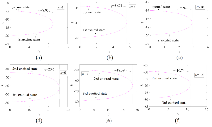
Figure 1: (Color online) Propagation constant $k$ vs. the gain-loss coefficient, $\gamma$, at fixed values $\varepsilon$, produced by a numerical solution of Eq. (27). Branches corresponding to the ground state, and the first, second, and third excited ones, are labeled accordingly.

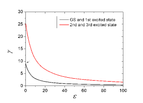
Figure 2: (Color online) Eigenvalues produced by the numerical solution of Eq. (27) for the GS (ground state) and first, second and third states remain real below the respective boundaries shown in the figure. For the GS and first state, the boundary starts from point $(\varepsilon,\gamma)=(0,8.95)$, as indicated by the black arrow.

IV Numerical results

IV.1 Symmetric and antisymmetric modes

Numerical solutions of nonlinear equations (2), (3) and (6), (7) were produced with the ideal $\delta$-function replaced by its regularized version,

$$\tilde{\delta}(x)=\frac{1}{\sqrt{\pi}\xi}\exp\left(-\frac{x^{2}}{\xi^{2}}\right),$$ (30)

with $\xi\ll 1$. Here, the results are presented for $\xi=0.05$ [taking smaller $\xi$ does not cause conspicuous differences in the results, except for Fig. 9(c), see below, where the agreement between the analytical and numerical stability boundaries improves if smaller $\xi$ is taken]. Solutions for the GS were generated by applying the imaginary-time method ITM1 -ITM3 to Eqs. (2) and (3). For producing the first excited state, to which the imaginary-time evolution cannot converge, the Newton’s iteration method was applied directly to Eqs. (6) and (7). The second excited state and higher-order ones could not be easily found by means of these algorithms. Stability of the stationary solutions was identified through calculation of the respective eigenvalue spectra, using Eq. (10), and then verified in direct simulations, by means of the Crank-Nicolson scheme.

Typical examples of stable $\mathcal{PT}$- symmetric and antisymmetric modes are displayed in Figs. 3(a,b). Unstable modes typically feature exponential growth of perturbations, leading blowup, as shown in Fig. 3(c). Additionally, in very narrow parameter regions (see Fig. 7 below), some antisymmetric modes exhibit weak oscillatory instability which transforms them into robust breathers via a supercritical bifurcation (cf. Ref. Barashenkov ), as shown in Fig. 3(d). This

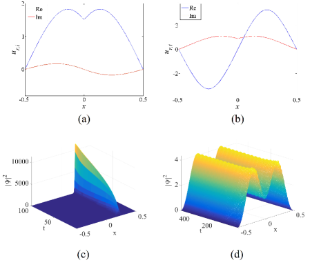
Figure 3: (Color online) Typical examples of a stable $\mathcal{PT}$-symmetric mode (a), and antisymmetric one (b), with parameters $(\varepsilon,\gamma,P,k)=(3,1,2,-7.2150)$ and $(\varepsilon,\gamma,P,k)=(3,3,6.05,-10)$, respectively. (c) The evolution of an unstable $\mathcal{PT}$-symmetric mode with $(\varepsilon,\gamma,P,k)=(3,1,5,-3.07)$. (d) The evolution of a weakly unstable $\mathcal{PT}$- antisymmetric mode with $(\varepsilon,\gamma,P,k)=(3,5.55,3.0202,-12)$.

We have also considered the model without the central barrier, by setting $\varepsilon=0$ in Eq. (2). In this case, it also produces $\mathcal{PT}$-symmetric and antisymmetric modes, typical examples of which are displayed in Figs. 4(a,b). However, if they are unstable, their instability, shown in Fig. 4(c,d), is different from what is shown above in Figs. 3(c,d). Namely, unstable $\mathcal{PT}$-symmetric modes transform into breathers, while the unstable $\mathcal{PT}$-antisymmetric ones transform from the excited state into the symmetric GS.

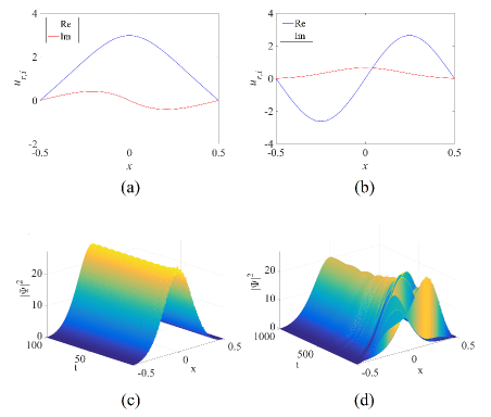
Figure 4: (Color online) The same as in Fig. 3, but for the system without the central barrier ($\varepsilon=0$). Typical examples of stable $\mathcal{PT}$-symmetric mode (a), and antisymmetric mode (b), for parameters $(\varepsilon,\gamma,P,k)=(0,3,4,1.0346)$ and $(\varepsilon,\gamma,P,k)=(0,3,3.5593,-14)$, respectively. (c) The evolution of an unstable $\mathcal{PT}$-symmetric mode with $(\varepsilon,\gamma,P,k)=(0,10,10,9.333)$. (d) The evolution of an unstable $\mathcal{PT}$-antisymmetric mode with $(\varepsilon,\gamma,P,k)=(0,3,8.71,-6)$.

IV.2 Existence and stability boundaries for families of the symmetric and antisymmetric modes

Families of $\mathcal{PT}$-symmetric and antisymmetric modes are characterized by relations between the propagation constant and total power, $k$ and $P$, which are presented in Fig. 5. It is worthy to note that they all satisfy the known necessary (but not sufficient) Vakhitov-Kolokolov stability criterion, $dP/dk>0$ VK1 -VK3 . We also notice that, for the GS (symmetric-mode) family, the stability segment shrinks with the increase of the gain-loss coefficient, $\gamma$. On the other hand, for the antisymmetric mode, the stability segments becomes shorter as one proceeds from $\gamma=0$ to $\gamma=1$, but this segment expands with the further increase of $\gamma$.

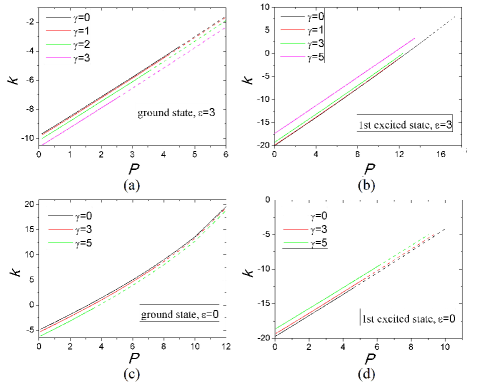
Figure 5: (Color online) Relations between the propagation constant, $k$, and the total power, $P$, for $\varepsilon=3$ and $0$, at different fixed values of the gain-loss coefficient, $\gamma$, for the $\mathcal{PT}$-symmetric mode (alias the ground state) (a,c) and the $\mathcal{PT}$-antisymmetric one (alias the first excited state) (b,d). Subfamilies of stable and unstable solutions are designated by continuous and dashed lines, respectively.

Results concerning the existence and stability of the symmetric and antisymmetric  states are summarized, severally, in parameter planes $(\gamma,P)$ and $(\varepsilon,P)$ displayed in Figs. 6 and 7. First, a salient feature of these results is that while, at $\varepsilon=0$, the antisymmetric mode has a smaller stability interval than its symmetric counterpart, its stability area at $\varepsilon>0$ is dramatically larger than the one for the symmetric mode. This difference is explained by the fact that the central barrier, imposed by $\varepsilon>0$, is favorable for the antisymmetric states, whose wave function nearly vanishes at $x=0$, and is obviously unfavorable for the symmetric states, which tend to have a maximum at $x=0$. Eventually, the antisymmetric states disappear at very larger values of $\varepsilon$, where the central potential barrier (30), multiplied by a very large $\varepsilon$, suppresses all possible modes in the potential box.

Furthermore, while a trend well-known in many $\mathcal{PT}$-symmetric systems is that the increase of the gain-loss coefficient, $\gamma$, leads to the breaking of the $\mathcal{PT}$ symmetry at a critical value of $\gamma$ bender1 -review2 , the stability region for the antisymmetric mode in Figs. 6(a,b) originally demonstrates slight expansion with the increase of $\gamma$, before the mode disappears at $\gamma$ exceeding the critical value. On the contrary, the symmetric mode features the usual trend to the destabilization, following the growth of $\gamma$, in Figs. 6(c,d).

Lastly, in the narrow top gray areas in Figs. 7(a,b,d), the antisymmetric mode is subject to the weak instability shown in Fig. 3(d), which does not destroy the mode, making it a weakly oscillating breather. On the other hand, in small gray regions at the bottom of Figs. 7(c,d), the antisymmetric mode is destroyed by the blowup instability.

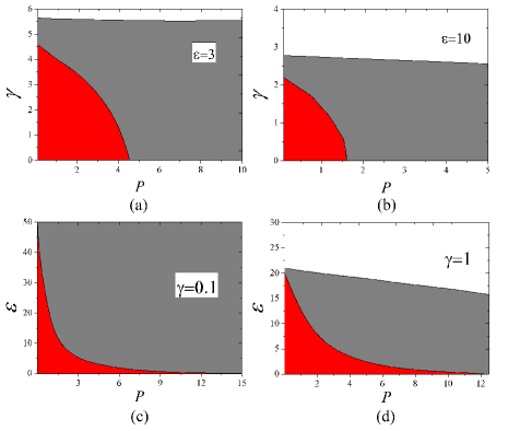
Figure 6: (Color online) Stability diagrams for the $\mathcal{PT}$-symmetric mode in plane $(\gamma,P)$ with fixed values of $\varepsilon=3$ (a) and $\varepsilon=10$ (b), and in plane $(\varepsilon,P)$, with fixed values of $\gamma=0.1$ (c) and $\gamma=1$ (d). Stable and unstable states exist in the red and gray areas, respectively. No solutions were found in white areas.

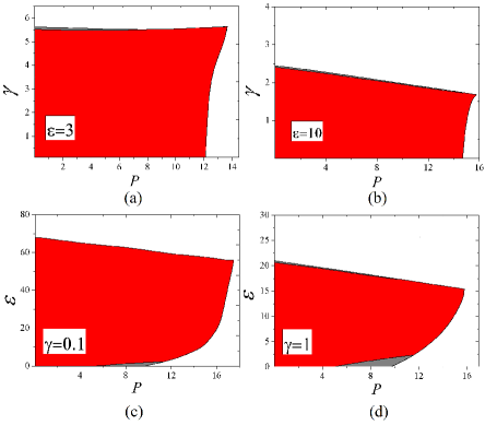
Figure 7: (Color online) The same as in Fig. 6, but for the $\mathcal{PT}$- antisymmetric mode. In the top narrow gray areas in panels (a), (b) and (d) the mode transforms into a weakly oscillating breather, as shown in Fig. 3(d), while unstable modes suffer blowup in small gray areas at the bottom of panels (c) and (d).

Stability diagrams for both symmetric and antisymmetric modes in the system without the splitting barrier (i.e., $\varepsilon=0$) are separately displayed in Fig. 8. Similar to what was noticed above, the stability region of $\mathcal{PT}$-symmetric mode shrinks with the increase of $\gamma$ for fixed $\varepsilon$, while, for the antisymmetric one, it initially expands, and then disappears at a critical value of $\gamma$. The unstable symmetric modes feature, respectively, both the transformation into a weakly oscillating breather [see Fig. 4(c)] and the blowup, below and above the dashed boundary in the gray area in Fig. 8(a).

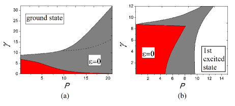
Figure 8: (Color online) Stability diagrams for $\mathcal{PT}$-symmetric (a) and antisymmetric (b) modes in the system without the box- splitting barrier ($\epsilon=0$). In panel (a), the gray area below the dashed boundary is populated by weakly unstable symmetric modes, which spontaneously transform into breathers, as shown in Fig. 4(c), while above the boundary the unstable models are destroyed by the blowup. In panel (b), the instability in the gray area leads to the spontaneous transformation of unstable $\mathcal{PT}$-antisymmetric modes into stable symmetric ones, as shown in Fig. 4(d).

The existence and stability diagrams produced for $\varepsilon=0$ must continuously extend to $\varepsilon\neq 0$. The continuity is illustrated by stability diagrams for the GS (symmetric state), plotted for small $\varepsilon$ in Fig. 9. In particular, panel (a) demonstrates that the gray area on the left-hand side of the dashed boundary, populated by the persistent breathers, shrinks with the increase of $\varepsilon$, and totally disappear at a small value, $\varepsilon\approx 0.27$. Panel (b) shows that the same area shrinks with the increase of $\gamma$, vanishing at $\gamma\approx 2.56$.

In all the cases, the increase of the total power, $P$, leads to destabilization of the modes, or to their eventual disappearance, as in the case displayed in Fig. 7. This trend is common for previously studied nonlinear $\mathcal{PT}$-symmetric systems bender1 -review2 .

Furthermore, Fig. 9(c) compares the prediction for the stability boundary of the $\mathcal{PT}$-symmetric mode, as given by the analytically derived equation (27), with the numerically found boundary, produced by the computation of the stability as per Eq. (10). For $\varepsilon\lesssim 10$, the analytical result well matches the numerical counterpart. At large values of $\varepsilon$, the agreement breaks down, the numerically identified stability region being much narrower than predicted analytically. The discrepancy is explained, as mentioned above in the different context, by the fact that the finite-width potential barrier (30), multiplied by large $\varepsilon$, strongly changes the model, in comparison with the underlying one which contains the ideal delta-function. The discrepancy decreases if smaller $\xi$ is used in Eq. (30), but, on the other hand, the use of the splitting barrier with a finite width corresponds to the physically realistic situation, as the infinitely narrow barrier cannot be implemented in the experiment.

Lastly, $\mathcal{PT}$-symmetric systems are characterized by the flux of power across the gain-loss interface, defined as

$$J=i\left(u_{x}u^{\ast}-u_{x}^{\ast}u\right)|_{x=0}.$$ (31)

Normally, $J$ is a growing function of the gain-loss coefficient, $\gamma$, but there are examples of systems demonstrating a jamming anomaly, with $dJ/d\gamma<0$. In the present model, typical examples of the $J(\gamma)$ dependence are displayed in Fig. 10. The dependences are practically linear (the linear form at small $\gamma$ can be easily explained by the perturbative analysis), without any trace of the jamming anomaly.

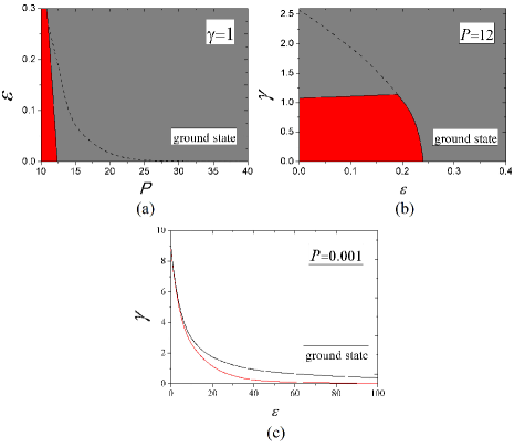
Figure 9: (Color online) Stability diagrams in the $(P,\varepsilon)$ plane with fixed $\gamma=1$ (a), and in the $(\varepsilon,\gamma)$ plane with fixed $P=12$ (b), for $\mathcal{PT}$-symmetric mode at small values of the barrier’s strength, $\varepsilon$. Regions of the weak oscillatory instability and blowup are located, severally, below and above dashed boundaries in (a) and (b). (c) The stability boundaries in the $(\varepsilon,\gamma)$ plane for the $\mathcal{PT}$- symmetric modes with a very small total power, $P=0.001$, which corresponds to the linearized system. Black and red curves represent the stability boundaries, as produced, respectively, by the analytical prediction [see Eq. (27)] and numerical results. The symmetric modes are stable beneath the respective boundaries.

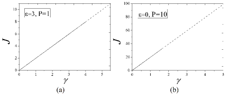
Figure 10: Power flux $J$ across the gain-loss interface, defined as per Eq. (31), versus the gain-loss coefficient, $\gamma$, for the cases of $\varepsilon=3$ (a), and $\varepsilon=0$ (b). In each panel, the total power, $P$, is fixed as indicated. The continuous and dashed segments represent stable and unstable solutions, respectively.

V Conclusion

The objective of this work is to introduce a basic one-dimensional $\mathcal{PT}$-symmetric model in the potential box, split into the double-well potential by the central $\delta$-functional barrier, with strength $\varepsilon$. The model includes constant linear gain and loss in two half-boxes, with strength $\gamma$, which lends the system the $\mathcal{PT}$ symmetry. The nonlinearity is represented by the usual cubic self-focusing. The system can be easily realized in guided microwaves and, in principle, in BEC too.

The stability of the zero state, which is a nontrivial problem for the present $\mathcal{PT}$-symmetric system, was investigated in the analytical form. Nonlinear $\mathcal{PT}$-symmetric and antisymmetric modes were found numerically, using, severally, the imaginary-time-integration and Newton-iteration methods, and replacing the ideal delta-functional barrier by a finite-width one. Their stability was explored through numerical computation of eigenvalues for small perturbations, and verified in direct simulations. In particular, the analytically predicted stability boundary for the zero state is confirmed by the numerical results, unless $\varepsilon$ is too large. The agreement breaks down at very large values of $\varepsilon$ because of the difference between the ideal delta-function and its regularized version used in the numerical calculations. Most of the unstable modes are destroyed by the blowup, which is typical for $\mathcal{PT}$-symmetric systems, but at small values of $\varepsilon$ the symmetric and antisymmetric modes spontaneously transform, respectively, into weakly oscillating breathers or stable symmetric GS (ground state). Unstable antisymmetric states also transform into weakly oscillating breathers in narrow regions near their existence boundary.

A noteworthy finding is that the stability region at $\varepsilon>0$ for the antisymmetric (first excited) state is much larger than for the symmetric GS, which is explained by the fact that the splitting potential favors antisymmetric configurations, and disfavors symmetric ones. The stability region of the symmetric states shrinks with the increase of $\gamma$ too, while for the the antisymmetric states it originally expands, but eventually disappears at a critical value of $\gamma$. As usual, the stability area of all the states shrinks with the increase of their total power.

A challenging possibility for the extension of the present work is to develop a two-dimensional counterpart of the model considered here.

Competing interests

The authors have no conflict of interests, in the context of this work.

Authors’ contributions

The model was designed by B.A.M., who was also responsible for the analytical part of the work. Numerical computations were carried out by Z.C. and Y.L., who also contributed to the analytical considerations. All the authors shared the responsibility for drafting the paper.

Funding

This work was supported, in part, by grant No. 1286/17 from the Israel Science Foundation, by grant No. 2015616 from the joint program in physics between NSF and Binational (US-Israel) Science Foundation, and by NNSFC (China) through Grant No. 11575063. Z.C. appreciates an excellence scholarship provided by the Tel Aviv University.

References

- (1) L. D. Landau and E. M. Lifshitz, Quantum Mechanics (Nauka Publishers: Moscow, 1974).
- (2) C. M. Bender and S. Boettcher, Real spectra in non-Hermitian Hamiltonians having symmetry. Phys. Rev. Lett. 80, 5243-5246 (1998).
- (3) P. Dorey, C. Dunning, and R. Tateo, Spectral equivalences, Bethe ansatz equations, and reality properties in -symmetric quantum mechanics, J. Phys. A: Math. Gen. 34, 5679-5704 (2001).
- (4) C. M. Bender, D. C. Brody, and H. F. Jones, Complex extension of quantum mechanics, Phys. Rev. Lett. 89, 270401 (2002).
- (5) C. M. Bender, Making sense of non-Hermitian Hamiltonians, Rep. Prog. Phys. 70, 947-1018 (2007).
- (6) C. M. Bender, Rigorous backbone of -symmetric quantum mechanics, J. Phys. A: Math. Theor. 49, 401002 (2016).
- (7) K. G. Makris, R. El-Ganainy, D. N. Christodoulides, and Z. H. Musslimani symmetric periodic optical potentials, Int. J. Theor. Phys. 50, 1019-1041 (2011).
- (8) N. Moiseyev, Non-Hermitian Quantum Mechanics, (Cambridge University Press, 2011).
- (9) L. Feng, R. El-Ganainy, and L. Ge, Non-Hermitian photonics based on parity-time symmetry, Nature Phot. 11, 752-762 (2017).
- (10) A. Ruschhaupt, F. Delgado, and J. G. Muga, Physical realization of -symmetric potential scattering in a planar slab waveguide, J. Phys. A: Math. Gen. 38, L171-L176 (2005).
- (11) R. El-Ganainy, K. G. Makris, D. N. Christodoulides, and Z. H. Musslimani, Theory of coupled optical -symmetric structures, Opt. Lett. 32, 2632-2634 (2007).
- (12) Z. H. Musslimani, K. G. Makris, R. El-Ganainy, and D. N. Christodoulides, Optical solitons in periodic potentials, Phys. Rev. Lett. 100, 030402 (2008).
- (13) M. V. Berry, Optical lattices with -symmetry are not transparent, J. Phys. A: Math. Theor. 41, 244007 (2008).
- (14) S. Klaiman, U. Günther, and N. Moiseyev, Visualization of branch points in -Symmetric Waveguides, Phys. Rev. Lett. 101, 080402 (2008).
- (15) S. Longhi, Bloch oscillations in complex crystals with symmetry, Phys. Rev. Lett. 103, 123601 (2009).
- (16) D. A. Zezyulin, Y. V. Kartashov, and V. V. Konotop, Stability of solitons in -symmetric nonlinear potentials, EPL 96, 64003 (2011).
- (17) R. Driben and B. A. Malomed, Stability of solitons in parity-time-symmetric couplers, Opt. Lett. 36, 4323-4325 (2011).
- (18) N. V. Alexeeva, I. V. Barashenkov, A. A. Sukhorukov, and Y. S. Kivshar, Optical solitons in -symmetric nonlinear couplers with gain and loss, Phys. Rev. A 85, 063837 (2012).
- (19) M.-A. Miri, A. B. Aceves, T. Kottos, V. Kovanis, and D. N. Christodoulides, Bragg solitons in nonlinear -symmetric periodic potentials, Phys. Rev. A 86, 033801 (2012).
- (20) S. Nixon, L. Ge, and J. Yang, Stability analysis for solitons in -symmetric optical lattices, Phys. Rev. A 85, 023822 (2012).
- (21) J. Yang, Symmetry breaking of solitons in one-dimensional parity-time-symmetric optical potentials, Opt. Lett. 39, 5547-5550 (2014).
- (22) Y. V. Kartashov, B. A. Malomed, and L. Torner, Unbreakable symmetry of solitons supported by inhomogeneous defocusing nonlinearity, Opt. Lett. 39, 5641-5644 (2014).
- (23) Z. Chen, J. Liu, S. Fu, Y. Li, and B. A. Malomed, Discrete solitons and vortices on two-dimensional lattices of -symmetric couplers, Opt. Express 22, 29679(2014).
- (24) Y. Kominis, T. Bountis, and S. Flach, Stability through asymmetry: Modulationally stable nonlinear supermodes of asymmetric non-Hermitian optical couplers, Phys. Rev. 95, 063832 (2017).
- (25) P. Glansdorff and I. Prigogine, Thermodynamic Theory of Structures, Stability and Fluctuations (John Wiley & Sons: New York, 1971).
- (26) A. Guo, G. J. Salamo, D. Duchesne, R. Morandotti, M. Volatier-Ravat, V. Aimez, G. A. Siviloglou, and D.. N. Christodoulides, Observation of -symmetry breaking in complex optical potentials, Phys. Rev. Lett. 103, 093902 (2009).
- (27) C. E. Rüter, K. G. Makris, R. El-Ganainy, D. N. Christodoulides, M. Segev, and D. Kip, Observation of parity-time symmetry in optics. Nature Phys. 6, 192-195 (2010).
- (28) A. Regensburger, C. Bersch, M. A. Miri, G. Onishchukov, D. N. Christodoulides, and U. Peschel, Parity-time synthetic photonic lattices, Nature 488, 167-171 (2012).
- (29) M. Wimmer, A. Regensburger, M. A. Miri, C. Bersch, D. N. Christodoulides, and U. Peschel, Observation of optical solitons in -symmetric lattices, Nature Commun. 6, 7782 (2015).
- (30) H. Hodaei, M. A. Miri, M. Heinrich, D. N. Christodoulides, and M. Khajavikhan, Parity-time-symmetric microring lasers, Science 346, 975-978 (2014).
- (31) S. Longhi, -symmetric laser absorber, Phys. Rev. A 82, 031801 (2010).
- (32) G. Castaldi, S. Savoia, V. Galdi, A. Alù, A. and N. Engheta, metamaterials via complex-coordinate transformation optics, Phys. Rev. Lett. 110, 173901 (2013).
- (33) B. Peng, Ş. K. Özdemir, W. Chen, F. Nori, and L. Yang, Parity-time-symmetric whispering gallery microcavities, Nature Phys. 10, 394-398 (2014).
- (34) Z. Zhang, Y. Zhang, J. Sheng, L. Yang, M. A. Miri, D. N. Christodoulides, B. He, Y. Zhang, and M. Xiao, Observation of parity-time symmetry in optically induced atomic lattices, Phys. Rev. Lett. 117, 123601 (2016).
- (35) J.-Y. Lien, Y.-N. Chen, N. Ishida, H.-B. Chen, C.-C. Hwang, and F. Nori, Multistability and condensation of exciton-polaritons below threshold, Phys. Rev. B 91, 024511 (2015).
- (36) T. Gao,E. Estrecho, K. Y. Bliokh, T. C. H. Liew, M. D. Fraser, S. Brodbeck, M. Kamp, C. Schneider, S. Höfling, Y. Yamamoto, F. Nori, Y. S. Kivshar, A. G. Truscott, R. G. Dall, and E. A. Ostrovskaya, Observation of non-Hermitian degeneracies in a chaotic exciton-polariton billiard, Nature 526, 554-558 (2015).
- (37) I. Yu. Chestnov, S. S. Demirchyan, A. P. Alodjants, Y. G. Rubo, and A. V. Kavokin, Permanent Rabi oscillations in coupled exciton-photon systems with -symmetry, Sci. Rep. 6, 19551 (2016).
- (38) X. Zhu, H. Ramezani, C. Shi, J. Zhu, and X. Zhang, -Symmetric Acoustics, Phys. Rev. X 4 031042 (2014).
- (39) R. Fleury, D. Sounas, and A. Alú, An invisible acoustic sensor based on parity-time symmetry, Nature Communications 6, 5905 (2015).
- (40) X.-W. Xu, Y.-x. Liu, C.-P. Sun, and Y. Li, Mechanical symmetry in coupled optomechanical systems, Phys. Rev. A 92 013852 (2015).
- (41) J. Schindler, Z. Lin, J. M. Lee, H. Ramezani, F. M. Ellis, and T. Kottos, J. Phys. A: Math. Theor. 45, 444029 (2012).
- (42) L. Schwarz, H. Cartarius, Z. H. Musslimani, J. Main, and G. Wunner, Vortices in Bose-Einstein condensates with -symmetric gain and loss, Phys. Rev. 95, 053613 (2017).
- (43) J. M. Lee, T. Kottos, and B. Shapiro, Macroscopic magnetic structures with balanced gain and loss, Phys. Rev. B 91, 094416 (2015).
- (44) C. M. Bender, D. C. Brody, and J.-H. Chen, -symmetric extension of the Korteweg-de Vries equation, J. Phys. A: Math. Theor. 40, F153-F160 (2007).
- (45) A. Fring, -symmetric deformations of the Korteweg-de Vries equation, J. Phys. A: Math. Theor. 40, 4215-4334 (2007).
- (46) Z. Y. Yan, Complex -symmetric nonlinear Schrödinger equation and Burgers equation, Phil. Trans. Roy. Soc. A - Math Phys. Eng. Sci. 371, 20120059 (2013).
- (47) J. Cuevas-Maraver, B. Malomed, and P. Kevrekidis, A -symmetric dual-core system with the sine-Gordon nonlinearity and derivative coupling, Symmetry 8, 39 (2016).
- (48) H. Sakaguchi and B. A. Malomed, One- and two-dimensional solitons in -symmetric systems emulating spin-orbit coupling, New J. Phys. 18, 105005 (2016).
- (49) V. V. Konotop, J. Yang, and D. A. Zezyulin, Nonlinear waves in -symmetric systems, Rev. Mod. Phys. 88, 035002 (2016).
- (50) S. V. Suchkov, A. A. Sukhorukov, J. H. Huang, S. V. Dmitriev, C. Lee, and Y. S. Kivshar, Nonlinear switching and solitons in -symmetric photonic systems, Laser and Photonics Reviews 10, 177-213 (2016).
- (51) J. Yang, Necessity of symmetry for soliton families in one-dimensional complex potentials, Phys. Lett. A, 378, 367-373 (2014).
- (52) B. A. Malomed, Evolution of nonsoliton and “quasiclassical” wavetrains in nonlinear Schrödinger and Korteweg - de Vries equations with dissipative perturbations, Physica D 29, 155-172 (1987).
- (53) E. V. Vanin, A. I. Korytin, A. M. Sergeev, D. Anderson, M. Lisak, and L. Vázquez, Dissipative optical solitons, Phys. Rev. A 49, 2806-2811 (1994).
- (54) E. N. Tsoy, A. Ankiewicz, and N. Akhmediev, Dynamical models for dissipative localized waves of the complex Ginzburg-Landau equation, Phys. Rev. E 73, 036621 (2006).
- (55) M. L. Chiofalo, S. Succi, and M. P. Tosi, Ground state of trapped interacting Bose-Einstein condensates by an explicit imaginary-time algorithm, Phys. Rev. E 62, 7438-7444 (2000).
- (56) W. Bao and Q. Du, Computing the ground state solution of Bose-Einstein condensates by a normalized gradient flow, SIAM J. Sci. Comput. 25, 1674-1697 (2004).
- (57) X. Antoine, W. Bao, and C. Besse, Computational methods for the dynamics of the nonlinear Schrödinger/Gross–Pitaevskii equations, Comp. Phys. Commun. 184, 2621-2633 (2013).
- (58) M. Vakhitov and A. Kolokolov, Stationary solutions of the wave equation in a medium with nonlinearity saturation, Radiophys. Quantum Electron. 16, 783 (1973).
- (59) L. Bergé, Wave collapse in physics: Principles and applications to light and plasma waves, Phys. Rep. 303, 259 (1998).
- (60) G. Fibich, The Nonlinear Schrödinger Equation: Singular Solutions and Optical Collapse (Springer, Cham, 2015).
- (61) G. J. Milburn, J. Corney, E. M. Wright, and D. F. Walls, Quantum dynamics of an atomic Bose-Einstein condensate in a double-well potential, Phys. Rev. A 55, 4318 (1997).
- (62) A. Smerzi, S. Fantoni, S. Giovanazzi, and S. R. Shenoy, Quantum coherent atomic tunneling between two trapped Bose-Einstein condensates, Phys. Rev. Lett. 79, 4950 (1997).
- (63) M. Albiez, R. Gati, J. Fölling, S. Hunsmann, M. Cristiani, and M. K. Oberthaler, Direct observation of tunneling and nonlinear self-trapping in a single bosonic Josephson junction, Phys. Rev. Lett. 95, 010402 (2005).
- (64) I. V. Barashenkov and D. A. Zezyulin, Localised nonlinear modes in the -symmetric double-delta well Gross-Pitaevskii equation, in: Non-Hermitian Hamiltonians in Quantum Physics, Selected Contributions from the 15th International Conference on Non-Hermitian Hamiltonians in Quantum Physics (Palermo, Italy, 18-23 May 2015), pp. 123-142. Editors: F. Bagarello, R. Passante, and Ca. Trapani.
- (65) K. B. Zegadlo, N. Dror, M. Trippenbach, M. A. Karpierz, and B. A. Malomed, Spontaneous symmetry breaking of self-trapped and leaky modes in quasi-double-well potentials, Phys. Rev. A 93, 023644 (2016).
- (66) B. A. Malomed, editor, Spontaneous Symmetry Breaking, Self-Trapping, and Josephson Oscillations (Springer: Berlin, 2013).
- (67) B. A. Malomed, Symmetry breaking in laser cavities, Nature Photon. 9, 287 (2015).
- (68) E. Shamriz, N. Dror, and B. A. Malomed, Spontaneous symmetry breaking in a split potential box, Phys. Rev. E 94, 022211 (2016).
- (69) D. Deslandes and K. Wu, Integrated microstrip and rectangular waveguide in planar form, IEEE Microwave Wireless Comp. Lett. 11, 68-70 (2001).
- (70) A. Slavin and V. Tiberkevich, Nonlinear auto-oscillator theory of microwave generation by spin-polarized current, IEEE Trans. Magnetics 45, 1875-1918 (2009).
- (71) I. V. Barashenkov, S. V. Suchkov, A. A. Sukhorukov, S. V. Dmitriev and Y. Kivshar, Breathers in -symmetric optical couplers, Phys. Rev. A 86, 053809 (2012).
- (72) I. V. Barashenkov, D. A. Zezyulin and V. V. Konotop, Jamming anomaly in -symmetric systems, New J. Phys. 18, 075015 (2016).