Generation Of Complete Test Sets

Abstract

We use testing to check if a combinational circuit $N$ always evaluates to 0 (written as $N\equiv 0$). The usual point of view is that to prove $N\equiv 0$ one has to check the value of $N$ for all $2^{|X|}$ input assignments where $X$ is the set of input variables of $N$. We use the notion of a Stable Set of Assignments (SSA) to show that one can build a complete test set (i.e. a test set proving $N\equiv 0$) that consists of less than $2^{|X|}$ tests. Given an unsatisfiable CNF formula $H(W)$, an SSA of $H$ is a set of assignments to $W$ proving unsatisfiability of $H$. A trivial SSA is the set of all $2^{|W|}$ assignments to $W$. Importantly, real-life formulas can have SSAs that are much smaller than $2^{|W|}$. Generating a complete test set for $N$ using only the machinery of SSAs is inefficient. We describe a much faster algorithm that combines computation of SSAs with resolution derivation and produces a complete test set for a “projection” of $N$ on a subset of variables of $N$. We give experimental results and describe potential applications of this algorithm.

1 Introduction

Testing is an important part of verification flows. For that reason, any progress in understanding testing and improving its quality is of great importance. In this paper, we consider the following problem. Given a single-output combinational circuit $N$, find a set of input assignments (tests) proving that $N$ evaluates to 0 for every test (written as $N\equiv 0$) or find a counterexample. We will call a set of input assignments proving $N\equiv 0$ a complete test set (CTS). We will call a CTS trivial if it consists of all possible tests. Typically, one assumes that proving $N\equiv 0$ involves derivation of a trivial CTS, which is infeasible in practice. Thus, testing is used only for finding an input assignment refuting $N\equiv 0$. In this paper, we present an approach for building a non-trivial CTS that consists only of a subset of all possible tests.

Let $N(X,Y,z)$ be a single-output combinational circuit where $X$ and $Y$ are sets of variables specifying input and internal variables of $N$ respectively. Variable $z$ specifies the output of $N$. Let $F_{N}(X,Y,z)$ be a formula defining the functionality of $N$ (see Section 3). We will denote the set of variables of circuit $N$ (respectively formula $H$) as $\mathit{Vars}(N)$ (respectively $\mathit{Vars}(H)$). Every assignment to $\mathit{Vars}(F_{N})$ satisfying $F_{N}$ corresponds to a consistent assignment to $\mathit{Vars}(N)$ and vice versa. Then the problem of proving $N\equiv 0$ reduces to showing that formula $F_{N}\wedge z$ is unsatisfiable. From now on, we assume that all formulas mentioned in this paper are propositional. Besides, we will assume that every formula is represented in CNF i.e. as a conjunction of disjunctions of literals. We will also refer to a disjunction of literals as a clause.

Our approach is based on the notion of a Stable Set of Assignments (SSA) introduced in [10]. Given formula $H(W)$, an SSA of $H$ is a set $P$ of assignments to variables of $W$ that have two properties. First, every assignment of $P$ falsifies $H$. Second, $P$ is a transitive closure of some neighborhood relation between assignments (see Section 2). The fact that $H$ has an SSA means that the former is unsatisfiable. Otherwise, an assignment satisfying $H$ is generated when building its SSA. If $H$ is unsatisfiable, the set of all $2^{|W|}$ assignments is always an SSA of $H$ . We will refer to it as trivial. Importantly, a real-life formula $H$ can have a lot of SSAs whose size is much less than $2^{|W|}$. We will refer to them as non-trivial. As we show in Section 2, the fact that $P$ is an SSA of $H$ is a structural property of the latter. That is this property cannot be expressed in terms of the truth table of $H$ (as opposed to a semantic property of $H$). For that reason, if $P$ is an SSA for $H$, it may not be an SSA for some other formula $H^{\prime}$ that is logically equivalent to $H$.

We show that a CTS for $N$ can be easily extracted from an SSA of formula $F_{N}\wedge z$. This makes a non-trivial CTS a structural property of circuit $N$ that cannot be expressed in terms of its truth table. Unfortunately, building an SSA even for a formula of small size is inefficient. To address this problem, we present a procedure that constructs a simpler formula $H(V)$ where $V\subseteq\mbox{$\mathit{Vars}(F_{N}\wedge z)$}$ for which an SSA is generated. Formula $H$ is implied by $F_{N}\wedge z$. Thus, the unsatisfiability of $H$ proved by construction of its SSA implies that $F_{N}\wedge z$ is unsatisfiable too and $N\equiv 0$. A test set extracted from an SSA of $H$ can be viewed as a CTS for a “projection” of $N$ on variables of $V$.

We will refer to the procedure for building formula $H$ above as $\mathit{SemStr}$ (“Semantics and Structure”). The name is due to the fact that $\mathit{SemStr}$ combines semantic and structural derivations. $\mathit{SemStr}$ can be applied to an arbitrary CNF formula $G(V,W)$. If $G$ is unsatisfiable, $\mathit{SemStr}$ returns a formula $H(V)$ implied by $G$ and its SSA. Otherwise, it produces an assignment to $V\cup W$ satisfying $G$. The semantic part of $\mathit{SemStr}$ is to derive $H$. Its structural part consists of proving that $H$ is unsatisfiable by constructing an SSA. Formula $H$ produced when $G$ is unsatisfiable is logically equivalent to $\exists{W}[G]$. Thus, $\mathit{SemStr}$ can be viewed as a quantifier elimination algorithm for unsatisfiable formulas. On the other hand, $\mathit{SemStr}$ can be applied to check satisfiability of a CNF formula, which makes it a SAT-algorithm.

The notion of non-trivial CTSs helps better understand testing. The latter is usually considered as an incomplete version of a semantic derivation. This point of view explains why testing is efficient (because it is incomplete) but does not explain why it is effective (only a minuscule part of the truth table is sampled). Since a non-trivial CTS for $N$ is its structural property, it is more appropriate to consider testing as a version of a structural derivation (possibly incomplete). This point of view explains not only efficiency of testing but provides a better explanation for its effectiveness: by using circuit-specific tests one can cover a significant part of a non-trivial CTS.

The contribution of this paper is threefold. First, we use the machinery of SSAs to introduce the notion of non-trivial CTSs (Section 3). Second, we present $\mathit{SemStr}$, a SAT-algorithm that combines structural and semantic derivations (Section 4). We show that this algorithm can be used for computing a CTS for a projection of a circuit. We also discuss some applications of $\mathit{SemStr}$ (Sections 6 and 7). Third, we give experimental results showing the effectiveness of tests produced by $\mathit{SemStr}$ (Section 8). In particular, we describe a procedure for “piecewise” construction of test sets that can be potentially applied to very large circuits.

2 Stable Set Of Assignments

2.1 Some definitions

Let $\vec{p}$ be an assignment to a set of variables $V$. Let $\vec{p}$ falsify a clause $C$. Denote by $\mathit{Nbhd}({\mbox{$\vec{p}$}},C)$ the set of assignments to $V$ satisfying $C$ that are at Hamming distance 1 from $\vec{p}$. (Here Nbhd stands for “Neighborhood”). Thus, the number of assignments in $\mathit{Nbhd}({\mbox{$\vec{p}$}},C)$ is equal to that of literals in $C$. Let $\vec{q}$ be another assignment to $V$ (that may be equal to $\vec{p}$). Denote by $\mathit{Nbhd}({\mbox{$\vec{q}$}},{\mbox{$\vec{p}$}},C)$ the subset of $\mathit{Nbhd}({\mbox{$\vec{p}$}},C)$ consisting only of assignments that are farther away from $\vec{q}$ than $\vec{p}$ (in terms of the Hamming distance).

Example 1

Let $V=\mbox{$\{v_{1},v_{2},v_{3},v_{4}\}$}$ and $\vec{p}$=0110. We assume that the values are listed in $\vec{p}$ in the order the corresponding variables are numbered i.e. $v_{1}=0$, $v_{2}=1,v_{3}=1,v_{4}=0$. Let $C=v_{1}\vee\overline{v_{3}}$. (Note that $\vec{p}$ falsifies $C$.) Then $\mathit{Nbhd}({\mbox{$\vec{p}$}},C)$=$\{{\mbox{$\vec{p}_{1}$}},{\mbox{$\vec{p}_{2}$}}\}$ where $\vec{p}_{1}$ = 1110 and $\vec{p}_{2}$=0100. Let $\vec{q}$ = 0000. Note that $\vec{p}_{2}$ is actually closer to $\vec{q}$ than $\vec{p}$. So $\mathit{Nbhd}({\mbox{$\vec{q}$}},{\mbox{$\vec{p}$}},C)$=$\{{\mbox{$\vec{p}_{1}$}}\}$.

Definition 1

Let $H$ be a formula specified by a set of clauses $\{C_{1},\dots,C_{k}\}$. Let $P$ = $\{{\mbox{$\vec{p}_{1}$}},\dots,{\mbox{$\vec{p}_{m}$}}\}$ be a set of assignments to $\mathit{Vars}(H)$ such that every ${\mbox{$\vec{p}_{i}$}}\in P$ falsifies $H$. Let $\Phi$ denote a mapping $P\rightarrow H$ where $\Phi({\mbox{$\vec{p}_{i}$}})$ is a clause $C$ of $H$ falsified by $\vec{p}_{i}$. We will call $\Phi$ an AC-mapping where “AC” stands for “Assignment-to-Clause”. We will denote the range of $\Phi$ as $\Phi(P)$. (So, a clause $C$ of $H$ is in $\Phi(P)$ iff there is an assignment ${\mbox{$\vec{p}_{i}$}}\in P$ such that $C=\mbox{$\Phi$}({\mbox{$\vec{p}_{i}$}})$.)

Definition 2

Let $H$ be a formula specified by a set of clauses $\{C_{1},\dots,C_{k}\}$. Let $P$ = $\{{\mbox{$\vec{p}_{1}$}},\dots,{\mbox{$\vec{p}_{m}$}}\}$ be a set of assignments to $\mathit{Vars}(H)$. $P$ is called a Stable Set of Assignments (SSA) of $H$ with center $\mbox{$\vec{p}_{\mathit{init}}$}\in P$ if there is an AC-mapping $\Phi$ such that for every ${\mbox{$\vec{p}_{i}$}}\in P$, $\mbox{$\mathit{Nbhd}(\mbox{$\vec{p}_{\mathit{init}}$},{\mbox{$\vec{p}_{i}$}},C)$}\subseteq P$ holds where $C=\mbox{$\Phi({\mbox{$\vec{p}_{i}$}})$}$.

Note that if $P$ is an SSA of $H$ with respect to AC-mapping $\Phi$, then $P$ is also an SSA of $\Phi(P)$.

Example 2

Let $H$ consist of four clauses: $C_{1}=v_{1}\vee v_{2}\vee v_{3}$, $C_{2}=\overline{v}_{1}$, $C_{3}=\overline{v}_{2}$, $C_{4}=\overline{v}_{3}$. Let $P=\mbox{$\{{\mbox{$\vec{p}_{1}$}},{\mbox{$\vec{p}_{2}$}},{\mbox{$\vec{p}_{3}$}},{\mbox{$\vec{p}_{4}$}}\}$}$ where ${\mbox{$\vec{p}_{1}$}}=000$, ${\mbox{$\vec{p}_{2}$}}=100$, ${\mbox{$\vec{p}_{3}$}}=010$, ${\mbox{$\vec{p}_{4}$}}=001$. Let $\Phi$ be an AC-mapping specified as $\mbox{$\Phi({\mbox{$\vec{p}_{i}$}})$}=C_{i},i=1,\dots,4$. Since $\vec{p}_{i}$ falsifies $C_{i}$, $i=1,\dots,4$,  $\Phi$ is a correct AC-mapping. Set $P$ is an SSA of $H$ with respect to $\Phi$ and center $\vec{p}_{\mathit{init}}$=$\vec{p}_{1}$. Indeed, $\mathit{Nbhd}(\mbox{$\vec{p}_{\mathit{init}}$},{\mbox{$\vec{p}_{1}$}},C_{1})$=$\{{\mbox{$\vec{p}_{2}$}},{\mbox{$\vec{p}_{3}$}},{\mbox{$\vec{p}_{4}$}}\}$ where $C_{1}=\mbox{$\Phi({\mbox{$\vec{p}_{1}$}})$}$ and $\mathit{Nbhd}(\mbox{$\vec{p}_{\mathit{init}}$},{\mbox{$\vec{p}_{i}$}},C_{i})$ = $\emptyset$, where $C_{i}=\mbox{$\Phi({\mbox{$\vec{p}_{i}$}})$}$, $i=2,3,4$. Thus, $\mathit{Nbhd}(\mbox{$\vec{p}_{\mathit{init}}$},{\mbox{$\vec{p}_{i}$}},\mbox{$\Phi({\mbox{$\vec{p}_{i}$}})$})\subseteq P$, $i=1,\dots,4$.

2.2 SSAs and satisfiability of a formula

Proposition 1

Formula $H$ is unsatisfiable iff it has an SSA.

The proof is given in Section 0.A of the appendix. A similar proposition was proved in [10] for “uncentered” SSAs (see Footnote 6).

Corollary 1

Let $P$ be an SSA of $H$ with respect to PC-mapping $\Phi$. Then the set of clauses $\Phi(P)$ is unsatisfiable. Thus, every clause of $H\setminus\mbox{$\Phi(P)$}$ is redundant.

The set of all assignments to $\mathit{Vars}(H)$ forms the trivial uncentered SSA of $H$. Example 2 shows a non-trivial SSA. The fact that formula $H$ has a non-trivial SSA $P$ is its structural property. That is one cannot express the fact that $P$ is an SSA of $H$ using only the truth table of $H$. For that reason, $P$ may not be an SSA of a formula $H^{\prime}$ logically equivalent to $H$.

$\mathit{BuildPath}(H,\mbox{$\Phi$},\mbox{$\vec{p}_{\mathit{init}}$},\vec{s})${
1	$\mathit{Path}:=\mathit{nil}$
2	$\vec{p}_{1}:=\mbox{$\vec{p}_{\mathit{init}}$}$
3	$i:=1$
4	while ($\vec{p}_{i}\neq\vec{s}$) {
5		$\mathit{Path}:=\mathit{AddAssgn}(\mathit{Path},\vec{p}_{i})$
6		$C:=\mbox{$\Phi({\mbox{$\vec{p}_{i}$}})$}$
7*		$v:=\mathit{FindVar}(C,\vec{p}_{i},\vec{s})$
8		$\vec{p}_{i+1}:=\mathit{FlipVar}(\vec{p}_{i},v)$
9		$i:=i+1$ }
10	return($\mathit{Path}$) }

Figure 1: BuildPath procedure

The relation between SSAs and satisfiability can be explained as follows. Suppose that formula $H$ is satisfiable. Let $\vec{p}_{\mathit{init}}$ be an arbitrary assignment to $\mathit{Vars}(H)$ and $\vec{s}$ be a satisfying assignment that is the closest to $\vec{p}_{\mathit{init}}$ in terms of the Hamming distance. Let $P$ be the set of all assignments to $\mathit{Vars}(H)$ that falsify $H$ and $\Phi$ be an AC-mapping from $P$ to $H$. Then $\vec{s}$ can be reached from $\vec{p}_{\mathit{init}}$ by procedure BuildPath shown in Figure 1. (This procedure is non-deterministic: an oracle is used in line 7 to pick a variable to flip.) It generates a sequence of assignments ${\mbox{$\vec{p}_{1}$}},\dots,{\mbox{$\vec{p}_{i}$}}$ where $\vec{p}_{1}$ = $\vec{p}_{\mathit{init}}$ and $\vec{p}_{i}$=$\vec{s}$. First, BuildPath checks if current assignment $\vec{p}_{i}$ equals $\vec{s}$. If so, then $\vec{s}$ has been reached. Otherwise, BuildPath uses clause $C=\mbox{$\Phi({\mbox{$\vec{p}_{i}$}})$}$ to generate next assignment. Since $\vec{s}$ satisfies $C$, there is a variable $v\in\mbox{$\mathit{Vars}(C)$}$ that is assigned differently in $\vec{p}_{i}$ and $\vec{s}$. BuildPath generates a new assignment $\vec{p}_{i+1}$ obtained from $\vec{p}_{i}$ by flipping the value of $v$.

BuildPath converges to $\vec{s}$ in $k$ steps where $k$ is the Hamming distance between $\vec{p}$ and $\vec{s}$. Importantly, BuildPath reaches $\vec{s}$ for any AC-mapping. Let $P$ be an SSA of $H$ with respect to center $\vec{p}_{\mathit{init}}$ and AC-mapping $\Phi$. Then if BuildPath starts with $\vec{p}_{\mathit{init}}$ and uses $\Phi$ as AC-mapping, it can reach only assignments of $P$. Since every assignment of $P$ falsifies $H$, no satisfying assignment can be reached.

$\mathit{BuildSSA}(H)${
1	$E=\emptyset$; $\mbox{$\Phi$}:=\emptyset$
2	$\mbox{$\vec{p}_{\mathit{init}}$}:=\mathit{PickInitAssgn}(H)$
3	$Q:=\mbox{$\{\mbox{$\vec{p}_{\mathit{init}}$}\}$}$
4	while ($Q\neq\emptyset$) {
5		${\mbox{$\vec{p}$}}:=\mathit{PickAssgn}(\mathit{Q})$
6		$\mathit{Q}:=\mathit{Q}\setminus\mbox{$\{{\mbox{$\vec{p}$}}\}$}$
7		if $(\mathit{SatAssgn}({\mbox{$\vec{p}$}},H))$
8			return(${\mbox{$\vec{p}$}},\mathit{nil},\mathit{nil},\mathit{nil}$)
9		$C:=\mathit{PickFalsifClause}(H,{\mbox{$\vec{p}$}})$
10		$New:=\mbox{$\mathit{Nbhd}(\mbox{$\vec{p}_{\mathit{init}}$},{\mbox{$\vec{p}$}},C)$}\setminus E$
11		$Q:=Q\cup New$
12		$E:=E\cup\mbox{$\{{\mbox{$\vec{p}$}}\}$}$
13		$\mbox{$\Phi$}:=\mbox{$\Phi$}\cup\mbox{$\{({\mbox{$\vec{p}$}},C)\}$}$}
14	return($\mathit{nil},E,\mbox{$\vec{p}_{\mathit{init}}$},\mbox{$\Phi$}$) }

Figure 2: BuildSSA procedure

A procedure for generation of SSAs called BuildSSA is shown in Figure 2. It accepts formula $H$ and outputs either a satisfying assignment or an SSA of $H$, a center $\vec{p}_{\mathit{init}}$ and AC-mapping $\Phi$. BuildSSA maintains two sets of assignments denoted as $E$ and $Q$. Set $E$ contains the examined assignments i.e. ones whose neighborhood is already explored. Set $Q$ specifies assignments that are queued to be examined. $Q$ is initialized with an assignment $\vec{p}_{\mathit{init}}$ and $E$ is originally empty. BuildSSA updates $E$ and $Q$ in a while loop. First, BuildSSA picks an assignment $\vec{p}$ of $Q$ and checks if it satisfies $H$. If so, $\vec{p}$ is returned as a satisfying assignment. Otherwise, BuildSSA removes $\vec{p}$  from $Q$ and picks a clause $C$ of $H$ falsified by $\vec{p}$. The assignments of $\mathit{Nbhd}(\mbox{$\vec{p}_{\mathit{init}}$},{\mbox{$\vec{p}$}},C)$ that are not in $E$ are added to $Q$. After that, $\vec{p}$ is added to $E$ as an examined assignment, pair $({\mbox{$\vec{p}$}},C)$ is added to $\Phi$ and a new iteration begins. If $Q$ is empty, $E$ is an SSA with center $\vec{p}_{\mathit{init}}$ and AC-mapping $\Phi$.

3 Complete Test Sets

Let $N(X,Y,z)$ be a single-output combinational circuit where $X$ and $Y$ are sets of variables specifying input and internal variables of $N$. Variable $z$ specifies the output of $N$. Let $N$ consist of gates $G_{1},\dots,G_{k}$. Then $N$ can be represented as CNF formula $F_{N}=F_{G_{1}}\wedge\dots\wedge F_{G_{k}}$ where $F_{G_{i}},i=1,\dots,k$ is a CNF formula specifying the consistent assignments of gate $G_{i}$. Proving $N\equiv 0$ reduces to showing that formula $F_{N}\wedge z$ is unsatisfiable.

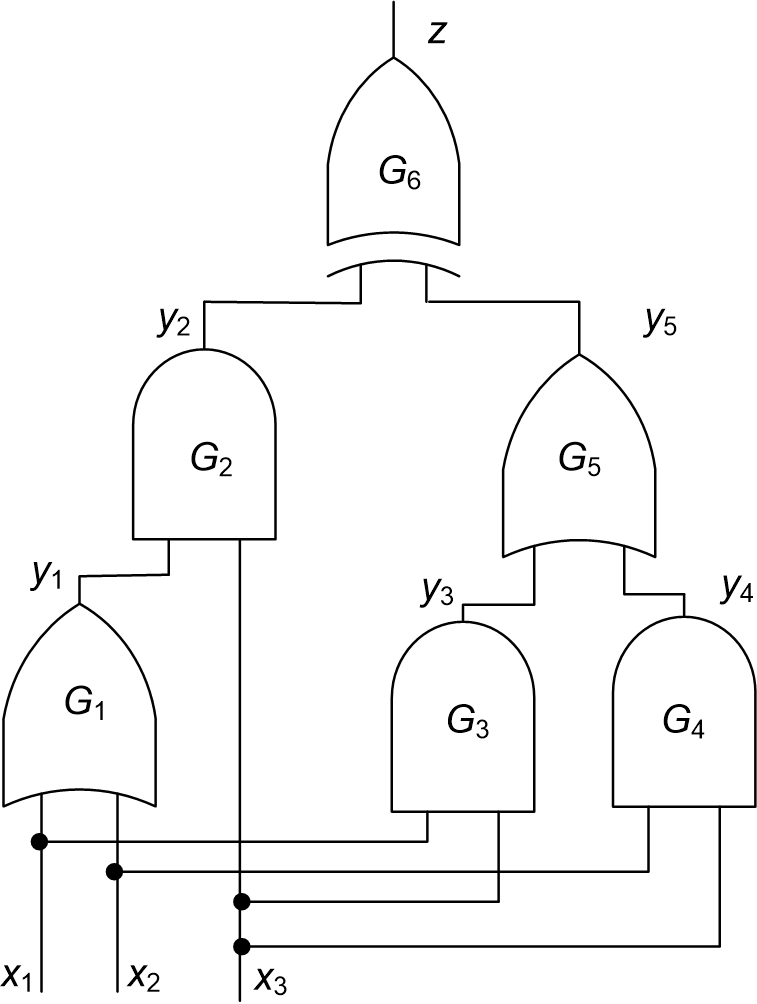
Figure 3: Example of circuit $N(X,Y,z)$

Example 3

Circuit $N$ shown in Figure 3 represents equivalence checking of expressions $(x_{1}\vee x_{2})\wedge x_{3}$ and $(x_{1}\wedge x_{3})\vee(x_{2}\wedge x_{3})$. The former is specified by gates $G_{1}$ and $G_{2}$ and the latter by $G_{3}$, $G_{4}$ and $G_{5}$. Formula $F_{N}$ is equal to $F_{G_{1}}\wedge\dots\wedge F_{G_{6}}$ where, for instance, $F_{G_{1}}=C_{1}\wedge C_{2}\wedge C_{3}$, $C_{1}=x_{1}\vee x_{2}\vee\overline{y}_{1}$, $C_{2}=\overline{x}_{1}\vee y_{1}$, $C_{3}=\overline{x}_{2}\vee y_{1}$. Every satisfying assignment to $\mathit{Vars}(F_{G_{1}})$ corresponds to a consistent assignment to gate $G_{1}$ and vice versa. For instance, $(x_{1}=0,x_{2}=0,y_{1}=0)$ satisfies $F_{G_{1}}$ and is a consistent assignment to $G_{1}$ since the latter is an OR gate. Formula $F_{N}\wedge z$ is unsatisfiable due to functional equivalence of expressions $(x_{1}\vee x_{2})\wedge x_{3}$ and $(x_{1}\wedge x_{3})\vee(x_{2}\wedge x_{3})$. Thus, $N\equiv 0$.

Let $\vec{x}$ be a test i.e. an assignment to $X$. The set of assignments to $\mathit{Vars}(N)$ sharing the same assignment $\vec{x}$ to $X$ forms a cube of $2^{|Y|+1}$ assignments. (Recall that $\mbox{$\mathit{Vars}(N)$}=X\cup Y\cup\mbox{$\{z\}$}$.) Denote this set as $\mathit{Cube}({\mbox{$\vec{x}$}})$. Only one assignment of $\mathit{Cube}({\mbox{$\vec{x}$}})$ specifies the correct execution trace produced by $N$ under $\vec{x}$. All other assignments can be viewed as “erroneous” traces under test $\vec{x}$.

Definition 3

Let $T$ be a set of tests $\{{\mbox{$\vec{x}_{1}$}},\dots,{\mbox{$\vec{x}_{k}$}}\}$ where $k\leq 2^{|X|}$. We will say that $T$ is a Complete Test Set (CTS) for $N$ if $\mbox{$\mathit{Cube}({\mbox{$\vec{x}_{1}$}})$}\cup\dots\cup\mbox{$\mathit{Cube}({\mbox{$\vec{x}_{k}$}})$}$ contains an SSA for formula $F_{N}\wedge z$.

If $T$ satisfies Definition 3, set $\mbox{$\mathit{Cube}({\mbox{$\vec{x}_{1}$}})$}\cup\dots\cup\mbox{$\mathit{Cube}({\mbox{$\vec{x}_{k}$}})$}$ “contains” a proof that $N\equiv 0$ and so $T$ can be viewed as complete. If $k=2^{|X|}$, $T$ is the trivial CTS. In this case, $\mbox{$\mathit{Cube}({\mbox{$\vec{x}_{1}$}})$}\cup\dots\cup\mbox{$\mathit{Cube}({\mbox{$\vec{x}_{k}$}})$}$ contains the trivial SSA consisting of all assignments to $\mathit{Vars}(F_{N}\wedge z)$. Given an SSA $P$ of $F_{N}\wedge z$, one can easily generate a CTS by extracting all different assignments to $X$ that are present in the assignments of $P$.

Example 4

Formula $F_{N}\wedge z$ of Example 3 has an SSA of 21 assignments to $\mathit{Vars}(F_{N}\wedge z)$. They have only 5 different assignments to $X=\mbox{$\{x_{1},x_{2},x_{3}\}$}$. So the set $\{101,100,011,010,000\}$ of those assignments is a CTS for $N$.

Definition 3 is meant for circuits that are not “too redundant”. Its extension to the case of high redundancy is given in Section 0.B of the appendix.

4 Description Of $\mathit{SemStr}$ Procedure

4.1 Motivation

Building an SSA can be inefficient even for a small formula. This makes construction of a CTS for $N$ from an SSA of $F_{N}\wedge z$ impractical. We address this problem by introducing procedure called $\mathit{SemStr}$ (a short for “Semantics and Structure”). Given formula $G(V,W)$, $\mathit{SemStr}$ generates a simpler formula $H(V)$ implied by $G$ at the same time trying to build an SSA for $H$. We will refer to $W$ as the set of variables to exclude. If $\mathit{SemStr}$ succeeds in constructing an SSA of $H$, the latter is unsatisfiable and so is $G$. $\mathit{SemStr}$ can be applied to $F_{N}\wedge z$ to generate tests as follows. Let $V$ be a subset of $\mathit{Vars}(F_{N}\wedge z)$. First, $\mathit{SemStr}$ is applied to construct formula $H(V)$ implied by $F_{N}\wedge z$ and an SSA of $H$. Then a set of tests $T$ is extracted from this SSA.

The test set $T$ above can be considered as a CTS for a projection of circuit $N$ on $V$. On the other hand, $T$ can be viewed as an approximation of a CTS for circuit $N$, since $H(V)$ is essentially an abstraction of formula $F_{N}\wedge z$. In this paper, we give two examples of building a test set for $N$ from an SSA of $H$ generated by $\mathit{SemStr}$. In the first example, $V$ is the set $X$ of input variables. Then an SSA found by $\mathit{SemStr}$ for $H(X)$ is itself a test set. The second example is given in Subsection 8.3 where a “piecewise” construction of tests is described.

Example 5

Consider the circuit $N$ of Figure 3. Assume that $V=X$ where $X=\mbox{$\{x_{1},x_{2},x_{3}\}$}$ is the set of input variables. Application of $\mathit{SemStr}$ to $F_{N}\wedge z$ produces formula $H(X)=(\overline{x}_{1}\vee\overline{x}_{3})\wedge(\overline{x}_{2}\vee\overline{x}_{3})\wedge(x_{1}\vee x_{2})\wedge x_{3}$. Besides, $\mathit{SemStr}$ generates an SSA of $H$ with center $\vec{p}_{\mathit{init}}$=000 that consists of four assignments to $X$: $\{000,001,011,101\}$. (The AC-mapping is omitted here.) These assignments form a CTS for projection of $N$ on $X$ and an approximation of CTS for $N$.

4.2 High-level description

In Figure 4, we describe $\mathit{SemStr}$ as a recursive procedure. Like DPLL-like SAT-algorithms [6, 13, 15], $\mathit{SemStr}$ makes decision assignments, runs the Boolean Constraint Propagation (BCP) procedure and performs branching. In particular, it uses decision levels [13]. A decision level consists of a decision assignment to a variable and assignments to single variables implied by the former. $\mathit{SemStr}$ accepts formula $G(V,W)$, partial assignment $\vec{a}$ to variables of $W$ and index $d$ of current decision level. In the first call of $\mathit{SemStr}$, ${\mbox{$\vec{a}$}}=\emptyset$, $d=0$. In contrast to DPLL, $\mathit{SemStr}$ keeps a subset of variables (namely those of $V$) unassigned. If $G$ is satisfiable, $\mathit{SemStr}$ outputs an assignment to $V\cup W$ satisfying $G$. Otherwise, it returns an SSA $P$ of formula $G$, its center and an AC-mapping $\Phi$. The latter maps $P$ to clauses of $G$ that consist only of variables of $V$. ($\mathit{SemStr}$ derives such clauses by resolution). Hence formula $H=\mbox{$\Phi$}(P)$ depends only of variables of $V$. The existence of an SSA means that $H$ and hence $G$ are unsatisfiable.

We will refer to a clause $C$ of $G$ as a $V$-clause, if $V\cap\mbox{$\mathit{Vars}(C)$}\neq\emptyset$ and all literals of $W$ of $C$ (if any) are falsified in the current node of the search tree by $\vec{a}$. If a conflict occurs when assigning variables of $W$, $\mathit{SemStr}$ behaves as a regular SAT-solver with conflict clause learning. Otherwise, the behavior of $\mathit{SemStr}$ is different in two aspects. First, after BCP completes the current decision level, $\mathit{SemStr}$ tries to build an SSA of the set of $V$-clauses. If it succeeds in finding an SSA, $G$ is unsatisfiable in the current branch and $\mathit{SemStr}$ backtracks. Thus, $\mathit{SemStr}$ has a “non-conflict” backtracking mode. Second, in the non-conflict backtracking mode, $\mathit{SemStr}$ uses a non-conflict learning. The objective of this learning is as follows. In every leaf of the search tree, $\mathit{SemStr}$ maintains the invariant that the set of current $V$-clauses is unsatisfiable. Suppose that a $V$-clause $C$ contains a literal of a variable $w\in W$ that is falsified by the current partial assignment $\vec{a}$. If $\mathit{SemStr}$ unassigns $w$ during backtracking, $C$ stops being a $V$-clause. To maintain the invariant above, $\mathit{SemStr}$ uses resolution to produce a new $V$-clause that is a descendant of $C$ and does not contain $w$.

// $V$ - set of variables to keep
// $W$ - set of variables to exclude
//
$\mathit{SemStr}(G,{\mbox{$\vec{a}$}},d)${
1	$(\mathit{Cnfl},{\mbox{$\vec{a}$}})=\mathit{RunBcp}(G,{\mbox{$\vec{a}$}},d)$
2	if ($\mathit{Cnfl}$) {
3		$C:=\mathit{CnflCls}(G,{\mbox{$\vec{a}$}},d)$
4		$G:=G\cup\mbox{$\{C\}$}$
5		${\mbox{$\vec{v}$}}:=\mathit{ArbitrAssgn}(V)$
6		return($G,\mathit{nil},\mbox{$\{{\mbox{$\vec{v}$}}\}$},{\mbox{$\vec{v}$}},\mbox{$\{({\mbox{$\vec{v}$}},C)\}$}$) }
$---------------$
7	$({\mbox{$\vec{v}$}},P,\mbox{$\vec{p}_{\mathit{init}}$},\mbox{$\Phi$}):=\mathit{BldSSA}(G,{\mbox{$\vec{a}$}}))$
8	if ($P=\mathit{nil}$){
9		if ($|\mathit{{\mbox{$\vec{a}$}}}|=|W|$)
10			return($G,{\mbox{$\vec{a}$}}\cup{\mbox{$\vec{v}$}},\mathit{nil},\mathit{nil},\mathit{nil}$) }
11	else {
12		$(G,\mbox{$\Phi$})\!:=\!\mathit{Normalize}(G,\mbox{$\Phi$},\!P,\!{\mbox{$\vec{a}$}},\!d)$
13		return($G,\mathit{nil},P,\mbox{$\vec{p}_{\mathit{init}}$},\mbox{$\Phi$}$) }
$---------------$
14	$w:=\mathit{PickVar}(W,{\mbox{$\vec{a}$}})$
15	$d:=d+1$
16	${\mbox{$\vec{a}$}}_{0}:=\mathit{AddDecLvl}({\mbox{$\vec{a}$}},\!(w=0)\!,d)$
17	($G,{\mbox{$\vec{s}$}},\!P_{0},\mbox{$\vec{p}_{\mathit{init}}$},\mbox{$\Phi$}_{0})\!:=\!\mathit{SemStr}(G,{\mbox{$\vec{a}$}}_{0},d)$
18	if (${\mbox{$\vec{s}$}}\neq\mathit{nil}$) return($G,{\mbox{$\vec{s}$}},\mathit{nil},\mathit{nil},\mathit{nil}$)
19	if ($w\!\not\in\mbox{$\mathit{Vars}(\mbox{$\Phi$}_{0}(P_{0}))$}$)
20		return($G,\mathit{nil},\!P_{0},\mbox{$\vec{p}_{\mathit{init}}$},\mbox{$\Phi$}_{0}$)
21	${\mbox{$\vec{a}$}}_{1}:=\mathit{AddDecLvl}({\mbox{$\vec{a}$}},\!(w=1)\!,d)$
22	($G,{\mbox{$\vec{s}$}},P_{1},\mbox{$\Phi$}_{1}):=\mathit{SemStr}(G,{\mbox{$\vec{a}$}}_{1},d)$
23	if (${\mbox{$\vec{s}$}}\neq\mathit{nil}$) return($G,{\mbox{$\vec{s}$}},\mathit{nil},\mathit{nil},\mathit{nil}$)
24	$H_{0}:=\mbox{$\Phi$}_{0}(P_{0})$; $H_{1}:=\mbox{$\Phi$}_{1}(P_{1})$;
25	$(G,\!P,\!\mbox{$\vec{p}_{\mathit{init}}$},\mbox{$\Phi$})\!:=\!\mathit{Excl}(G,\!H_{0},\!H_{1},\!{\mbox{$\vec{a}$}},w)$
26	return($G,\mathit{nil},P,\mbox{$\vec{p}_{\mathit{init}}$},\mbox{$\Phi$}$) }

Figure 4: SemStr procedure

4.3 $\mathit{SemStr}$ in more detail

As shown in Figure 4, $\mathit{SemStr}$ consists of three parts separated by dotted lines. In the first part (lines 1-6), $\mathit{SemStr}$ runs BCP to fill in the current decision level number $d$. Since $\mathit{SemStr}$ does not assign variables of $V$, BCP ignores clauses that contain a variable of $V$. If, during BCP, a clause consisting only of variables of $W$ gets falsified, a conflict occurs. Then $\mathit{SemStr}$ generates a conflict clause $C$ (line 3) and adds it to $G$. In this case, formula $H(V)$ consists simply of $C$ that is empty (has no literals) in subspace specified by $\vec{a}$. Any set $P=\mbox{$\{{\mbox{$\vec{v}$}}\}$}$ where $\vec{v}$ is an arbitrary assignment to $V$ is an SSA of $H$ in subspace specified by $\vec{a}$.

If no conflict occurs in the first part, $\mathit{SemStr}$ starts the second part (lines 7-13). Here, $\mathit{SemStr}$ runs BldSSA procedure to check if the current set of $V$-clauses is unsatisfiable by building an SSA. If BldSSA fails to build an SSA (line 8), it checks if all variables of $W$ are assigned (line 9). If so, formula $G$ is satisfiable. $\mathit{SemStr}$ returns a satisfying assignment (line 10) that is the union of current assignment $\vec{a}$ to $W$ and assignment $\vec{v}$ to $V$ returned by BldSSA. (Assignment $\vec{v}$ satisfies all the current $V$-clauses).

If BldSSA succeeds in building an SSA $P$ with respect to an AC-function $\Phi$ and center $\vec{p}_{\mathit{init}}$ (line 11), $\mathit{SemStr}$ performs operation called Normalize over formula $H$ where $H=\mbox{$\Phi(P)$}$ (line 12). After that, $\mathit{SemStr}$ returns. Let $w$ be the decision variable of the current decision level (i.e. level number $d$). The objective of Normalize is to guarantee that every clause of $H$ contains no more than one variable assigned at level $d$ and this variable is $w$. Let $C$ be a clause of $H$ that violates this rule. Suppose, for instance, that $C$ has one or more literals falsified by implied assignments of level $d$. In this case, Normalize performs a sequence of resolution operations that starts with clause $C$ and terminates with a clause $C^{*}$ that contains only variable $w$. (This is similar to the conflict generation procedure of a SAT-solver. It starts with a clause rendered unsatisfiable that has at least two literals assigned at the conflict level. After a sequence of resolutions, this procedure generates a clause where only one literal is falsified at the conflict level.) Importantly, $C^{*}$ and $C$ are identical as $V$-clauses i.e. they are different only in literals of $W$. Clause $C^{*}$ is added to $G$ and replaces $C$ in AC-function $\Phi$ and hence in $H$.

$\mathit{Excl}(G,H_{0},H_{1},{\mbox{$\vec{a}$}},w)${
1	$H:=H_{0}\cup H_{1}$
2	$H^{w}:=\mbox{$\{C\in H|w\!\in\!\mbox{$\mathit{Vars}(C)$}\}$}$
3	$H:=\!H\setminus H^{w}$
4	while (true) {
5		$({\mbox{$\vec{v}$}},\!P,\!\mbox{$\vec{p}_{\mathit{init}}$},\mbox{$\Phi$})\!:=\!\mathit{BldSSA}(H,{\mbox{$\vec{a}$}})$
6		if ($P\neq\mathit{nil}$) return($G,P,\mbox{$\vec{p}_{\mathit{init}}$},\mbox{$\Phi$}$)
7		$C:=\mathit{GenCls}(H^{w},{\mbox{$\vec{v}$}})$
8		$H:=H\cup\mbox{$\{C\}$}$ }
9		$G:=G\cup\mbox{$\{C\}$}$ } }

Figure 5: Excl procedure

If neither satisfying assignment nor SSA is found in the second part, $\mathit{SemStr}$ starts the third part (lines 14-26) where it branches. First, a decision variable $w$ is picked to start decision level number $d+1$. $\mathit{SemStr}$ adds assignment $w=0$ to $\vec{a}$ and calls itself to explore the left branch (line 17). If this call returns a satisfying assignment $\vec{s}$, $\mathit{SemStr}$ ends the current invocation and returns $\vec{s}$ (line 18). If ${\mbox{$\vec{s}$}}=\mathit{nil}$ (i.e. no satisfying assignment is found), $\mathit{SemStr}$ checks if the set of clauses $\mbox{$\Phi$}_{0}(P_{0})$ found to be unsatisfiable in branch $w=0$ contains variable $w$. If not, then branch $w=1$ is skipped and $\mathit{SemStr}$ returns SSA $P_{0}$, $\vec{p}_{\mathit{init}}$ and AC-mapping $\mbox{$\Phi$}_{0}$ found in the left branch. Otherwise, $\mathit{SemStr}$ examines branch $w=1$ (lines 21-23).

Finally, $\mathit{SemStr}$ merges results of both branches by calling procedure Excl. Formulas $H_{0}$ and $H_{1}$ specify unsatisfiable $V$-clauses of branches $w=0$ and $w=1$ respectively. This means that formula $H_{1}\wedge H_{2}$ is unsatisfiable in the subspace specified by $\vec{a}$. However, $\mathit{SemStr}$ maintains a stronger invariant that all $V$-clauses are unsatisfiable in subspace $\vec{a}$. This invariant is broken after unassigning $w$ since the clauses of $H_{1}\wedge H_{2}$ containing variable $w$ are not $V$-clauses any more. Procedure Excl “excludes” $w$ to restore this invariant via producing new $V$-clauses obtained by resolving clauses of $H_{1}$ and $H_{2}$ on $w$.

The pseudo-code of Excl is shown in Figure 5. First, Excl builds formula $H$ that consists of clauses of $H_{1}\cup H_{2}$ minus those that have variable $w$ (lines 1-3). Then Excl tries to build an SSA $P$ of $H$ by calling procedure BldSSA in a while loop (lines 4-9). If BldSSA succeeds, Excl returns the SSA found by BldSSA. Otherwise, BldSSA returns an assignment $\vec{v}$ that satisfies $H$. This satisfying assignment is eliminated by generating a $V$-clause $C$ falsified by $\vec{v}$ and adding it to $H$. Clause $C$ is generated by resolving two clauses of $H_{1}\cup H_{2}$ on variable $w$. After that, a new iteration begins.

5 Example Of How $\mathit{SemStr}$ Operates

Let $V=\mbox{$\{v_{1},v_{2}\}$}$, $W=\mbox{$\{w_{1},w_{2}\}$}$ and $G(V,W)$ be a formula of 6 clauses: $C_{1}=w_{1}\vee v_{1}$, $C_{2}=w_{1}\vee w_{2}$, $C_{3}=\overline{w}_{2}\vee v_{2}$, $C_{4}=\overline{v}_{1}\vee\overline{v}_{2}$, $C_{5}=\overline{w}_{1}\vee v_{1}$, $C_{6}=\overline{w}_{1}\vee v_{2}$.

Let us consider how $\mathit{SemStr}$ operates on the formula above. We will identify invocations of $\mathit{SemStr}$ by partial assignment $\vec{a}$ to $W$. For instance, since $\vec{a}$ is empty in the initial call of $\mathit{SemStr}$, the latter is denoted as $\mbox{$\mathit{SemStr}$}_{\emptyset}$. We will also use $\vec{a}$ as a subscript to identify $G$ under assignment $\vec{a}$. The first part of $\mbox{$\mathit{SemStr}$}_{\emptyset}$ (see Figure 4) does not trigger any action because $G_{\emptyset}$ does not contain unit clauses (i.e. unsatisfied clauses that have only one unassigned literal). In the second part of $\mbox{$\mathit{SemStr}$}_{\emptyset}$, procedure BldSSA fails to build an SSA because the only $V$-clause of $G_{\emptyset}$ is $C_{4}$. So the current set of $V$-clauses is satisfiable. Having found out that not all variables of $W$ are assigned (line 9 of Figure 4), $\mbox{$\mathit{SemStr}$}_{\emptyset}$ leaves the second part.

Let $w_{1}$ be the variable of $W$ picked in the third part for branching (line 14). $\mbox{$\mathit{SemStr}$}_{\emptyset}$ uses assignment $w_{1}=0$ to start decision level number 1. (In the original call, the decision level value is 0). Then $\mbox{$\mathit{SemStr}$}_{(w_{1}=0)}$ is invoked that operates as follows. $G_{(w_{1}=0)}$ contains unit clauses $C_{1}=\cancel{w_{1}}\vee v_{1}$ and $C_{2}=\cancel{w_{1}}\vee w_{2}$ (we crossed out literal $w_{1}$ as falsified). Unit clause $C_{1}$ is ignored by BCP, since $\mathit{SemStr}$ does not assign variables of $V$. On the other hand, BCP assigns value 1 to $w_{2}$ to satisfy $C_{2}$. So current $\vec{a}$ equals $(w_{1}=0,w_{2}=1)$ and decision level number 1 contains one decision and one implied assignment. At this point, BCP stops. The only clause consisting solely of variables of $W$ (clause $C_{2}$) is satisfied. So no conflict occurred and $\mbox{$\mathit{SemStr}$}_{(w_{1}=0)}$ finishes the first part of the code.

Current formula $G_{(w_{1}=0,w_{2}=1)}$ has the following $V$-clauses: $C_{1}=\cancel{w_{1}}\vee v_{1}$, $C_{3}=\cancel{\overline{w}_{2}}\vee v_{2}$, $C_{4}=\overline{v}_{1}\vee\overline{v}_{2}$. This set of $V$-clauses is unsatisfiable. BldSSA proves this by generating a set $P$ of three assignments: $\vec{v}_{1}$=11, $\vec{v}_{2}$=01, $\vec{v}_{3}$=10 that is an SSA. The center is $\vec{v}_{1}$ and the AC-function $\Phi$ is defined as $\Phi({\mbox{$\vec{v}_{1}$}})$ = $C_{4}$, $\Phi({\mbox{$\vec{v}_{2}$}})$ = $C_{1}$, $\Phi({\mbox{$\vec{v}_{3}$}})$ = $C_{3}$. So formula $H=\mbox{$\Phi$}(P)$ for subspace $\vec{a}$ consists of clauses $C_{1},C_{3},C_{4}$. Note that $H$ needs normalization, since $C_{3}$ contains literal $\overline{w}_{2}$ falsified by the implied assignment of level 1. Procedure Normalize (line 12) fixes this problem. It produces new clause $C_{7}=w_{1}\vee v_{2}$ obtained by resolving $C_{3}=\overline{w_{2}}\vee v_{2}$ with clause $C_{2}=w_{1}\vee w_{2}$ on $w_{2}$. (Note that $C_{2}$ is the clause from which assignment $w_{2}=1$ was derived during BCP.) Clause $C_{7}$ is added to $G$. It replaces clause $C_{3}$ in $\Phi$ and hence in $H$. So now $\Phi({\mbox{$\vec{v}_{3}$}})$ = $C_{7}$ and $H$ consists of clauses $C_{1},C_{7},C_{4}$. At this point, $\mbox{$\mathit{SemStr}$}_{(w_{1}=0)}$ terminates returning SSA $P$, center  $\vec{v}_{1}$, AC-mapping  $\Phi$ and modified $G$ to $\mbox{$\mathit{SemStr}$}_{\emptyset}$.

Having completed branch $w_{1}=0$, $\mbox{$\mathit{SemStr}$}_{\emptyset}$ invokes $\mbox{$\mathit{SemStr}$}_{(w_{1}=1)}$. Since $G_{(w_{1}=1)}$ does not have any unit clauses, no action is taken in the first part. Formula $G_{(w_{1}=1)}$ contains three $V$-clauses: $C_{4}=\overline{v}_{1}\vee\overline{v}_{2}$, $C_{5}=\cancel{\overline{w}_{1}}\vee v_{1}$ and $C_{6}=\cancel{\overline{w}_{1}}\vee v_{2}$. Procedure BldSSA proves them unsatisfiable by generating a set $P$ of three assignments $\vec{v}_{1}$=11, $\vec{v}_{2}$=01, $\vec{v}_{3}$=10 that is an SSA with respect to center $\vec{v}_{1}$ and AC-function: $\Phi({\mbox{$\vec{v}_{1}$}})$ = $C_{4}$, $\Phi({\mbox{$\vec{v}_{2}$}})$ = $C_{5}$, $\Phi({\mbox{$\vec{v}_{3}$}})$ = $C_{6}$. So formula $H=\mbox{$\Phi$}(P)$ consists of clauses $C_{4},C_{5},C_{6}$. It does not need normalization. $\mbox{$\mathit{SemStr}$}_{(w_{1}=1)}$ terminates returning SSA $P$,  $\vec{v}_{1}$, and  $\Phi$ to $\mbox{$\mathit{SemStr}$}_{\emptyset}$.

Finally, $\mbox{$\mathit{SemStr}$}_{\emptyset}$ calls Excl to merge the results of branches $w_{1}=0$ and $w_{1}=1$ by excluding variable $w_{1}$. Formulas $H_{0}$ and $H_{1}$ passed to Excl specify unsatisfiable sets of $V$-clauses found in branches $w_{1}=0$ and $w_{1}=1$ respectively. Here, $H_{0}=\mbox{$\{C_{1},C_{4},C_{7}\}$}$ and $H_{1}=\mbox{$\{C_{4},C_{5},C_{6}\}$}$. Excl starts by generating formulas $H^{w_{1}}$ and $H$ (lines 1-3 of Figure 5). Formula $H^{w_{1}}=\mbox{$\{C_{1},C_{5},C_{6},C_{7}\}$}$ consists of the clauses of $H_{0}\cup H_{1}$ with variable $w_{1}$. Formula $H=\mbox{$\{C_{4}\}$}$ is equal to $(H_{0}\cup H_{1})\setminus H^{w_{1}}$. Then Excl tries to build an SSA for $H$ in a while loop (lines 4-9). Since current formula $H$ is satisfiable, a satisfying assignment $\vec{v}$ is returned by BldSSA in the first iteration. Assume that $\vec{v}$=01. To exclude this assignment, Excl generates clause $C_{8}=v_{1}$ (by resolving $C_{1}=w_{1}\vee v_{1}$ of $H_{0}$ and $C_{5}=\overline{w}_{1}\vee v_{1}$ of $H_{1}$ on $w_{1}$) and adds it to $H$ and $G$.

$H$ is still satisfiable. Thus, the satisfying assignment ${\mbox{$\vec{v}$}}=10$ is returned by BldSSA in the second iteration. To exclude it, clause $C_{9}=v_{2}$ is generated (by resolving $C_{7}=w_{1}\vee v_{2}$ and $C_{6}=\overline{w}_{1}\vee v_{2}$) and added to $H$ and $G$. In the third iteration, BldSSA proves $H$ unsatisfiable by generating an SSA $P$ of three assignments $\vec{v}_{1}$=11, $\vec{v}_{2}$=01, $\vec{v}_{3}$=10. Assignment $\vec{v}_{1}$ is the center and the AC-function is defined as $\Phi({\mbox{$\vec{v}_{1}$}})$ = $C_{4}$, $\Phi({\mbox{$\vec{v}_{2}$}})$ = $C_{8}$, $\Phi({\mbox{$\vec{v}_{3}$}})$ = $C_{9}$ where $C_{4}=\overline{v}_{1}\vee\overline{v}_{2}$, $C_{8}=v_{1}$, $C_{9}=v_{2}$. The modified formula $G$ with $P$, $\vec{v}_{1}$ and $\Phi$ are returned by Excl to $\mbox{$\mathit{SemStr}$}_{\emptyset}$. They are also returned by $\mbox{$\mathit{SemStr}$}_{\emptyset}$ as the final result.

6 Application Of $\mathit{SemStr}$ To Testing

Let $M$ be a multi-output combinational circuit. In this section, we consider some applications of $\mathit{SemStr}$ to testing $M$. They can be used in two scenarios. The first scenario is as follows. Let $\xi$ be a property of $M$ specified by a single-output circuit $N$. Consider the case where $\xi$ can be proved by a SAT-solver. If one needs to check $\xi$ only once, using the current version of $\mathit{SemStr}$ does not make much sense (it is slower than a SAT-solver). Assume however that one frequently modifies $M$ and needs to check that property $\xi$ still holds. Then one can apply $\mathit{SemStr}$ to generate a CTS for a projection of $N$ and then re-use this CTS as a high-quality test set every time circuit $M$ is modified (Subsection 6.1).

The second scenario is as follows. Assume that some properties of $M$ cannot be solved by a SAT-solver and/or one needs to verify the correctness of circuit $M$ “as a whole”. (In the latter case, a SAT-solver is typically used to construct tests generating events required by a coverage metric.) Then tests generated by $\mathit{SemStr}$ can be used, for instance, to hit corner cases more often (Subsection 6.2) or to empower a traditional test set with CTSs for local properties of $M$ (Subsection 6.3).

6.1 Verification of design changes

Let $M^{*}$ be a circuit obtained by modification of $M$. Suppose that one needs to check whether $M^{*}$ is still correct. This can be done by checking if $M^{*}$ is logically equivalent to $M$. However, equivalence checking cannot be used if the functionality of $M^{*}$ has been intentionally modified. Another option is to run a test set previously generated for $M$ to verify $M^{*}$. Generation of CTSs can be used to empower this option. The idea here is to re-use CTSs generated for testing the properties of $M$ that should hold for $M^{*}$ as well.

Let $\xi$ be a property of $M$ that is supposed to be true for $M^{*}$ too. Let $N$ be a single-output circuit specifying $\xi$ for $M$ and $T$ be a CTS constructed to check if $N\equiv 0$. To verify if $\xi$ holds for $M^{*}$, one just needs to apply $T$ to circuit $N^{*}$ specifying property $\xi$ in $M^{*}$. Of course, the fact that $N^{*}$ evaluates to 0 for the tests of $T$ does not mean that $\xi$ holds for $M^{*}$. Nevertheless, since $T$ is specifically generated for $\xi$, there is a good chance that a test of $T$ will break $\xi$ if $M^{*}$ is buggy. In Subsection 8.3, we substantiate this intuition experimentally.

6.2 Verification of corner cases

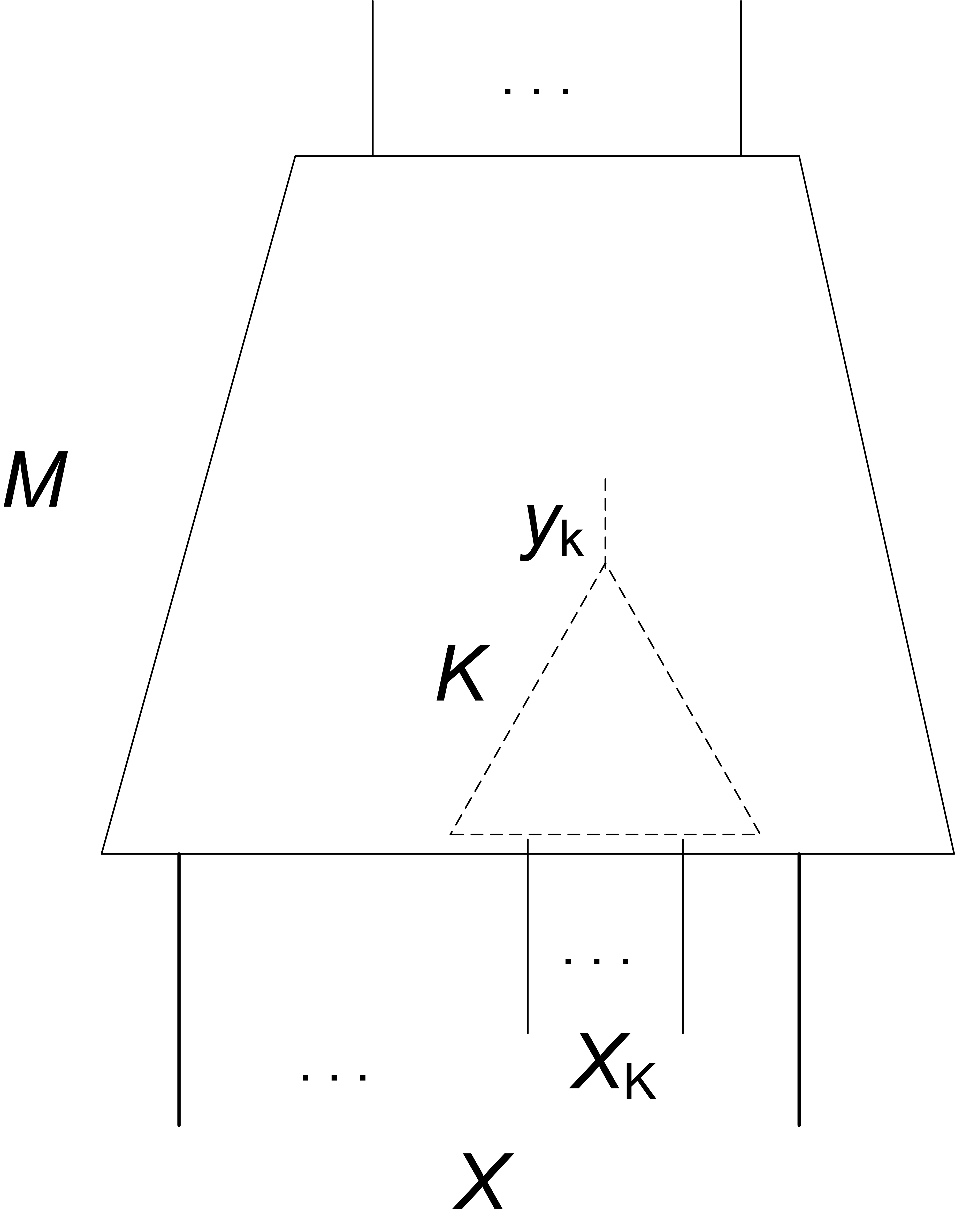
Figure 6: Subcircuit $K$ of circuit $M$

Let $K$ be a single-output subcircuit of circuit $M$ as shown in Figure 6. The input variables of $K$ (set $X_{K}$) is a subset of the input variables of $M$ (set $X$). Suppose that the output of $K$ takes value 0 much more frequently then 1. Then one can view an assignment $\vec{x}$ to $X$ for which $K$ evaluates to 1 as specifying a “corner case” i.e. a rare event. Hitting such a corner case even once by a random test can be very hard. This issue can be addressed by using a coverage metric that requires setting the value of $K$ to both 0 and 1. (The task of finding a test for which $K$ evaluates to 1, can be easily solved, for instance, by using a SAT-solver.) The problem however is that hitting a corner case only once may be insufficient.

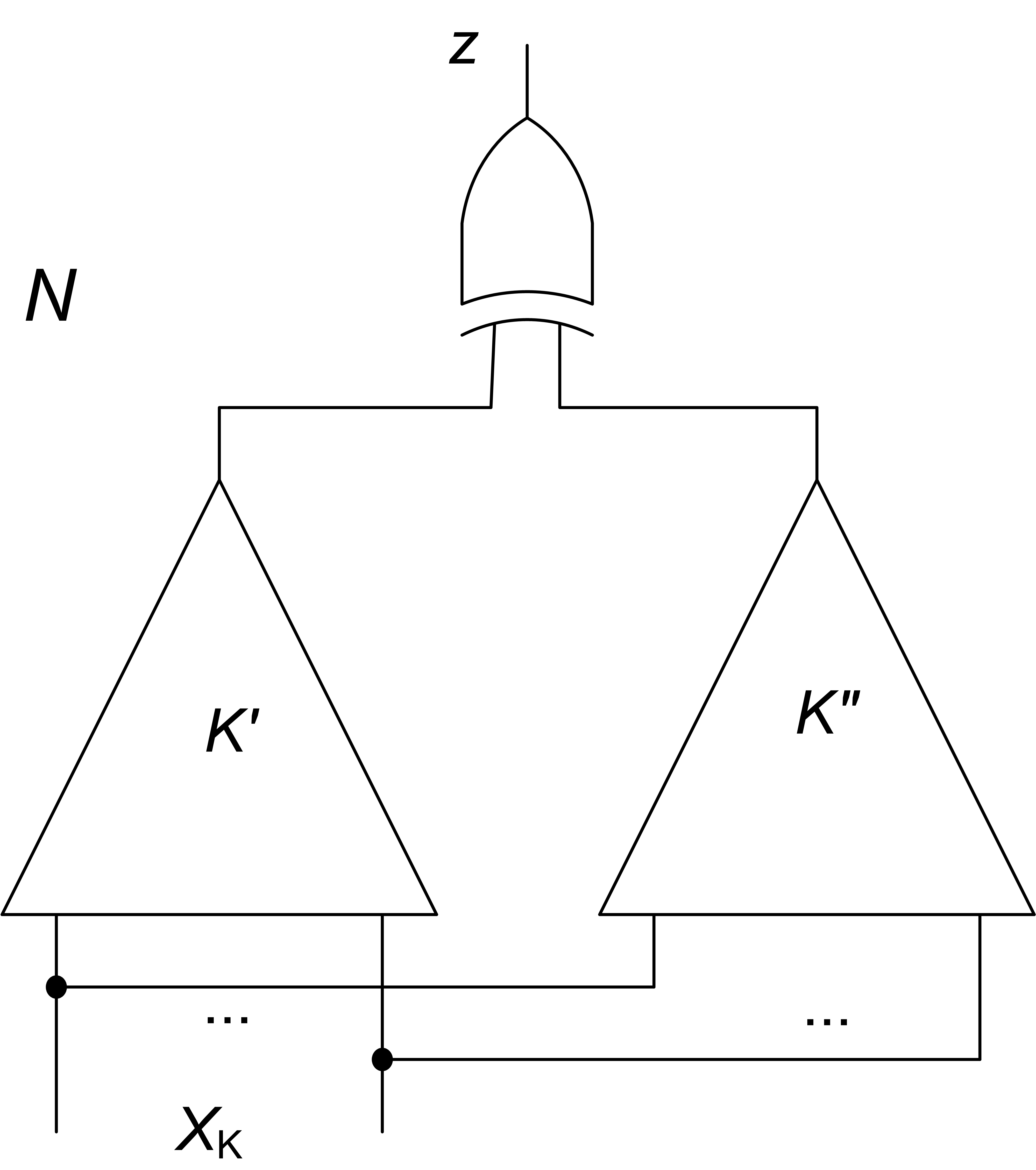
Figure 7: The miter of circuits $K^{\prime}$ and $K^{\prime\prime}$

Ideally, it would be nice to have an option of generating a test set where the ratio of assignments for which $K$ evaluates to 1 is higher than in the truth table of $K$. One can achieve this objective as follows. Let $N$ be a miter of circuits $K^{\prime}$ and $K^{\prime\prime}$ (see Figure 7) i.e. a circuit that evaluates to 1 iff $K^{\prime}$ and $K^{\prime\prime}$ are functionally inequivalent. Let $K^{\prime}$ and $K^{\prime\prime}$ be two copies of circuit $K$. So $N\equiv 0$ holds. Let $T_{K}$ be a CTS for projection of $N$ on $X_{K}$. Set $T_{K}$ can be viewed as a result of “squeezing” the truth table of $K$. Since this truth table is dominated by assignments for which $K$ evaluates to 0, this part of the truth table is reduced the most. So, one can expect that the ratio of tests of $T_{K}$ for which $K$ evaluates to 1 is higher than in the truth table of $K$. In Subsection 8.4, we substantiate this intuition experimentally. Extending an assignment $\vec{x}_{K}$ of $T_{K}$ to an assignment $\vec{x}$ to $X$ is easy e.g. one can randomly assign the variables of $X\setminus X_{K}$.

6.3 Empowering testing by adding CTSs of local properties

Let $\Xi=\mbox{$\{\xi_{1},\dots,\xi_{k}\}$}$ be a set of local properties of $M$ specified by single-output circuits $N_{1},\dots,N_{k}$ respectively. Typically, testing is used to check if circuit $M$ is correct “as a whole”. This notion of correctness is a conjunction of many properties including those of $\Xi$. Let $T$ be a test set generated by a traditional testing procedure (e.g. driven by some coverage metric). An obvious flaw of $T$ is that it does not guarantee that the properties of $\Xi$ hold. This problem can be addressed by using a formal verification procedure, e.g. a SAT-solver, to check if these properties hold. Note, however, that proving the properties of $\Xi$ by a formal verification tool does not add any new tests to $T$ and therefore does not make $T$ more powerful. 1 Now, assume that every property $\xi_{i}$ of $\Xi$ is proved by building a CTS $T_{i}$ for projection of $N_{i}$ on its input variables. Let $T^{*}$ denote $T\cup T_{1}\cup\dots\cup T_{k}$. Set $T^{*}$ is more powerful than $T$ combined with proving the properties of $\Xi$ by a formal verification tool. Indeed, in addition to guaranteeing that the properties of $\Xi$ hold, set $T^{*}$ contains more tests than $T$ and hence can identify new bugs. In Subsection 8.5, we provide some experimental data on using $\mathit{SemStr}$ to verify local properties.

7 Application Of $\mathit{SemStr}$ To Sat-Solving

Conflict Driven Clause Learning (CDCL) [13, 15] has played a major role in boosting the performance of modern SAT-solvers. However, CDCL has the following flaw. Suppose one needs to check satisfiability of formula $G$ equal to $A(X,Y)\wedge B(Y,Z)$ where $|Y|$ is much smaller than $|X|$ and $|Z|$. One can view $G$ as describing interaction of two blocks specified by $A$ and $B$ where $Y$ is the set of variables via which these blocks communicate. Sets $X$ and $Z$ specify the internal variables of these blocks. A CDCL SAT-solver tends to produce clauses that relate variables of $X$ and $Z$ turning $G$ into a “one-block” formula. This can make finding a short proof much harder. (Intuitively, this flaw of CDCL becomes even more detrimental when a formula describes interaction of $n$ small blocks where $n$ is much greater than 2.) A straightforward way to solve this problem is to avoid resolving clauses on variables of $Y$. However, a resolution-based SAT-solver cannot do this. A goal of a resolution proof is to generate an empty clause, which cannot be achieved without resolving clauses on variables of $Y$.

$\mathit{SemStr}$ does not have the problem above since it can just replace resolutions on variables of $Y$ with building an SSA for clauses depending on $Y$. Then, instead of generating an empty clause, $\mathit{SemStr}$ produces an unsatisfiable formula $H(Y)$ implied by $G$. Thus, $\mathit{SemStr}$ can facilitate finding good proofs. However, $\mathit{SemStr}$ has another issue to address. Currently $\mathit{SemStr}$ computes SSAs “explicitly” i.e. in terms of single assignments. The proof system specified by such SSAs is much weaker than resolution. This can negate the positive effect of preserving the structure of $G$. A potential solution of this problem is to compute an SSA in clusters e.g. cubes of assignments where a cube can contain an exponential number of assignments. This makes SSAs a more powerful proof system. (For instance, in [10], the machinery of SSAs is used to efficiently solve pigeon-hole formulas that are hard for resolution.) Computing SSAs in clusters is far from trivial and $\mathit{SemStr}$ can be used as a starting point in this line of research.

8 Experiments

In this section, we describe results of four experiments. In the first experiment (Subsection  8.2), we compute CTSs for circuits and their projections. In Subsection 8.3, we describe the second experiment where $\mathit{SemStr}$ is used for bug detection. In particular, we introduce a method for “piecewise” construction of tests. Importantly, this method has the potential of being as scalable as SAT-solving and so could be used to generate high-quality tests for very large circuits. In the third experiment, (Subsection 8.4) we use CTSs to test corner cases. In the last experiment (Subsection 8.5), we apply $\mathit{SemStr}$ to verification of local properties. In the first three experiments, we used miters i.e. circuits specifying the property of equivalence checking (see Figure 7). In the fourth experiment, we tested circuits specifying the property that an implication between two formulas holds.

8.1 A few remarks about current implementation of $\mathit{SemStr}$

Let $\mathit{SemStr}$ be applied to $G(V,W)$ to produce a formula $H(V)$ and its SSA. As we mentioned in Section 4, when assigning values to variables of $W$, $\mathit{SemStr}$ behaves almost like a regular SAT-solver. So one can use the techniques employed by state-of-the-art SAT-solvers to enhance their performance. However, to make implementation simpler and easier to modify, we have not used those techniques in $\mathit{SemStr}$. For instance, when a variable is assigned a value (implied or decision), a separate node of the search tree is created, no watched literals are used to speed up BCP and so on.

Currently, $\mathit{SemStr}$ does not re-use SSAs obtained in the previous leafs of the search tree. After backtracking, $\mathit{SemStr}$ starts building an SSA from scratch. On the other hand, it is quite possible that, say, an SSA of 100,000 assignments generated in the right branch $w=1$ could have been obtained by making minor changes in the SSA of the left branch $w=0$. Implementation of SSA re-using should boost the performance of $\mathit{SemStr}$ (see Section 0.C of the appendix).

8.2 Computing CTSs for circuits and projections

The objective of the first experiment was to give examples of circuits with non-trivial CTSs and to show that computing a CTS for a projection of $N$ is much more efficient than for $N$. The miter $N$ of circuits $M^{\prime}$ and $M^{\prime\prime}$ (like the one shown in Figure 7 for circuits $K^{\prime}$ and $K^{\prime\prime}$) we used in this experiment was obtained as follows. Circuit $M^{\prime}$ was a subcircuit extracted from the transition relation of an HWMCC-10 benchmark. (The motivation was to use realistic circuits.) For the nine miters we used in this experiment, circuit $M^{\prime}$ was extracted from nine different transition relations. Circuit $M^{\prime\prime}$ was obtained by optimizing $M^{\prime}$ with ABC, a high-quality tool developed at UC Berkeley [18].

The results of the first experiment are shown in Table 1. The first column of Table 1 lists the names of the examples. The second and third columns give the number of input variables and that of gates in $N$. The following group of three columns provide results of computing a CTS for $N$. This CTS was obtained by applying $\mathit{SemStr}$ to formula $F_{N}\wedge z$ with an empty set of variables to exclude. In this case, the resulting formula $H$ is equal to $F_{N}\wedge z$ and $\mathit{SemStr}$ just constructs its SSA. The first column of this group gives the size of the SSA found by $\mathit{SemStr}$. The second column shows the number of different assignments to $X$ in the assignments of this SSA. (Recall that $X$ is the set of input variables of $N$.) The third column of this group gives the run time of $\mathit{SemStr}$. The last two columns of Table 1 describe results of computing CTS for a projection of $N$ on $X$. We will denote this projection by $N^{X}$. This CTS is obtained by applying $\mathit{SemStr}$ to $F_{N}\wedge z$ using $Y\cup z$ as the set of variables to exclude (where $Y$ specifies the set of internal variables of $N$). The first column of the two gives the size of the SSA generated for formula $H(X)$ by $\mathit{SemStr}$. The second column shows the run time of $\mathit{SemStr}$.

Table 1: CTSs for circuits and their projections

name	#inp_	#ga-	CTS for original			CTS for
	vars	tes	circuit			projection
			#SSA	#tests	time	#tests	time
					(s.)		(s.)
ex1	12	54	125,734	500	0.3	28	0.01
ex2	14	59	262,405	3,231	0.6	1,101	0.04
ex3	16	53	438,985	7,211	1.0	867	0.01
ex4	16	63	3,265,861	15,868	9.4	1,452	0.02
ex5	17	66	94,424	952	0.3	137	0.01
ex6	40	117	memout	$*$	$*$	589	0.02
ex7	40	454	memout	$*$	$*$	112,619	5.9
ex8	50	317	memout	$*$	$*$	211,650	4.1
ex9	55	215	memout	$*$	$*$	6,267	0.1

For circuits ex1,..,ex5, $\mathit{SemStr}$ managed to build non-trivial CTSs for the original circuits. Their size is much smaller than $2^{|X|}$. For instance, the trivial CTS for ex5 consists of $2^{17}$=131,072 tests, whereas $\mathit{SemStr}$ found a CTS of 952 tests. (So, to prove $M^{\prime}$ and $M^{\prime\prime}$ equivalent it suffices to run 952 out of 131,072 tests.) For circuits ex6,..,ex9, $\mathit{SemStr}$ failed to build a non-trivial CTS due to memory overflow. On the other hand, $\mathit{SemStr}$ built a CTS for projection $N^{X}$ for all nine examples. Table 1 shows that finding a CTS for $N^{X}$ takes much less time than for $N$. In Subsection 8.3, we demonstrate that although a CTS for $N^{X}$ is only an approximation of a CTS for $N$, it makes a high-quality test set.

8.3 Using CTSs to detect bugs

Table 2: Bug detection

name	#inp_	#ga-	random		test generation
	vars	tes	testing		by $\mathit{SemStr}$
			#tests	time	stra-	#tests	time
			$\times\!10^{6}$	(s.)	tegy		(s.)
ex10	37	73	$>100$	181	1	254	0.02
ex11	39	155	$>100$	466	1	1,742	0.1
ex12	41	591	$>100$	826	1	25,396	2.2
ex13	42	307	$>100$	725	2	4,021	1.1
ex14	50	217	$>100$	489	2	10,147	7.2
ex15	50	249	$>100$	1,290	1	41,048	1.3
ex16	52	1,003	$>100$	707	2	707,589	106
ex17	67	405	$>100$	2,194	2	2,281	1.7
ex18	70	265	$>100$	1,312	2	5,413	0.7

In the second experiment, we used $\mathit{SemStr}$ to generate tests exposing inequivalence of circuits. Let $N^{*}$ denote the miter of circuits $M^{\prime}$ and $M^{\prime\prime}$ where $M^{\prime\prime}$ is obtained from $M^{\prime}$ by introducing a bug. (Similarly to Subsection 8.3, $M^{\prime}$ was extracted from the transition relation of a HWMCC-10 benchmark and for the nine examples of Table 2 below we used nine different transition relations.) Denote by $N$ the miter of circuits $M^{\prime}$ and $M^{\prime\prime}$ where $M^{\prime\prime}$ is just a copy of $M^{\prime}$. In this experiment, we applied the idea of Subsection 6.1: reuse the test set $T$ generated to prove $N\equiv 0$ to test if $N^{*}\equiv 0$ holds. To run a single test $\vec{x}$, we used Minisat 2.0 [7, 19]. Namely, we added unit clauses specifying $\vec{x}$ to formula $F_{N^{*}}\wedge z$ and checked its satisfiability.

To generate $T$ we used two strategies. In strategy 1, $T$ was generated as a CTS for projection $N^{X}$. Strategy 2 was employed when $\mathit{SemStr}$ failed to build a CTS for $N^{X}$ due to memory overflow or exceeding a time limit. In this case, we partitioned $X$ into subsets $X_{1},\dots,X_{k}$ and computed sets $T_{1},\dots,T_{k}$ where $T_{i}$ is a CTS for projection $N^{X_{i}}$. (In the examples where we used strategy 2, the value of $k$ was 2 or 3). The Cartesian product $T_{1}\times\dots\times T_{k}$ forms a test set for $N$. Instead of building the entire set $T$, we randomly generated tests of $T$ one by one as follows. The next test $\vec{x}$ of $T$ to try was formed by taking the union of ${\mbox{$\vec{x}$}}_{i}$,$i=1,\dots,k$ randomly picked from corresponding $T_{i}$,$i=1,\dots,k$. Note that in the extreme case where every $X_{i}$ consists of one variable, strategy 2 reduces to generation of random tests. Indeed, let $X_{i}=\mbox{$\{x_{i}\}$}$,$i=1,\dots,k$ where $k=|X|$. Then formula $H(X_{i})$ for projection $N^{X_{i}}$ is equal to $x_{i}\wedge\overline{x}_{i}$. The only SSA for $H(X_{i})$ is trivial and consists of assignments $x_{i}=0$ and $x_{i}=1$ (and so does $T_{i}$). By randomly choosing a test of $T_{i}$ one simply randomly assigns 0 or 1 to $x_{i}$.

Figure 8: Circuit $K$ whose output value is biased to 0

We compared our approach with random testing on small circuits. Our objective was to show that although random testing is much more efficient (test generation is very cheap), testing based on CTSs is much more effective. The majority of faults we tried was easy for both approaches. In Table 2, we list some examples that turned out to be hard for random testing. The first three columns are the same as in Table 1. The next two columns describe the performance of random testing: the number of tests we tried (in millions) and the time taken by Minisat to run all tests. The last three columns describe the performance of our approach. The first column of these three shows whether strategy 1 or 2 was used. The second column gives the number of tests from $T$ one needed to run before finding a bug. (Thus, this number is smaller than $|T|$.) The last column of these three shows the total run-time that consists of the time taken by $\mathit{SemStr}$ to generate $T$ and the time taken by Minisat to run tests.

Table 2 shows that tests extracted from CTSs for projections of $N$ are very effective. The fact that these tests are effective even for strategy 2 is very encouraging for the following reason. Computing a CTS for a projection $N^{V}$ where $V$ is small is close to regular SAT-solving. (They become identical if $V=\emptyset$.) Implementation of improvements mentioned in Subsection 8.1 should make computing a CTS for $N^{V}$ almost as scalable as SAT-solving. Thus, by breaking $X$ into relatively small subsets $X_{1},\dots,X_{k}$ and using piecewise construction of tests as described above, one will get an effective test set that can be efficiently computed even for very large circuits.

8.4 Using CTSs to check corner cases

Table 3: Using CTSs for checking corner cases

name	#inp_	and	#ga-	random testing			test generation
	vars	inps	tes				by $\mathit{SemStr}$
				#te-	#hi-	time	#te-	#hits	time
				sts	ts	(s.)	sts		(s.)
ex19	50	10	72	$10^{5}$	54	0.6	832	51	0.03
ex19*	60	20	72	$10^{7}$	0	65	1,803	207	0.1
ex20	50	10	160	$10^{5}$	5	1.3	21,496	1,303	0.4
ex20*	60	20	160	$10^{7}$	0	129	161,195	10,036	3.1
ex21	65	10	108	$10^{5}$	68	0.8	49,947	4,168	1.2
ex21*	75	20	108	$10^{7}$	0	81	44,432	3,528	1.2
ex22	51	10	296	$10^{5}$	81	1.8	50,388	4,560	4.9
ex22*	61	20	296	$10^{7}$	0	184	235,452	22,326	26
ex23	60	10	125	$10^{5}$	43	1.2	6,834	259	0.2
ex23*	70	20	125	$10^{7}$	0	122	21,083	1,807	0.4

In the third experiment, we used CTSs to test corner cases (see Subsection 6.2). First we formed a circuit $K$ that evaluates to 0 for almost all input assignments. So the input assignments for which $K$ evaluates to 1 specify “corner cases”. Then we compared the frequency of hitting the corner cases of $K$ by random testing and by tests of a set $T$ built by $\mathit{SemStr}$. The test set $T$ was obtained as follows. Let $N$ be the miter of copies $K^{\prime}$ and $K^{\prime\prime}$ (see Figure 7). Set $T$ was generated as a CTS for the projection of $N$ on its input variables.

Circuit $K$ was formed as follows. First, we extracted a circuit $R$ as a subcircuit of a transition relation (as described in the previous subsections). Then we formed circuit $K$ by composing an n-input AND gate and circuit $R$ as shown in Figure 8. Circuit $K$ outputs 1 only if $R$ evaluates to 1 and the first $n-1$ inputs variables the AND gate are set to 1 too. So the input assignments for which $K$ evaluates to 1 are “corner cases”.

The results of our experiment are given in Table 3. The first column specifies the name of an example. The next two columns give the total number of input variables of $K$ and the number of input variables in the multi-input AND gate (see Figure 8). The next three columns describe the performance of random testing. The first column of the three gives the total number of tests. The next column shows the number of times circuit $K$ evaluated to 1 (i.e. a corner case was hit). The last column of the three gives the total run time. The last three columns of Table 3 describe the results of $\mathit{SemStr}$. The first column of the three shows the size of a CTS generated as described above. The next column gives the number of times a corner case was hit. The last column shows the total run time (that also includes the time used to generate the CTS).

The examples of Table 3 were generated in pairs that shared the same circuit $R$ and were different only the size of the AND gate (see Figure 8). For instance, in ex19 and ex19* we used 10-input and 20-input AND gates respectively. Table 3 shows that for circuits with 10-input AND gates, random testing was able to hit corner cases but the percentage of those events was very low. For instance, for ex19, only for 0.05% of tests the output value of $K$ was 1 (54 out of $10^{5}$ tests). The same ratio for tests generated by $\mathit{SemStr}$ was 6.12% (51 out of 832 tests). A significant percentage of tests generated by $\mathit{SemStr}$ hit corner cases even in examples with 20-input AND gates in sharp contrast to random testing that failed to hit a single corner case.

8.5 Using CTSs to verify local properties

In the last experiment, we used $\mathit{SemStr}$ to build CTSs for local properties (see Subsection 6.3). Our objective here was just to show that even the current implementation of $\mathit{SemStr}$ was powerful enough to generate CTSs for local properties of non-trivial circuits.

Table 4: Tests for local properties

HWMCC-10	#inp_	#lat-	#gates	$|C|$	#tests	time
benchmark	vars	ches				s.
nusmvbrp	11	52	518	3	8,690	0.7
cmugigamax	34	29	646	4	1,158	0.2
kenoopp1	49	51	619	2	84	0.5
kenflashp01	61	57	1,292	7	46	0.9
nusmvguidancep1	84	86	1,823	3	767	1.2
visprodcellp01	30	78	2,807	2	534	1.4
pdtswvroz10x6p1	7	81	3,088	4	76	0.1
pdtvissoap2	21	205	4,333	2	6,408	1.6
pdtvissfeistel	68	361	9,976	2	5,078	0.1

In the experiment, we tested local properties defined as follows. Let $M_{T}$ be a combinational circuit specifying a transition relation $T(X,S,Y,S^{\prime})$. Here $S$ and $S^{\prime}$ are sets of the present and next state variables, and $X$ and $Y$ are sets of the combinational input and internal variables respectively. So $X\cup S$ and $S^{\prime}$ specify the input and output variables of $M_{T}$ respectively. Let $P$ be a set of clauses specifying an inductive invariant for $T$. That is $P(S)\wedge T\rightarrow P(S^{\prime})$. Let $C$ be a clause of $P$. Then $P(S)\wedge T\rightarrow C(S^{\prime})$. This implication can be viewed as a property of circuit $M_{T}$. We will refer to it as a property specified by clause $C$ (and predicate $P$). It states that for every input assignment satisfying $P$, the output assignment of $M_{T}$ satisfies $C$. Typically, $C$ is a short clause i.e. the number of literals of $C$ is much smaller than $|S^{\prime}|$. If only a small part of $M_{T}$ feeds the output variables present in $C$, then the property specified by $C$ is local.

Table 4 shows the results of our experiment. The first column gives the name of an HWMCC-10 benchmark specified by $M_{T}$. The next three columns show the number of input combinational variables, state variables and gates in $M_{T}$. The next column gives the number of literals of clause $C$ randomly picked from an inductive invariant (generated by IC3 [2]). The last two columns describe the results of $\mathit{SemStr}$ in building a CTS for a projection of circuit $N$ defined in Footnote 10 on the set of input variables (i.e. on $X\cup S$). These columns describe the size of the CTS and the run time taken by $\mathit{SemStr}$ to build it. Table 4 shows that $\mathit{SemStr}$ managed to build CTSs for local properties of non-trivial circuits (e.g. for circuit pdtvissfeistel that has 9,976 gates and 361 latches).

9 Background

As we mentioned earlier, the objective of applying a test to a circuit is typically to check if the output assignment produced for this test is correct. This notion of correctness usually means satisfying the conjunction of many properties of this circuit. For that reason, one tries to spray tests uniformly in the space of all input assignments. To avoid generation of tests that for some reason should be or can be excluded, a set of constraints can be used [12]. Another way to improve the effectiveness of testing is to run many tests at once as it is done in symbolic simulation [3]. Our approach is different from those above in that it is “property-directed” and hence can be used to generate property-specific tests.

The method of testing introduced in [11] is based on the idea that tests should be treated as a “proof encoding” rather than a sample of the search space. (The relation between tests and proofs have been also studied in software verification, e.g. in [8, 9, 1]). A flaw of this approach is that testing is treated as a second-class citizen whose quality can be measured only by a formal proof it encodes. In this paper, we take a different point of view where testing becomes the part of a formal proof that performs structural derivations.

In [14], it was shown that Craig’s interpolation [4] can be used in model checking. An efficient procedure for extraction of an interpolant from a resolution proof was given in [17, 14]. A flaw of this procedure is that the size of this interpolant strongly depends on the quality of the proof. As we mentioned in Section 7, $\mathit{SemStr}$ offers a new way to solve formulas with structure. In particular, $\mathit{SemStr}$ can be used to compute interpolants. Let formula $G(X,Y,Z)$ be equal to $A(X,Y)\wedge B(Y,Z)$ and one applies $\mathit{SemStr}$ to solve formula $G$ by excluding the variables of $X\cup Z$. Then formula $H(Y)$ produced from $G$ by $\mathit{SemStr}$ can be represented as $H_{1}\wedge H_{2}$ where $H_{1}$ and $H_{2}$ are interpolants for $A$ and $B$ respectively. That is $A\rightarrow H_{1}\rightarrow\overline{B}$ and $B\rightarrow H_{2}\rightarrow\overline{A}$. (This is due to the fact that $\mathit{SemStr}$ forbids resolutions on variables of $Y$.) An advantage of $\mathit{SemStr}$ is that it takes into account formula structure and hence can potentially produce high-quality interpolants. However, currently, using $\mathit{SemStr}$ for interpolant generation does not scale as well as extraction of an interpolant from a proof.

Reasoning about SAT in terms of random walks was pioneered in [16]. The centered SSAs we introduce in this paper bear some similarity to sets of assignments generated in de-randomization of Schöning’s algorithm [5]. Typically, centered SSAs are much smaller than uncentered SSAs introduced in [10]. A big advantage of the uncentered SSA though is that its definition facilitates computing an SSA in clusters of assignments (rather than single assignments).

10 Conclusion

We consider the problem of finding a Complete Test Set (CTS) for a combinational circuit $N$ that is a test set proving that $N\equiv 0$. We use the machinery of stable sets of assignments to derive non-trivial CTSs i.e. ones that do not include all possible input assignments. The existence of non-trivial CTSs implies that it is more natural to consider testing as structural rather than semantic derivation (the former being derivation of a property that cannot be expressed in terms of the truth table). Since computing a CTS for the entire circuit $N$ is impractical, we present a procedure called $\mathit{SemStr}$ that computes a CTS for a projection of $N$ on a subset of its variables. The importance of $\mathit{SemStr}$ is twofold. First, it can be used for generation of effective test sets. In particular, we describe a procedure for “piecewise” construction of tests that can be potentially applied to very large circuits. Second, $\mathit{SemStr}$ can be used as a starting point in designing verification tools that efficiently combine structural and semantic derivations.

Appendix

Appendix 0.A Proofs

Proposition 1

Formula $H$ is unsatisfiable iff it has an SSA.

Proof

If part. Assume the contrary. Let $P$ be an SSA of $H$ with center $\vec{p}_{\mathit{init}}$ and $H$ is satisfiable. Let $\vec{s}$ be an assignment satisfying $H$. Let $\vec{p}$ be an assignment of $P$ that is the closest to $\vec{s}$  in terms of the Hamming distance. Let $C=\mbox{$\Phi$}({\mbox{$\vec{p}$}})$. Since $\vec{s}$ satisfies clause $C$, there is a variable $v\in\mbox{$\mathit{Vars}(C)$}$ that is assigned differently in $\vec{p}$ and $\vec{s}$. Let $\vec{p^{*}}$ be the assignment obtained from $\vec{p}$ by flipping the value of $v$. Note that ${\mbox{$\vec{p^{*}}$}}\in\mathit{Nbhd}(\mbox{$\vec{p}_{\mathit{init}}$},{\mbox{$\vec{p}$}},C)$.

Assume that ${\mbox{$\vec{p^{*}}$}}\in P$. In this case, $\vec{p^{*}}$ is closer to $\vec{s}$ than $\vec{p}$ and we have a contradiction. Now, assume that ${\mbox{$\vec{p^{*}}$}}\not\in P$. In this case, $\mathit{Nbhd}(\mbox{$\vec{p}_{\mathit{init}}$},{\mbox{$\vec{p}$}},C)\not\subseteq P$ and so set $P$ is not an SSA. We again have a contradiction.

Only if part. Assume that formula $H$ is unsatisfiable. By applying BuildSSA shown in Figure 2 to $H$, one generates a set $P$ that is an SSA of $H$ with respect to some center $\vec{p}_{\mathit{init}}$ and AC-mapping $\Phi$.

Appendix 0.B CTSs And Circuit Redundancy

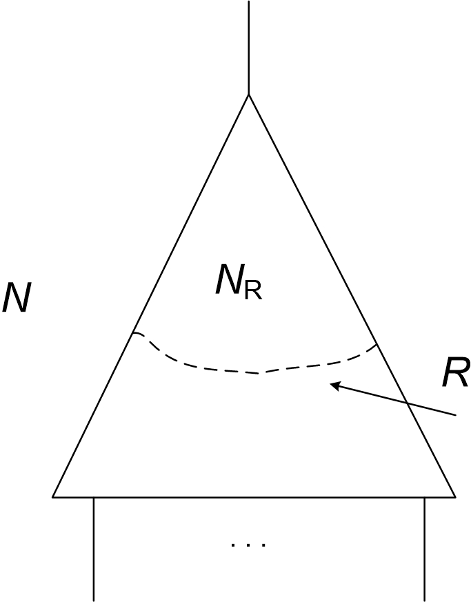
Figure 9: A cut $R$ in circuit $N$

Let $N\equiv 0$ hold. Let $R$ be a cut of circuit $N$. We will denote the circuit between the cut and the output of $N$ as $N_{R}$ (see Figure 9). We will say that $N$ is non-redundant if $N_{R}\not\equiv 0$ for any cut $R$ other than the cut specified by primary inputs of $N$.

Definition 3 of a CTS may not work well if $N$ is highly redundant. Assume, for instance, that $N_{R}\equiv 0$ holds for cut $R$. This means that the clauses specifying gates of $N$ below cut $R$ (i.e. ones that are not in $N_{R}$) are redundant in $F_{N}\wedge z$. Then one can build an SSA $P$ for $F_{N}\wedge z$ as follows. Let $P_{R}$ be an SSA for $F_{N_{R}}\wedge z$. Let $\vec{v}$ be an arbitrary assignment to the variables of $\mbox{$\mathit{Vars}(N)$}\setminus\mbox{$\mathit{Vars}(N_{R})$}$. Then by adding $\vec{v}$ to every assignment of $P_{R}$ one obtains an SSA for $F_{N}\wedge z$. This means that for any test $\vec{x}$, $\mathit{Cube}({\mbox{$\vec{x}$}})$ contains an SSA of $F_{N}\wedge z$. Therefore, according to Definition 3, circuit $N$ has a CTS consisting of just one test.

The problem above can be solved using the following observation. Let $T$ be a set of tests $\{{\mbox{$\vec{x}_{1}$}},\dots,{\mbox{$\vec{x}_{k}$}}\}$ for $N$ where $k\leq 2^{|X|}$. Denote by $\vec{r}_{i}$ the assignment to the variables of cut $R$ produced by $N$ under input $\vec{x}_{i}$. Let $T_{R}$ denote $\{{\mbox{$\vec{r}_{1}$}},\dots,{\mbox{$\vec{r}_{k}$}}\}$. Denote by $T^{*}_{R}$ the set of assignments to variables of $R$ that cannot be produced in $N$ by any input assignment. Now assume that $T$ is constructed so that $T_{R}\cup T^{*}_{R}$ is a CTS for circuit $N_{R}$. This does not change anything if $N_{R}$ is itself redundant (i.e. if $N_{R^{\prime}}\equiv 0$ for some cut $R^{\prime}$ that is closer to the output of $N$ than $R$). In this case, it is still sufficient to use $T$ of one test because $N_{R}$ has a CTS of one assignment (in terms of cut $R$). Assume however, that $N_{R}$ is non-redundant. In this case, there is no “degenerate” CTS for $N_{R}$ and $T$ has to contain at least $|T_{R}|$ tests. Assuming that $T^{*}_{R}$ alone is far from being a CTS for $N_{R}$, a CTS $T$ for $N$ will consist of many tests.

So a solution to the problem caused by redundancy of $N$ is as follows. One should require that for every cut $R$ where $N_{R}\equiv 0$ holds, set $T_{R}\cup T^{*}_{R}$ should be a CTS for $N_{R}$. The fact that there always exists at least one cut $R$ where $N_{R}$ is non-redundant eliminates degenerate single-test CTSs for $N$.

Appendix 0.C Reusing SSAs

Let $\mathit{SemStr}$ be applied to formula $G(V,W)$ to produce formula $H(V)$ and its SSA. Let us explain the idea of SSA reusing by the following example. Let $P_{0}$ be the SSA generated by $\mathit{SemStr}$ in branch $w=0$ where $w\in W$. Let us show how SSA $P_{1}$ for branch $w=1$ can be derived from $P_{0}$. Let $\mbox{$\Phi$}_{0}$ be the AC-mapping for $P_{0}$. Assume for the sake of simplicity that

• only one clause $B$ of $\mbox{$\Phi$}_{0}(P_{0})$ contains literal $w$

• only assignment ${\mbox{$\vec{q}$}}\in P_{0}$ is mapped by $\mbox{$\Phi$}_{0}$ to clause $B$.

Thus, the only reason why $P_{0}$ is not an SSA in branch $w=1$ is that $\vec{q}$ is not mapped to any clause. (Recall that SSAs built by $\mathit{SemStr}$ consist of assignments to $V$. So the construction of an SSA in branch $w=1$ is different from $w=0$ only because some $V$-clauses of branch $w=0$ are satisfied in branch $w=1$ and vice versa.) Let BuildSSA* denote the modification of procedure BuildSSA (see Figure 2) aimed at re-using $P_{0}$ when building SSA $P_{1}$.

Recall that BuildSSA maintains sets $E$ and $Q$. The former consists of the assignments whose neighborhood has been already explored and the latter stores the assignments whose neighborhood is yet to be explored. BuildSSA* splits $Q$ into two sets: $Q^{\prime}$ and $Q^{\prime\prime}$. An assignment $\vec{p}$ is put in $Q^{\prime}$ if

• $\vec{p}$ is in $P_{0}$ and

• clause $\mbox{$\Phi$}_{0}({\mbox{$\vec{p}$}})$ is not satisfied by $w=1$

(In our case, every assignment of $P_{0}$ but the assignment $\vec{q}$ above is put in set $Q^{\prime}$.) On the other hand, every assignment whose neighborhood is yet to be considered and that does not satisfy the two conditions above is put in set $Q^{\prime\prime}$. The reason for this split is that the assignments from $Q^{\prime}$ are cheaper to process. Namely, if ${\mbox{$\vec{p}$}}\in Q^{\prime}$, then instead of looking for a clause falsified by $\vec{p}$, BuildSSA* uses clause $\mbox{$\Phi$}_{0}({\mbox{$\vec{p}$}})$. For that reason, assignments of $Q^{\prime}$ are the first to be considered by BuildSSA*. An assignment of $Q^{\prime\prime}$ is processed only if $Q^{\prime}$ is currently empty.

BuildSSA* starts with the same center $\vec{p}_{\mathit{init}}$ that was used when building $P_{0}$. If $\vec{p}_{\mathit{init}}$ is different from $\vec{q}$, it is put in $Q^{\prime}$. Otherwise, it is put in $Q^{\prime\prime}$. Let $\vec{p}$ be the assignment picked by BuildSSA* from $Q^{\prime}$ or $Q^{\prime\prime}$. Let $C$ be the clause to which $\vec{p}$ is mapped by $\mbox{$\Phi$}_{1}$. Let $\vec{p^{*}}$ be an assignment of $\mathit{Nbhd}(\mbox{$\vec{p}_{\mathit{init}}$},{\mbox{$\vec{p}$}},C)$. If $\vec{p^{*}}$ satisfies the two conditions above, BuildSSA* puts it in $Q^{\prime}$. Otherwise, $\vec{p^{*}}$ is added to $Q^{\prime\prime}$.

References

- [1] N. Beckman, A. Nori, S. Rajamani, R. Simmons, S. Tetali, and A. Thakur. Proofs from tests. IEEE Transactions on Software Engineering, 36(4):495–508, July 2010.
- [2] A. R. Bradley. Sat-based model checking without unrolling. In VMCAI, pages 70–87, 2011.
- [3] R. Bryant. Symbolic simulation—techniques and applications. In DAC-90, pages 517–521, 1990.
- [4] W. Craig. Three uses of the herbrand-gentzen theorem in relating model theory and proof theory. The Journal of Symbolic Logic, 22(3):269–285, 1957.
- [5] E. Dantsin, A. Goerdt, E. Hirsch, R. Kannan, J. Kleinberg, C. Papadimitriou, P. Raghavan, and U. Schöning. A deterministic (2−2/(k+1))n algorithm for k-sat based on local search. Theoretical Computer Science, 289(1):69 – 83, 2002.
- [6] M. Davis, G. Logemann, and D. Loveland. A machine program for theorem proving. Communications of the ACM, 5(7):394–397, July 1962.
- [7] N. Eén and N. Sörensson. An extensible sat-solver. In SAT, pages 502–518, Santa Margherita Ligure, Italy, 2003.
- [8] C. Engel and R. Hähnle. Generating unit tests from formal proofs. In TAP, pages 169–188, 2007.
- [9] P. Godefroid and N. Klarlund. Software model checking: Searching for computations in the abstract or the concrete. In Integrated Formal Methods, pages 20–32, 2005.
- [10] E. Goldberg. Testing satisfiability of cnf formulas by computing a stable set of points. In Proc. of CADE-02, pages 161–180, 2002.
- [11] E. Goldberg. On bridging simulation and formal verification. In VMCAI-08, pages 127–141, 2008.
- [12] N. Kitchen and A.Kuehlmann. Stimulus generation for constrained random simulation. In ICCAD-07, pages 258–265, 2007.
- [13] J. Marques-Silva and K. Sakallah. Grasp – a new search algorithm for satisfiability. In ICCAD-96, pages 220–227, 1996.
- [14] K. L. Mcmillan. Interpolation and sat-based model checking. In CAV-03, pages 1–13. Springer, 2003.
- [15] M. Moskewicz, C. Madigan, Y. Zhao, L. Zhang, and S. Malik. Chaff: engineering an efficient sat solver. In DAC-01, pages 530–535, New York, NY, USA, 2001.
- [16] C. H. Papadimitriou. On selecting a satisfying truth assignment. In 32nd Annual Symposium of Foundations of Computer Science, pages 163–169, Oct 1991.
- [17] P. Pudlak. Lower bounds for resolution and cutting plane proofs and monotone computations. Journal of Symbolic Logic, 62(3):981–998, 1997.
- [18] Berkeley Logic Synthesis and Verification Group. ABC: A system for sequential synthesis and verification, 2017. http://www.eecs.berkeley.edu/alanmi/abc.
- [19] Minisat2.0. http://minisat.se/MiniSat.html.