mQAPViz: A divide-and-conquer multi-objective optimization algorithm to compute large data visualizations

Abstract.

Algorithms for data visualizations are essential tools for transforming data into useful narratives. Unfortunately, very few visualization algorithms can handle the large datasets of many real-world scenarios. In this study, we address the visualization of these datasets as a Multi-Objective Optimization Problem. We propose mQAPViz, a divide-and-conquer multi-objective optimization algorithm to compute large-scale data visualizations. Our method employs the Multi-Objective Quadratic Assignment Problem (mQAP)as the mathematical foundation to solve the visualization task at hand. The algorithm applies advanced sampling techniques originating from the field of machine learning and efficient data structures to scale to millions of data objects. The algorithm allocates objects onto a 2D grid layout. Experimental results on real-world and large datasets demonstrate that mQAPViz is a competitive alternative to existing techniques.

1. Introduction

While we read this sentence, terabytes of data have been collectively generated across the globe through many devices we use daily. Exploratory Data Analysis (EDA)is a critical first stage to investigate datasets. The techniques that enable EDA provide a summarized view of a whole dataset. In particular, visualization algorithms play a relevant role in these tasks. They may capture some of the inherent hidden characteristics and structures, presenting them in such a way that allow transforming raw data into actionable insights.

Displaying data is a non-trivial task considering that we aim to summarize complex relationships between objects in a human-readable layout (i.e., 2D or 3D). Visualization techniques are well suited for small (hundreds) and medium (thousands) size datasets. However, the task is even more challenging today considering the scale of the datasets in need of these algorithms. Data products have been an instrumental part of big technological companies. Large institutions have the human capital and the computational infrastructures to conduct big analyses on massively distributed systems. However, there are many researchers and practitioners who do not have access to these platforms. They would benefit from a new generation of more efficient algorithms that can compute visualizations of large datasets on modern multi-core workstation computers.

Typically, EDA is used to collect new insights from independent views obtained from the data. We argue however that algorithms devoted to data analysis should take into account several viewpoints to evaluate relations. Multi-objective optimization algorithms have been widely proposed and used to address real-world Multi-Objective Optimization Problems (MOPs)(Deb, 2001). In MOPs, the challenge is to simultaneously satisfy multiple and possibly conflicting objectives.

In multi-objective optimization problems, there is not a unique solution, but a set of non-dominated solutions (i.e., a trade-off in the objective space) which is called the Pareto optimal set. Multi-Objective Evolutionary Algorithms (MOEAs)are well-suited to approximate the Pareto optimal set in a broad variety of MOPs (Zitzler and Thiele, 1999). MOEAs evolve individuals (solutions) typically organized in populations, exploring the solution space using operators such as recombination, mutation, and selection to improve the population.

In this study, we propose mQAPViz (pronounced mapviz), a novel multi-objective optimization algorithm to compute visualizations of large-scale datasets. Our algorithm employs the Multi-Objective Quadratic Assignment Problem, which is presented in the following sections, as the mathematical model to position objects in a grid layout. To the best of our knowledge, this study is the first one that addresses the visualization of large datasets as a Multi-Objective Optimization Problem. In particular, we present the following contributions:

• We propose mQAPViz, a new multi-objective optimization algorithm which can compute large-scale data visualizations.

• We propose a divide-and-conquer approach to solve sub-problems of the Multi-Objective Quadratic Assignment Problem to tackle the visualization task at hand.

• We evaluate our approach on a set of large and real datasets that belong to different domains against the state-of-the-art visualization algorithm t-SNE.

We organize the remainder of the paper as follows. In Section 2, we discuss the related work. We present the details of mQAPViz in Section 3. We discuss our experimental methodology and the results in Section 4. We finish with the conclusions and future work in Section 5.

2. Related Work

Data visualizations assist the process of representing data for supporting the tasks of exploration, confirmation, presentation, and understanding to deliver knowledge (Few, 2009). Several tools and algorithms have been developed over the years. For example, force-directed layout algorithms use a graph data structure to model datasets as a dynamical system. Nodes represent mutually repelling particles, and edges correspond to the existence of an attractive force between them. The layout is determined once the forces drive the system to equilibrium (Fruchterman and Reingold, 1991).

Other approaches organize objects in a grid layout. These methods produce a visualization using a finite number of positions defined by a grid. For example, the grid layout has been used to visualize biochemical networks (Li and Kurata, 2005). Another general method for data visualization using a grid layout is presented in (Abbiw-Jackson et al., 2006) in which the authors proposed a divide-and-conquer method that recursively distributes the data in grids. Later, QAPgrid was proposed in (Inostroza-Ponta et al., 2011) which using the Quadratic Assignment Problem (QAP)as the mathematical model, a proximity graph, and a single-objective optimization guides the generation of a grid layout of objects. The method has been used in several applications (Clark et al., 2012; Warren et al., 2017), but its current version cannot compute large datasets (i.e., millions of objects) in a reasonable time.

Data visualization can also be seen as the task of mapping data from a high-dimensional to a low-dimensional space using some distance-preserving dimensionality reduction in the final representation. Traditional methods in the literature include Principal Component Analysis (PCA)or Linear Discriminant Analysis (LDA). Other well-known algorithms use the hypothesis that the data can be approximated by a low-dimensional manifold, such as Laplacian Eigenmaps (Belkin and Niyogi, 2003), Isomap (Tenenbaum et al., 2000) or Local Linear Embedding (LLE) (Roweis and Saul, 2000). We refer to Ref. (Van Der Maaten et al., 2009) in which the authors presented a comparative study of dimensionality reduction techniques.

A handful of visualization algorithms can efficiently address the challenges of large-scale datasets. In particular, two successful algorithms (Van Der Maaten, 2014; Tang et al., 2016) that aim at closing this gap share two characteristics: efficient data structures and ad-hoc probabilistic models. The popular t-SNE method minimizes the divergence between a distribution that measures pairwise similarities of the input objects and a distribution that measures pairwise similarities of the corresponding low-dimensional representation. LargeVis implements an approximate $k$-nearest neighbor graph and graph sampling techniques, improving the original complexity from $\mathcal{O}(n~{}log~{}n)$ to $\mathcal{O}(n)$ (in which $n$ is the number of samples in the dataset). In the following sections, we present mQAPViz which integrates ideas taken from the multi-objective optimization domain to compute large data visualizations.

3. A multi-objective optimization algorithm to compute large data visualizations

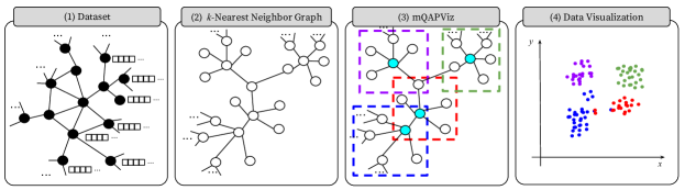
Figure 1. An illustration of the workflow involved in mQAPViz.

In this section we present mQAPViz, a new multi-objective algorithm to generate visualizations of large-scale datasets.

3.1. The Multi-Objective Quadratic Assignment Problem approach data visualization

Formally, the special case of the Multi-Objective Quadratic Assignment Problem (mQAP)in which the number of objects is the same to the number of positions ($n$) is defined as follows:

(1) $$\underset{\pi\in P_{n}}{\text{minimize}}\;\;C(\pi) =\{C_{1}(\pi),C_{2}(\pi),...,C_{k}(\pi)\}$$

$$C_{r}(\pi) =\sum_{i=1}^{n}\sum_{j=1}^{n}d_{ij}f^{r}_{\pi(i)\pi(j)},\>r=1,\dots,k~{},$$

where $f^{r}_{\pi(i)\pi(j)}$ represents the flow between the object $\pi(i)=p$ and $\pi(j)=q$ of the $r$-th flow and $d_{ij}$ is the distance between the position $i$ and $j$. $P_{n}$ represents the set of all permutations $\pi:N\rightarrow N$. The product $d_{ij}\,f^{r}_{\pi(i)\pi(j)}$ corresponds to the $r$-th cost of allocating object $\pi(i)=p$ to the position $i$ and object $\pi(j)=q$ to the position $j$. The difference between mQAP and the single-objective Quadratic Assignment Problem (QAP)is that we consider more than one flow (i.e., $k$ flows in Equation 1), and we minimize them simultaneously.

Using the QAP as a proxy for data visualization is a simple and intuitive idea. First, we create a layout with available positions to allocate the objects. We can create a human-readable layout to visualize a dataset with $n$ objects using a low-dimensional grid with $m$ possible positions ($n<<m$). Second, we allocate the objects into the layout with the aim of minimizing the cost which is a function of the distances and the flows. Intuitively, similar objects should be positioned closer to each other and dissimilar objects should be pushed away. We may define a (dis)similarity measure depending on the particular domain of study. Although this approach has shown relatively good results in datasets with thousands of objects (Inostroza-Ponta et al., 2011), it is impractical for large-scale datasets, and our contribution is addressing this need.

3.2. mQAPViz

To compute visualizations of large datasets, we use a divide-and-conquer strategy which creates and solves several mQAP instances. These sub-instances represent a sampled portion of the whole dataset. Our method is based on two main components. An initial layout is created, and later it is optimized thanks to a mQAP-based approach. For this second part, we compute a k-Nearest Neighbors Graph (k-NNG)which is used to obtain information about the most similar sets of the data objects. Then, a sampling strategy is used to select a set of nodes that will be used to create mQAP sub-instances to be optimized. Each sub-instance is optimized thanks to our method called PasMoQAP (Sanhueza et al., 2017), a parallel asynchronous memetic algorithm. Finally, we merge the individual solutions to create several visualizations in a low-dimensional space.

The Figure 1 illustrates the workflow involved in mQAPViz (Algorithm 1). In the next sections, we discuss the details of the main components implemented in mQAPViz.

Algorithm 1 Pseudo-code of mQAPViz

1:dataset $D$, number of trees $n_{t}$, number of neighbors $k$, number of iterations $it$, portion of sampled nodes $p_{s}$

2:Final set of visualizations $L_{f}$

3:$\mathcal{P}^{*}\leftarrow\emptyset$ $\triangleright$ Set of individual solutions

4:$G_{k-nn}\leftarrow\textsc{BuildKNNG}(D,n_{t},k,it)$ $\triangleright$ See Algorithm 2

5:$L_{0}\leftarrow\textsc{LargeVis}(D,G_{k-nn})$

6:$V_{s}\leftarrow\textsc{NegativeSampling}(G_{k-nn},p_{s})$

7:for each vertex $v_{i}\in V_{s}$ in parallel do $\triangleright$ Solving mQAP instances

8:    $I_{v_{i}}\leftarrow\textsc{CreateMQAPVisInstance}(G_{k-nn},v_{i})$

9:    $\mathcal{P}^{*}_{v_{i}}\leftarrow\textsc{PasMoQAP}(I_{v_{i}})$

10:    $\mathcal{P}^{*}\leftarrow\mathcal{P}^{*}\cup\mathcal{P}^{*}_{v_{i}}$

11:end for

12:$V_{s}\leftarrow\emptyset$

13:$V_{s}\leftarrow\textsc{GetMissingVertices}(\mathcal{P}^{*})$ $\triangleright$ Getting vertices without an assigned position

14:for each vertex $v_{i}\in V_{s}$ in parallel do

15:    $I_{v_{i}}\leftarrow\textsc{CreateMQAPInstance}(G_{k-nn},v_{i})$

16:    $\mathcal{P}^{*}_{v_{i}}\leftarrow\textsc{PasMoQAP}(I_{v_{i}})$

17:    $\mathcal{P}^{*}\leftarrow\mathcal{P}^{*}\cup\mathcal{P}^{*}_{v_{i}}$

18:end for

19:$L_{f}\leftarrow\textsc{MergeSolutions}(\mathcal{P}^{*})$

20:return $L_{f}$ $\triangleright$ Return the visualizations

3.3. Building the k-Nearest Neighbors Graph

The k-Nearest Neighbors Graph (k-NNG)is a critical data structure in modern machine learning applications. Formally, a k-NNG can be defined as a graph $G_{k-nn}=(V,E)$ where $V=\{v_{1},...,v_{n}\}$ is the vertex set and $E=\{e_{1},...,e_{k}\}$ is the edge set. An edge $e_{i}=(v_{p},v_{q})\in E$, $v_{p}$, $v_{q}\in V$, exists if $v_{p}\neq v_{q}$ and if either $v_{q}$ is one of $k$-nearest neighbors of $v_{p}$ (or viceversa, or both) under a particular similarity measure. The computation of a $G_{k-nn}$ has a time complexity of $\mathcal{O}(n^{2})$ which is impractical on large datasets. In our approach, we compute the $G_{k-nn}$ using an algorithm that iteratively refines an initial $G_{k-nn}$ approximation. The simple idea behind this method is that “the neighbor of my neighbor is probably my neighbor.” This algorithm outperforms previous approaches in efficiency and accuracy (Tang et al., 2016).

The BuildKNNG algorithm (Algorithm 2) begins creating $n_{t}$ Random Projection Trees (RPs). A Random Projection Tree, which is a variant of the k-d tree spatial data structure (Bentley, 1975), automatically adapts to an intrinsic low dimensional structure. Using the RPs, the next step is to find the $k$-nearest neighbors of each data sample (line 3, Algorithm 2). These neighbors can be used as the initial $G_{k-nn}$ which the algorithm refines using an iterative procedure (lines 5 to 21, Algorithm 2). Later, for each data object $s_{i}$ and each neighbor $s_{j}\in knn(s_{i})$ the algorithm includes the distance between $s_{i}$ and the neighbors of $s_{j}$, i.e., $s_{p}\in knn(s_{j})$, in a heap data structure $H(s_{i})$. The algorithm updates the $k$-nearest neighbors of each sample $s_{i}$ using $H(s_{i})$ (line 19, Algorithm 2). The algorithm creates the final $G_{k-nn}$ using the neighbors computed during the iterative refinement process.

Algorithm 2 Pseudo-code of BuildKNNG

1:dataset $D$, number of trees $n_{t}$, number of neighbors $k$, number of iterations $it$

2:k-Nearest Neighbor Graph $G_{k-nn}$

3:$RPT\leftarrow\textsc{GetRandomProjectionTrees}(D,n_{t})$

4:for each sample $s_{i}\in D$ in parallel do

5:    $knn(s_{i})\leftarrow\textsc{SearchNN}(RPT,s_{i},k)$ $\triangleright$ Search in the random projection trees the $s_{i}$’s $k$ nearest neighbors

6:end for

7:for $t=1$ to $it$ do

8:    $knn_{old}()=knn()$

9:    $knn()\leftarrow\emptyset$

10:    for each sample $s_{i}\in D$ in parallel do

11:         $H(s_{i})\leftarrow\textsc{CreateMaxHeap}($)

12:         for $s_{j}\in knn_{old}(s_{i})$ do

13:             for $s_{p}\in knn_{old}(s_{j})$ do

14:                 $d_{s_{i},s_{p}}\leftarrow dist(s_{i},s_{p})$ $\triangleright$ $||\overrightarrow{s_{i}}-\overrightarrow{s_{p}}||$

15:                 $H(s_{i}).push(s_{p},d_{s_{i},s_{p}})$

16:                 if $H(s_{i}).size()>k$ then

17:                     $H(s_{i}).pop()$

18:                 end if

19:             end for

20:         end for

21:         $knn(s_{i})\leftarrow H(s_{i})$

22:    end for

23:end for

24:$G_{k-nn}\leftarrow\emptyset$

25:for each sample $s_{i}$ and each $s_{j}\in knn(s_{i})$ do

26:    $G_{k-nn}\leftarrow\textsc{NewEdge}(s_{i},s_{j})$

27:end for

28:return $G_{k-nn}$

3.4. Creating the mQAP sub-instances via a negative sampling method

To improve the efficiency of mQAPViz, we compute the visualizations using a sampled portion of the vertices in $G_{k-nn}$ using the method called negative sampling. Negative sampling is an alternative method to reduce the computational complexity of model optimization (Mikolov et al., 2013). Given an initial layout, we then generate several mQAP sub-instances which mQAPViz solves in parallel. To generate mQAP sub-instances, we will sample a portion of the total number of data objects using this sampling method. Negative sampling is widely used in language modeling, and later it was employed in representation learning techniques (Tang et al., 2015; Grover and Leskovec, 2016). We need to take this approach to improve the quality of the visualizations of our initial layout computed by the algorithm called LargeVis (Tang et al., 2016) which generates a human-readable layout of large datasets initially described in a high-dimensional space. LargeVis uses the probabilistic modeling ideas of t-SNE (Maaten and Hinton, 2008; Van Der Maaten, 2014), which has been widely adopted to compute visualizations of high-dimensional data.

The method is based on sampling multiple negative edges (i.e., edges that do not exist in the $G_{k-nn}$) according to some probability distribution for each edge. Given a vertex $v_{p}\in G_{k-nn}$, we create a mQAP sub-instance using $v_{p}$ and its neighbors $knn(v_{p})$. More explicitly, for each vertex $v_{i}\in G_{k-nn}$, we randomly sample vertices $v_{j}\in G_{k-nn}$ according to the probability distribution that depends on the node degree (i.e., $P_{n}(v_{j})\approx deg(v_{j})^{\frac{3}{4}}$, (Mikolov et al., 2013), in which $deg(v_{j})$ is the degree of vertex $v_{j}$). The sampling method thus reduces the number of mQAP instances that need to be optimized. Once the method computes the set of sub-instances, mQAPViz proceeds to optimize them in parallel using PasMoQAP implementing our divide-and-conquer strategy.

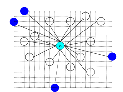
Figure 2. A representation of a mQAP sub-instance. The vertex $v_{s}$ and its $k$-nearest neighbors $knn(v_{s})$ induce a layout with available positions for the instance. The blue vertices are the lower and upper bounds of the induced layout.

3.5. Building mQAP instances for visualization

In this section, we propose a general method to compute flows and distances for the creation of the mQAP sub-instances to be optimized. However, we note that there is not a unique definition of flow between objects and distances between locations, so here we will present our choices for the visualization task given an initial layout of reference.

Creating sub-layouts – Given a sampled vertex $v_{s}\in G_{k-nn}$, let $p_{0}(v_{s})$ be its initial position in the layout produced by LargeVis. We denote the layout induced by a sampled vertex $v_{s}$ as $L(v_{s})$. Let $knn(v_{s})$ be its $k$-nearest neighbors. We generate each mQAP instance as follows. We first identify the initial positions where the neighbors are located in the layout (to find both the upper and lower bounds of the two coordinates of this group of objects). These correspond to the blue objects in Figure 2. Once the method identifies the bounds of this enclosing rectangle, we need to define the number of grid positions needed. We have chosen it to be a $50\times 50$ rectangular grid whose positions are separated by an equal distance based on the computed bounds (assuming that 2500 grid positions allow all objects to be allocated to a grid point).

Objective functions – A mQAP instance requires the definition of at least two types of flows between the data objects. In this work, we define two types of flows, the general structure of our approach would eventually handle other heuristic decisions.

The first definition of flows is motivated to deal with a problem that arises when working with datasets that might contain outliers, e.g., due to the corruption of the values or incorrect measurements. Intuitively, we want our visualization algorithms to lay objects organized as “islands”, groups of highly similar objects packed in nearby positions. Towards that end, we use a straightforward and low-cost estimation of density centered in a vertex in a layout. The $k^{*}$-core distance of a object $v$ in a layout, denoted as $c_{k^{*}}(v)$, corresponds to the Euclidean distance, in the layout, between $v$ and its $k^{*}$-th nearest neighbor. We also define the mutual reachability distance (Ester et al., 1996; Campello et al., 2013, 2015) between two vertices $v_{p}$, $v_{q}\in G_{k-nn}$ with parameter $k^{*}$ as:

(2) $$d_{k^{*}r}(v_{p},v_{q})=max\big{\{}c_{k^{*}}(v_{p}),~{}~{}c_{k^{*}}(v_{q}),~{}~{}d(p(v_{p}),p(v_{q}))\big{\}}.$$

Figure 3 shows how the mutual reachability distance is computed with three objects when $k^{*}=5$. First, for the blue object (located near the center of the figure) a circle encloses all objects which are its first five nearest neighbors. The same is the case for the larger green circle near the top with a different center and the red one near the bottom. Thus, the mutual reachability distance between blue and green is equal to the core distance of the green object. On the other hand, the mutual reachability distance from red to green corresponds to the distance from the center of the red circle to the center of the green one, since it is larger than both core distance.

Then, we define the first of the two flows for our mQAP instances as follows:

(3) $$\{f^{(1)}_{v_{p}v_{q}}\} =\Big{\{}\frac{1}{1+\exp(d_{k^{*}r}(v_{p},v_{q}))}\Big{\}},$$

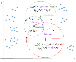
Figure 3. An example of mutual reachability distance computation with $k^{*}=5$.

where $d_{k^{*}r}(v_{p},v_{q})$ corresponds to the mutual reachability distance between $v_{p}$ and $v_{q}$.

For the second set of flows, we need some further definitions. Let $v_{p}$ and $v_{q}$ be two vertices belonging to the sub-layout $L(v_{s})$ and $d(p(v_{p}),p(v_{q}))$ the Euclidean distance between the positions assigned to these vertices in a layout. Let $p_{0}(v_{p})$ and $p_{0}(v_{q})$ be the positions assigned in the original layout provided by LargeVis. Let $d_{1}=d(p_{0}(v_{p}),p_{t}(v_{p}))$ and $d_{2}=d(p_{0}(v_{q}),p_{t}(v_{q}))$ correspond to the Euclidean distance between the initial position assigned to object $v_{p}$ and the one in which the same object is assigned after iteration $t$ of PasMoQAP. Also, $d_{x}=d(p_{0}(v_{p}),p_{0}(v_{q}))$ is the original Euclidean distance between $v_{p}$ and $v_{q}$ in the layout produced by LargeVis and $d_{y}=d_{t}(p(v_{p}),p_{t}(v_{q}))$ is their Euclidean distance on a layout $L_{t}$. We compute the second type of flow as follows:

(4) $$\{f^{(2)}_{v_{p}v_{q}}\} =\Big{\{}\frac{1}{(1+d(v_{p},v_{q}))}\Big{\}},$$

where $d(v_{p},v_{q})$ is the arithmetic average of these four distances $d(v_{p},v_{q})=(d_{1}+d_{2}+d_{x}+d_{y})/4$. We note, however, that this decision is non-standard as the flows depend on the actual position of the objects in a layout (i.e., in some sense “dynamically” changing during the optimization process). We expect that other flow definitions can also be explored in future contributions.

Positioning all the objects in the layout – mQAPViz keeps track of all the objects that have been allocated during the optimization process. However, it can happen that no all the objects are positioned after the optimization procedure. This case can happen because our algorithm uses the negative sampling method, selecting vertices and their $k$-nearest neighbors that will be allocated by the algorithm. In the best case scenario, the sampling technique will select all the objects in the dataset, but the technique cannot ensure it. In this case, for each not positioned vertex, our algorithm executes the optimization procedure (line 11 to 16 in Algorithm 1). In this way, we guarantee that all the objects are allocated via mQAPViz before generating the final visualizations.

3.6. Merging solutions from the Pareto fronts

mQAPViz computes many Pareto fronts, one for each vertex that was sampled using the negative sampling procedure. Each front contains several non-dominated solutions. Consequently, it is frequent that mQAPViz can assigns the same vertex to several available positions in the different layouts. However, in multi-objective optimization typically a user is interested in only a handful of solutions (from the front), which in our case correspond to different visualizations. We implement a simple method which merges solutions taken from the Pareto fronts. Thus, for each Pareto front, our heuristic procedure selects only three solutions (i.e., layouts) that are used to generate the final visualizations. Let $C^{(1)}$ and $C^{(2)}$ be the cost function which are computed using the flow definitions $f^{(1)}$ and $f^{(2)}$ respectively. Since we defined a bi-objective optimization problem, we can easily select two extreme solutions in a Pareto front according to the objectives $C^{(1)}$ and $C^{(2)}$ (Figure 4). We called these two solutions $L_{top}$ and $L_{bottom}$, and they represent the best solutions for objectives $C^{(1)}$ and $C^{(2)}$ respectively. The heuristic selects a third solution, which we called $L_{median}$, the one closest to the median ranked position of the solutions in the Pareto front after ordering. $L_{median}$ represents a “balanced” trade-off between both objectives functions. Then, for each computed Pareto front of the same type (e.g ‘top’, ‘bottom’ or ‘median’) (for each sampled vertex), and for each vertex that is not a seed vertex, we allocate it to one not yet allocated position (but assigned in at least one of these Pareto fronts). Due to the space restrictions, we only report the resulting visualizations obtained by merging by this process the $L_{median}$ layouts of each Pareto front.

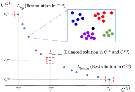
Figure 4. A representation of selecting of solutions to create the final visualizations. Our heuristic selects three visualizations (enclosed by squares) that belong to each Pareto front. The method chooses the best solution according to the cost $C^{(1)}$ ($L_{top}$), the best solution according to the cost $C^{(2)}$ ($L_{bottom}$), and a third solution that balances both objectives ($L_{median}$).

4. Experiments

In this section, we evaluate mQAPViz quantitatively and qualitatively on several real-life and large datasets. We implemented mQAPViz in C++ using the framework ParadisEO (Liefooghe et al., 2010). We performed the experiments on individual machines in The University of Newcastle’s Research Compute Grid that contains a cluster of 32 nodes Intel® Xeon® CPU E5-2698 v3 @ 2.30 GHz x 32 with 128 GB of RAM.

Table 1. A summary of the datasets’ statistics.

Dataset	# samples	# dimensions	# classes
Astroph	18,772	128	-
Pubmed	19,717	128	3
MNIST	70,000	784	10
Fashion-MNIST	70,000	784	10
Flickr	80,513	128	195
Pokec	1,632,803	128	-
Spammers	5,321,961	128	2

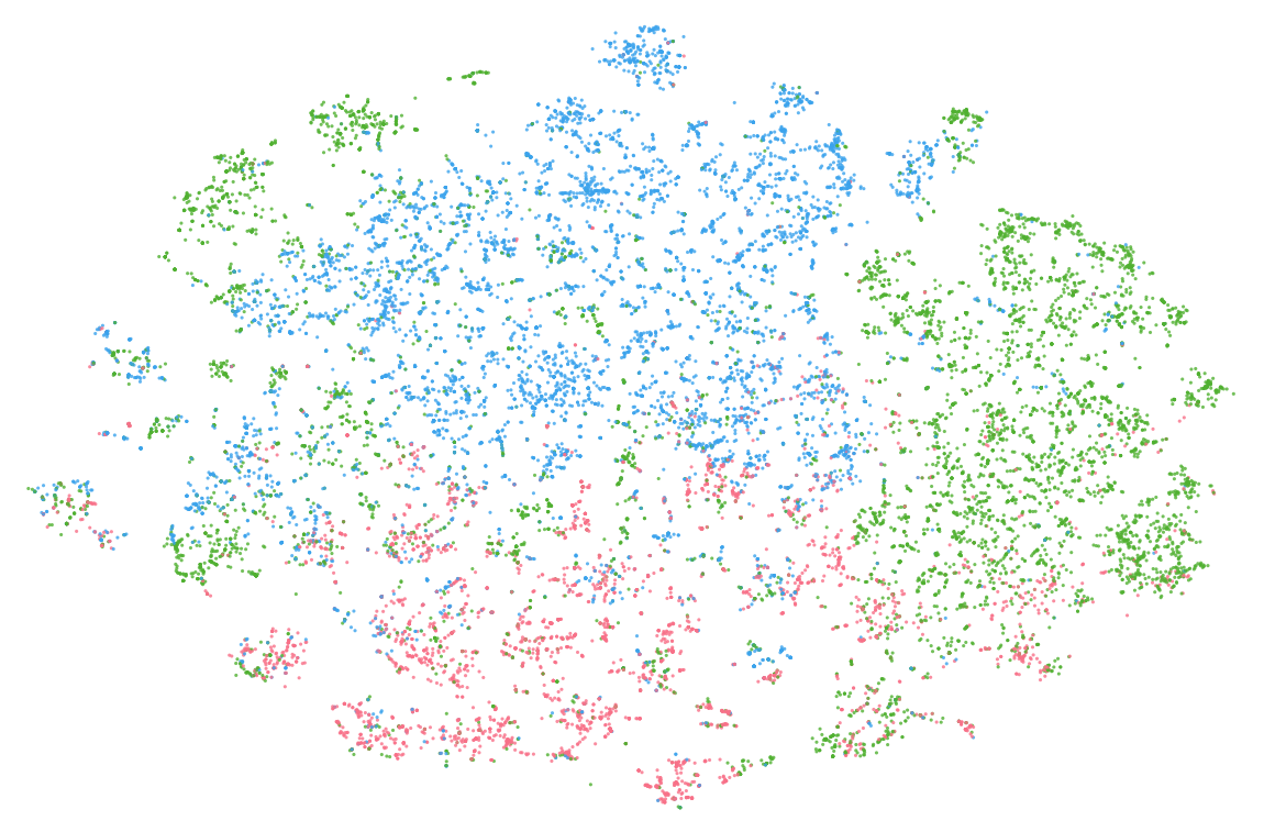
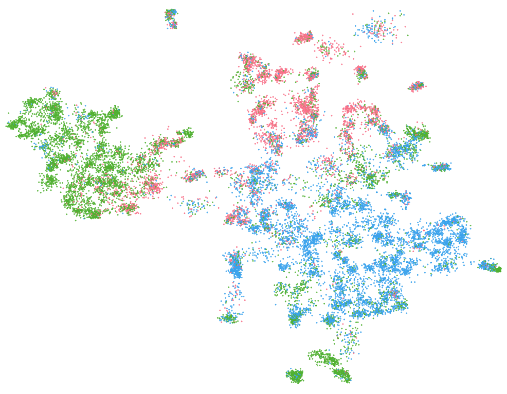
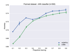
(a) Pubmed (t-SNE)	(b) Pubmed (mQAPViz)	(c) Pubmed (t-SNE vs. mQAPViz)
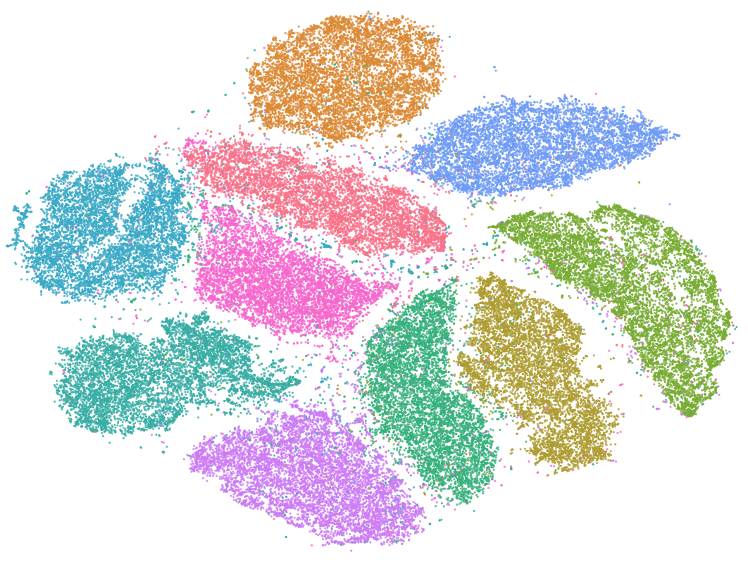
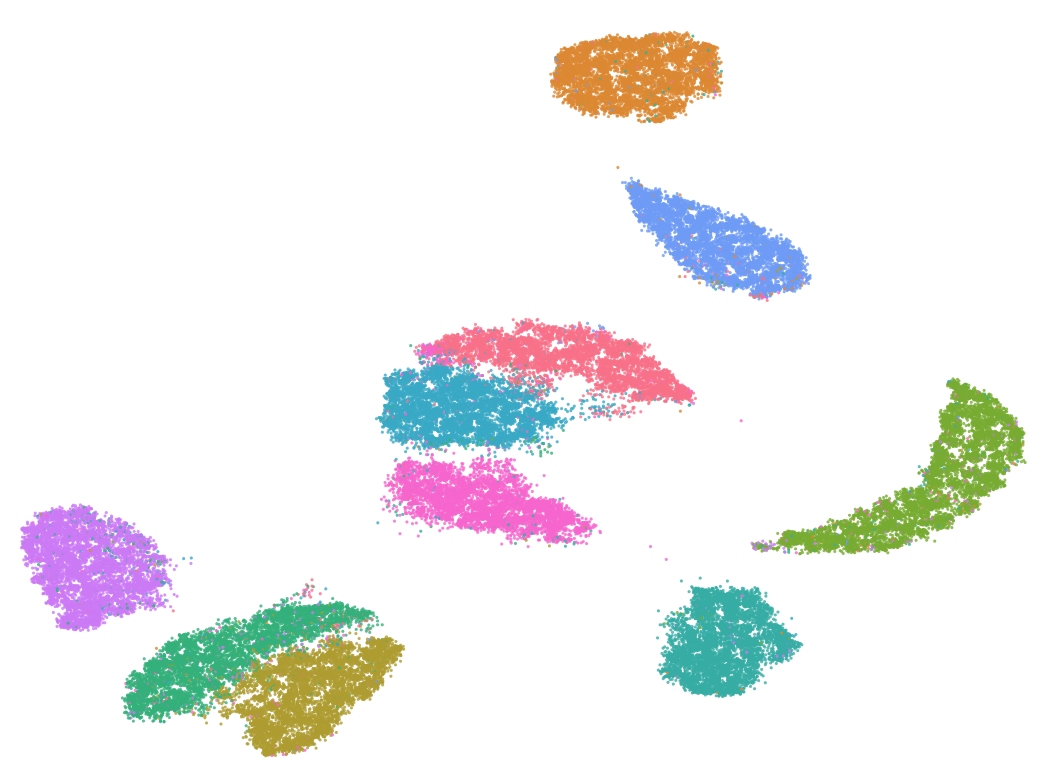
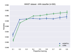
(d) MNIST (t-SNE)	(e) MNIST (mQAPViz)	(f) MNIST (t-SNE vs. mQAPViz)
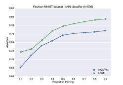
(g) Fashion-MNIST (t-SNE)	(h) Fashion-MNIST (mQAPViz)	(i) Fashion-MNIST (t-SNE vs. mQAPViz)
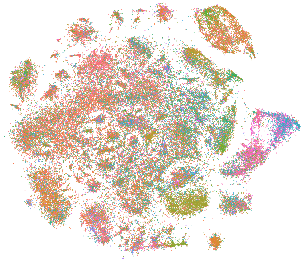
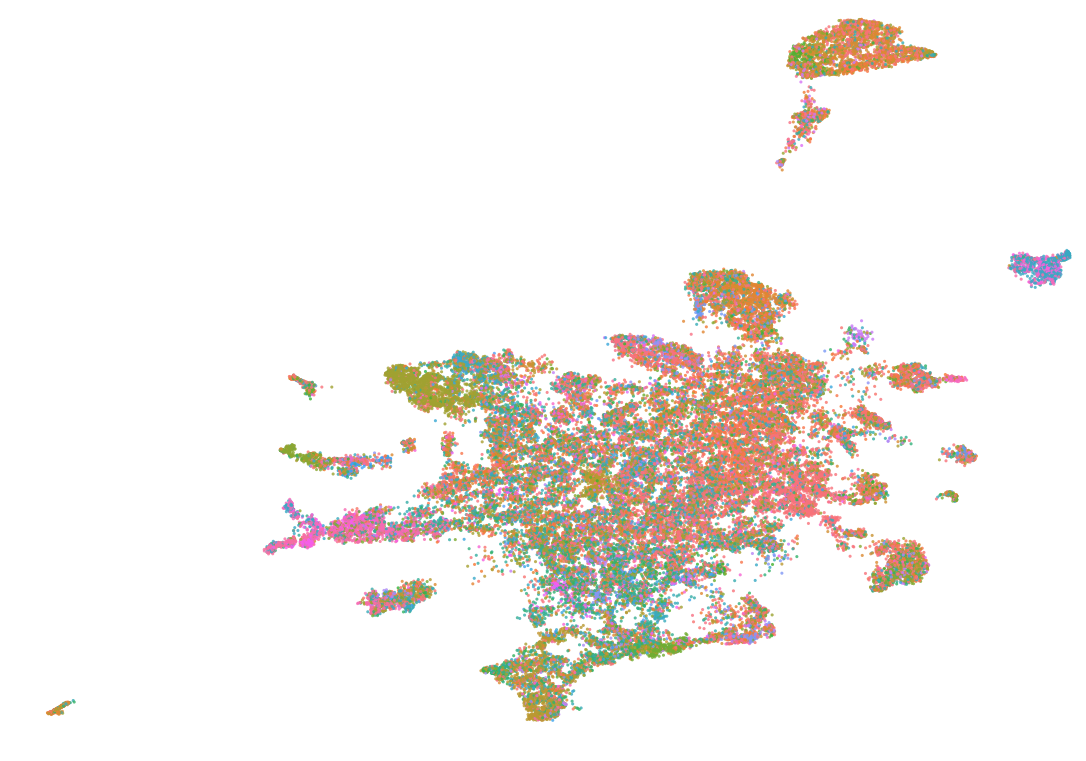
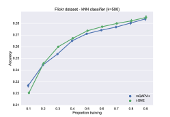
(j) Flickr (t-SNE)	(k) Flickr (mQAPViz)	(l) Flickr (t-SNE vs. mQAPViz)

Figure 5. Visualization of the datasets that contain true classes. Each color corresponds to a target class. We depict the visualizations obtained by t-SNE (column 1) and the visualizations obtained by mQAPViz (column 2). We also present the mean testing accuracy on different portions of training data. We executed 30 experiments on each training set, and we included the corresponding 95% confidence interval (column 3).

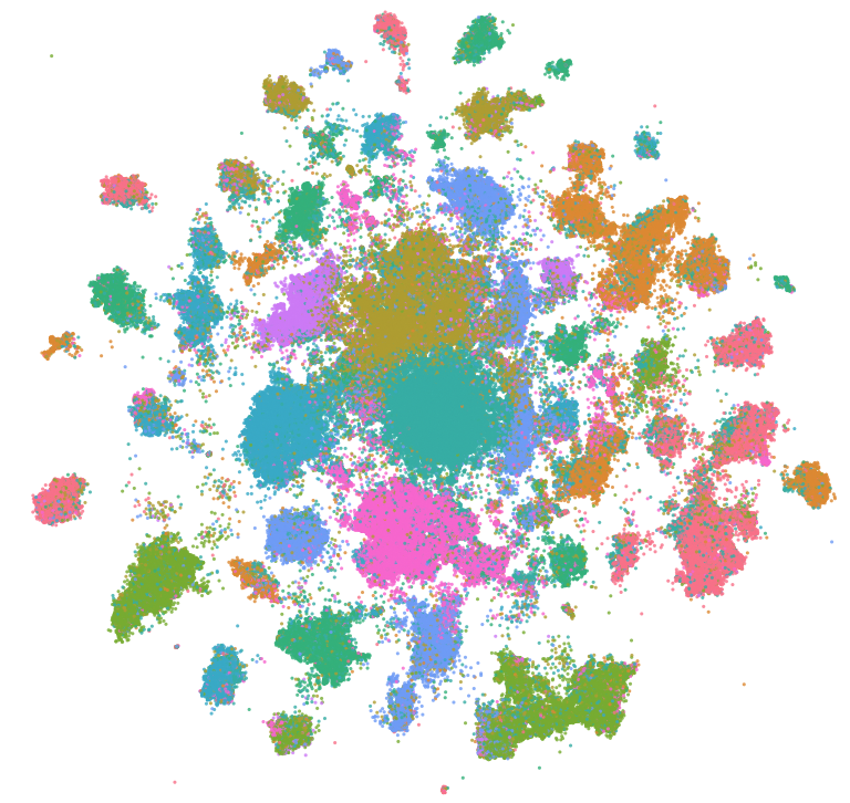
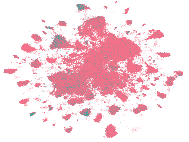
(a) Astroph (t-SNE)	(b) Astroph (mQAPViz)	(c) Pokec (mQAPViz)	(d) Spammers (mQAPViz)

Figure 6. Visualization computed using t-SNE and mQAPViz. In the Astroph visualizations depicted in (a) and (b), and the Pokec visualization (c) we use the K-means algorithm to obtain ten groups represented by the colors. In the case of the Spammers dataset (d), we use the original labels spammer (blue) and not spammer (red).

4.1. Datasets

We evaluate mQAPViz with multiple real-world and large-scale datasets (Table 1). In particular, we assess our method with the following datasets:

• Astroph: the Astro Physics collaboration network of authors who submitted papers to the Astro Physics category in arXiv. Each author is a data sample and an undirected edge corresponds to two authors that co-authored a publication.

• Pubmed: the diabetes scientific publication network. Each publication is a data sample and a directed edge represents that a publication cites another one.

• MNIST: the handwritten digits dataset in which each image is treated as a data object.

• Fashion-MNIST: the grayscale clothes dataset in which each image is treated as a data object.

• Flickr: the friendship network on Flickr. Each user is a data object and an undirected edge represent the friendship between two users.

• Pokec: the Slovakian social network dataset. Each user is a data object and an undirected edge represent the friendship between two users.

• Spammers: the anonymized spammers social network dataset. Each user is a data object which was manually labeled as spammer or not spammer. Given a user $u_{i}$ who performs an action targeting user $u_{j}$, a directed edge is created from $u_{i}$ to $u_{j}$.

Note that in the case of the network datasets, we first learn a feature vector representation for each node. Although DeepWalk (Perozzi et al., 2014) and node2vec (Grover and Leskovec, 2016) are two extremely efficient random walk-based representation learning algorithms, in our experiments we found that LINE (Tang et al., 2015) performs better on the particular visualization task. In consequence, we learn node representations through the LINE algorithm, and we represent each node by a vector of 128 dimensions, a value already proposed in the representation learning literature (Tang et al., 2015).

4.2. Evaluation

To evaluate mQAPViz, we compare our visualizations against the accelerated state-of-the-art approach for visualizing high dimensional data called t-SNE. We use the C++ Barnes-Hut t-SNE implementation published by the authors.

Model parameters and settings – For the model parameters in t-SNE, we set $\theta=0.5$, the number of iterations to 1,000, and the initial learning rate to 200 which are suggested in (Van Der Maaten, 2014). For both LINE and LargeVis, the size of mini-batches is set as 1; the learning rate is set as $\rho_{t}=\rho(1-t/T)$, where $T$ is the total number of edges samples or mini-batches. The initial learning rates used by LINE and LargeVis are $\rho_{0}=0.025$ and $\rho_{0}=1$ respectively. All these parameters are suggested by the authors of (Tang et al., 2016) (including setting the number of negative samples to 5 and the unified weight of the negative edges to 7). In mQAPViz, we compute the visualizations by sampling 30% of the nodes in the $G_{k-nn}$.

Quantitative evaluation – Assessing the quality of a visualization outcome is an inherently subjective task. To overcome this issue and to quantitatively evaluate the visualizations, we apply the $k$-NN classifier (implemented in scikit-learn) to classify the samples based on their visualization outcomes (i.e., 2D representation). The idea of this methodology is that a good visualization should be able to preserve the structure of the original data as much as possible and, therefore, a high classification accuracy would still be present even if just working with the low-dimensional representation. We report on the results of $k$-NN classifiers on different proportions of the training data (with $k=500$). For each proportion, we train the classifier thirty times on different training sets. To evaluate the performance of a classifier, we report the mean testing accuracy over the thirty rounds and the corresponding 95% confidence interval (column 3, Figure 5). We observe that in three out of four datasets, mQAPViz is at least competitive with respect to t-SNE. Fashion-MNIST is the only dataset in which we can see that t-SNE quantitatively outperforms mQAPViz.

Visualizations – We show several visualization examples to evaluate the quality of mQAPViz visualizations against t-SNE (Figure 5, columns 1 and 2). The colors correspond to the classes (Pubmed, MNIST, Fashion-MNIST, Flickr, and Spammers) or partitions computed with the K-means based on the high-dimensional representation (Astroph and Pokec, Figure 6) in which we partitioned the dataset in ten groups. We observe in the smallest dataset that the visualizations generated by both methods are meaningful and comparable to each other. On the larger datasets, we argue the visualizations generated by the mQAPViz are more intuitive. In the case of our larger datasets with 1.6M and 5.3M objects, t-SNE could not compute a visualization due to its high memory consumption. We can see in the Pokec visualization computed with mQAPViz (Figure 6c) several groups of objects that seem to share some common characteristics. In the case of the Spammer visualization (Figure 6d), we observe that spammer users are grouped in, at least, four different regions of the layout. With ad-hoc tools, we may isolate these lands of objects to perform further analyses.

5. Conclusions

In this study we proposed what is, to the best of our knowledge, the first method that uses a multi-objective optimization algorithm to compute visualizations of large datasets. mQAPViz is based on a divide-and-conquer approach in which several mQAP sub-instances are defined using the layout induced by sampled nodes and their nearest neighbors that belong to an efficiently computed k-NNG. Although we report results on a cluster grid, the method also allows us to generate visualizations of a million data objects in a single multi-core machine without requiring any special distributed processing architecture. Our experiments showed that mQAPViz is competitive against t-SNE using a simple quantitative evaluation. The visualizations generated with mQAPViz can later be used for further data analyses tasks.

We limited our study by evaluating two objective functions. However, the method could also accept other alternative objective functions, for example, considering both high- and low-dimensional data. Also, at this moment, our method can be used on data snapshots, excluding potential temporal associations between the objects. Thus, another challenging direction is to compute visualizations using multi-objective optimization to support the analysis of datasets that dynamically change across space and time (i.e., spatio-temporal datasets).

- (1)
- Abbiw-Jackson et al. (2006) Roselyn Abbiw-Jackson, Bruce L. Golden, S. Raghavan, and Edward Wasil. 2006. A divide-and-conquer local search heuristic for data visualization. Computers & OR 33, 11 (2006), 3070–3087.
- Belkin and Niyogi (2003) Mikhail Belkin and Partha Niyogi. 2003. Laplacian eigenmaps for dimensionality reduction and data representation. Neural computation 15, 6 (2003), 1373–1396.
- Bentley (1975) Jon Louis Bentley. 1975. Multidimensional binary search trees used for associative searching. Commun. ACM 18, 9 (1975), 509–517.
- Campello et al. (2013) Ricardo JGB Campello, Davoud Moulavi, and Jörg Sander. 2013. Density-based clustering based on hierarchical density estimates. In Pacific-Asia conference on knowledge discovery and data mining. Springer, 160–172.
- Campello et al. (2015) Ricardo JGB Campello, Davoud Moulavi, Arthur Zimek, and Jörg Sander. 2015. Hierarchical density estimates for data clustering, visualization, and outlier detection. ACM Transactions on Knowledge Discovery from Data (TKDD) 10, 1 (2015), 5.
- Clark et al. (2012) Michael B. Clark, Rebecca L. Johnston, Mario Inostroza-Ponta, Archa H. Fox, Ellen Fortini, Pablo Moscato, Marcel E. Dinger, and John S. Mattick. 2012. Genome-wide analysis of long noncoding RNA stability. Genome research 22, 5 (2012), 885–898.
- Deb (2001) Kalyanmoy Deb. 2001. Multi-objective optimization using evolutionary algorithms. Vol. 16. John Wiley & Sons.
- Ester et al. (1996) Martin Ester, Hans-Peter Kriegel, Jörg Sander, Xiaowei Xu, and others. 1996. A Density-Based Algorithm for Discovering Clusters in Large Spatial Databases with Noise. In Proceedings of the Second International Conference on Knowledge Discovery and Data Mining (KDD-96), Portland, Oregon, USA. 226–231.
- Few (2009) Stephen Few. 2009. Now you see it: simple visualization techniques for quantitative analysis. Analytics Press.
- Fruchterman and Reingold (1991) Thomas M. J. Fruchterman and Edward M. Reingold. 1991. Graph Drawing by Force-directed Placement. Software: Practice and Experience 21, 11 (1991), 1129–1164.
- Grover and Leskovec (2016) Aditya Grover and Jure Leskovec. 2016. node2vec: Scalable feature learning for networks. In Proceedings of the 22nd ACM SIGKDD International Conference on Knowledge Discovery and Data Mining. ACM, 855–864.
- Inostroza-Ponta et al. (2011) Mario Inostroza-Ponta, Regina Berretta, and Pablo Moscato. 2011. QAPgrid: A two level QAP-based approach for large-scale data analysis and visualization. PloS one 6, 1 (2011), e14468.
- Li and Kurata (2005) Weijiang Li and Hiroyuki Kurata. 2005. A grid layout algorithm for automatic drawing of biochemical networks. Bioinformatics 21, 9 (2005), 2036–2042.
- Liefooghe et al. (2010) Arnaud Liefooghe, Laetitia Jourdan, Thomas Legrand, Jérémie Humeau, and El-Ghazali Talbi. 2010. ParadisEO-MOEO: A Software Framework for Evolutionary Multi-Objective Optimization. In Advances in Multi-Objective Nature Inspired Computing. Studies in Computational Intelligence, Vol. 272. Springer, 87–117.
- Maaten and Hinton (2008) Laurens van der Maaten and Geoffrey Hinton. 2008. Visualizing data using t-SNE. Journal of Machine Learning Research 9, Nov (2008), 2579–2605.
- Mikolov et al. (2013) Tomas Mikolov, Ilya Sutskever, Kai Chen, Greg S Corrado, and Jeff Dean. 2013. Distributed representations of words and phrases and their compositionality. In Advances in neural information processing systems. 3111–3119.
- Perozzi et al. (2014) Bryan Perozzi, Rami Al-Rfou, and Steven Skiena. 2014. Deepwalk: Online learning of social representations. In Proceedings of the 20th ACM SIGKDD international conference on Knowledge discovery and data mining. ACM, 701–710.
- Roweis and Saul (2000) Sam T Roweis and Lawrence K Saul. 2000. Nonlinear dimensionality reduction by locally linear embedding. science 290, 5500 (2000), 2323–2326.
- Sanhueza et al. (2017) Claudio Sanhueza, Francia Jiménez, Regina Berretta, and Pablo Moscato. 2017. PasMoQAP: A parallel asynchronous memetic algorithm for solving the Multi-Objective Quadratic Assignment Problem. In 2017 IEEE Congress on Evolutionary Computation, CEC 2017, Donostia, San Sebastián, Spain, June 5-8, 2017. IEEE, 1103–1110.
- Tang et al. (2016) Jian Tang, Jingzhou Liu, Ming Zhang, and Qiaozhu Mei. 2016. Visualizing large-scale and high-dimensional data. In Proceedings of the 25th International Conference on World Wide Web. International World Wide Web Conferences Steering Committee, 287–297.
- Tang et al. (2015) Jian Tang, Meng Qu, Mingzhe Wang, Ming Zhang, Jun Yan, and Qiaozhu Mei. 2015. Line: Large-scale information network embedding. In Proceedings of the 24th International Conference on World Wide Web. ACM, 1067–1077.
- Tenenbaum et al. (2000) Joshua B. Tenenbaum, Vin De Silva, and John C. Langford. 2000. A global geometric framework for nonlinear dimensionality reduction. Science 290, 5500 (2000), 2319–2323.
- Van Der Maaten (2014) Laurens Van Der Maaten. 2014. Accelerating t-SNE using tree-based algorithms. Journal of machine learning research 15, 1 (2014), 3221–3245.
- Van Der Maaten et al. (2009) Laurens Van Der Maaten, Eric Postma, and Jaap Van den Herik. 2009. Dimensionality reduction: a comparative. J Mach Learn Res 10 (2009), 66–71.
- Warren et al. (2017) Chloe Warren, Mario Inostroza-Ponta, and Pablo Moscato. 2017. Using the QAPgrid Visualization Approach for Biomarker Identification of Cell-Specific Transcriptomic Signatures. Bioinformatics: Volume II: Structure, Function, and Applications (2017), 271–297.
- Zitzler and Thiele (1999) Eckart Zitzler and Lothar Thiele. 1999. Multiobjective evolutionary algorithms: a comparative case study and the strength Pareto approach. IEEE Trans. Evolutionary Computation 3, 4 (1999), 257–271.