0-Pierced Triangles within a Poisson Overlay

Abstract

Let the Euclidean plane be simultaneously and independently endowed with a Poisson point process and a Poisson line process, each of unit intensity.  Consider a triangle $T$ whose vertices all belong to the point process.  The triangle is 0-pierced if no member of the line process intersects any side of $T$.  Our starting point is Ambartzumian’s 1982 joint density for angles of $T$; our exposition is elementary and raises several unanswered questions.

A triangle with angles $\alpha$, $\beta$, $\gamma$ is acute if $\max\{\alpha,\beta,\gamma\}<\pi/2$ and well-conditioned if $\min\{\alpha,\beta,\gamma\}>\pi/6$.  Given a random mechanism for generating triangles in the plane, we dutifully calculate corresponding probabilities out of sheer habit and for the sake of numerical concreteness.

Beginning with a Poisson point process of unit intensity, let us form a triangle by taking the convex hull of three particles (members of the process).  The triangle is 0-filled if no other particles are contained in the convex hull.  Study of such configurations is complicated by the prevalence of long, narrow triangles with angles typically $\approx 0$ or $\approx\pi$.  We defer discussion of these until later.

Beginning with a Poisson point process and a Poisson line process, also of unit intensity and independent, let us form a triangle as before.  The triangle is 0-pierced if the intersection of each line with the convex hull is always empty.  Nothing is presumed about the existence or number of other interior particles; there may be $0$ or $1$ or $2$ or many more.  Since the angles satisfy $\alpha+\beta+\gamma=\pi$, we can eliminate $\gamma$ from consideration and write the joint density for $\alpha$, $\beta$ as [1, 2, 3, 4]

$$\frac{42}{\pi}\dfrac{\sin(x)\sin(y)\sin(x+y)}{\left[\sin(x)+\sin(y)+\sin(x+y)\right]^{4}}$$

where $x>0$, $y>0$, $x+y<\pi$. This is a remarkable result, owing to the scattered complexity of particles overlaid with lines. Integrating out $y$, we obtain the marginal density for $\alpha$:

$$f(x)=\frac{21}{2\pi}\frac{\left(7-5\cos(x)\right)\left(1+\cos(x)\right)+4\left(5-\cos(x)\right)\left(1-\cos(x)\right)\ln\left(\sin(\frac{x}{2})\right)}{\left(1+\cos(x)\right)^{4}}$$

and

$$\begin{array}[c]{ccc}\mathbb{E}(\alpha)=\dfrac{\pi}{3}=\,1.0471975511...,&&\mathbb{E}(\alpha^{2})=\dfrac{13}{10}-2\ln(2)+4\ln(2)^{2}=1.8355176945....\end{array}$$

Corresponding to the density for $\max\{\alpha,\beta,\gamma\}$, the expression $3f(x)$ holds when $\pi/2<x<\pi$; the expression when $\pi/3<x<\pi/2$ is $3\tilde{f}(x)$ where

$$\tilde{f}(x)=\frac{21}{2\pi}\frac{\left(7-4\cos(x)\right)\left(1-2\cos(x)\right)-4\left(5-\cos(x)\right)\left(1-\cos(x)\right)\ln\left(2\sin(\frac{x}{2})\right)}{\left(1+\cos(x)\right)^{4}}.$$

It thus follows that

$$\mathbb{P}(\text{a typical 0-pierced triangle is acute})=\frac{96-132\ln(2)-\pi}{2\pi}=0.2169249267....\text{ }$$

Corresponding to the density for $\min\{\alpha,\beta,\gamma\}$, the expression $-3\tilde{f}(x)$ holds when $0<x<\pi/3$ and hence

$$\begin{array}[c]{l}\mathbb{P}(\text{a typical 0-pierced triangle is well-conditioned})=\vskip 6.0pt plus 2.0pt minus 2.0pt\\ \dfrac{-3144+1584\sqrt{3}+(-2190+1338\sqrt{3})\ln(2)+(4380-2676\sqrt{3})\ln(-1+\sqrt{3})+(71+41\sqrt{3})\pi}{2(71+41\sqrt{3})\pi}\\ =0.2393922701....\end{array}$$

From $\mathbb{V}(\alpha+\beta+\gamma)=0$, we deduce that $\mathbb{E}(\alpha\beta)-\mathbb{E}(\alpha)\mathbb{E}(\beta)=-(1/2)\mathbb{V}(\alpha)$ and therefore

$$\mathbb{E}(\alpha\,\beta)=-\dfrac{13}{10}+\ln(2)-2\ln(2)^{2}+\frac{\pi^{2}}{6}=0.7271752195....$$

Simulation provides compelling evidence that Ambartzumian’s [1, 2] joint density is valid – see Figure 1 – although it does not provide insight leading to an actual proof.

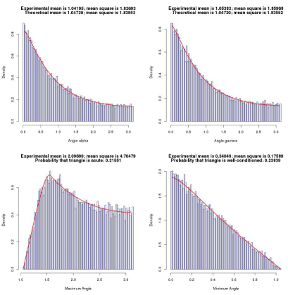
Figure 1: Histograms for angles, maximum angle and minimum angle in 0-pierced triangles.

1 Related Expressions

We turn attention to the bivariate densities

$$C_{j}\dfrac{\sin(x)\sin(y)\sin(x+y)}{\left[\sin(x)+\sin(y)+\sin(x+y)\right]^{j}}$$

where $x>0$, $y>0$, $x+y<\pi$ and

$$\begin{array}[c]{ccccc}C_{1}=\dfrac{4}{12-\pi^{2}},&&C_{2}=\dfrac{1}{\left(-2+3\ln(2)\right)\pi},&&C_{3}=8.\end{array}$$

The case $j=1$ appears in [5, 6] with regard to cells of a Goudsmit-Miles tessellation (sampled until a triangle emerges); the case $j=3$ appears in [7, 8] with regard to triangles created via breaking a line segment (in two places at random).  For $j=2$, we obtain the univariate density for $\alpha$:

$$g(x)=\dfrac{1}{2\left(-2+3\ln(2)\right)\pi}\frac{\left(\pi-x\right)\sin(x)+4\left(1-\cos(x)\right)\ln\left(\sin(\frac{x}{2})\right)}{1+\cos(x)}$$

and

$$\mathbb{E}(\alpha^{2})=\dfrac{4\left(\pi^{2}-12\ln(2)\right)\ln(2)-3\zeta(3)}{6\left(-2+3\ln(2)\right)}=1.4611131303...$$

where $\zeta(3)$ is Apéry’s constant [9].

Corresponding to the density for $\max\{\alpha,\beta,\gamma\}$, the expression $3g(x)$ holds when $\pi/2<x<\pi$; the expression when $\pi/3<x<\pi/2$ is $3\tilde{g}(x)$ where

$$\tilde{g}(x)=\dfrac{1}{2\left(-2+3\ln(2)\right)\pi}\frac{\left(3x-\pi\right)\sin(x)-4\left(1-\cos(x)\right)\ln\left(2\sin(\frac{x}{2})\right)}{1+\cos(x)}.$$

It thus follows that

$$\mathbb{P}(\text{a typical such triangle is acute}) =\frac{-24\ln(2)+\left(4-3\ln(2)\right)\pi+12G}{4\left(-2+3\ln(2)\right)\pi}$$

$$=0.3903338870...$$

and $G$ is Catalan’s constant [10].  Corresponding to the density for $\min\{\alpha,\beta,\gamma\}$, the expression $-3\tilde{g}(x)$ holds when $0<x<\pi/3$ and hence

$$\begin{array}[c]{l}\mathbb{P}(\text{a typical such triangle is well-conditioned})=0.4190489201...\end{array}$$

(exact expression omitted for reasons of length).  As before, we deduce that

$$\mathbb{E}(\alpha\,\beta)=\dfrac{2\left(\pi^{2}+24\ln(2)\right)\ln(2)-4\pi^{2}+3\zeta(3)}{12\left(-2+3\ln(2)\right)}=0.9143775016....$$

What’s missing, of course, is a natural procedure for generating (not necessarily planar) triangles whose angles $\alpha$, $\beta$, $\gamma$ obey the distributional law prescribed by $j=2$.

2 0-Filled Triangles

The phrase “0-filled” first appeared in [11, 12].  Let us initially discuss the simulation underlying 0-pierced triangles.  Given a parameter value $\lambda>0$, we generated data $(\alpha_{1},\beta_{1})$, $(\alpha_{2},\beta_{2})$, …, $(\alpha_{n},\beta_{n})$ via Poisson overlays in the planar disk of radius $\lambda$ centered at the origin. Our goal was to verify a probability theoretic expression:

$$\mathbb{P}(x<\alpha\leq x+dx,\;y<\beta\leq y+dy)=\frac{42}{\pi}\dfrac{\sin(x)\sin(y)\sin(x+y)}{\left[\sin(x)+\sin(y)+\sin(x+y)\right]^{4}}\,dx\,dy$$

as $\lambda\rightarrow\infty$.  This was done simply by histogramming the data, given large enough $n$ and $\lambda$.

For 0-filled triangles, however, we face a situation where the goal is less tangible.  Ambartzumian’s measure theoretic expression [2]:

$$\mathbb{M}(x<\alpha\leq x+dx,\;y<\beta\leq y+dy)=\dfrac{2}{\sin(x)\sin(y)\sin(x+y)}\,dx\,dy$$

cannot be normalized to give a probability density (that is, encompassing unit area).  It follows that [13, 14]

$$\mathbb{M}(x<\max\{\alpha,\beta,\gamma\}\leq x+dx)=\left\{\begin{array}[c]{lll}-12\csc(x)^{2}\ln\left(2\cos(x)\right)&&\text{if }\pi/3\leq x<\pi/2,\\ \infty&&\text{if }\pi/2\leq x<\pi\end{array}\right.$$

and, for $0<x<\pi/3$,

$$\mathbb{M}(x<\min\{\alpha,\beta,\gamma\}\leq x+dx)=12\csc(x)^{2}\ln\left(2\cos(x)\right)$$

– see Figures 2 and 3 – but verification is problematic.

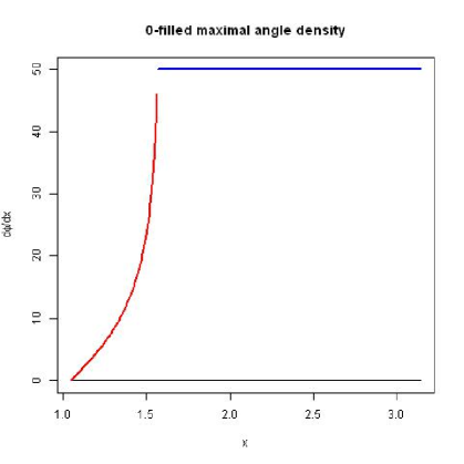
Figure 2: $\phi(x)=4\left(3x-\pi+3\cot(x)\ln(2\cos(x))\right)$ for $\pi/3<x<\pi/2$.

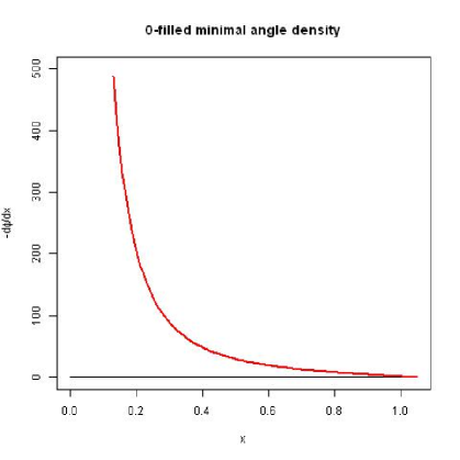
Figure 3: $\phi(x)=4\left(3x-\pi+3\cot(x)\ln(2\cos(x))\right)$ for $0<x<\pi/3$.

As before, we can generate data over disks of increasing radius $\lambda$.  Figure 4 provides histograms of $\alpha$ for $\lambda=2,3,4,5$; Figures 5 and 6 do likewise for $\max\{\alpha,\beta,\gamma\}$ and $\min\{\alpha,\beta,\gamma\}$.  Clearly

$$\lim_{\lambda\rightarrow\infty}\mathbb{P}(\text{a typical 0-filled triangle is acute})=0,$$

$$\lim_{\lambda\rightarrow\infty}\mathbb{P}(\text{a typical 0-filled triangle is well-conditioned})=0$$

on empirical grounds.  Unfortunately we do not know how to confirm theoretical predictions stemming from [13, 14]:

$$\mathbb{M}(\text{a typical 0-filled triangle is acute})=2\pi\approx 6.283,$$

$$\mathbb{M}(\text{a typical 0-filled triangle is well-conditioned})=2\left(3\sqrt{3}\ln(3)-\pi\right)\approx 5.134$$

via our experimental simulation.  A procedure to adjust the histogramming of the data, in order to demonstrate an improved fit as $\lambda\rightarrow\infty$, would be welcome.

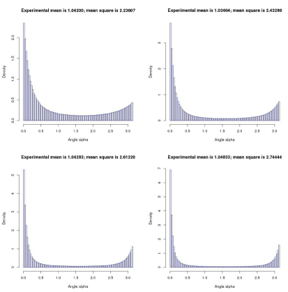
Figure 4: Histograms for arbitrary angle in 0-filled triangles, for increasing $\lambda$.

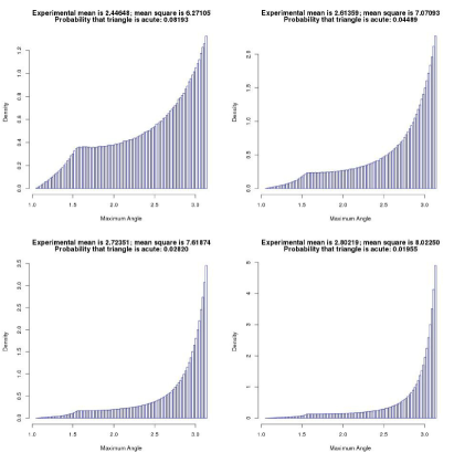
Figure 5: Histograms for maximum angle in 0-filled triangles, for increasing $\lambda$.

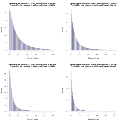
Figure 6: Histograms for minimum angle in 0-filled triangles, for increasing $\lambda$.

3 Process Intensities

We report here on work in [15].  Given a Poisson overlay $\Omega$, define a $\mathbf{T}_{\cdot 0}$ process to be the set of all 0-pierced triangles within $\Omega$.  Let the intensity $i$ of the process be the mean number of triangles per unit area.  It is known that

$$i(T_{\cdot 0})=\frac{2\pi^{2}}{21}=0.9399623239...=\frac{1}{6}(5.6397739434...).$$

The factor of $1/6$ arises because the three vertices were (apparently) ordered in [15], thus every triangle was counted $3!=6$ times.  We may similarly examine the set of all 0-filled triangles; it is not surprising that $i(T_{0\cdot})=\infty$.  Most interesting, however, is the set of all triangles that are both 0-filled and 0-pierced:

$$i(T_{00}) =0.6554010386...=\frac{1}{6}(3.9324062319...)$$

$$=\frac{\pi}{18\sqrt{3}}{\displaystyle\int\limits_{0}^{\pi}}\frac{\xi(x)\eta(x)}{\sqrt{b(x)\left(a(x)-c(x)\right)}}\sin\left(\frac{x}{2}\right)dx$$

where

$$\begin{array}[c]{ccccc}a(x)=\dfrac{2}{3}\left(\cos\left(\dfrac{x}{3}\right)+1\right),&&b(x)=\dfrac{2}{3}\left(\cos\left(\dfrac{x-2\pi}{3}\right)+1\right),&&c(x)=\dfrac{2}{3}\left(\cos\left(\dfrac{x+2\pi}{3}\right)+1\right),\end{array}$$

$$\begin{array}[c]{ccc}q(x)=\sqrt{\dfrac{a(x)\left(b(x)-c(x)\right)}{b(x)\left(a(x)-c(x)\right)}},&&h(x)=2(27)^{1/4}\cos\left(\dfrac{x}{2}\right)^{-1/2},\end{array}$$

$$\xi(x)=2\left(4+h(x)^{2}\right)-\sqrt{\pi}\left(6+h(x)^{2}\right)h(x)\exp\left(\frac{h(x)^{2}}{4}\right)\operatorname*{erfc}\left(\frac{h(x)}{2}\right),$$

$$\eta(x)=\left(\frac{3}{c(x)}-\frac{3}{a(x)}\right)E(q(x))+\left(\frac{3}{a(x)}-1\right)K(q(x));$$

$$\begin{array}[c]{ccc}K(y)={\displaystyle\int\limits_{0}^{\pi/2}}\dfrac{1}{\sqrt{1-y^{2}\sin(\theta)^{2}}}\,d\theta,&&E(y)={\displaystyle\int\limits_{0}^{\pi/2}}\sqrt{1-y^{2}\sin(\theta)^{2}}\,d\theta\end{array}$$

are complete elliptic integrals of the first and second kind; and

$$\operatorname*{erf}(z)=\frac{2}{\sqrt{\pi}}{\displaystyle\int\limits_{0}^{z}}\exp(-\tau^{2})\,d\tau=1-\operatorname*{erfc}\left(z\right)$$

is the error function.  Formulas (7) and (8) in [15], devoted to a more general scenario $T_{k\ell}$ than our $T_{00}$, specialize to

$${\displaystyle\int\limits_{0}^{\infty}}s\exp\left(-s-t\sqrt{s}\right)\,ds=\frac{1}{8}\left[2\left(4+t^{2}\right)-\sqrt{\pi}\left(6+t^{2}\right)t\exp\left(\frac{t^{2}}{4}\right)\operatorname*{erfc}\left(\frac{t}{2}\right)\right]$$

for $t>0$ (avoiding use of a parabolic cylinder function $D_{-4}\left(t/\sqrt{2}\right)$ which is less familiar).

Theory fails for $T_{00}$ – we do not possess density predictions for the histograms in Figure 7 – nor do we know exact probabilities that a such a triangle is acute or well-conditioned.

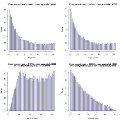
Figure 7: Histograms for angles, maximum angle and minimum angle in $T_{00}$ triangles.

References

[1]R. V. Ambartzumian, Random shapes by factorization,
Statistics in Theory and Practise, Essays in Honour of Bertil
Matérn, ed. B. Ranneby, Swedish University of Agricultural Sciences,
Section of Forest Biometry, 1982, pp. 35-41; MR0688997 (84c:62004).
[2]R. V. Ambartzumian, Factorization in integral and
stochastic geometry, Stochastic Geometry, Geometric Statistics,
Stereology, Proc. 1983 Oberwolfach conf., ed. R. Ambartzumian and W. Weil,
Teubner, 1984, pp. 14–33; MR0794864.
[3]D. G. Kendall, Shape manifolds, Procrustean metrics, and
complex projective spaces, Bull. London Math. Soc. 16 (1984) 81–121;
MR0737237 (86g:52010).
[4]V. K. Oganyan, On triangle shapes formed by points of a
Poisson process in the plane (in Russian), Akad. Nauk Armyan. SSR
Dokl., v. 81 (1985) n. 2, 59–63; MR0826342 (87h:60032).
[5]R. E. Miles, The various aggregates of random polygons
determined by random lines in a plane, Adv. Math. 10 (1973) 256–290;
MR0319232 (47 #7777).
[6]S. R. Finch, Random triangles V, Mathematical
Constants II, Cambridge Univ. Press, 2019, pp. 700–713; MR3887550.
[7]S. R. Finch, Uniform triangles with equality constraints, arXiv:1411.5216.
[8]S. R. Finch, Random triangles VI, Mathematical
Constants II, Cambridge Univ. Press, 2019, pp. 713–718; MR3887550.
[9]S. R. Finch, Apéry’s constant, Mathematical
Constants, Cambridge Univ. Press, 2003, pp. 40–53; MR2003519 (2004i:00001).
[10]S. R. Finch, Catalan’s constant, Mathematical
Constants, Cambridge Univ. Press, 2003, pp. 53–59; MR2003519 (2004i:00001).
[11]R. E. Miles, On the homogeneous planar Poisson point
process, Math. Biosci. 6 (1970) 85–127; MR0279853 (43 #5574).
[12]R. Cowan, A more comprehensive complementary theorem for
the analysis of Poisson point processes, Adv. Appl. Probab. 38 (2006)
581–601; MR2256870 (2007k:60138).
[13]H. S. Sukiasian, Two results on triangle shapes,
Stochastic Geometry, Geometric Statistics, Stereology, Proc. 1983
Oberwolfach conf., ed. R. Ambartzumian and W. Weil, Teubner, 1984, pp.
210–221; MR0794883.
[14]R. V. Ambartzumian, Factorization Calculus and
Geometric Probability, Cambridge Univ. Press, 1990, pp. 61–67; 158–160;
MR1075011 (92b:60013).
[15]V. R. Fatalov, Intensities of thinned processes of
triangles that are generated by a Poisson point process on the plane (in
Russian), Izv. Akad. Nauk Armyan. SSR Ser. Mat., v. 25 (1990) n. 4,
344–352, 413; Engl. transl. in Soviet J. Contemp. Math. Anal., v. 25
(1990) n. 4, 32–40; MR1115778 (92h:60018).