Atomic switch for control of heat transfer in coupled cavities

Abstract

Controlled heat transfer and thermal rectification in a system of two coupled cavities connected to thermal reservoirs are discussed. Embedding a dispersively interacting two-level atom in one of the cavities allows switching from a thermally conducting to resisting behavior. By properly tuning the atomic state and system-reservoir parameters, direction of current can be reversed. It is shown that a large thermal rectification is achievable in this system by tuning the cavity-reservoir and cavity-atom couplings. Partial recovery of diffusive heat transport in an array of $N$ cavities containing one dispersively coupled atom is discussed.

I Introduction

Coherent and controlled transfer of photons is of fundamental interest in quantum information processing and communication Northup and Blatt (2014). Recent developments in fabrication of suitably coupled cavities have made it possible to study their use in transferring information using photons as the carrier Meher et al. (2017); Zhong (2016); Yang et al. (2013). Highly tunable cavity couplings and resonance frequencies of coupled cavities make them suitable for photon transfer, quantum state transfer, entanglement generation, etc Majumdar et al. (2012); Almeida et al. (2016); Biella et al. (2015); Liu and Zhou (2015); Liao et al. (2010); Liew and Savona (2012). Transport of photons in an array can be modified by embedding atoms or Kerr-medium in the cavities which modify the cavity resonance frequencies Imamoḡlu et al. (1997); Felicetti et al. (2014); Qin and Nori (2016); Zhou et al. (2008); Brune et al. (1996). This helps to realize phenomenon such as photon blockade Imamoḡlu et al. (1997), quantum state switching Meher et al. (2017), generation of cat states Brune et al. (1992), localization and delocalization Schmidt et al. (2010); Meher and Sivakumar (2016), etc.

In the ideal case of a cavity being completely isolated from its surroundings, its dynamics is unitary. However, complete isolation of a system is not feasible. In this case, the evolution is not unitary. Simplest of this situation corresponds to coupling the system to a reservoir at zero absolute temperature. On incorporating such a reservoir, many of the photon transport phenomena indicated previously can be explained. However, the dynamics differs if the cavities are coupled to heat reservoirs at non-zero temperatures, where cavities exchange energy with reservoirs. In this context, coupled cavities can be used to transport energy between the thermal reservoirs Manzano and Kyoseva (2016); Xuereb et al. (2015). For a conventional bulk material, steady state heat transport is governed by

$$\textbf{J}=-\kappa\nabla T,$$ (1)

which is the Fourier’s law of heat conduction. Here J is the thermal current and $\nabla T$ is the temperature gradient. The proportionality constant $\kappa$ is the thermal conductivity, which is positive for all known materials. This law is valid if the system is close to its equilibrium, in which case linear response theory is applicable Garrido et al. (2001); Dhar (2008); Saito (2003); Michel et al. (2005); Dubi and Di Ventra (2009). Transport of heat by magnetic excitations in spin chains Saito et al. (1996); Landi et al. (2014); Schachenmayer et al. (2015); Werlang and Valente (2015); Manzano et al. (2012), phonons in atomic lattices Thingna et al. (2012); He et al. (2016), photons in cavity arrays Manzano and Kyoseva (2016); Asadian et al. (2013); Purkayastha et al. (2016a), etc. have been investigated. Similar to electronic devices, several thermal devices such as thermal diodes Li et al. (2004), thermal transistors Li et al. (2006), thermal ratchet Li et al. (2008), thermal logic gates Wang and Li (2007), thermal memory Wang and Li (2008), etc. based on non-equilibrium dynamics have been proposed.

A system away from equilibrium may violate the Fourier’s empirical law. There is no universal theory of heat transfer applicable to all nonequilibrium systems. A chain of coupled oscillators is known to violate the Fourier’s law of heat conduction in the sense that the thermal current is independent of system size and the heat transport is ballistic Rieder et al. (1967); Dhar (2008); Asadian et al. (2013); Zotos et al. (1997). Diffusive transport can be recovered by including anharmonicity or dephasing Hu et al. (1998); Debnath et al. (2017); Asadian et al. (2013); Shah and Gajjar (2013). The dynamics of nonequilibrium systems is conceptually rich with many unsolved problems.

Another interesting phenomenon is thermal rectification, which is essential for realizing thermal diodes and transistors Starr (1936); Li et al. (2004). A system shows thermal rectification if it possesses structural asymmetry allowing higher thermal current in one direction. Thermal rectification is known in the case of nanotubes Chang et al. (2006), quantum spin chains Zhang et al. (2009); Yan et al. (2009); Werlang et al. (2014), nonlinear oscillators Terraneo et al. (2002), two-level systems Segal and Nitzan (2005), etc.

In the present work, heat transfer in a system of two coupled cavities containing a single atom is discussed. The system-reservoir interaction is assumed to be of Lindblad type Lindblad (1976). Magnitude as well as direction of current can be controlled by suitably choosing the atomic state and the system-reservoir parameters. The system exhibits large thermal rectification for proper choices of the cavity-reservoir and cavity-atom couplings.

The present paper is organized as follows. In Sec. II, details of the system and its theoretical model are discussed to arrive at an expression for heat current. Also, various special cases of importance are indicated. Based on the dependence of the current on the reservoir temperatures and coupling parameters, violation of Fourier’s law is estabslished Sec. III. Thermal rectification behavior of the system is explored in Sec. IV. Generalization to $N$ cavities is discussed in Sec. V. Results are summarized in Sec. VI.

II Current in coupled cavities

A system of two linearly coupled cavities is described by the HamiltonianAgarwal (2012),

$$H_{1}= \omega_{L}a^{\dagger}_{L}a_{L}+\omega_{R}a^{\dagger}_{R}a_{R}+J(a_{L}^{\dagger}a_{R}+a_{L}a_{R}^{\dagger}),$$ (2)

where $\omega_{L}$ and $\omega_{R}$ are the resonance frequencies. The coupling strength between the cavities is $J$. In addition, a two-level atom is dispersively coupled to the right cavity and the corresponding atom-cavity interaction is governed by the Hamiltonian Gerry (1996),

$$H_{2}= \frac{\omega_{0}}{2}\sigma_{z}+\chi(\sigma_{+}\sigma_{-}+a^{\dagger}_{R}a_{R}\sigma_{z}),$$ (3)

where $\chi=g^{2}/(\omega_{0}-\omega_{R})$ is assumed to be positive. The states $\ket{e}$ and $\ket{g}$ are respectively the excited and ground states of the two-level atom. The operators $\sigma_{+}=\ket{e}\bra{g}$ and $\sigma_{-}=\ket{g}\bra{e}$ are the raising and lowering operators for the atom respectively. The energy operator for the atom is $\sigma_{z}=\ket{e}\bra{e}-\ket{g}\bra{g}$. The coupling strength between the atom and the cavity field is $g$ and the atomic transition frequency is $\omega_{0}$. This is an effective interaction obtained from Jaynes-Cummings model, if the atom and the cavity are highly detuned so that $\Delta=(\omega_{0}-\omega_{R})>>g$ and the mean number of photons $n$ is smaller than $\Delta^{2}/g^{2}$ Gerry (1996); Holland et al. (1991). Dispersive coupling between atom and cavity has been used to realize the cat states of the cavity field Brune et al. (1996, 1992).

The system considered in this work is a pair of linearly coupled cavities and a dispersively interacting atom in one of the cavities. Based on the discussion given above, the total Hamiltonian is

$$H=H_{1}+H_{2}= \frac{\omega_{0}}{2}\sigma_{z}+\omega_{L}a^{\dagger}_{L}a_{L}+\omega_{R}a^{\dagger}_{R}a_{R}+\chi(\sigma_{+}\sigma_{-}+a^{\dagger}_{R}a_{R}\sigma_{z})+J(a_{L}^{\dagger}a_{R}+a_{L}a_{R}^{\dagger}).$$ (4)

This Hamiltonian conserves the respective total excitation numbers for the cavity fields and the atom in the absence of dissipation, i.e., $[a_{L}^{\dagger}a_{L}+a_{R}^{\dagger}a_{R},H]=0$ and $[\sigma_{z},H]=0$. As a consequence, the atom and the field cannot exchange energy in the dispersive limit Brune et al. (1996).

The system is coupled to two reservoirs, each modelled as a collection of independent oscillators Carmichael (1999). The reservoir Hamiltonian is taken to be

$$H_{x}=\sum_{j}\omega_{xj}b_{xj}^{\dagger}b_{xj},$$

where $x=L$, $R$ is the index referring to the left reservoir and the right reservoir respectively. The creation and annihilation operators of the reservoirs obey the bosonic commutation relation $[b_{xj},b^{\dagger}_{xk}]=\delta_{jk}$. The arrangement of the cavities and reservoirs is shown in Fig. 1. The interaction Hamiltonian for the cavity-reservoir component is

$$H_{I}=\left(\sum_{j}g_{Lj}\right. (a_{L}^{\dagger}+a_{L})(b_{Lj}+b_{Lj}^{\dagger})$$

$$\left.+\sum_{j}g_{Rj}(a_{R}^{\dagger}+a_{R})(b_{Rj}+b_{Rj}^{\dagger})\right),$$

where $g_{Lj}(g_{Rj})$ is the coupling strength of left (right) cavity to $j$th mode of left (right) reservoir.

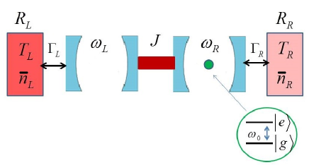
Figure 1: Schematic representation of system of coupled cavities with a two-level atom embedded in the right cavity. Both the cavities are also coupled with their respective reservoirs.

Under the Born-Markov and rotating wave approximations Gardiner and Zoller (2004); Diehl et al. (2008), the reduced joint density matrix for the two cavities (traced over the reservoirs) obeys Carmichael (1999)

$$\frac{\partial\rho}{\partial t}=-i[H,\rho]+\mathcal{D}_{L}(\rho)+\mathcal{D}_{R}(\rho),$$ (5)

where the Lindblad operators

$$\mathcal{D}_{x}(\rho)= \frac{\Gamma_{x}(\bar{n}_{x}+1)}{2}(2a_{x}\rho a_{x}^{\dagger}-a_{x}^{\dagger}a_{x}\rho-\rho a_{x}^{\dagger}a_{x})$$

$$+\frac{\Gamma_{x}\bar{n}_{x}}{2}(2a_{x}^{\dagger}\rho a_{x}-a_{x}a_{x}^{\dagger}\rho-\rho a_{x}a_{x}^{\dagger}),$$ (6)

for $x=L,R$. The parameters $\Gamma_{L}$ and $\Gamma_{R}$ are related to the coupling strengths as Biehs and Agarwal (2013)

$$\Gamma_{x}=2\pi\sum_{j}g_{xj}^{2}\delta(\omega_{xj}-\omega_{x}).$$ (7)

The two terms in Eqn. II correspond to energy flow from the system to the reservoir and vice-versa respectively. The dynamics generated by the master equation approach satisfies the detailed balance condition and gives the correct steady state if the different components of the system are weakly coupled Rivas et al. (2010); Purkayastha et al. (2016b); Manzano et al. (2012); Santos and Landi (2016).

The reservoirs $R_{L}$ and $R_{R}$ are assumed to be in thermal equilibrium at temperatures $T_{L}$ and $T_{R}$ respectively. The density operators which characterize the states of the reservoirs are

$$\varrho_{x}=\frac{e^{-H_{x}/k_{B}T_{x}}}{\text{Tr}\left(e^{-H_{x}/k_{B}T_{x}}\right)},$$ (8)

with mean photon numbers

$$\bar{n}_{x}=\frac{1}{\exp{(\omega_{x}/k_{B}T_{x})}-1},$$ (9)

where $x=L,R$.

The dynamics of the system can be understood from the temporal evolution of expectation values of various operators. The expectation values satisfy

$$\frac{d}{dt}\langle a_{L}^{\dagger}a_{L}\rangle=iJ(\langle a_{L}a_{R}^{\dagger}\rangle-\langle a_{L}^{\dagger}a_{R}\rangle)-\Gamma_{L}\langle a_{L}^{\dagger}a_{L}\rangle+\Gamma_{L}\bar{n}_{L},$$ (10a)

$$\frac{d}{dt}\langle a_{R}^{\dagger}a_{R}\rangle=-iJ(\langle a_{L}a_{R}^{\dagger}\rangle-\langle a_{L}^{\dagger}a_{R}\rangle)-\Gamma_{R}\langle a_{R}^{\dagger}a_{R}\rangle+\Gamma_{R}\bar{n}_{R},$$ (10b)

$$\frac{d}{dt}\langle a_{L}^{\dagger}a_{R}\rangle=i\Delta_{c}\langle a_{L}^{\dagger}a_{R}\rangle-iJ(\langle a_{L}^{\dagger}a_{L}\rangle-\langle a_{R}^{\dagger}a_{R}\rangle)-i\chi\langle a_{L}^{\dagger}a_{R}\sigma_{z}\rangle-\gamma\langle a_{L}^{\dagger}a_{R}\rangle,$$ (10c)

$$\frac{d}{dt}\langle a_{L}a_{R}^{\dagger}\rangle=-i\Delta_{c}\langle a_{L}a_{R}^{\dagger}\rangle+iJ(\langle a_{L}^{\dagger}a_{L}\rangle-\langle a_{R}^{\dagger}a_{R}\rangle)+i\chi\langle a_{L}a_{R}^{\dagger}\sigma_{z}\rangle-\gamma\langle a_{L}a_{R}^{\dagger}\rangle,$$ (10d)

$$\frac{d}{dt}\langle a_{L}^{\dagger}a_{L}\sigma_{z}\rangle=iJ(\langle a_{L}a_{R}^{\dagger}\sigma_{z}\rangle-\langle a_{L}^{\dagger}a_{R}\sigma_{z}\rangle)-\Gamma_{L}\langle a_{L}^{\dagger}a_{L}\sigma_{z}\rangle+\Gamma_{L}\bar{n}_{L}\langle\sigma_{z}\rangle,$$ (10e)

$$\frac{d}{dt}\langle a_{R}^{\dagger}a_{R}\sigma_{z}\rangle=-iJ(\langle a_{L}a_{R}^{\dagger}\sigma_{z}\rangle-\langle a_{L}^{\dagger}a_{R}\sigma_{z}\rangle)-\Gamma_{R}\langle a_{R}^{\dagger}a_{R}\sigma_{z}\rangle+\Gamma_{R}\bar{n}_{R}\langle\sigma_{z}\rangle,$$ (10f)

$$\frac{d}{dt}\langle a_{L}^{\dagger}a_{R}\sigma_{z}\rangle=i\Delta_{c}\langle a_{L}^{\dagger}a_{R}\sigma_{z}\rangle-iJ(\langle a_{L}^{\dagger}a_{L}\sigma_{z}\rangle-\langle a_{R}^{\dagger}a_{R}\sigma_{z}\rangle)-i\chi\langle a_{L}^{\dagger}a_{R}\rangle-\gamma\langle a_{L}^{\dagger}a_{R}\sigma_{z}\rangle,$$ (10g)

$$\frac{d}{dt}\langle a_{L}a_{R}^{\dagger}\sigma_{z}\rangle=-i\Delta_{c}\langle a_{L}a_{R}^{\dagger}\sigma_{z}\rangle+iJ(\langle a_{L}^{\dagger}a_{L}\sigma_{z}\rangle-\langle a_{R}^{\dagger}a_{R}\sigma_{z}\rangle)+i\chi\langle a_{L}a_{R}^{\dagger}\rangle-\gamma\langle a_{L}a_{R}^{\dagger}\sigma_{z}\rangle,$$ (10h)

where $\gamma=(\Gamma_{L}+\Gamma_{R})/2$ and $\Delta_{c}=\omega_{L}-\omega_{R}$. Here $\langle A\rangle=\text{Tr}[\rho A]$, where $\rho$ satisfies the master equation given in Eqn. 5.

As $[\sigma_{z},H]=[\sigma_{z},\mathcal{D}_{L}(\rho)]=[\sigma_{z},\mathcal{D}_{R}(\rho)]=0$, the evolution equation for $\langle\sigma_{z}\rangle$ is $d\langle\sigma_{z}\rangle/dt=0$. This indicates that the value of $\langle\sigma_{z}\rangle$ remains constant during time evolution as a consequence of the fact that the atom is dispersively coupled with the cavity field.

Steady state current is defined via the continuity equation

$$\frac{d}{dt}\langle H\rangle=0,$$ (11)

which expresses the conservation of the total energy in the system.

With $\langle H\rangle=$Tr$[\rho H]$ and using Eqn. 5 for evolving $\rho$, the continuity equation given in Eqn. 11 yields

$$0=\text{Tr}[H\mathcal{D}_{L}(\rho)+H\mathcal{D}_{R}(\rho)]=:I_{L}+I_{R}.$$ (12)

Here $I_{x}=\text{Tr}[H\mathcal{D}_{x}(\rho)],x=L,R$. Further, $I_{L}$ refers to the thermal current from the left reservoir $R_{L}$ to the system and $I_{R}$ indicates the current from the right reservoir $R_{R}$ to the system. Using Eqn. 5, the steady state heat current from the left reservoir to the right reservoir through the system is

$$I_{L}=\text{Tr}[H\mathcal{D}_{L}(\rho)]=\Gamma_{L}(I_{nd}-I_{coh}).$$ (13)

Here $I_{nd}=(\bar{n}_{L}-\langle a_{L}^{\dagger}a_{L}\rangle_{ss})\omega_{L}$ is the current due to mean excitation number difference between the left reservoir and the left cavity, and $I_{coh}=\frac{1}{2}J(\langle a_{L}^{\dagger}a_{R}\rangle_{ss}+\langle a_{L}a_{R}^{\dagger}\rangle_{ss})$ is the current due to the total coherence in the system. Here $\langle\cdot\rangle_{ss}$ represents the steady state mean value. A similar expression for the steady state heat current from the right reservoir to the left reservoir is

$$I_{R} =\text{Tr}[H\mathcal{D}_{R}(\rho)],$$

$$=\Gamma_{R}(\bar{n}_{R}-\langle a_{R}^{\dagger}a_{R}\rangle_{ss})(\omega_{R}+\langle\sigma_{z}\rangle\chi)-\Gamma_{R}I_{coh}.$$ (14)

Steady state solutions are obtained by equating the time derivatives of the expectation values of the relevant operators given in Eqns. 10$a$-10$h$ to zero. The steady state values are

$$\langle a_{L}^{\dagger}a_{L}\rangle_{ss}=\frac{C(\Gamma_{L}\bar{n}_{L}+\Gamma_{R}\bar{n}_{R})+\Gamma_{L}\Gamma_{R}\bar{n}_{L}}{C(\Gamma_{L}+\Gamma_{R})+\Gamma_{L}\Gamma_{R}},$$ (15a)

$$\langle a_{R}^{\dagger}a_{R}\rangle_{ss}=\frac{C(\Gamma_{L}\bar{n}_{L}+\Gamma_{R}\bar{n}_{R})+\Gamma_{L}\Gamma_{R}\bar{n}_{R}}{C(\Gamma_{L}+\Gamma_{R})+\Gamma_{L}\Gamma_{R}},$$ (15b)

$$\delta N=\langle a_{L}^{\dagger}a_{L}\rangle_{ss}-\langle a_{R}^{\dagger}a_{R}\rangle_{ss}=\frac{\Gamma_{L}\Gamma_{R}(\bar{n}_{L}-\bar{n}_{R})}{C(\Gamma_{L}+\Gamma_{R})+\Gamma_{L}\Gamma_{R}},$$ (15c)

and

$$\langle a_{L}^{\dagger}a_{R}\rangle_{ss}=-J\frac{\chi\langle\sigma_{z}\rangle+\Delta_{c}+i\gamma}{\chi^{2}-\Delta_{c}^{2}+\gamma^{2}-2i\gamma\Delta_{c}}\delta N,$$ (15d)

with

$$C=2J^{2}\gamma\frac{\Delta_{c}^{2}+\chi^{2}+2\Delta_{c}\chi\langle\sigma_{z}\rangle+\gamma^{2}}{(\chi^{2}-\Delta_{c}^{2}+\gamma^{2})^{2}+4\gamma^{2}\Delta_{c}^{2}}.$$ (16)

Using these steady state solutions, Eqn. 13 yields

$$I_{L}=J^{2}\delta N\frac{\Gamma_{L}\chi\langle\sigma_{z}\rangle(\chi^{2}-\Delta_{c}^{2}+\gamma^{2})+(\omega_{L}\Gamma_{R}+\omega_{R}\Gamma_{L})(\Delta_{c}^{2}+\gamma^{2})+\chi^{2}(2\omega_{L}\gamma+\Delta_{c}\Gamma_{L})+4\Delta_{c}\chi\langle\sigma_{z}\rangle\omega_{L}\gamma}{(\chi^{2}-\Delta_{c}^{2}+\gamma^{2})^{2}+4\gamma^{2}\Delta_{c}^{2}}.$$ (17)

In the absence of inter-cavity coupling $(J=0)$, the cavities equilibrate with their respective reservoirs with mean photon numbers $\bar{n}_{L}$ and $\bar{n}_{R}$. The currents $I_{L}$ and $I_{R}$ vanish since energy cannot flow from one cavity to another as $J=0$. If the coupling is non-zero and the reservoirs are at different temperatures, energy flows from one reservoir to other through the cavities.

Interestingly, expression in Eqn. 17 shows that the current through the system explicitly depends on $\langle\sigma_{z}\rangle$, which, in turn, depends on the state of the atom. This dependency arises as the atom modifies the cavity resonance frequency and the coherences $\langle a_{L}^{\dagger}a_{R}\rangle_{ss}$ and $\langle a_{L}a_{R}^{\dagger}\rangle_{ss}$, as well. By a proper choice of the atomic state, $\langle\sigma_{z}\rangle$ can be tuned from $+1$ corresponding to the atom in its excited state to $-1$, i.e., the atom is in its ground state. This feature can be used to control the energy flow (current) between the reservoirs.

If the cavities are resonant, i.e., $\omega_{L}=\omega_{R}=\omega$, equivalently, $\Delta_{c}=0$. In the absence of the atom, the total coherence is zero $\langle a_{L}^{\dagger}a_{R}\rangle_{ss}+\langle a_{L}a_{R}^{\dagger}\rangle_{ss}=0,$ as can be seen from Eqn. 15$d$. The current through the cavities is

$$I_{L}=\frac{4\omega J^{2}\Gamma_{L}\Gamma_{R}}{(4J^{2}+\Gamma_{L}\Gamma_{R})(\Gamma_{L}+\Gamma_{R})}(\bar{n}_{L}-\bar{n}_{R}).$$ (18)

The current is proportional to the difference in the mean photon numbers; equivalently, the current is proportional to the temperature difference of the two reservoirs for a fixed system size, which is like the Fourier’s law.

If the temperatures of the two reservoirs are equal ($\bar{n}_{L}=\bar{n}_{R}=\bar{n}$), the system equilibrates with the reservoirs and no current flows through the system. The mean number of photons in the cavities are $\langle a_{L}^{\dagger}a_{L}\rangle_{ss}=\langle a_{R}^{\dagger}a_{R}\rangle_{ss}=\bar{n}$. Also, the states of the cavity fields satisfy the zero coherence condition, namely, $\langle a_{L}^{\dagger}a_{R}\rangle_{ss}=\langle a_{R}^{\dagger}a_{L}\rangle_{ss}=0$. To know the states of the fields in the cavities, the fidelity $F(\rho_{th},\rho_{x})$

$$F(\rho_{th},\rho_{x})=\text{Tr}\left(\sqrt{\sqrt{\rho_{th}}\rho_{x}\sqrt{\rho_{th}}}\right),$$ (19)

between the thermal field and the cavity field is calculated. Here

$$\rho_{th}=\frac{1}{1+\bar{n}}\sum_{n=0}^{\infty}\left(\frac{\bar{n}}{1+\bar{n}}\right)^{n}\ket{n}\bra{n},$$ (20)

is the single mode Gibbs thermal state; $\rho_{x}(x=L,R)$ are the steady state reduced density matrices for the left- and right-cavities respectively. The steady state fidelity $F(\rho_{th},\rho_{x})$ is unity. Therefore, the cavity fields are also Gibbs thermal state. The second order correlation function

$$g^{(2)}_{x}(0)=\frac{\text{Tr}(\rho_{x}a_{x}^{\dagger 2}a_{x}^{2})}{\left[\text{Tr}(\rho_{x}a_{x}^{\dagger}a_{x})\right]^{2}},$$ (21)

in the steady state $\rho_{x}$ is $2$ same as that of the thermal state. This confirms that the cavity states are thermal states $\rho_{th}$.

If a temperature difference is maintained between the reservoirs, the high temperature reservoir is the source of energy to the system and the low temperature reservoir is the sink for the energy to establish a steady state. As a consequence, heat continuously flows from the high temperature reservoir to the low temperature reservoir. The system reaches a non-equilibrium steady state with effective mean photon numbers $\langle a_{L}^{\dagger}a_{L}\rangle_{ss}$ and $\langle a_{R}^{\dagger}a_{R}\rangle_{ss}$ in the left- and right- cavities respectively. Analytical expressions for these mean photon numbers are given in Eqn. 15$a$ and Eqn. 15$b$. A non-equilibrium steady state is not necessarily the Gibbs thermal state.

In the presence of an atom in one of the cavities, as shown in Fig. 1, the current through the system is

$$I_{L}=\Theta\frac{\bar{c}}{\gamma}\left(\gamma\omega+\frac{\Gamma_{L}}{2}\chi\langle\sigma_{z}\rangle\right)(\bar{n}_{L}-\bar{n}_{R}),$$ (22)

where

$$\Theta=\frac{\Gamma_{L}\Gamma_{R}}{\bar{c}(\Gamma_{L}+\Gamma_{R})+\Gamma_{L}\Gamma_{R}},$$

and $\bar{c}=2J^{2}\gamma/(\chi^{2}+\gamma^{2})$.

If $\Gamma_{L}=\Gamma_{R}=\Gamma$, then

$$I_{L}=2J^{2}\frac{\Gamma}{4J^{2}+\chi^{2}+\Gamma^{2}}\left(\omega+\frac{\chi}{2}\langle\sigma_{z}\rangle\right)(\bar{n}_{L}-\bar{n}_{R}).$$ (23)

Scaled current $I_{L}/\omega^{2}$ as a function of $\Gamma/\omega$ is shown in Fig. 2. Maximum current flows through the system if $\Gamma=\sqrt{4J^{2}+\chi^{2}}$. This special value $\sqrt{4J^{2}+\chi^{2}}$ corresponds to the Rabi frequency of the oscillation of the mean number of photon when the cavity detuning is $\chi$ and the cavities are not coupled to the reservoirs. The detuning between the cavity frequencies arises due to the atom in one of the cavities. The competition between the cavity-reservoir energy exchange rate $\Gamma$ and the cavity-cavity energy exchange rate $\sqrt{4J^{2}+\chi^{2}}$ affects the current through the system. If the two rates are equal, then

$$I_{L}=\frac{J^{2}}{\sqrt{4J^{2}+\chi^{2}}}\left(\omega+\frac{\chi}{2}\langle\sigma_{z}\rangle\right)(\bar{n}_{L}-\bar{n}_{R}),$$ (24)

which is the maximum current. If $\Gamma>>\sqrt{4J^{2}+\chi^{2}}$, the cavities and their respective reservoirs exchange energy faster than the inter-cavity exchange. In the opposite limit, both the cavities exchange energy with each other faster than with their respective reservoirs. This mismatch between the energy exchange rates reduces the current. From Eqn. 23, it is seen that for small $\Gamma$, $I_{L}\propto\Gamma$ and for large $\Gamma$, $I_{L}\propto\Gamma^{-1}$. It may be noted that a system of three cavities containing two 3-level atoms has also been shown to allow control of magnitude of heat current Manzano and Kyoseva (2016).

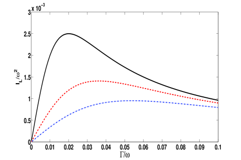
Figure 2: Current $I_{L}/\omega^{2}$ shown as a function of reservoir coupling strength $\Gamma/\omega$ for different atom-cavity coupling strengths $\chi/\omega=0$ (continuous), $0.03$ (dashed) and $0.05$ (dot-dashed). The system-reservoir parameters are $J/\omega=0.02,\bar{n}_{L}-\bar{n}_{R}=0.5$ and $\langle\sigma_{z}\rangle=1$.

III Negative thermal conductivity

According to the Fourier’s law given in Eqn. 1, current is proportional to temperature gradient. Using the fact that $\delta N\propto(\bar{n}_{L}-\bar{n}_{R})$ as given in Eqn. 15$c$, the expression for $I_{L}$ in Eqn. 17 can be written in the form

$$I_{L}=\tilde{\kappa}(\bar{n}_{L}-\bar{n}_{R}),$$ (25)

for comparing with the Fourier’s law. Here $\tilde{\kappa}$ is the effective thermal conductivity. It is to be noted that thermal conductivity can be tuned by suitably choosing the atomic state. Two important cases corresponding to the atom being in the excited state and the ground state are considered, i.e., $\langle\sigma_{z}\rangle=\pm 1$. The corresponding currents are

$$I_{L}=J^{2}\delta N\frac{\Omega}{(\chi^{2}-\Delta_{c}^{2}+\gamma^{2})^{2}+4\gamma^{2}\Delta_{c}^{2}}((\Delta_{c}\pm\chi)^{2}+\gamma^{2}).$$ (26)

where $\Omega=\omega_{L}\Gamma_{R}+\Gamma_{L}(\omega_{R}\pm\chi)$. We assume $\bar{n}_{L}>\bar{n}_{R}$, i.e., $\delta N>0$ for subsequent discussion. In this assumption, $I_{L}$ and $\Omega$ have the same sign. If the atom is in its ground state, sign of $\Omega$ is changeable by properly choosing the ratios $\Gamma_{R}/\Gamma_{L}$ and $(\chi-\omega_{R})/\omega_{L}$. Consequently, direction of current can also be changed. It is to be pointed out that $\omega_{R}-\chi$ is the resonance frequency of the right cavity modified by the atom. If the atom is in its excited state, i.e., $\langle\sigma_{z}\rangle=+1$, $I_{L}$ is always positive, meaning the thermal current flows from the high temperature reservoir to the low temperature reservoir (conventional flow) and reversal of current is not possible.

In order to exhibit the switching action by the atom, we choose $\chi>\omega_{R}$. If the system-reservoir parameters satisfy

$$\frac{\Gamma_{R}}{\Gamma_{L}}>\frac{(\chi-\omega_{R})}{\omega_{L}},$$ (27)

thermal current flows from the high temperature reservoir to the low temperature reservoir, independent of the atomic state.

If the ratios are equal, i.e.,

$$\frac{\Gamma_{R}}{\Gamma_{L}}=\frac{(\chi-\omega_{R})}{\omega_{L}},$$ (28)

and the atom is in the ground state, the thermal current through the system is zero even if the reservoirs are at different temperatures. The system completely blocks the heat flow like a thermal insulator. By switching the atom to its excited state, the system changes from a thermal-insulator to a thermal-conductor.

If the atom is in its ground state and the system-reservoir parameters are such that

$$\frac{\Gamma_{R}}{\Gamma_{L}}<\frac{(\chi-\omega_{R})}{\omega_{L}},$$ (29)

then $\Omega<0$ and the direction of thermal current reverses, i.e., current flows from low temperature reservoir to high temperature reservoir (unconventional flow). In such case, thermal conductivity of the system can be interpreted to be negative in which case heat flows from the low temperature to high temperature. Emergence of this negative current may be a result of coupling the system to Markovian baths Diehl et al. (2008). By switching the atom from its ground state to excited state, the unconventional flow of thermal current switches to the conventional flow. Thus, the atom acts as a thermal switch which brings about a controllable current flow through the cavities.

To summarize, we define

$$\alpha=\frac{\Gamma_{R}/\Gamma_{L}}{(\chi-\omega_{R})/\omega_{L}}.$$ (30)

The three conditions given in Eqns. (27-29) correspond to $\alpha$ becoming greater than, equal to or less than unity respectively. The signs of the respective currents established in the system are indicated in Table. 1.

Table 1: Conditions for positive and negative thermal currents.

	$~{}~{}\langle\sigma_{z}\rangle=+1~{}~{}$	$~{}~{}\langle\sigma_{z}\rangle=-1~{}~{}$
$~{}~{}\alpha>1~{}~{}$	$I_{L}>0$	$I_{L}>0$
$\alpha=1$	$I_{L}>0$	$I_{L}=0$
$\alpha<1$	$I_{L}>0$	$I_{L}<0$

Scaled current $I_{L}/I_{0}$ for the case of the atom in its ground state is shown as a function of $\chi/\omega_{L}$ in Fig. 3 for cavity-reservoir coupling ratios $\Gamma_{R}/\Gamma_{L}=0.1$ (continuous), $0.3$ (dashed) and $0.6$ (dot-dashed). Here $I_{0}$ is the amount of current flowing through the system when $\chi=0$. The inset figure shows the scaled current in the system when the atom is in excited state for the same values of $\Gamma_{R}/\Gamma_{L}$. Note that the current is always positive if the atom is in the excited state (inset figure). If the atom is in its ground state, current vanishes if the system and reservoir parameters satisfy Eqn. 28. Negative current occurs at different values of $\chi/\omega_{L}$ required to satisfy Eqn. 29.

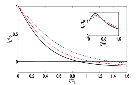
Figure 3: Normalized current $I_{L}/I_{0}$ shown as a function of $\chi/\omega_{L}$ for different cavity-reservoir coupling ratio $\Gamma_{R}/\Gamma_{L}=0.1$ (continuous), $0.3$ (dashed) and $0.6$ (dot-dashed). The system-reservoir parameters are $J/\omega_{L}=0.05,\bar{n}_{L}-\bar{n}_{R}=0.5,\omega_{R}/\omega_{L}=0.8$ and $\langle\sigma_{z}\rangle=-1$. The current in the system is shown in the inset for the same values of the parameters and $\langle\sigma_{z}\rangle=+1$.

Negative current arises because the contribution from the coherence part $I_{coh}$ is more than the current due to mean excitation number difference $I_{nd}$, which makes $I_{L}$ negative (refer Eqn. 13). Dimensionless quantities $I_{nd}/\omega_{L}^{2},I_{coh}/\omega_{L}^{2}$ and $I_{L}/\omega_{L}^{2}$ are shown in Fig. 4 as a function of the atom-field coupling strength $\chi/\omega_{L}$. It is to be noted that if the parameters are chosen to satisfy Eqn. 28, in which case $I_{nd}=I_{coh}$, the system completely blocks the current. Current reverses its direction from the low temperature reservoir to the high temperature reservoir when $I_{coh}>I_{nd}$. In this sense, the coherence in the system drives energy to flow to the high temperature reservoir.

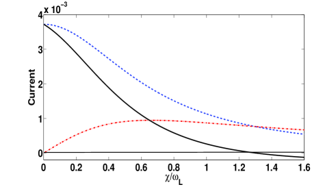
Figure 4: Dimensionless currents $I_{L}/\omega_{L}^{2}$(continuous), $I_{nd}/\omega_{L}^{2}$ (dashed) and $I_{coh}/\omega_{L}^{2}$ (dot-dashed) shown as function of $\chi/\omega_{L}$. Here $\Gamma_{R}/\Gamma_{L}=0.3$, $J/\omega_{L}=0.05,\bar{n}_{L}-\bar{n}_{R}=0.5,\omega_{R}/\omega_{L}=1$ and $\langle\sigma_{z}\rangle=-1$.

IV Thermal Rectification

Figure 5: Reverse configuration of system-reservoirs. reservoir temperatures and the system-reservoir coupling strengths are interchanged.

A system exhibits thermal rectification if thermal current depends on the direction of heat flow,

$$I(\Delta n)\neq-I(-\Delta n),$$ (31)

where $\Delta n=\bar{n}_{L}-\bar{n}_{R}$ is the difference in the average photon number of the left and right reservoirs. This means that by swapping the thermal reservoirs, current changes both sign and magnitude.

If the system is symmetric under the exchange of cavities, rectification is not possible. In the system under discussion, assymmetry is due to presence of the atom in one of the cavities. Thermal rectification is to be established by studying the transport of photon in the reverse configuration realized by interchanging the reservoirs and system-reservoir coupling strengths. The reverse configuration is shown in Fig. 5. The relevant Lindblad operators for the reverse configuration are

$$\mathcal{D}_{L}(\rho)= \frac{\Gamma_{R}(\bar{n}_{R}+1)}{2}(2a_{L}\rho a_{L}^{\dagger}-a_{L}^{\dagger}a_{L}\rho-\rho a_{L}^{\dagger}a_{L})$$

$$+\frac{\Gamma_{R}\bar{n}_{R}}{2}(2a_{L}^{\dagger}\rho a_{L}-a_{L}a_{L}^{\dagger}\rho-\rho a_{L}a_{L}^{\dagger}),$$

$$\mathcal{D}_{R}(\rho)= \frac{\Gamma_{L}(\bar{n}_{L}+1)}{2}(2a_{R}\rho a_{R}^{\dagger}-a_{R}^{\dagger}a_{R}\rho-\rho a_{R}^{\dagger}a_{R})$$

$$+\frac{\Gamma_{L}\bar{n}_{L}}{2}(2a_{R}^{\dagger}\rho a_{R}-a_{R}a_{R}^{\dagger}\rho-\rho a_{R}a_{R}^{\dagger}).$$

The atom is taken to be in its ground state. Steady state solutions for the expectation values of operators for the reverse configuration can be obtained by the transformations $\Gamma_{L}\longrightarrow\Gamma_{R}$, $\bar{n}_{L}\longrightarrow\bar{n}_{R}$ and vice-versa in Eqns. 15$a$-15$d$.

Current from the left reservoir $R_{L}$ to the right reservoir $R_{R}$ in the system shown in Fig. 1 is called forward current. The expression for the forward current is

$$I_{f}(\Delta n,\Gamma_{L},\Gamma_{R})=J^{2}\delta N\frac{(\omega_{L}\Gamma_{R}+\Gamma_{L}(\omega_{R}-\chi))}{(\chi^{2}-\Delta_{c}^{2}+\gamma^{2})^{2}+4\gamma^{2}\Delta_{c}^{2}}((\Delta_{c}-\chi)^{2}+\gamma^{2}).$$ (32)

On exchanging ($\bar{n}_{L},\Gamma_{L})$ and $(\bar{n}_{R},\Gamma_{R})$, reverse current from the right reservoir $R_{R}$ to the left reservoir $R_{L}$ in the configuration given in Fig. 5 is

$$I_{r}(-\Delta n,\Gamma_{R},\Gamma_{L})=-J^{2}\delta N\frac{(\omega_{L}\Gamma_{L}+\Gamma_{R}(\omega_{R}-\chi))}{(\chi^{2}-\Delta_{c}^{2}+\gamma^{2})^{2}+4\gamma^{2}\Delta_{c}^{2}}((\Delta_{c}-\chi)^{2}+\gamma^{2}).$$ (33)

The reverse current is taken as negative as the direction of flow is opposite to the forward current. The currents $I_{f}$ and $I_{r}$, normalized with their corresponding values for $\chi=0$ and $\Delta_{c}=0$, are shown as a function of the atom-field coupling strength $\chi$ in Fig. 6. For non-zero $\chi$, the magnitudes of the forward and reverse currents are different. Therefore, the system shows thermal rectification. Importantly, if the parameters satisfy the condition given in Eqn. 29, the forward current changes the sign. As a result, $I_{f}$ and $I_{r}$ flow in same direction.

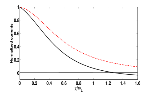
Figure 6: Normalized forward current $I_{f}$ (continuous line) and reverse current $I_{r}$ (dashed line) as a function of $\chi/\omega_{L}$ for $\Gamma_{R}/\Gamma_{L}=0.3$. Currents are normalized with their respective values at $\chi=0$. The system-reservoir parameters are $J/\omega_{L}=0.05,\bar{n}_{L}-\bar{n}_{R}=0.5,\omega_{R}/\omega_{L}=1$ and $\langle\sigma_{z}\rangle=-1$.

Thermal rectification is quantified by rectification coefficient $R$ defined as

$$R=-\frac{I_{f}}{I_{r}}.$$ (34)

If $R=1$, there is no rectification. For the system under consideration

$$R=\frac{\omega_{L}\Gamma_{R}+\Gamma_{L}(\omega_{R}-\chi)}{\omega_{L}\Gamma_{L}+\Gamma_{R}(\omega_{R}-\chi)}.$$ (35)

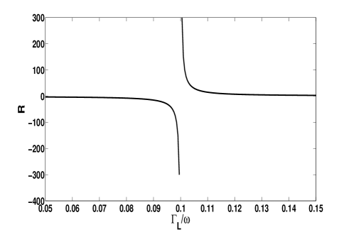
Figure 7: Rectification $R$ as a function of $\Gamma_{L}/\omega$ for $\Gamma_{R}/\omega=0.2$. Here $\chi/\omega=1.5$ and $\langle\sigma_{z}\rangle=-1$.

If $\Gamma_{L}=\Gamma_{R}$ or $\omega_{L}=|\omega_{R}-\chi|$, rectification coefficient $R$ becomes unity. Rectification coefficient $R$ is shown as a function of $\Gamma_{L}/\omega$ in Fig. 7 for the resonant case ($\Delta_{c}=0$). Rectification is positive, zero, or negative depending on the parameters. The system shows large rectification if

$$\frac{\Gamma_{L}}{\Gamma_{R}}=\frac{\chi-\omega_{R}}{\omega_{L}},$$ (36)

as seen in Fig. 7. This originates from the fact that the atom completely blocks the current in one direction (thermally insulating) and allows in the other direction (thermally conducting). Even though the system size is finite, rectification becomes infinity theoretically. If $\Gamma_{L}/\omega$ is increases from values less than that satisfying Eqn. 36 to higher values, $R$ jumps from negative value of large magnitude to large positive value. Thus $R$ is very sensitive to changes in the parameters in that region. Asymmetry can also be introduced with non-resonant cavities without an atom $(\chi=0)$ in any of the cavities. However, as seen from Eqn. 35, large rectification is not possible.

V Generalization to $N$-cavities

It would be interesting to study the steady state heat transfer in $N$ coupled cavities containing a two-level atom in one of the cavities. The Hamiltonian for the system is

$$\tilde{H}=\frac{\omega_{0}}{2}\sigma_{z}+\omega\sum_{j=1}^{N}a_{j}^{\dagger}a_{j} +J\sum_{j=1}^{N-1}(a_{j}^{\dagger}a_{j+1}+a_{j}a_{j+1}^{\dagger})$$

$$+\chi(\sigma_{+}\sigma_{-}+a^{\dagger}_{m}a_{m}\sigma_{z}).$$ (37)

The atom is embedded in the $m$th cavity and dispersively interacts with the cavity-field. The right most and the left most cavities in the array are coupled with two reservoirs $R_{L}$ and $R_{R}$ respectively. The density matrix $\tilde{\rho}$ of the system obeys

$$\frac{\partial\tilde{\rho}}{\partial t}=-i[\tilde{H},\tilde{\rho}]+\mathcal{D}_{L}(\tilde{\rho})+\mathcal{D}_{R}(\tilde{\rho}),$$ (38)

where

$$\mathcal{D}_{L}(\tilde{\rho})= \frac{\Gamma_{L}(\bar{n}_{L}+1)}{2}(2a_{1}\tilde{\rho}a_{1}^{\dagger}-a_{1}^{\dagger}a_{1}\tilde{\rho}-\tilde{\rho}a_{1}^{\dagger}a_{1})$$

$$+\frac{\Gamma_{L}\bar{n}_{L}}{2}(2a_{1}^{\dagger}\tilde{\rho}a_{1}-a_{1}a_{1}^{\dagger}\tilde{\rho}-\tilde{\rho}a_{1}a_{1}^{\dagger}),$$

$$\mathcal{D}_{R}(\tilde{\rho})= \frac{\Gamma_{R}(\bar{n}_{R}+1)}{2}(2a_{N}\tilde{\rho}a_{N}^{\dagger}-a_{N}^{\dagger}a_{N}\tilde{\rho}-\tilde{\rho}a_{N}^{\dagger}a_{N})$$

$$+\frac{\Gamma_{R}\bar{n}_{R}}{2}(2a_{N}^{\dagger}\tilde{\rho}a_{N}-a_{N}a_{N}^{\dagger}\tilde{\rho}-\tilde{\rho}a_{N}a_{N}^{\dagger}),$$

Here $\bar{n}_{L}$ and $\bar{n}_{R}$ are the mean number of photons in the reservoirs $R_{L}$ and $R_{R}$ respectively. Without loss of generality, we assume $\bar{n}_{L}>\bar{n}_{R}$.

Using Eqn. 38, the equation of motion is

$$\frac{d\langle G\rangle}{dt}=\frac{d}{dt}\text{Tr}(\tilde{\rho}G)=i[M_{1},\langle G\rangle]+\{M_{2},\langle G\rangle\}+M_{3},$$ (39)

where $\langle G\rangle=\langle A^{\dagger}A\rangle$ is the matrix whose elements are the expectation values of the operator elements of $A^{\dagger}A$. Here

$$A =\text{Row}(a_{1},a_{2},...a_{N},a_{1}\sigma_{z},...,a_{N}\sigma_{z}),$$

$$A^{\dagger} =\text{Column}(a_{1}^{\dagger},a_{2}^{\dagger},...a_{N}^{\dagger},a_{1}^{\dagger}\sigma_{z},...,a_{N}^{\dagger}\sigma_{z}).$$

Further $[M_{1},\langle G\rangle]=M_{1}\langle G\rangle-\langle G\rangle M_{1}$ and $\{M_{2},\langle G\rangle\}=M_{2}\langle G\rangle+\langle G\rangle M_{2}$. The transformation matrices are

$$M_{1}= I_{2\times 2}\otimes H_{c}+\sigma_{x}\otimes X,$$

$$M_{2}= I_{2\times 2}\otimes\text{Diag}\left(-\frac{1}{2}\Gamma_{L},0,...0,-\frac{1}{2}\Gamma_{R}\right)_{N\times N},$$

$$M_{3}= I_{2\times 2}\otimes\text{Diag}\left(\Gamma_{L}\bar{n}_{L},0,...0,\Gamma_{R}\bar{n}_{R}\right)_{N\times N}$$

$$~{}~{}~{}~{}~{}~{}+\sigma_{x}\otimes\text{Diag}(\Gamma_{L}\bar{n}_{L}\langle\sigma_{z}\rangle,0,...0,\Gamma_{R}\bar{n}_{R}\langle\sigma_{z}\rangle)_{N\times N},$$

where $I_{2\times 2}$ is the identity matrix of dimension $2$ and $\sigma_{x}$ is the Pauli matrix. The matrix

$$H_{c}=\left(\begin{matrix}\omega&J&0&\ldots&0\\ J&\omega&J&\ldots&0\\ \vdots&\vdots&\ddots&\vdots\\ 0&0&\ldots&\omega&J\\ 0&0&\ldots&J&\omega\end{matrix}\right)_{N\times N},$$

and the matrix elements of $(X)_{N\times N}$ are zero except $X_{m,m}=\chi$.

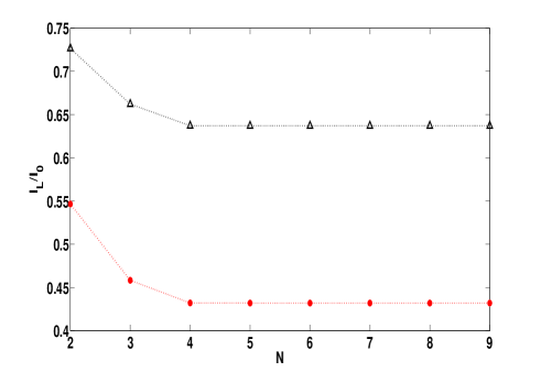
Figure 8: Ratio of currents $I_{L}/I_{0}$ as a function of $N$ for $\chi/\omega=0.15$ (circle) and $0.1$ (triangle). The atom is embedded in the last cavity ($m=N$). Here $J/\omega=0.05,\bar{n}_{L}-\bar{n}_{R}=0.5,\langle\sigma_{z}\rangle=-1,\Gamma_{L}/\omega=\Gamma_{R}/\omega=0.15$.

Using $\tilde{H}$ given in Eqn. V in the continuity equation (refer Eqn. 11), the current in the system is

$$I_{L}=\Gamma_{L}\left[(\bar{n}_{L}-\right. \langle a_{1}^{\dagger}a_{1}\rangle_{ss})(\omega+\chi\langle\sigma_{z}\rangle\delta_{m,1})$$

$$\left.-\frac{J}{2}(\langle a_{1}^{\dagger}a_{2}\rangle_{ss}+\langle a_{1}a_{2}^{\dagger}\rangle_{ss})\right].$$ (40)

Here $\delta_{m,1}$ is Kronecker delta. If there is no atom in the array, the coherence term $\langle a_{j}^{\dagger}a_{j+1}\rangle$ is purely imaginary Asadian et al. (2013). The contribution of the coherence term to the current vanishes as $I_{coh}=\frac{J}{2}(\langle a_{1}^{\dagger}a_{2}\rangle_{ss}+\langle a_{1}a_{2}^{\dagger}\rangle_{ss})=0$. Consequently, current in the cavity array is

$$I_{L}(\chi=0)=I_{0}=\frac{4\omega J^{2}\Gamma_{L}\Gamma_{R}}{(4J^{2}+\Gamma_{L}\Gamma_{R})(\Gamma_{L}+\Gamma_{R})}(\bar{n}_{L}-\bar{n}_{R}).$$ (41)

Note that the current $I_{0}$ is independent of the size of the array, in violation of Fourier’s law. This feature is similar to the system-size independent current in the case of ballistic transport Zürcher and Talkner (1990); Gaul and Büttner (2007); Asadian et al. (2013). This comparison indicates that the mean free path of the photons scales in proportion to the number of cavities $N$.

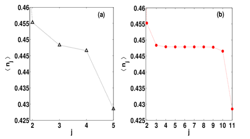
Figure 9: Steady state mean photon number in the intermediate cavities for arrays of length $(a)N=6$ and $(b)N=12$. The atom-field coupling strength is chosen to be $\chi/\omega=0.1$. Here $J/\omega=0.05,\bar{n}_{L}-\bar{n}_{R}=0.5,\langle\sigma_{z}\rangle=-1,\Gamma_{L}/\omega=\Gamma_{R}/\omega=0.15$.

Mean free path is different from the array size if an atom is embedded in one of the cavities. The atom is considered to be in the last cavity of the array, i.e., $m=N$, to keep the mean free path as close to the size of the array. This helps to understand the emergence of diffusive character if there is a single scatterer. The normalized current $I_{L}/I_{0}$ as a function of size of the array $N$ is shown in Fig. 8 for a fixed temperature difference $(\bar{n}_{L}-\bar{n}_{R})$. It is to be noted that by increasing the size of the array, the steady state current significantly decreases and asymptotically approaches a constant value. The current is size dependent for smaller array. Thus the atom is able to introduce diffusive character. It saturates with further increase in size and becomes nearly size independent, which is at odds with the Fourier’s law. Thus, the transport is of ballistic type. If many cavities in the array contain atoms, the heat transport may be expected to be diffusive. This is plausible as the effect of dephasing by all the atoms effectively reduces the mean free path for the photons Brune et al. (1996); Asadian et al. (2013).

The transition from diffusive to ballistic transport as size of the array increases, can be understood by calculating the mean photon numbers $\langle n_{j}\rangle=\langle a_{j}^{\dagger}a_{j}\rangle$ (known as local temperature Asadian et al. (2013)) of the respective cavities in the array. The steady state mean photon number $\langle n_{j}\rangle$ in the intermediate cavities for arrays containing $6$ and $12$ cavities are shown in Fig. 9$(a)$ and $(b)$ respectively. Gradient in the mean photon number is noticed in Fig. 9$(a)$. This implies that the transport is diffusive Rieder et al. (1967); Hu et al. (1998). For larger size array, for instance $N=12$, the gradient in mean photon number approaches zero and the current is independent of the system size. Essentially, the change in mean free path in the presence of a scatterer at the end of the array is insignificant for large array. Consequently, the photon transport is not diffusive.

VI Summary

Mesoscopic systems offer interesting possibilities when it comes to thermal properties. A system of two coupled cavities connected between thermal reservoirs provides a conduit for heat flow between the reservoirs. If a dispersively interacting atom is placed in one of the cavities, thereby providing an asymmetry in the system, many of the thermal transport properties can be tailored. The present system switches from a thermally insulating state to a conducting one, depending on whether the atom is in its ground state or excited state. If the atomic state changes from the excited state to the ground state, current through the system becomes zero or reversed depending on the system-reservoir coupling strengths and the cavity frequencies. The reversal of current implies that the effective thermal conductivity is negative.

The presence of the atom changes the magnitude of the current on exchange of the reservoirs along with the coupling strengths, which leads to thermal rectification. Large rectification is possible if the parameters are chosen to make the system thermally resistive either for the forward current or the reverse current.

If a cavity array contains a two-level atom in one of the cavities, the magnitude of current depends on the number of cavities. This size-dependence indicates that the thermal current through the array is analogous to the diffusive heat transport. If there is only a single atom in a large array, it is not possible to completely recover the diffusive transport. Single atom does not provide enough dephasing to recover the diffusive character.

Data accessibilities
This paper has no data.
Competing interest
We have no competing interest.
Authors’ contribution
Both the authors formulated and analyzed the problem. Both contributed to the interpretation of the results.
Funding statement
There is no funding.
Ethics statement
It does not apply.

References

- Northup and Blatt (2014) T. E. Northup and R. Blatt, Nature Photonics 8, 356 (2014).
- Meher et al. (2017) N. Meher, S. Sivakumar, and P. K. Panigrahi, Scientific Reports 7, 9251 (2017).
- Zhong (2016) Z.-R. Zhong, Scientific Reports 6, 8 (2016).
- Yang et al. (2013) C.-P. Yang, Q.-P. Su, and F. Nori, New Journal of Physics 15, 115003 (2013).
- Majumdar et al. (2012) A. Majumdar, A. Rundquist, M. Bajcsy, V. D. Dasika, S. R. Bank, and J. Vučković, Phys. Rev. B 86, 195312 (2012).
- Almeida et al. (2016) G. M. A. Almeida, F. Ciccarello, T. J. G. Apollaro, and A. M. C. Souza, Phys. Rev. A 93, 032310 (2016).
- Biella et al. (2015) A. Biella, L. Mazza, I. Carusotto, D. Rossini, and R. Fazio, Phys. Rev. A 91, 053815 (2015).
- Liu and Zhou (2015) Y. Liu and D. L. Zhou, New Journal of Physics 17, 013032 (2015).
- Liao et al. (2010) J.-Q. Liao, Z. R. Gong, L. Zhou, Y.-x. Liu, C. P. Sun, and F. Nori, Phys. Rev. A 81, 042304 (2010).
- Liew and Savona (2012) T. C. H. Liew and V. Savona, Phys. Rev. A 85, 050301 (2012).
- Imamoḡlu et al. (1997) A. Imamoḡlu, H. Schmidt, G. Woods, and M. Deutsch, Phys. Rev. Lett. 79, 1467 (1997).
- Felicetti et al. (2014) S. Felicetti, G. Romero, D. Rossini, R. Fazio, and E. Solano, Phys. Rev. A 89, 013853 (2014).
- Qin and Nori (2016) W. Qin and F. Nori, Phys. Rev. A 93, 032337 (2016).
- Zhou et al. (2008) L. Zhou, Z. R. Gong, Y.-x. Liu, C. P. Sun, and F. Nori, Phys. Rev. Lett. 101, 100501 (2008).
- Brune et al. (1996) M. Brune, E. Hagley, J. Dreyer, X. Maître, A. Maali, C. Wunderlich, J. M. Raimond, and S. Haroche, Phys. Rev. Lett. 77, 4887 (1996).
- Brune et al. (1992) M. Brune, S. Haroche, J. M. Raimond, L. Davidovich, and N. Zagury, Phys. Rev. A 45, 5193 (1992).
- Schmidt et al. (2010) S. Schmidt, D. Gerace, A. A. Houck, G. Blatter, and H. E. Türeci, Phys. Rev. B 82, 100507 (2010).
- Meher and Sivakumar (2016) N. Meher and S. Sivakumar, J. Opt. Soc. Am. B 33, 1233 (2016).
- Manzano and Kyoseva (2016) D. Manzano and E. Kyoseva, Scientific Reports 6, 31161 (2016).
- Xuereb et al. (2015) A. Xuereb, A. Imparato, and A. Dantan, New Journal of Physics 17, 055013 (2015).
- Garrido et al. (2001) P. L. Garrido, P. I. Hurtado, and B. Nadrowski, Phys. Rev. Lett. 86, 5486 (2001).
- Dhar (2008) A. Dhar, Advances in Physics 57, 457 (2008).
- Saito (2003) K. Saito, EPL (Europhysics Letters) 61, 34 (2003).
- Michel et al. (2005) M. Michel, G. Mahler, and J. Gemmer, Phys. Rev. Lett. 95, 180602 (2005).
- Dubi and Di Ventra (2009) Y. Dubi and M. Di Ventra, Phys. Rev. E 79, 042101 (2009).
- Saito et al. (1996) K. Saito, S. Takesue, and S. Miyashita, Phys. Rev. E 54, 2404 (1996).
- Landi et al. (2014) G. T. Landi, E. Novais, M. J. de Oliveira, and D. Karevski, Phys. Rev. E 90, 042142 (2014).
- Schachenmayer et al. (2015) J. Schachenmayer, C. Genes, E. Tignone, and G. Pupillo, Phys. Rev. Lett. 114, 196403 (2015).
- Werlang and Valente (2015) T. Werlang and D. Valente, Phys. Rev. E 91, 012143 (2015).
- Manzano et al. (2012) D. Manzano, M. Tiersch, A. Asadian, and H. J. Briegel, Phys. Rev. E 86, 061118 (2012).
- Thingna et al. (2012) J. Thingna, J. L. García-Palacios, and J.-S. Wang, Phys. Rev. B 85, 195452 (2012).
- He et al. (2016) D. He, J. Thingna, J.-S. Wang, and B. Li, Phys. Rev. B 94, 155411 (2016).
- Asadian et al. (2013) A. Asadian, D. Manzano, M. Tiersch, and H. J. Briegel, Phys. Rev. E 87, 012109 (2013).
- Purkayastha et al. (2016a) A. Purkayastha, A. Dhar, and M. Kulkarni, Phys. Rev. A 94, 052134 (2016a).
- Li et al. (2004) B. Li, L. Wang, and G. Casati, Phys. Rev. Lett. 93, 184301 (2004).
- Li et al. (2006) B. Li, L. Wang, and G. Casati, Applied Physics Letters 88, 143501 (2006).
- Li et al. (2008) N. Li, P. Hänggi, and B. Li, EPL (Europhysics Letters) 84, 40009 (2008).
- Wang and Li (2007) L. Wang and B. Li, Phys. Rev. Lett. 99, 177208 (2007).
- Wang and Li (2008) L. Wang and B. Li, Phys. Rev. Lett. 101, 267203 (2008).
- Rieder et al. (1967) Z. Rieder, J. L. Lebowitz, and E. Lieb, Journal of Mathematical Physics 8, 1073 (1967).
- Zotos et al. (1997) X. Zotos, F. Naef, and P. Prelovsek, Phys. Rev. B 55, 11029 (1997).
- Hu et al. (1998) B. Hu, B. Li, and H. Zhao, Phys. Rev. E 57, 2992 (1998).
- Debnath et al. (2017) K. Debnath, E. Mascarenhas, and V. Savona, New Journal of Physics 19, 115006 (2017).
- Shah and Gajjar (2013) T. N. Shah and P. Gajjar, Communications in Theoretical Physics 59, 361 (2013).
- Starr (1936) C. Starr, Physics 7, 15 (1936).
- Chang et al. (2006) C. W. Chang, D. Okawa, A. Majumdar, and A. Zettl, Science 314, 1121 (2006).
- Zhang et al. (2009) L. Zhang, Y. Yan, C.-Q. Wu, J.-S. Wang, and B. Li, Phys. Rev. B 80, 172301 (2009).
- Yan et al. (2009) Y. Yan, C.-Q. Wu, and B. Li, Phys. Rev. B 79, 014207 (2009).
- Werlang et al. (2014) T. Werlang, M. A. Marchiori, M. F. Cornelio, and D. Valente, Phys. Rev. E 89, 062109 (2014).
- Terraneo et al. (2002) M. Terraneo, M. Peyrard, and G. Casati, Phys. Rev. Lett. 88, 094302 (2002).
- Segal and Nitzan (2005) D. Segal and A. Nitzan, Phys. Rev. Lett. 94, 034301 (2005).
- Lindblad (1976) G. Lindblad, Commun.Math. Phys. 48, 195452 (1976).
- Agarwal (2012) G. S. Agarwal, Quantum Optics (Cambridge University Press, 2012).
- Gerry (1996) C. C. Gerry, Phys. Rev. A 53, 2857 (1996).
- Holland et al. (1991) M. J. Holland, D. F. Walls, and P. Zoller, Phys. Rev. Lett. 67, 1716 (1991).
- Carmichael (1999) H. J. Carmichael, Statistical Methods in Quantum Optics 1: Master Equations and Fokker-Planck Equations (Springer, 1999).
- Gardiner and Zoller (2004) C. Gardiner and P. Zoller, Quantum Noise: A Handbook of Markovian and Non-Markovian Quantum Stochastic Methods with Applications to Quantum Optics (Springer, 2004).
- Diehl et al. (2008) S. Diehl, A. Micheli, A. Kantian, B. Kraus, H. P. Bucher, and P. Zoller, Nature Physics 4, 878 (2008).
- Biehs and Agarwal (2013) S.-A. Biehs and G. S. Agarwal, J. Opt. Soc. Am. B 30, 700 (2013).
- Rivas et al. (2010) A. Rivas, A. D. K. Plato, S. F. Huelga, and M. B. Plenio, New Journal of Physics 12, 113032 (2010).
- Purkayastha et al. (2016b) A. Purkayastha, A. Dhar, and M. Kulkarni, Phys. Rev. A 93, 062114 (2016b).
- Santos and Landi (2016) J. P. Santos and G. T. Landi, Phys. Rev. E 94, 062143 (2016).
- Zürcher and Talkner (1990) U. Zürcher and P. Talkner, Phys. Rev. A 42, 3278 (1990).
- Gaul and Büttner (2007) C. Gaul and H. Büttner, Phys. Rev. E 76, 011111 (2007).