Revival of the magnetar PSR J1622$-$4950: observations with MeerKAT, Parkes, XMM-Newton, Swift, Chandra, and NuSTAR 

Abstract

New radio (MeerKAT and Parkes) and X-ray (XMM-Newton, Swift, Chandra, and NuSTAR) observations of PSR J1622$-$4950 indicate that the magnetar, in a quiescent state since at least early 2015, reactivated between 2017 March 19 and April 5. The radio flux density, while variable, is approximately $100\times$ larger than during its dormant state. The X-ray flux one month after reactivation was at least $800\times$ larger than during quiescence, and has been decaying exponentially on a $111\pm 19$ day timescale. This high-flux state, together with a radio-derived rotational ephemeris, enabled for the first time the detection of X-ray pulsations for this magnetar. At 5%, the 0.3–6 keV pulsed fraction is comparable to the smallest observed for magnetars. The overall pulsar geometry inferred from polarized radio emission appears to be broadly consistent with that determined 6–8 years earlier. However, rotating vector model fits suggest that we are now seeing radio emission from a different location in the magnetosphere than previously. This indicates a novel way in which radio emission from magnetars can differ from that of ordinary pulsars. The torque on the neutron star is varying rapidly and unsteadily, as is common for magnetars following outburst, having changed by a factor of 7 within six months of reactivation.

=208

1 Introduction

Magnetars are the most magnetic objects known in the universe: a class of neutron stars with high-energy emission powered by the decay of ultra-strong magnetic fields, rather than through rotation (Thompson & Duncan, 1995). This is particularly manifest during large X-ray outbursts, when their luminosity exceeds that available from rotational spin down. The remarkable magnetar phenomenon provides a unique window into the behavior of matter at extreme energy densities. Although all confirmed magnetars spin slowly ($\approx 1$–10 s), it has been suggested that soon after birth, while spinning at millisecond periods, they could be responsible for some gamma ray bursts (e.g., Beniamini et al., 2017) or possibly fast radio bursts (e.g., Metzger et al., 2017).

Observations of both magnetars and rotation-powered pulsars are also uncovering links between the two populations. Camilo et al. (2006) discovered that magnetars can emit radio pulsations. Magnetar radio properties are often distinct from those of ordinary rotation-powered pulsars, e.g., in having flat radio spectra (e.g., Camilo et al., 2007c). On the other hand, while radio magnetars have highly variable pulse profiles, rotating vector model (RVM; Radhakrishnan & Cooke, 1969) fits to polarimetric observations often yield unexpectedly good results that suggest a magnetic field geometry at the location of emission not unlike that of ordinary pulsars (e.g., Camilo et al. 2008, but see also Kramer et al. 2007). Conversely, distinct magnetar-like outbursts, including short X-ray bursts and long-duration X-ray flux enhancements, have now been observed from two pulsars formerly classified as entirely rotation powered (Gavriil et al., 2008; Archibald et al., 2016).

Thus, more neutron stars that occasionally display magnetar behavior surely lurk amidst the $\approx 2500$ known “ordinary” pulsars. All the while, the careful study of the rotational and radiative behavior of the two dozen confirmed magnetars (Olausen & Kaspi, 2014), coupled with remarkable theoretical progress, continues to advance our understanding of these exceptional objects (for a recent review, see Kaspi & Beloborodov, 2017).

Only four magnetars are known to emit radio pulsations. The first to be identified, XTE J1810$-$197, remained an active radio source for approximately five years following the X-ray outburst that resulted in its discovery, and has been radio-dormant since, for nine years, while X-ray activity continues at a relatively low level (Camilo et al., 2016). Two others, 1E 1547.0$-$5408 and SGR 1745$-$2900, have remained very active radio and high-energy sources (e.g., Lynch et al., 2015; Coti Zelati et al., 2017; Mahrous, 2017, and references therein).

PSR J1622$-$4950, with rotation period $P=4.3$ s, remains the only magnetar discovered at radio wavelengths without prior knowledge of an X-ray counterpart (Levin et al., 2010). At the time of discovery, its X-ray flux was decaying exponentially from a presumed outburst in 2007, and no X-ray pulsations could be detected (Anderson et al., 2012). Detectable radio emission ceased in 2014 and, despite frequent monitoring, the pulsar remained undetectable through late 2016 (Scholz et al., 2017).

Here we report on new multi-wavelength observations of PSR J1622$-$4950, showing that the magnetar is once again in a highly active state. Observations with the CSIRO Parkes telescope first detected resumed radio emission on 2017 April 5. Subsequent observations with the new Square Kilometre Array South Africa (SKA SA) MeerKAT radio telescope have been tracking the unsteady spin-down torque, and, as we describe here, have enabled the first detection of X-ray pulsations for this neutron star through the folding of X-ray photons collected with Chandra and NuSTAR. Further X-ray observations with XMM-Newton and Swift provide a fuller view of the spectral evolution of the star following this most recent outburst.

2 Observations

2.1 Parkes

2.1.1 Monitoring

Following the last observation reported in Scholz et al. (2017), on 2016 September 16, we continued monitoring PSR J1622$-$4950 at the Parkes 64 m radio telescope. As before, the observations were performed with the PDFB4 digital filterbank in search mode, typically at a central frequency of 3.1 GHz (recording a bandwidth of 1 GHz), for $\approx 15$ minutes per session.

On 2017 April 26 we noticed during real-time monitoring of the observations that single pulses were being detected from the pulsar. Parkes underwent a planned month-long shutdown in May, and we started monitoring PSR J1622$-$4950 with MeerKAT in late April (Section 2.2.4).

2.1.2 Polarimetry

In order to compare the geometry of PSR J1622$-$4950 following its reactivation in 2017 with that before its disappearance by early 2015, we have made two calibrated polarimetric observations at the Parkes radio telescope, using PDFB4 in fold mode. These 40 minute observations were performed at 1.4 GHz (with 256 MHz bandwidth, on 2017 August 5) and 3.1 GHz (recording 1024 MHz of bandwidth, on August 16), using the center beam of the 20 cm multibeam receiver and the 10 cm band of the 1050cm receiver, respectively.

2.2 MeerKAT

MeerKAT, a precursor to the Square Kilometer Array (SKA), is a radio interferometer being built by SKA South Africa in the Karoo region of the Northern Cape province, at approximate coordinates $21^{\circ}26^{\prime}$ east, $30^{\circ}42^{\prime}$ south. The full array, scheduled to start science operations in 2018, will consist of 64 13.5 m diameter antennas located on baselines of up to 8 km. The observations reported in this paper were obtained during the commissioning phase and used a subset of the array and some interim subsystems. As MeerKAT is a new instrument not yet described in the literature, we provide here an overview of the system relevant to our results.

2.2.1 Receptors

The MeerKAT dishes are of a highly efficient unshaped “feed down” offset Gregorian design. This allows the positioning of four receiver systems on an indexing turret near the subreflector without compromising the clean optical path. A receptor consists of the primary reflector and subreflector, the feed horns, cryogenically cooled receivers and digitizers mounted on the feed indexer, as well as associated support structures and drive systems, all mounted on a pedestal. The observations reported here were performed at L band. Averaged across this 900–1670 MHz band, the measured system equivalent flux density (SEFD) of one receptor on cold sky is $\approx 460$ Jy. UHF (580–1015 MHz) and S-band (1.75–3.5 GHz) receiver systems are also being built (the latter by MPIfR).

The RF signal from the L-band receiver is transferred via coaxial cables to the shielded digitizer package $\sim 1$ m away. The digitizer samples the signal directly in the second Nyquist zone without heterodyne conversion. After RF conditioning and analog-to-digital conversion, the 10-bit voltage stream from each of two (horizontal and vertical) polarizations is framed into $4\times 10$ Gbps Ethernet streams. These are concatenated onto a single 40 Gbps stream for transmission via buried optical fiber cables to the central Karoo Array Processor Building (KAPB) located $<12$ km away. The one-pulse-per-second signal that allows precise time stamping of voltage sample data and the sample clock frequencies for the analog-to-digital converters (1712 MHz for L band) originate in the Time and Frequency Reference (TFR) subsystem located in the KAPB. Ultimately, two hydrogen maser clocks and time-transfer GPS receivers will allow time stamping to be traceable to within 5 ns of UTC. The observations presented here made use of an interim TFR system with GPS-disciplined rubidium clocks, which provides time stamps accurate to within 1 $\mu$s of UTC.

2.2.2 Correlator/Beamformer

The MeerKAT correlator/beamformer (CBF) implements an FX/B-style real-time signal processor in the KAPB. The antenna voltage streams are coarsely aligned as necessary to compensate for geometric and instrumental delays, split into frequency channels, and then phase aligned per frequency channel, prior to cross-correlation (X) and/or beamforming (B). This is done in the “F-engine” processing nodes, where a polyphase filterbank is used to achieve the required channelization with sufficient channel-to-channel isolation.

The CBF subsystem is based on the CASPER technology, which uses commodity network devices (in the case of MeerKAT, 40 Gbps Mellanox SX1710 36-port Ethernet switches arranged in a two-layer CLOS network yielding 384 ports) to handle digital data transfer and re-ordering between processing nodes. The switches allow a multicast of data to enable parallel processing. The processing nodes for the full MeerKAT array will consist of so-called SKARAB boards populated with Virtex 7 VX690T field-programmable gate arrays (FPGAs). The interim CBF, used for the observations presented here, uses the ROACH2 architecture populated with Virtex 6 SX475T FPGAs, and can handle a maximum of 32 inputs, such as two polarizations for each of 16 antennas.

For pulsar and fast transient applications, a tied-array beam is formed in the B engines, which perform coherent summation on previously delayed, channelized, and re-ordered voltage data. The F and B engines handle both polarizations, but polarization calibration still has to be implemented for tied-array mode, and the observations presented here are based on uncalibrated total-intensity time series.

2.2.3 Pulsar timing backend

For all observations presented here, data from a dual polarization tied-array beam split into 4096 frequency channels spanning 856 MHz of band centered at 1284 MHz were sent to the pulsar timing backend. This instrument is being developed by the Swinburne University of Technology pulsar group. The hardware consists of two eight-core servers, each equipped with four NVIDIA Titan X (Maxwell) GPUs, 128 GB of memory, a large storage disk, and dual-port 40 Gbps Ethernet interfaces, through which the beamformed data are received. This allows the simultaneous processing of up to four tied-array beams, although at present only one is provided by the B engines.

The beamformed voltage data stream is handled by a dedicated real-time pipeline. First, the UDP packets are received and allocated to a PSRDADA ring buffer. Next, the data are asynchronously transferred to the GPUs, dedispersed, detected, and folded into 1024 phase bins by DSPSR (van Straten & Bailes, 2011) using a TEMPO2 (Hobbs et al., 2006) phase predictor derived from the pulsar’s ephemeris. Every 10 s, a folded sub-integration is unloaded from the GPUs to local storage in PSRFITS format (Hotan et al., 2004) for subsequent offline analysis. Data acquisition and processing, as well as control and monitoring of the backend, are handled by SPIP, a C++, PHP and python software framework that combines the individual software tools mentioned above into a complete pulsar timing instrument. In the observations presented here, the data were dedispersed incoherently, although provision exists for coherent dedispersion.

2.2.4 MeerKAT observations

Table 1: X-Ray Observations of PSR J1622$-$4950 Since Its 2017 Outburst

Telescope	Energy	ObsID	Date	Start Time	Exposure Time
	(keV)		(YYYY-Month-DD)	(MJD)	(ks)
Swift	0.2–10	00010071001	2017 Apr 27	57870.7	2.5
Swift	0.2–10	00010071002	2017 May 01	57874.7	5.0
Swift	0.2–10	00010071003	2017 May 05	57878.7	1.7
NuSTAR	3–79	80202051002	2017 May 07	57880.9	52.6
Chandra	0.3–10	19214	2017 May 08	57881.8	10.1
Chandra	0.3–10	19215	2017 May 23	57896.2	15.0
NuSTAR	3–79	80202051004	2017 May 25	57898.5	69.5
NuSTAR	3–79	80202051006	2017 Aug 30	57995.1	124.9
Chandra	0.3–10	19216	2017 Sep 03	57999.4	25.0

We commenced observations of PSR J1622$-$4950 with MeerKAT on 2017 April 27. In a typical session, following successful array configuration we observed the calibrator PKS 1934$-$638, in order to derive and apply the phase-delay corrections.

Since the phase stability of the array is still being investigated, on each day we typically did three 20 minute magnetar observations interspersed with observations of PKS 1934$-$638. From April 27 to October 3 (a span of 159 days) we obtained a total of 231 such observations on 74 separate days. On average these used 14.4 antennas (on a variety of baselines dependent on availability). This corresponds to a cold-sky tied-array $\mbox{SEFD}\approx 32$ Jy, which is comparable to the equivalent Parkes telescope SEFD at L band (e.g., Manchester et al., 2001).

We preceded the magnetar observations on each day by a five minute track on PSR J1644$-$4559 ($P=0.45$ s, dispersion measure $\mbox{DM}=478$ cm^-3 pc), a bright pulsar with a known timing solution, to serve as a timing calibrator.

2.3 XMM-Newton 

The XMM-Newton X-ray telescope (Jansen et al., 2001) observed PSR J1622$-$4950 on 2017 March 19 for a total of 125 ks. During the observation the EPIC (European Photon Imaging Camera) pn camera (Strüder et al., 2001) was operated in Full Frame mode, while the EPIC MOS cameras (Turner et al., 2001) were operated in Small Window mode. The EPIC detectors are sensitive to energies of 0.15–15 keV.

Standard XMM-Newton data reduction threads were used to process the data using the Science Analysis Software (SAS) version 16. After removing the effects of soft proton flares, the usable live time was 102 ks. We used a circular source extraction region with radius 18″ centered on the pulsar, and the background was estimated from a circular source-free region of radius 72″.

2.4 Swift 

Three observations of PSR J1622$-$4950 were made with the Swift X-ray Telescope (XRT; Burrows et al., 2005) between 2017 April 27 and May 5. The first observation was made in Photon Counting (PC) mode, while the others were made in Windowed Timing (WT) mode. PC mode gives two-dimensional imaging capabilities at 2.5 s resolution, while WT provides only one spatial dimension but at a higher time resolution of 1.7 ms. More observational details are given in Table 1.

The observations were analyzed by running the standard XRT data reduction pipeline xrtpipeline on the pulsar position (see Table 2). For the PC mode observation, the source region was a circle of radius 20 pixels (0$\farcm$78) centered on the pulsar, while the background region was an annulus with an inner radius of 40 pixels and an outer radius of 60 pixels centered on the pulsar. For WT mode observations, the source regions were 40-pixel strips centered on the pulsar, and the background regions were 40-pixel strips placed away from the pulsar.

2.5 Chandra 

The Chandra X-ray Observatory (Weisskopf et al., 2000) observed PSR J1622$-$4950 on 2017 May 8 and 23, and September 3, using the ACIS-S (Garmire et al., 2003) spectrometer (see Table 1). All observations were made in Continuous Clocking (CC) mode. CC mode foregoes two-dimensional imaging to provide 2.85 ms time resolution.

The Chandra Interactive Analysis of Observations software (CIAO; Fruscione et al., 2006) was used to reduce the data. The data, downloaded from the Chandra Data Archive (CHASER), were first reprocessed using the script chandra_repro, and then the appropriate science thread was followed. Spectra were extracted using an 8-pixel (8″) strip centered on the pulsar. The background region was a 32-pixel strip placed away from the pulsar. Photon arrival times were corrected to the solar system barycenter using the pulsar position.

2.6 NuSTAR 

PSR J1622$-$4950 was observed with NuSTAR (Nuclear Spectroscopic Telescope Array; Harrison et al., 2013) on 2017 May 7 and 25, and August 30 (see Table 1). These observations were coordinated with Chandra (see Section 2.5), in order to probe the pulsar over a broad energy range.

The data were processed using the standard HEASOFT tools nupipeline and nuproducts, following the NuSTAR Quickstart Guide. Spectra from both Focal Plane Modules (FPMA and FPMB) were fit jointly during the analysis. Source regions were chosen to be circles with radii of 20 pixels (8′) centered on the pulsar. Background regions were circles of the same radius, but placed away from the pulsar. Event arrival times were corrected to the solar system barycenter using the pulsar position.

3 Analysis and Results

3.1 Radio Reactivation

After recognizing on 2017 April 26 that PSR J1622$-$4950 was emitting radio waves, we inspected the previously acquired Parkes monitoring data (Section 2.1.1). Data collected on April 5 showed that the pulsar had turned on (see Figure 1a). Our only other prior unpublished Parkes monitoring observations, from 2016 November 17 and 2017 January 14, show no evidence of pulsations, with a 5 $\sigma$ flux density limit of $\approx 0.3$ mJy at 3 GHz (see Scholz et al., 2017).

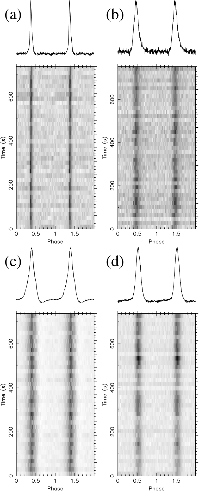
Figure 1: Radio pulse profiles of PSR J1622$-$4950. (a) Parkes at 3.1 GHz (bandwidth $\mbox{BW}=1$ GHz) on 2017 April 5. (b) MeerKAT at 1.3 GHz (RFI-free $\mbox{BW}\approx 500$ MHz) on April 27. (c) Parkes at 3.1 GHz ($\mbox{BW}=1$ GHz) on July 4. (d) Parkes at 1.4 GHz ($\mbox{BW}=256$ MHz) on June 7. All profiles are displayed (in arbitrary units) as a function of time and summed at the top, repeated twice. The baselines of the profiles in panels (c) and (d) are affected by instrumental artifacts.

3.2 Polarimetry

The fold-mode data on PSR J1622$-$4950 collected with PDFB4 in 2017 (Section 2.1.2) were analyzed with PSRCHIVE (Hotan et al., 2004) as in, e.g., Camilo et al. (2007b). The individually determined rotation measures (RMs) are essentially consistent with the value published in Levin et al. (2010), and the calibrated pulse profiles are shown in Figure 2. The period-averaged flux densities for these two observations (which are the only flux-calibrated radio observations presented in this paper) are $S_{1.4}=63\pm 6$ mJy and $S_{3}=32\pm 3$ mJy, respectively.

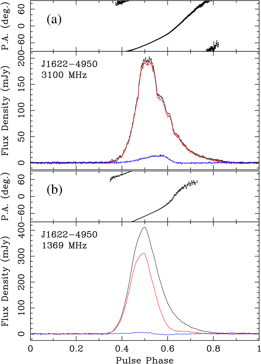
Figure 2: Calibrated full-Stokes profiles of PSR J1622$-$4950 based on Parkes observations. The red and blue lines represent the amount of linear and circular polarization, respectively, and the black traces show total intensity. The position angles (PAs) of linear polarization have been corrected for rotation measure $\mbox{RM}=-1495\pm 5$ rad m^-2 and are plotted de-rotated to infinite frequency. The profiles, from 2017 August 5 (panel (b)) and August 16 (panel (a)), are aligned by eye.

3.3 Radio Timing

The MeerKAT observations (Section 2.2.4) were used to obtain timing solutions for two purposes: to fold the Chandra and NuSTAR X-ray photons, and to probe the short-term variability of the spin-down torque on the neutron star.

All MeerKAT observations were processed in a homogeneous way using PSRCHIVE. The first few days of Parkes and MeerKAT observations (see Figure 1b) were used to improve the rotational ephemeris thereafter used to fold all MeerKAT observations.

Radio frequency interference (RFI) was excised in a multi-step process: first, 10% of the recorded band was removed due to bandpass roll-off, yielding the nominal 900–1670 MHz MeerKAT L band; next, a mask with known persistent RFI signals (e.g., GSM, GPS) was applied to the data; finally, PSRCHIVE tools and clean.py, an RFI-excision script provided by the CoastGuard data analysis pipeline (Lazarus et al., 2016), were used to remove remaining RFI. More than 400 MHz of clean band was typically retained after this flagging.

We summed all frequency channels, integrations, and polarizations for each observation to obtain total-intensity profiles. We then obtained times-of-arrival (TOAs) for each observation (i.e., two or three per day) by cross-correlating individual profiles with a standard template based on a very high signal-to-noise ratio observation.

The same procedure was applied to MeerKAT observations of PSR J1644$-$4559. Using the TEMPO software we confirmed that the timing solution derived for PSR J1644$-$4559 was consistent with published parameters (see Manchester et al., 2005).

Like many magnetars, PSR J1622$-$4950 displays unsteady rotation (e.g., Dib & Kaspi, 2014). Nevertheless, we were able to obtain a simple phase-connected timing solution for the three week period spanning the first two sets of paired Chandra and NuSTAR observations (Table 1), fitting the TOAs with TEMPO to a model containing only pulse phase, rotation frequency ($\nu$), and frequency derivative ($\dot{\nu}$). This solution is presented in Table 2.

Table 2: PSR J1622$-$4950 Ephemeris Used to Fold the X-Ray Data

Parameter	Value
R.A. (J2000)	$16^{\mathrm{h}}22^{\mathrm{m}}44\fs 89$
Decl. (J2000)	$-49\arcdeg 50\arcmin 52\farcs 7$
Spin frequency, $\nu\ (\text{s}^{-1})$	$0.231090389(2)$
Frequency derivative, $\dot{\nu}\ (\text{s}^{-2})$	$-7.94(2)\times 10^{-13}$
Epoch of frequency (MJD TDB)	57881
Data span (MJD)	57880–57903
Number of TOAs	59
rms residual (phase)	0.005
Derived Parameters
Spin-down luminosity, $\dot{E}$ (erg s-1)	$7.2\times 10^{33}$
Surface dipolar magnetic field, $B$ (G)	$2.6\times 10^{14}$
Characteristic age, $\tau_{c}$ (kyr)	4.6

Note. — Numbers in parentheses are TEMPO $1\,\sigma$ uncertainties.

Over the 5-month span of all the radio timing observations presented here, the $\dot{\nu}$ for PSR J1622$-$4950 has changed by a factor of 7, and $\ddot{\nu}$ has changed sign. In order to probe the evolution of the spin-down torque ($\propto\dot{\nu}$), we fit short-term overlapping timing models where a fit for $\nu$ and $\dot{\nu}$ proves adequate, i.e., with featureless timing residuals. Each of these short-term timing solutions spanned approximately one week. Figure 3 shows the run of $\dot{\nu}$ from these solutions spanning five months.

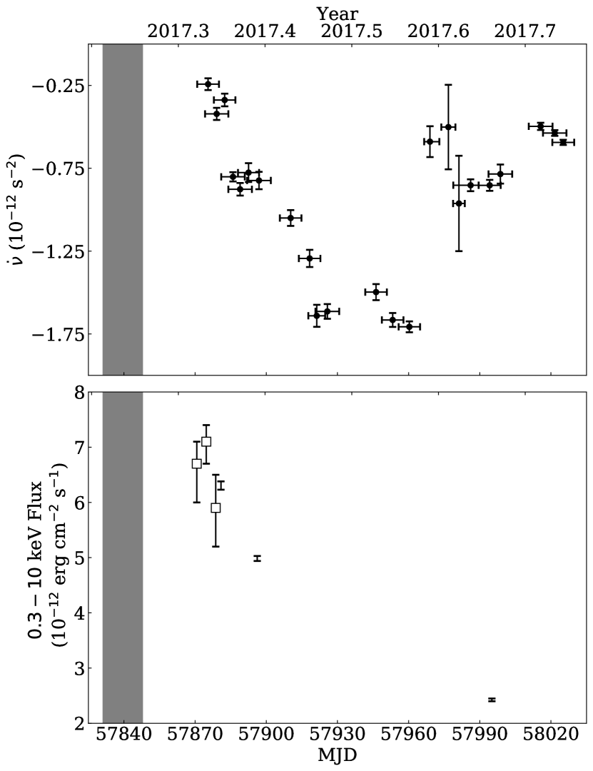
Figure 3: Time evolution of properties of PSR J1622$-$4950. Top panel: frequency derivative measured from short-term timing solutions (spanning horizontal error bars) obtained from MeerKAT data (see Section 3.3). Bottom panel: 0.3–10 keV absorbed X-ray flux as measured from the best-fit blackbody model (see Table 3). Swift observations are shown as open squares and combined Chandra and NuSTAR observations are represented simply by their error bars. The X-ray flux appears to be decaying exponentially with a time constant of $111\pm 19$ days (see Section 4.4). All error bars represent $1\,\sigma$ confidence levels. The gray band in both panels represents the timespan during which the X-ray outburst and radio revival most likely occurred (see Section 4).

3.4 Pre-outburst XMM-Newton Limit

In the 2017 March 19 XMM-Newton observation, performed before the April 5 observation that detected resumed radio activity from PSR J1622$-$4950, we detect no X-ray counts in excess of the background rate. Using the Bayesian method of Kraft et al. (1991), we place an upper limit of 0.002 s^-1 on the background-subtracted EPIC-pn 0.3–10 keV count-rate at a $5\,\sigma$ confidence level. (We use only the pn data to place an upper limit as the MOS detectors are much less sensitive.) For this limit, WebPIMMS gives a 0.3–10 keV absorbed flux limit of $9\times 10^{-15}$ erg cm^-2 s^-1, assuming an absorbed blackbody (BB) spectrum with $kT=0.4$ keV (typical of a quiescent magnetar; Olausen et al., 2013) and $N_{\text{H}}=6.4\times 10^{22}\,\text{cm}^{-2}$ (see Section 3.6). The corresponding $5\,\sigma$ unabsorbed flux limit is $8\times 10^{-14}$ erg cm^-2 s^-1.

3.5 X-Ray Pulsations

We have used the radio-derived rotational ephemeris presented in Table 2 to fold barycentered photons from the first two sets of paired Chandra and NuSTAR observations, and we clearly detect pulsations (Figure 4). To maximize the significance of the detected pulsations, we optimize the energy range that maximizes the $H$ statistic of the pulse (dsr89). For Chandra we find the optimal range to be 0.3–6.0 keV, with a false alarm probability, given the maximum value of the $H$ statistic, of $P_{\rm fa}=2\times 10^{-5}$ (equivalent to a $4.3\,\sigma$ detection). For NuSTAR we find the optimal range to be 2.0–8.0 keV ($P_{\rm fa}=1\times 10^{-7}$; $5.3\,\sigma$). We also present a combined Chandra and NuSTAR 0.3–8 keV profile which shows a strong pulse ($P_{\rm fa}=5\times 10^{-12}$; $6.9\,\sigma$). Note, however, that NuSTAR is not sensitive to X-ray photons below $\sim 2$ keV. This is the first detection of X-ray pulses from PSR J1622$-$4950. The pulsed fraction (PF) of the 0.3–6 keV Chandra profile is $\mbox{PF}=5\%\pm 1\%$ (using the RMS method described in An et al. 2015 Appendix A, where PF errors are reported at the $1\,\sigma$ level). For the 2–8 keV NuSTAR pulsations, $\mbox{PF}=4.1\%\pm 0.7\%$. This is far below the $3\,\sigma$ upper limit of $\mbox{PF}<70\%$ at 0.3–4 keV determined by Anderson et al. (2012).

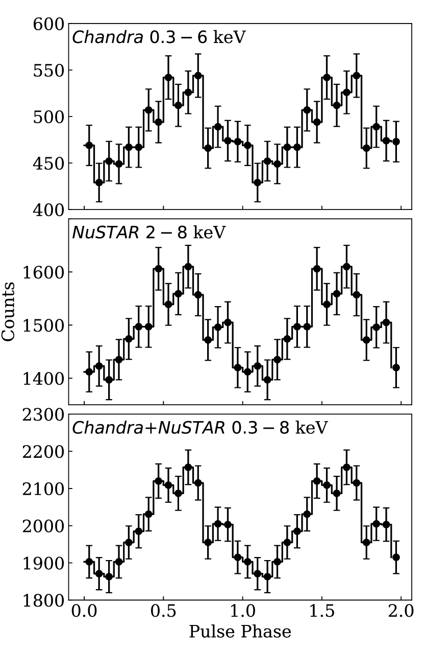
Figure 4: X-ray pulse profiles of PSR J1622$-$4950. Data from the first two sets of paired Chandra and NuSTAR observations were folded with the ephemeris from Table 2 (see Section 3.5). The top two panels show individual instrument profiles in the noted energy ranges. The bottom panel shows the overall combined profile.

Table 3: Spectral Fits for X-Ray Detections of PSR J1622$-$4950 in 2017

Telescope	ObsID	Start Time	0.3–10 keV Absorbed Flux	$kT$
		(MJD)	($10^{-12}$ erg cm-2 s-1)	(keV)
Swift	00010071001	57870.7	$6.7\begin{subarray}{c}+0.4\\ -0.7\end{subarray}$	$0.80\pm 0.04$
Swift	00010071002	57874.7	$7.1\begin{subarray}{c}+0.3\\ -0.4\end{subarray}$	$0.77\pm 0.03$
Swift	00010071003	57878.7	$5.9\begin{subarray}{c}+0.6\\ -0.7\end{subarray}$	$0.79\begin{subarray}{c}+0.07\\ -0.06\end{subarray}$
NuSTAR/Chandra	80202051002/19214	57880.9	$6.30\begin{subarray}{c}+0.08\\ -0.07\end{subarray}$	$0.791\pm 0.006$
NuSTAR/Chandra	80202051004/19215	57896.2	$4.98\begin{subarray}{c}+0.05\\ -0.04\end{subarray}$	$0.770\pm 0.005$
NuSTAR/Chandra	80202051006/19216	57995.1	$2.42\begin{subarray}{c}+0.03\\ -0.02\end{subarray}$	$0.778\pm 0.006$

Note. — This joint absorbed blackbody fit (tbabs*bbody) yielded a Cash statistic of 6201 and $\chi^{2}=5932$ for 6115 degrees of freedom (reduced $\chi^{2}=0.97$). All uncertainties are given at the $1\,\sigma$ confidence level. The absorbing column density, $N_{\mathrm{H}}=(6.4\pm 0.1)\times 10^{22}$ cm^-2, was constrained to have the same value for every observing epoch. See Section 3.6 for more details.

To probe for PF variability, we also measured the pulsed fraction in each individual Chandra and NuSTAR observation. As above, for the first two Chandra and NuSTAR epochs we folded each observation using the ephemeris in Table 2: each individual-epoch, single-telescope pulsed detection is significant at the $\approx 3\,\sigma$ level. This ephemeris is not valid for the third Chandra and NuSTAR epochs, nor could we obtain one phase-connected timing solution that spans all three epochs. We folded those photons with the ephemeris corresponding to the relevant frequency derivative measurement presented in Figure 3 ($\nu=0.23107824(1)$ s^-1, $\dot{\nu}=-7.8(5)\times 10^{-13}$ s^-2 at an epoch of MJD 57994). The third NuSTAR observation yielded a $3.1\,\sigma$ pulsed detection, while the third Chandra observation did not result in a significant detection. The corresponding PFs, in chronological order, are $3\%\pm 1\%$, $4\%\pm 1\%$, and $4\%\pm 1\%$ at 2–8 keV for the NuSTAR observations, and $4\%\pm 2\%$, $5\%\pm 2\%$, and $<10\%$ ($3\,\sigma$) at 0.3–6 keV for the Chandra observations. Thus, we do not find significant PF evolution within the 120 days probed by our measurements.

3.6 Spectral Analysis

The Swift, Chandra, and NuSTAR spectra were fit with XSPEC. We fit several photoelectrically absorbed models using Tuebingen-Boulder absorption (tbabs in XSPEC; Wilms et al., 2000) and Cash (1979) statistics. The abundances from Wilms et al. (2000) and the photoelectric cross sections from Verner et al. (1996) were used. We treated each pair of closely spaced Chandra and NuSTAR observations as a single dataset in the spectral fitting. We first fit the Swift and Chandra+NuSTAR spectra with individual BB and power-law (PL) models. The low count rate prohibited resolving separate model components in the Swift observations, and we fit a BB+PL model to only the Chandra+NuSTAR datasets. In each of the fits, the absorbing hydrogen column density $N_{\mathrm{H}}$ was constrained to have the same value across all epochs, but the BB temperature $kT$ and photon index $\Gamma$ were allowed to vary from epoch to epoch. All three models provided acceptable fits, with a reduced $\chi^{2}$ value of 0.97 for the BB model, 0.99 for PL, and 0.92 for BB+PL. Since the single-component models produced acceptable fits, which were not significantly improved by the addition of the extra component, we do not present the BB+PL model. Additionally, the PL model yields $\Gamma=5$ for all observations (with uncertainties ranging from 0.04 to 0.4), which is large for a magnetar. The $N_{\mathrm{H}}=(1.66\pm 0.02)\times 10^{23}$ cm^-2 for that model is large, and is likely the result of the fitted absorption compensating for the model’s soft X-ray flux that is not intrinsic to the source. This $N_{\mathrm{H}}$ would also be an outlier to the empirical DM–$N_{\mathrm{H}}$ relation of He et al. (2013). By contrast, the BB model yields $N_{\mathrm{H}}=(6.4\pm 0.1)\times 10^{22}$ cm^-2, which fits this relationship, and the $kT$ values (see Table 3) are much more typical of a magnetar in outburst. We therefore conclude that the BB model provides the best description of the spectra. The results of the BB spectral fits are summarized in Table 3, and Figure 3 shows the time evolution of the absorbed X-ray flux.

As is evident from our spectral fits, which require no additional PL component, we detect very little emission above 10 keV. We probed for a hard PL component by searching for an excess of counts above 15 keV in the first NuSTAR observation when the source was brightest. We find that the number of counts is consistent with the background and place a $5\,\sigma$ limit on the 15–60 keV count rate of 0.002 s^-1 (we choose this energy range to be consistent with the literature; e.g., Enoto et al., 2017). This implies an absorbed 15–60 keV flux limit of $9\times 10^{-13}$ erg cm^-2 s^-1, using the measured $N_{\text{H}}=6.4\times 10^{22}\,\text{cm}^{-2}$ and assuming a PL index of $\Gamma=1$, typical for the hard X-ray component of magnetars (e.g., An et al., 2013; Vogel et al., 2014).

A trend of decreasing X-ray flux is evident from the observations made thus far (see Figure 3). The peak absorbed flux values are $\approx 800\times$ greater than the XMM-Newton limit on 2017 March 19 (Section 3.4). This enormous increase in flux shows that PSR J1622$-$4950 has recently gone into a phase of X-ray outburst. So far, the BB temperature $kT$ is consistent with being constant.

4 Discussion

After being dormant for 2–3 years, PSR J1622$-$4950 resumed radio emission between 2017 January 14 and April 5 (Section 3.1). In turn, its X-ray flux increased by a factor of at least 800 between 2017 March 19 and April 27 (Section 3.4 and Table 3). Transient radio emission from magnetars has been shown to be associated with X-ray outbursts (e.g., Camilo et al., 2007a; Halpern et al., 2008). The most recent outburst of PSR J1622$-$4950 therefore most likely happened between 2017 March 19 and April 5. This provides the opportunity to study the behavior of this magnetar soon after outburst, and compare it to that previously observed as well as with that of other magnetars.

4.1 Radio Variability and Outburst History

The previous X-ray outburst of PSR J1622$-$4950 is thought to have occurred in the first half of 2007 (Anderson et al., 2012), and radio emission following that outburst (retrospectively detected in 2008, following the discovery of the magnetar in 2009; Anderson et al., 2012) became undetectable in 2015 (Scholz et al., 2017). The outburst history prior to 2007 is not as well constrained, but on the basis of the radio behavior it is consistent with an outburst having occurred in or before 1999, and radio emission becoming undetectable no earlier than 2004 (see Scholz et al., 2017, particularly their Figure 3).

Following the 2007 outburst, the radio pulse profiles of PSR J1622$-$4950 displayed great variability, covering up to 60% of pulse phase (Levin et al., 2010, 2012). In 2017, the observed profiles display variability (see Figures 1a and 1c), although not yet as great or covering such a large range of rotational phase (Figures 1 and 2). Also, most of our radio profiles in 2017 are from MeerKAT at 0.9–1.7 GHz, and at low frequencies the noticeably scatter-broadened profiles (compare Figures 1b and 1d) mask smaller variability.

The 3 GHz flux density measured in 2017, 32 mJy (Figure 2a and Section 3.2), is $100\times$ larger than the $S_{3}\approx 0.3$ mJy limits during 2015–2016 (Scholz et al., 2017) and early 2017 (Section 3.1). While the flux densities for radio magnetars are known to fluctuate greatly (due to a combination of changing pulse profiles and varying flux density from particular profile components), in the two years prior to disappearance by 2015, $S_{3}$ for PSR J1622$-$4950 decreased on a trend from $\approx 10$ mJy to $\sim 1$ mJy (Scholz et al., 2017), and the one current flux-calibrated value of $S_{3}$ is larger by a factor of about 2 than any reported before for this magnetar. Likewise, the one current flux-calibrated measurement at 1.4 GHz, $S_{1.4}=63$ mJy (Figure 2b and Section 3.2), is the largest such value ever reported for this magnetar (and comparable to the maximum non-calibrated values from 2000 to 2001; see Figure 3 of Scholz et al., 2017). Thus, while the flux densities are currently fluctuating, these initial measurements together with the historical record are compatible with the notion that relatively soon after outburst, PSR J1622$-$4950 reaches maximum period-averaged flux densities at 1.4–3 GHz of tens of mJy — and apparently not substantially more or less (with the caveat that we started observing within one month of the latest outburst, while radio observations started only two years after the 2007 outburst).

Unlike ordinary pulsars, the radio spectra of magnetars are remarkably flat, resulting in pulsed detections at record frequencies of nearly 300 GHz (e.g., Torne et al., 2017). Owing to the varying flux densities, the reliable determination of magnetar spectra ideally requires simultaneous multi-frequency observations. Pearlman et al. (2017) report on 2.3 and 8.4 GHz “single polarization mode” observations of PSR J1622$-$4950 with the Deep Space Network DSS-43 antenna on 2017 May 23, from which they obtain a spectral index $\alpha_{2.3-8.4}=-1.7\pm 0.2$ (where $S_{f}\propto f^{\alpha}$). Without further details we cannot assess whether the single polarization mode might bias the flux density determination in a highly polarized source. In any case, their reported mean $S_{2.3}=3.8\pm 0.8$ mJy is a factor of $\sim 10$ smaller than our two Parkes flux-calibrated measurements. Our own flux-calibrated measurements presented in this paper correspond to a nominal spectral index $\alpha_{1.4-3.1}=-0.8$, but these were not performed simultaneously. Either of these $\alpha$ values would correspond to steeper spectra than have been measured for this pulsar (e.g., Anderson et al., 2012), and further investigations are desirable.

4.2 Polarimetry and Magnetospheric Geometry

Levin et al. (2012) showed that the PSR J1622$-$4950 radio profile changes significantly from observation to observation but they were able to classify the various profiles into four main types (see their Figure 3). The present profile at 1.4 GHz (Figure 2b) does not resemble any of these categories. In particular the trailing component appears to now be completely suppressed, the circular polarization is opposite in sign, and the linear polarization fraction is now somewhat larger (although still much less than the 3 GHz fraction, in part presumably due to interstellar scattering; see Camilo et al. 2008; Levin et al. 2012). The RVM fits to the data in Figure 2a give $\alpha\approx 20\arcdeg$ (angle between the magnetic and rotation axes) and $\beta\approx-10\arcdeg$ (angle of closest approach of the line of sight to the magnetic axis). This is broadly the same geometry as in Levin et al. (2012). However, the location of the inflection point in position angle (PA) has changed substantially. Whereas in Levin et al. (2012) the inflection point occurred prior to the observed profile peak (see, e.g., their Figure 4), it now comes substantially later than the peak (near phase 0.65 in Figure 2a); the difference between the inflection points is $92\arcdeg\pm 5\arcdeg$. This can also be seen by the fact that the observed PA swing now appears largely concave whereas previously it was convex. Our conclusion is that we are now seeing emission from a very different location in the magnetosphere compared to previously.

4.3 X-Ray Pulsations

We have presented the first detection of X-ray pulsations from PSR J1622$-$4950 (Figure 4). The profile appears to be a broad sinusoid, with a small amount of higher harmonic structure seen as a secondary peak on its trailing edge. Such low harmonic content is common in magnetars (Kaspi & Beloborodov, 2017).

The measured pulsed fraction for PSR J1622$-$4950, $\mbox{PF}=5\%$, appears to be low for a magnetar not in quiescence (more typical values are $\approx 30$%; Kaspi & Beloborodov 2017), and does not yet appear to be changing as the magnetar cools following its recent outburst. However, such low PFs both following outbursts and in quiescence have been observed in some magnetars. Scholz & Kaspi (2011) measured a PF as low as $6\%\pm 2\%$ immediately following the 2009 outburst of 1E 1547.0$-$5408, which then increased as the magnetar’s flux decreased. In quiescence, the magnetar 4U 0142+61 has $\mbox{PF}=5\%$. Interestingly, following both its 2011 and 2015 outbursts, the PF increased following the outburst and decreased back to the quiescent value on a timescale of approximately one month (Archibald et al., 2017). Since we did not observe the first month of the recent outburst of PSR J1622$-$4950, we cannot determine whether a post-outburst increase or decrease occurred, nor whether the low PF that we have measured is similar to its quiescent value. However, further sensitive observations in the coming months could constrain the PF evolution for PSR J1622$-$4950.

4.4 X-Ray Flux and Spectral Evolution

With XSPEC, we infer an unabsorbed 0.3–10 keV flux for the first Chandra detection in 2017 (cf. Table 3) of ($1.6\pm 0.1)\times 10^{-11}$ erg cm^-2 s^-1. Using the only available estimate of the distance to PSR J1622$-$4950 (9 kpc from its DM; Levin et al., 2010), the corresponding X-ray luminosity is $L_{X}\approx 1.5\times 10^{35}$ erg s^-1 (as usual the DM-derived distance has a substantial but unknown uncertainty). This far exceeds the contemporaneous spin-down luminosity (Table 2), i.e., $L_{X}\gg\dot{E}$. By contrast, during quiescence the unabsorbed X-ray luminosity (Section 3.4) is $L_{X}<7.7\times 10^{32}$ erg s^-1. The last measured value of frequency derivative for PSR J1622$-$4950 before quiescence ($\dot{\nu}=-1.3\times 10^{-13}$; Scholz et al., 2017) corresponds to $\dot{E}=1.1\times 10^{33}$ erg s^-1. Thus, during quiescence $L_{X}\lesssim\dot{E}$. These properties are characteristic of transient magnetars.

Following an X-ray flux increase of three orders of magnitude over its quiescent value (Section 3.6), the flux of PSR J1622$-$4950 is clearly waning (Figure 3). The flux evolution and spectral properties of the magnetar are broadly similar to those measured for its putative 2007 outburst. Fitting an exponential decay model to our measured fluxes yields an e-fold decay timescale of $111\pm 19$ days. This is shorter than the 360 days measured by Anderson et al. (2012) for the previous outburst decay, although that timescale was measured over 1350 days starting later post outburst, compared to 130 days now starting roughly one month after outburst. The BB temperature $kT=0.8$ keV measured early during this outburst is similar to that measured in 2007–2009 and higher than $kT=0.5$ keV measured in 2011 (Anderson et al., 2012), although their uncertainties were larger than ours.

The BB temperature and X-ray flux decay timescale for PSR J1622$-$4950 are similar to those measured for other magnetar outbursts. In the weeks to months following outbursts, transient magnetars typically have high $kT$ ($>0.7$ keV; e.g, Scholz & Kaspi, 2011; Coti Zelati et al., 2017), compared to their quiescent BB temperatures ($kT\approx 0.4$ keV; Olausen et al., 2013). Also, post-outburst magnetar light-curves typically decay on timescales of hundreds of days (e.g., Scholz et al., 2014; Coti Zelati et al., 2017). The lack of spectral evolution in the relaxation thus far is also not particularly unusual (see, e.g., Rea et al., 2013); however, as the flux decays by more than an order of magnitude from its maximum we expect a decline in $kT$ as it returns to the quiescent value.

Some magnetars show spectral turnovers above $\sim 10$ keV (e.g., Kuiper et al., 2004), such that most of their energy output emerges above the traditionally studied soft X-ray band. For PSR J1622$-$4950, we have not detected any emission above 15 keV (Section 3.6). Based on the unabsorbed soft X-ray flux at the epoch of the first joint Chandra and NuSTAR observations (in the 1–10 keV range, to be consistent with the literature; Enoto et al., 2017), and the limit on the hard X-ray flux, we derive a hardness ratio of $L_{H}/L_{S}<0.07$.

The transient magnetars SGR 0501+4516, 1E 1547.0$-$5408, SGR 1833$-$0832 (Enoto et al., 2017, and references therein), and SGR 1935+2154 (Younes et al., 2017), all showed PL components within days of their outbursts. Subsequent observations of SGR 0501+4516 and 1E 1547.0$-$5408 indicate that the emission became softer with time. The non-detection of a hard X-ray component in PSR J1622$-$4950 could therefore be due to the one to two month delay between the outburst and the first NuSTAR observation, although we cannot exclude that $L_{H}/L_{S}$ was always small for this magnetar.

4.5 Torque Evolution

Torque increase following X-ray outbursts is common in magnetars, and a broad trend appears to be emerging from at least a subset of them: a monotonic increase in the torque on the neutron star followed by a period of erratic variations and finally a monotonic decrease. Each of these phases lasts from months to a few years.

While the torques on the transients XTE J1810$-$197 and PSR J1622$-$4950 were not well sampled after their outbursts in 2003 and 2007, respectively, they both showed rapid variations, followed by a gradual monotonic decrease over a period of a few years. Both magnetars turned off in the radio band following these torque decreases (Camilo et al., 2016; Scholz et al., 2017). 1E 1048.1$-$5937 experienced torque increases following each of its X-ray outbursts in 2002, 2007, and 2012, which then recovered to the pre-outburst value on a timescale of $\sim 600$ days with erratic variations in between (Archibald et al., 2015). Comparable trends have been observed following the 2008 and 2009 outbursts of 1E 1547.0$-$5408 (Dib et al. 2012; F. Camilo et al. 2018, in preparation).

Before its radio disappearance in 2014, the torque observed for PSR J1622$-$4950 had smoothly decreased to half of the lowest value observed so far in 2017 (Scholz et al., 2017, and Figure 3). This period of monotonic torque variation started in 2012, some five years after the previous outburst. The torque increase that we have measured following the recent outburst (peaking at a value 60% larger than ever before observed for this magnetar) occurred over a period of $\approx 100$ days, and is being followed by erratic variations (Figure 3). By analogy with the 2007 outburst (for which, however, a reliable torque record started only in 2009), we are still in the phase where erratic variations could be expected to continue for several hundred more days.

5 Conclusions

We have presented new radio and X-ray observations of PSR J1622$-$4950 that demonstrate that this magnetar most likely reactivated between 2017 March 19 and April 5. This is the first magnetar for which radio emission has been re-detected following a long period of inactivity. The (variable) radio flux density is approximately $100\times$ larger than during its dormant state that lasted for more than two years. The X-ray flux one month after reactivation was at least $800\times$ larger than during quiescence, and has been decaying seemingly exponentially on a $\approx 100$ day timescale, with roughly constant spectrum thus far. This high-flux state, together with a radio-derived rotational ephemeris, have enabled for the first time the detection of X-ray pulsations for this magnetar, with a small pulsed fraction of 5%. The pulsar’s geometry inferred from a polarization analysis of the radio emission appears to be broadly consistent with that determined six to eight years earlier. However, the RVM model fits, and an observed change in the inflection point of the classic PA “S” swing, suggest that we are now seeing radio emission from a different location in the magnetosphere than previously. This indicates a novel way in which radio emission from magnetars can differ from that of ordinary pulsars. Further investigation of this effect could potentially open a new window into the large-scale behavior of plasma flows and magnetic field geometry in magnetars. The torque on the neutron star is currently varying rapidly and unsteadily, as is common for magnetars following outburst, having changed by a factor of 7 within six months of reactivation, and we expect additional such variations for several months to come.

References

- An et al. (2013) An, H., Hascoët, R., Kaspi, V. M., et al. 2013, ApJ, 779, 163
- An et al. (2015) An, H., Archibald, R. F., Hascoët, R., et al. 2015, ApJ, 807, 93
- Anderson et al. (2012) Anderson, G. E., Gaensler, B. M., Slane, P. O., et al. 2012, ApJ, 751, 53
- Archibald et al. (2015) Archibald, R. F., Kaspi, V. M., Ng, C.-Y., et al. 2015, ApJ, 800, 33
- Archibald et al. (2017) Archibald, R. F., Kaspi, V. M., Scholz, P., et al. 2017, ApJ, 834, 163
- Archibald et al. (2016) Archibald, R. F., Kaspi, V. M., Tendulkar, S. P., & Scholz, P. 2016, ApJ, 829, L21
- Beniamini et al. (2017) Beniamini, P., Giannios, D., & Metzger, B. D. 2017, MNRAS, 472, 3058
- Burrows et al. (2005) Burrows, D. N., Hill, J. E., Nousek, J. A., et al. 2005, SSRv, 120, 165
- Camilo et al. (2007a) Camilo, F., Ransom, S. M., Halpern, J. P., & Reynolds, J. 2007a, ApJ, 666, L93
- Camilo et al. (2006) Camilo, F., Ransom, S. M., Halpern, J. P., et al. 2006, Natur, 442, 892
- Camilo et al. (2008) Camilo, F., Reynolds, J., Johnston, S., Halpern, J. P., & Ransom, S. M. 2008, ApJ, 679, 681
- Camilo et al. (2007b) Camilo, F., Reynolds, J., Johnston, S., et al. 2007b, ApJ, 659, L37
- Camilo et al. (2007c) Camilo, F., Ransom, S. M., Peñalver, J., et al. 2007c, ApJ, 669, 561
- Camilo et al. (2016) Camilo, F., Ransom, S. M., Halpern, J. P., et al. 2016, ApJ, 820, 110
- Cash (1979) Cash, W. 1979, ApJ, 228, 939
- Coti Zelati et al. (2017) Coti Zelati, F., Rea, N., Turolla, R., et al. 2017, MNRAS, 471, 1819
- De Jager et al. (1989) De Jager, O. C., Raubenheimer, B. C., & Swanepoel, J. W. H. 1989, A&A, 221, 180
- Dib & Kaspi (2014) Dib, R., & Kaspi, V. M. 2014, ApJ, 784, 37
- Dib et al. (2012) Dib, R., Kaspi, V. M., Scholz, P., & Gavriil, F. P. 2012, ApJ, 748, 3
- Enoto et al. (2017) Enoto, T., Shibata, S., Kitaguchi, T., et al. 2017, ApJS, 231, 8
- Fruscione et al. (2006) Fruscione, A., McDowell, J. C., Allen, G. E., et al. 2006, Proc. SPIE, 6270
- Garmire et al. (2003) Garmire, G. P., Bautz, M. W., Ford, P. G., Nousek, J. A., & Ricker, G. R. 2003, Proc. SPIE, 4851, 28
- Gavriil et al. (2008) Gavriil, F. P., Gonzalez, M. E., Gotthelf, E. V., et al. 2008, Science, 319, 1802
- Halpern et al. (2008) Halpern, J. P., Gotthelf, E. V., Reynolds, J., Ransom, S. M., & Camilo, F. 2008, ApJ, 676, 1178
- Harrison et al. (2013) Harrison, F. A., Craig, W. W., Christensen, F. E., et al. 2013, ApJ, 770, 103
- He et al. (2013) He, C., Ng, C.-Y., & Kaspi, V. M. 2013, ApJ, 768, 64
- Hobbs et al. (2006) Hobbs, G. B., Edwards, R. T., & Manchester, R. N. 2006, MNRAS, 369, 655
- Hotan et al. (2004) Hotan, A. W., van Straten, W., & Manchester, R. N. 2004, PASA, 21, 302
- Jansen et al. (2001) Jansen, F., Lumb, D., Altieri, B., et al. 2001, A&A, 365, L1
- Kaspi & Beloborodov (2017) Kaspi, V. M., & Beloborodov, A. M. 2017, ARA&A, 55, 261
- Kraft et al. (1991) Kraft, R. P., Burrows, D. N., & Nousek, J. A. 1991, ApJ, 374, 344
- Kramer et al. (2007) Kramer, M., Stappers, B. W., Jessner, A., Lyne, A. G., & Jordan, C. A. 2007, MNRAS, 377, 107
- Kuiper et al. (2004) Kuiper, L., Hermsen, W., & Mendez, M. 2004, ApJ, 613, 1173
- Lazarus et al. (2016) Lazarus, P., Karuppusamy, R., Graikou, E., et al. 2016, MNRAS, 458, 868
- Levin et al. (2010) Levin, L., Bailes, M., Bates, S., et al. 2010, ApJ, 721, L33
- Levin et al. (2012) Levin, L., Bailes, M., Bates, S. D., et al. 2012, MNRAS, 422, 2489
- Lynch et al. (2015) Lynch, R. S., Archibald, R. F., Kaspi, V. M., & Scholz, P. 2015, ApJ, 806, 266
- Mahrous (2017) Mahrous, A. 2017, Ann. Geophys., 35, 345
- Manchester et al. (2005) Manchester, R. N., Hobbs, G. B., Teoh, A., & Hobbs, M. 2005, AJ, 129, 1993
- Manchester et al. (2001) Manchester, R. N., Lyne, A. G., Camilo, F., et al. 2001, MNRAS, 328, 17
- Metzger et al. (2017) Metzger, B. D., Berger, E., & Margalit, B. 2017, ApJ, 841, 14
- Olausen & Kaspi (2014) Olausen, S. A., & Kaspi, V. M. 2014, ApJS, 212, 6
- Olausen et al. (2013) Olausen, S. A., Zhu, W. W., Vogel, J. K., et al. 2013, ApJ, 764, 1
- Pearlman et al. (2017) Pearlman, A. B., Majid, W. A., Prince, T. A., et al. 2017, The Astronomer’s Telegram, 10581
- Radhakrishnan & Cooke (1969) Radhakrishnan, V., & Cooke, D. J. 1969, ApL, 3, 225
- Rea et al. (2013) Rea, N., Esposito, P., Pons, J. A., et al. 2013, ApJ, 775, L34
- Scholz & Kaspi (2011) Scholz, P., & Kaspi, V. M. 2011, ApJ, 739, 94
- Scholz et al. (2014) Scholz, P., Kaspi, V. M., & Cumming, A. 2014, ApJ, 786, 62
- Scholz et al. (2017) Scholz, P., Camilo, F., Sarkissian, J., et al. 2017, ApJ, 841, 126
- Strüder et al. (2001) Strüder, L., Briel, U., Dennerl, K., et al. 2001, A&A, 365, L18
- Thompson & Duncan (1995) Thompson, C., & Duncan, R. C. 1995, MNRAS, 275, 255
- Torne et al. (2017) Torne, P., Desvignes, G., Eatough, R. P., et al. 2017, MNRAS, 465, 242
- Turner et al. (2001) Turner, M. J. L., Abbey, A., Arnaud, M., et al. 2001, A&A, 365, L27
- van Straten & Bailes (2011) van Straten, W., & Bailes, M. 2011, Proc. Astr. Soc. Aust., 28, 1
- Verner et al. (1996) Verner, D. A., Ferland, G. J., Korista, K. T., & Yakovlev, D. G. 1996, ApJ, 465, 487
- Vogel et al. (2014) Vogel, J. K., Hascoët, R., Kaspi, V. M., et al. 2014, ApJ, 789, 75
- Weisskopf et al. (2000) Weisskopf, M. C., Tananbaum, H. D., Van Speybroeck, L. P., & O’Dell, S. L. 2000, Proc. SPIE, 4012, 2
- Wilms et al. (2000) Wilms, J., Allen, A., & McCray, R. 2000, ApJ, 542, 914
- Younes et al. (2017) Younes, G., Kouveliotou, C., Jaodand, A., et al. 2017, ApJ, 847, 85