Absolute HST Proper Motion (HSTPROMO) of Distant Milky Way Globular Clusters:
Galactocentric Space Velocities and the Milky Way Mass

Abstract

We present Hubble Space Telescope (HST) absolute proper motion (PM) measurements for 20 globular clusters (GCs) in the Milky Way (MW) halo at Galactocentric distances $R_{\mathrm{GC}}\approx 10$–100 kpc, with median per-coordinate PM uncertainty $0.06\,\mathrm{mas}\,\mathrm{yr}^{-1}$. Young and old halo GCs do not show systematic differences in their 3D Galactocentric velocities, derived from combination with existing line-of-sight velocities. We confirm the association of Arp 2, Pal 12, Terzan 7, and Terzan 8 with the Sagittarius (Sgr) stream. These clusters and NGC 6101 have tangential velocity $v_{\mathrm{tan}}>290$ km s^-1, whereas all other clusters have $v_{\mathrm{tan}}<200$ km s^-1. NGC 2419, the most distant GC in our sample, is also likely associated with the Sgr stream, whereas NGC 4147, NGC 5024, and NGC 5053 definitely are not. We use the distribution of orbital parameters derived using the 3D velocities to separate halo GCs that either formed within the MW or were accreted. We also assess the specific formation history of e.g. Pyxis and Terzan 8. We constrain the MW mass via an estimator that considers the full 6D phase-space information for 16 of the GCs from $R_{\mathrm{GC}}=10$ to 40 kpc. The velocity dispersion anisotropy parameter $\beta=0.609\begin{subarray}{c}+0.130\\ -0.229\end{subarray}$. The enclosed mass $M(<39.5\,\mathrm{kpc})=0.61\begin{subarray}{c}+0.18\\ -0.12\end{subarray}\times 10^{12}\,\mathrm{M}_{\odot}$, and the virial mass $M_{\mathrm{vir}}=2.05\begin{subarray}{c}+0.97\\ -0.79\end{subarray}\times 10^{12}\,\mathrm{M}_{\odot}$, are consistent with, but on the high side among recent mass estimates in the literature.

1 Introduction

Our Milky Way (MW) consists of several baryonic components: a central bulge; thin and thick disks; and an extended metal-poor halo. These components are embedded in a dark halo that contains most of the mass. The structure and kinematics of the baryonic components contain crucial information on the formation, evolution, and mass of our MW. There are some 150 globular clusters (GCs) distributed throughout the MW’s baryonic components (Harris, 1996, 2010 edition, hereafter H10). These GCs are bright and they probe a large range of Galactocentric radii ($R_{\mathrm{GC}}$). Many of their physical properties (e.g., distances, chemical abundances, line-of-sight velocities, and ages) are relatively easy to measure. These properties make GCs useful objects for studies of the MW’s present structure and past evolution.

GCs follow similar correlations between metallicity, spatial distribution, and kinematics as the other baryonic components. The metal-rich “bulge/disk GCs” are found almost exclusively at $R_{\mathrm{GC}}<8$ kpc, and lie in a flattened distribution with significant rotation about the MW. The metal-poor “halo GCs” are found in a more spherical distribution extending to $R_{\mathrm{GC}}\sim 120$ kpc with more pressure support from random motions. Most of the Galactic GCs ($\sim 75$%) belong to the halo component, and these are of particular interest for understanding the structure and evolution of the MW. Their orbital timescales are very long compared to the age of the Galaxy, and hence, the phase-space structure of the halo is intimately linked to its accretion history. Furthermore, their extreme radial extent makes their kinematics an excellent tracer for the gravitational potential of the halo.

Galaxy formation theories predict that galactic stellar halos are built up by cannibalizing dwarf galaxies. GCs residing in the MW halo provide a wealth of observational evidence supporting this hierarchical paradigm. The pioneering work by Searle & Zinn (1978) found no metallicity gradient for the GCs beyond $R_{\mathrm{GC}}=8$ kpc, and later, Zinn (1993) found that GCs can be divided into two classes based on their horizontal branch (HB) morphology: the old halo (OH) GCs with bluer mean HB color, and the young halo (YH) GCs with redder mean HB color (at given metallicity). The HB-based classification implies the observed differences are believed to be due to age. Establishing the age difference from main-sequence turnoff measurements has long proved difficult until high-quality HST data allowed Marín-Franch et al. (2009) and Dotter et al. (2010, 2011) to show convincingly that the OH GCs are indeed almost as old as the universe ($\sim 13$ Gyr), while the YH GCs are significantly (i.e., at least $\sim 1$ Gyr) younger in general. Mackey & Gilmore (2004) showed that the OH GCs are confined to $R_{\mathrm{GC}}<30$ kpc, exhibit prograde rotation about the MW, and are compact in size, while the YH GCs extend to $R_{\mathrm{GC}}\approx 120$ kpc, show no signs of rotation about the MW, and are extended in structure. These results can be interpreted by assuming that the OH GCs formed during an early dissipative collapse (Eggen et al., 1962), while the YH GCs were subsequently accreted and are of external origin. Marín-Franch et al. (2009) indeed found that GCs proposed to be accreted from either the Sagittarius (Sgr) dSph, the Canis Major (CMa) overdensity, or the Monoceros Ring are mostly identified as YH GCs. While the general paradigm of hierarchical galaxy formation appears validated, open questions on the details of such process remain, including the origin of GCs. For example, identifying which GCs are accreted, and establishing to which parent galaxies they are associated are crucial to understanding how the MW halo formed and evolved. The goal of this study is to provide insights into these questions using accurate proper motion (PM) measurements based on multi-epoch HST data.

The MW mass is a fundamental quantity for understanding the MW in a cosmological context. Many methods have been used to estimate the MW mass based on the ensemble kinematics of tracers such as GCs or satellite galaxies (e.g., Wilkinson & Evans, 1999; Watkins et al., 2010), halo stars (Xue et al., 2008; Deason et al., 2012; King et al., 2015), using hypervelocity stars (Gnedin et al., 2010; Rossi et al., 2017; Fragione & Leob, 2017), the orbits of individual galaxies such as the Magellanic Clouds (Besla et al., 2007; Peñarrubia et al., 2016; Patel et al., 2017), Leo I (Sohn et al., 2013; Boylan-Kolchin et al., 2013), the ensemble of satellite galaxies (Patel et al., 2018), or the Local Group timing argument (van der Marel et al., 2012). Despite these works, the total MW mass remains poorly known. This is due in part to the small number of tracers at large radii, uncertainties on the bound/unbound status of some satellites, and cosmic variance. But most significantly, there is a profound lack of 3D kinematical information. Studies based entirely on line-of-sight velocities suffer from a well-known mass-anisotropy degeneracy. While attempts have been made using the predictions of numerical simulations to estimate the unknown velocity anisotropy of kinematical tracers (e.g., Xue et al., 2008; Deason et al., 2011), direct measurements of tangential motions of halo tracers are highly desirable. GCs are perhaps the best tracers for this purpose, since their distances and line-of-sight velocities ($v_{\mathrm{LOS}}$) are well known. Furthermore, it is likely that GCs are a more relaxed population than satellite galaxies or individual stars. In this study, we calculate the anisotropy parameter of the MW halo using our PM results, and provide reliable estimates of the MW mass.

Almost all GCs of the MW have their $v_{\mathrm{LOS}}$ measured (H10), and these have been used to provide significant insights into the properties and origin of the MW GC system. Full 3D velocities, which can only be accessed through PM measurements, are much more powerful. However, the required PM measurements are extremely challenging. The velocity dispersion of the MW halo is $\sigma\approx 120$ km s^-1. At distances of $\approx 10-100$ kpc, this corresponds to PMs of $\sim 2-0.2\,\mathrm{mas}\,\mathrm{yr}^{-1}$. To constrain orbits, these PMs must be measured to accuracies $\lesssim 10-20$%. Existing PM measurements of GCs are mostly from ground-based photographic and/or CCD observations. While many PMs are available (e.g., Dinescu et al., 1999, 2000), their quality generally only reaches the required precision when distance from the Sun $D_{\odot}\lesssim 10$ kpc. Thus, there are few halo GCs at significant distance with accurately known PMs.

Multi-epoch HST data are exquisitely well suited for astrometric and PM science thanks to HST’s stability, high spatial resolution, and well-determined PSFs and geometric distortions (e.g., Anderson & King, 2006). In Sohn et al. (2012, 2013, 2015, 2016, 2017), we developed techniques to measure absolute PMs of resolved stellar systems by comparing the average shift of stars with respect to distant background galaxies. We applied these techniques to measure accurate PMs of M31, Leo I, stars along the stellar streams, and Draco and Sculptor dwarf spheroidal galaxies at a wide range of distances (30–770 kpc) as part of the HSTPROMO collaboration. We utilize these established techniques to obtain PMs with unprecedented accuracies in this paper.

This paper is organized as follows. Section 2 describes the observations and data analysis steps. Section 3 presents the PM results. In Section 4, we combine our PM measurements with existing observations to explore the space motions of our target GCs, and in Section 5, we estimate the MW mass using the GCs as dynamical tracers. Section 6 presents concluding remarks.

2 Observations and Data Analysis

Table 1: Basic parameters and observation summary of target halo globular clusters

				Epoch 1			Epoch 2
	$R_{\mathrm{GC}}$			Date	Exp. Time		Date	Exp. Time
Cluster	(kpc)	[Fe/H]	Group	(Y-M-D)	(s$\,\times\,N$)		(Y-M-D)	(s$\,\times\,N$)
Arp 2	22.3	$-1.75$	Young	2006-04-22	0345s$\,\times$05		2016-05-03	0555s$\,\times\,$8
IC 4499	16.8	$-1.53$	Young	2010-07-01	0603s$\,\times$04		2016-06-24	0909s$\,\times\,$6
NGC 1261	18.4	$-1.27$	Young	2006-03-10	0350s$\,\times$05		2017-03-12	0607s$\,\times\,$8
NGC 2298	15.5	$-1.92$	Old	2006-06-12	0350s$\,\times$05		2016-06-08	0563s$\,\times\,$8
NGC 2419	95.1	$-2.15$	Old	2006-12-06	1107s$\,\times$04		2016-11-25	1015s$\,\times\,$8
NGC 4147	21.7	$-1.80$	Young	2006-04-11	0340s$\,\times$05		2017-04-14	0548s$\,\times\,$8
NGC 5024	19.5	$-2.10$	Old	2006-03-02	0340s$\,\times$05		2016-02-21	0549s$\,\times\,$8
NGC 5053	18.5	$-2.27$	Old	2006-03-06	0340s$\,\times$05		2017-03-10	0549s$\,\times\,$8
NGC 5466	16.8	$-1.98$	Old	2006-04-12	0340s$\,\times$05		2017-03-29	0536s$\,\times\,$8
NGC 6101	10.6	$-1.98$	Old	2006-05-31	0370s$\,\times$05		2016-05-13	0520s$\,\times\,$9
NGC 6426	14.8	$-2.15$	Old	2009-08-04	0500s$\,\times$04		2016-08-09	0781s$\,\times\,$6
NGC 6934	13.3	$-1.47$	Young	2006-03-31	0340s$\,\times$05		2016-03-31	0546s$\,\times\,$8
NGC 7006	37.8	$-1.52$	Young	2009-10-05	0505s$\,\times$04		2016-09-27	0784s$\,\times\,$6
Pal 12	15.3	$-0.85$	Young	2006-05-21	0340s$\,\times$05		2016-06-11	0547s$\,\times\,$8
Pal 13	23.5	$-1.88$	Old	2010-07-10	0610s$\,\times$04		2016-07-15	0887s$\,\times\,$6
Pal 15	39.2	$-2.07$	Old	2009-10-16	0500s$\,\times$12		2015-10-09	0550s$\,\times\,$7
Pyxis	39.5	$-1.20$	Young	2009-10-11	0517s$\,\times$04		2015-10-10	0800s$\,\times\,$6
Rup 106	19.0	$-1.68$	Young	2010-07-04	0550s$\,\times$04		2016-07-12	0843s$\,\times\,$6
Terzan 7	17.9	$-0.32$	Young	2006-06-03	0345s$\,\times$05		2016-05-04	0555s$\,\times\,$8
Terzan 8	21.4	$-2.16$	Old	2006-06-03	0345s$\,\times$05		2016-04-28	0555s$\,\times\,$8

2.1 Multi-epoch HST Data

Selection of our target GCs was dictated by both observational constraints and scientific needs. During the initial stage of this project, we considered halo GCs with existing first-epoch ACS/WFC or WFC3/UVIS data in the Mikulski Archive for Space Telescope (MAST). We analyzed these data and selected GCs based on the number of compact galaxies with high signal-to-noise ($S/N$) in the background. For some cases, the individual exposures of the first-epoch images were too short, or the fields were too crowded to find a good number of background galaxies in the fields. Among the GCs with good first-epoch data, we selected a sample that covers a wide range of distance, metallicity, and age. We have also deliberately included GCs claimed to be associated with the Sgr dSph, and one of the most distant and luminous GCs NGC 2419.

First-epoch data for most of our target GCs, with the exception of Pal 13 and NGC 2419, were obtained through the two HST survey programs GO-10775 (Sarajedini et al., 2007) and GO-11586 (Dotter et al., 2011). These were originally taken for constructing high-quality color-magnitude diagrams (CMDs). For Pal 13 and NGC 2419, we used the images obtained through HST programs GO-11680 (PI:G. Smith) and GO-10815 (PI: T. Brown), respectively. The Pal 13 data were obtained to study its main sequence luminosity function, while the NGC 2419 data were obtained as “ACS auto-parallel” of the primary ACS/HRC observations that targeted the center of this cluster. All first-epoch observations were obtained using the ACS/WFC except for Pal 13 which was observed with the WFC3/UVIS. Also, all targets were observed using two filters (F606W and F814W) except for NGC 2419, which was only observed using F814W in the first epoch.

We obtained second-epoch data for all target clusters through our HST program GO-14235 (PI: S. T. Sohn). We used the same detectors, telescope pointings, and orientations as in the first-epoch observations. In some cases, unavailability of guide stars due to some changes made in the Guide Star Catalog used by HST forced our second-epoch orientations to be slightly offset with respect to the first-epoch ones, but the discrepancies were at most $\sim 1\arcdeg$. For all target GCs but NGC 2419, the second-epoch data were obtained only with F606W (F814W for Pal 15). For NGC 2419, we obtained both F606W and F814W exposures for constructing a CMD that was used for selecting members of NGC 2419. Individual exposure times for each image of our second-epoch observations were mostly about $\sim 60$% longer than those of the first-epoch. This was to ensure that our second-epoch data has high signal-to-noise ratio for constructing reliable templates for stars and galaxies that are later used for determining their accurate positions. Table 1 lists the summary of observations for the target GCs used in this paper, along with their Galactocentric distances, metallicities (as listed in H10), and which age group they belong to (see Table captions for details). The median time baseline of our multi-epoch observations is 10.0 years.

2.2 Measurement of Absolute Proper Motions

Our methodology for measuring PMs largely follows that described in Sohn et al. (2012, 2013, 2017), so we refer readers interested in the details of the PM measurement process to these papers. Here we summarize the important steps and discuss specifics that are important for this study.

We downloaded all first- and second-epoch *_flc.fits images from the MAST. These *_flc.fits images have been processed for the imperfect charge transfer efficiency (CTE) using the pixel-based correction algorithms of Anderson & Bedin (2010). We ran the img2xym_WFC.09x10 program (Anderson, 2006) and an equivalent version for WFC3/UVIS on each *_flc.fits image to determine a position and a flux for each star. The measured positions were converted to the distortion-corrected frames using the known geometric distortion solutions for ACS/WFC (Anderson & King, 2006) and WFC3/UVIS (Bellini et al., 2011). For each target GC, we then stacked all the second-epoch data to create a high-resolution image. For Pal 15, we used the deeper first-epoch data to create a stacked image. For subsequent discussion in this section regarding data from which epoch was used, we did all the measurements in the opposite sense for Pal 15, i.e., we used the first- instead of the second-epoch data and vice versa.

Stars associated with each GC were identified via CMDs constructed from photometry of both F606W and F814W images. Background galaxies were identified through a two-step process: first, an initial objective selection based on running SExtractor (Bertin & Arnouts, 1996) on stacked images; second, visually inspecting each source identified in the initial stage. A template was constructed from the stacked images for each star and background galaxy identified this way. This template was used for positional measurements of each star/galaxy in each exposure in each epoch. For images of the second epoch, templates were fitted directly, while for the first epoch, we included $7\times 7$ pixel convolution kernels when fitting templates to allow for differences in PSF between the two epochs.

For each GC, we defined a reference frame by averaging the template-based positions of GC stars from repeated exposures of the second epoch. The positions of GC stars, in each of the first-epoch exposures and the reference frame, were used to transform the template-measured position of the galaxies in each corresponding first-epoch exposure into the (second-epoch) reference frame. Then, we measured the difference between the first- and second-epoch position of each galaxy with respect to the GC stars. To control systematic PM residuals related to the detector position and brightness of sources, we applied a ‘local correction,’ where each correction is computed by using stars of similar brightness ($\pm 1$ mag) and within a 200 pixel region centered on the given background galaxy. For each individual first-epoch exposure of each GC, we took the error-weighted average over all displacements of background galaxies with respect to the GC stars to obtain an independent PM estimate. Therefore, for each GC we have as many such estimates as first-epoch exposures (compare the $N$ value in column 6 of Table 1 and Figure 1). The associated uncertainty was then computed using the bootstrap method on the displacements of background galaxies. Since there are far more stars (typically a few thousands to tens of thousands) detected in our GC fields than background galaxies (column 4 in Table 2) used for the PM measurements, and since positions of stars are generally better determined than those of galaxies, the uncertainties $\Delta\mu_{\mathrm{W,i}}$ and $\Delta\mu_{\mathrm{N,i}}$ in individual PM estimates are dominated by the galaxy measurements. The average PM $\overline{\mu_{\mathrm{W}}}$ and $\overline{\mu_{\mathrm{N}}}$, and associated errors (see Table 2) of each GC were obtained by taking the error-weighted mean of the individual PM estimates. These were converted to final PM results in units of $\,\mathrm{mas}\,\mathrm{yr}^{-1}$ via multiplying by the pixel scale of our reference images (50 mas pix^-1 for ACS/WFC and 40 mas pix^-1 for WFC3/UVIS), and dividing by the time baseline of our observations.

3 Results

3.1 Proper Motion Results

Table 2: Proper motion results

	$\overline{\mu_{\mathrm{W}}}$	$\overline{\mu_{\mathrm{N}}}$
Cluster	(mas yr-1)	(mas yr-1)	$N_{\mathrm{g}}$	$\chi^{2}$	$N_{\mathrm{DF}}$
Arp 2	+$2.40\pm 0.04$	$-1.54\pm 0.03$	43	10.2	0$8\pm 4.0$
IC 4499	$-0.35\pm 0.07$	$-0.35\pm 0.07$	56	01.1	0$6\pm 3.5$
NGC 1261	$-1.69\pm 0.04$	$-2.11\pm 0.04$	36	06.0	0$8\pm 4.0$
NGC 2298	$-3.42\pm 0.05$	$-2.30\pm 0.05$	36	05.5	0$8\pm 4.0$
NGC 2419	$-0.05\pm 0.03$	$-0.50\pm 0.03$	85	00.8	0$6\pm 3.5$
NGC 4147	+$1.78\pm 0.04$	$-2.10\pm 0.04$	40	12.4	0$8\pm 4.0$
NGC 5024	+$0.17\pm 0.06$	$-1.17\pm 0.08$	15	07.7	0$8\pm 4.0$
NGC 5053	+$0.34\pm 0.07$	$-1.16\pm 0.07$	33	04.5	0$8\pm 4.0$
NGC 5466	+$4.90\pm 0.08$	$-1.17\pm 0.05$	61	07.8	0$8\pm 4.0$
NGC 6101	$-1.73\pm 0.05$	$-0.47\pm 0.05$	20	05.5	0$8\pm 4.0$
NGC 6426	+$1.65\pm 0.06$	$-3.08\pm 0.06$	27	05.2	0$6\pm 3.5$
NGC 6934	+$2.67\pm 0.04$	$-4.52\pm 0.05$	30	16.3	0$8\pm 4.0$
NGC 7006	+$0.08\pm 0.07$	$-0.73\pm 0.08$	42	03.2	0$6\pm 3.5$
Pal 12	+$3.06\pm 0.05$	$-3.32\pm 0.05$	66	18.6	0$8\pm 4.0$
Pal 13	$-1.70\pm 0.09$	+$0.08\pm 0.06$	38	03.4	0$6\pm 3.5$
Pal 15	+$0.33\pm 0.09$	$-0.78\pm 0.11$	32	15.0	$12\pm 4.9$
Pyxis	$-0.94\pm 0.09$	$-0.13\pm 0.09$	41	09.8	0$6\pm 3.5$
Rup 106	+$1.09\pm 0.08$	+$0.48\pm 0.06$	43	03.1	0$6\pm 3.5$
Terzan 7	+$3.04\pm 0.06$	$-1.71\pm 0.05$	43	05.3	0$8\pm 4.0$
Terzan 8	+$2.91\pm 0.08$	$-1.63\pm 0.06$	31	02.1	0$8\pm 4.0$

Figure 1: Proper motion diagrams for all of our target GCs with cluster names indicated on the top left of each plot. Gray dots indicate the measurements for individual exposures, and the red dot is the weighted average of the gray dots for each GC. The dashed lines indicate $\mu_{\mathrm{W}}=\mu_{\mathrm{N}}=0$.

Our PM results for the target GCs are listed in Table 2, and the corresponding PM diagrams are presented in Figure 1. For each GC, we show the multiple measurements for individual exposures (gray squares with error bars) as described in Section 2.2 along with the final PMs (red dots with error bars) derived by averaging the individual measurements.

In the last two columns of Table 2, we provide our calculations of $\chi^{2}$ and $N_{\mathrm{DF}}$. The former is defined as

$$\chi^{2}=\sum_{i}\left[\left(\frac{\mu_{\mathrm{W},i}-{\overline{\mu_{\mathrm{W}}}}}{\Delta\mu_{\mathrm{W},i}}\right)^{2}+\left(\frac{\mu_{\mathrm{N},i}-{\overline{\mu_{\mathrm{N}}}}}{\Delta\mu_{\mathrm{N},i}}\right)^{2}\right],$$ (1)

and measures statistical agreement among the individual measurements for each GC. Provided that systematic errors are not present in our measurements, our $\chi^{2}$ calculated above should be consistent with a chi-squared probability distribution having a mean equal to $N_{\mathrm{DF}}$, the number of degrees of freedom , with a dispersion of $\sqrt{2N_{\mathrm{DF}}}$. In general, we find that the $\chi^{2}$ values for most clusters are within the range of $N_{\mathrm{DF}}$ with a few exceptions. For IC 4499, NGC 2419, and Terzan 8, the $\chi^{2}$ values are significantly lower than the $N_{\mathrm{DF}}$ indicating that the random uncertainties for these clusters may be somewhat overestimated. On the other hand, for NGC 6934 and Pal 12, our final PM uncertainties may be underestimated based on the comparison between $\chi^{2}$ and $N_{\mathrm{DF}}$. Figure 1 indeed shows that for these two clusters, the scatter among the individual data points are larger with respect to the final uncertainty compared to other clusters.

3.2 Effects of Internal Motions on Center-of-mass Motions

Because our PM measurement method relies on measuring the reflex motion of background galaxies found in the same fields of our GCs, any internal tangential motions of GC stars will affect the final PM results. While random internal motions will simply increase the final PM uncertainty, rotational motions may cause systematic offsets in measurements. In fact, rotation in the plane of the sky have been detected for a few nearby GCs. The most extreme case known to date is 47 Tuc which has a peak (clockwise) rotation of $\sim 6$ km s^-1(Bellini et al., 2017). However, rotation in the plane of the sky has been reported to be negligible for other GCs: NGC 6681 (Massari et al., 2013) and NGC 362 (Libralato et al., 2018a). All of our target GCs, except for NGC 2419, were imaged in the center of the clusters, and the background galaxies we used as reference objects are distributed by and large evenly on the fields. Therefore, even if the rotation in the plane of the sky is as large as the case for 47 Tuc, these motions will cancel out when averaging the reflex motions of background galaxies in the field to obtain the final PM results.

Baumgardt et al. (2009) measured the line-of-sight rotation of NGC 2419 to be $3.26\pm 0.85$ km s^-1. To consider an extreme case, we assume that similar to 47 Tuc, the rotation in the plane of the sky for NGC 2419 is twice as fast as that in the line-of-sight. Since NGC 2419 is at a distance of $87.5$ kpc from us, it is possible that our PM result will be systematically offset by $6.5$ km s^-1$=0.016\,\mathrm{mas}\,\mathrm{yr}^{-1}$ in one direction. This is about half of our PM uncertainty for NGC 2419, which may seem large. However, our target field for NGC 2419 is located at $\sim 4.7$ arcmin away from the center of this cluster, which is about 5 times the half-light radius ($r_{\mathrm{h}}$) of NGC 2419. For GCs, the rotation speed generally increases from the center until it reaches maximum at 1–2$r_{\mathrm{h}}$, and then falls off exponentially beyond that (Bianchini et al., 2013). For 47 Tuc, the best-fit model implies that the rotation speed at $5r_{\mathrm{h}}$ drops to about 40% of the peak speed (see Figure 6 of Bellini et al., 2017), so a more reasonable estimate for the systematic offset $0.006\,\mathrm{mas}\,\mathrm{yr}^{-1}$. This is significantly smaller than our PM uncertainty, and hence demonstrates that even in an extreme case, our measurement for NGC 2419 is most likely unaffected by rotation in the plane of the sky.

Altogether, we conclude that the PMs listed in Table 2 represent the center-of-mass (COM) motions of the target GCs, and therefore do not require any corrections.

3.3 Comparison to Previous Proper Motion Measurements

Figure 2: Comparison of our proper motions (red circles) with previous measurements (black diamonds) for NGC 4147, NGC 5024, NGC 5466, NGC 6934, NGC 2298, Pal 12, NGC 7006, Pal 13, Pyxis, and NGC 2419. Sources of the previous measurements are indicated in the legend of each figure. The previous PM measurements in the first two rows were done with ground-based data only, the Pyxis one used mixed ground- and space-based data, and the NGC 2419 used space-based data only.

Table 3: Older proper motion results

	$\mu_{\mathrm{W}}$	$\mu_{\mathrm{N}}$
Cluster	(mas yr-1)	(mas yr-1)	Ref.
NGC 2298	$-4.05\pm 1.00$	$-1.72\pm 0.98$	(1)
NGC 2419	+$0.17\pm 0.26$	$-0.49\pm 0.17$	(2)
NGC 4147	+$1.00\pm 1.00$	$-3.50\pm 1.00$	(3)
NGC 5024	$-0.50\pm 1.00$	$-0.10\pm 1.00$	(3)
NGC 5466	+$3.90\pm 1.00$	$-1.00\pm 1.00$	(3)
NGC 6934	$-1.20\pm 1.00$	$-5.10\pm 1.00$	(3)
NGC 7006	+$0.96\pm 0.35$	$-1.14\pm 0.40$	(4)
Pal 12	+$1.20\pm 0.30$	$-4.21\pm 0.29$	(5)
Pal 13	$-2.30\pm 0.26$	+$0.27\pm 0.24$	(6)
Pyxis	$-1.09\pm 0.31$	+$0.68\pm 0.29$	(7)

Searching through the literature, we found that all of our target GCs, except for Pal 13 and Pyxis, have their PMs listed in the “Global survey of stars clusters in the Milky Way” catalog by Kharchenko et al. (2013). These PMs are from the PPMXL catalog (Röser et al., 2010), which are derived by comparing catalog positions from the USNO-B1.0 and the Two Micron All Sky Survey (2MASS). Upon comparing our results with those from the Kharchenko et al. (2013) compilation, we found that their PMs are highly unreliable with results significantly inconsistent (beyond their claimed 1$\sigma$ uncertainties) with ours and others (see below) in most cases. This is likely due to the PPMXL catalog positions being very uncertain in crowded regions. We therefore decided to ignore the PM results from this compilation. Ten out of our 20 target GCs have previous PM measurements in the literature, some in fact have multiple measurements, but here we considered only the most precise ones, listed in Table 3.

Odenkirchen et al. (1997) determined absolute PMs of 15 Galactic GCs using photographic observations tied to the Hipparcos reference system (Perryman et al., 1997). Our target list includes four clusters in common with Odenkirchen et al. (1997): NGC 4147, NGC 5024, NGC 5466, and NGC 6934. Comparison between the Odenkirchen et al. (1997) and our HST PM measurements are shown in Figures 2(a)–(d). Our measurement uncertainties are tiny compared to the older measurements as expected from the superb astrometric capabilities of HST. For NGC 5024 and NGC 5466, the old and new measurements are fully consistent within their 1$\sigma$ uncertainties, and for NGC 4147, they are marginally consistent. However, for NGC 6934, the PM by Odenkirchen et al. (1997) is inconsistent with our result in the $\mu_{\mathrm{W}}$ direction at $\sim 4\sigma$ level.

Using photographic plates taken 20–40 years apart, Dinescu et al. (1999, 2000, 2001) measured absolute PMs of NGC 2298, Pal 12, and NGC 7006. Comparisons of these old measurements with our new ones are presented in Figures 2(e)–(g). For NGC 2298, the agreement between the two is excellent, but for Pal 12 and NGC 7006, there are significant inconsistencies.

Siegel et al. (2001) derived the PM of Pal 13 from photographic plates separated by a 40-year baseline to reach a PM accuracy of $0.26\,\mathrm{mas}\,\mathrm{yr}^{-1}$ per coordinate. Figure 2(h) shows the comparison between the measurements made by Siegel et al. (2001) and by us. Our HST PM measurements are a factor of $\sim 3$ improvement over the old one in terms of the PM accuracy per coordinate. The two PM measurements in $\mu_{\mathrm{N}}$ are consistent within the uncertainties while those in $\mu_{\mathrm{W}}$ are discrepant at the $\sim 2\sigma$ level.

Fritz et al. (2017) recently measured the PM of Pyxis for the first time using HST ACS/WFC data as the first epoch and GeMS/GSAOI Adaptive Optics data as the second epoch. Figure 2(i) shows the comparison between the Fritz et al. (2017) results and our measurements. The two measurements are consistent in the $\mu_{\mathrm{W}}$ direction, but inconsistent in the $\mu_{\mathrm{N}}$ direction.

Finally, Massari et al. (2017) derived the PM of NGC 2419 for the first time by combining data from HST and Gaia DR1. As shown in Figure 2(j), we find that our measurement is consistent with the Massari et al. (2017) result within $1\sigma$ uncertainty.

Watkins & van der Marel (2017) derived PMs of five nearby GCs (no overlap with our sample) using the Tycho-Gaia Astrometric Solution (TGAS) catalog from Gaia Data Release 1 (DR1), and upon comparing their results with existing HST PM measurements, they found excellent agreement between the two measurements. However, comparison with ground-based PM measurements showed that these measurements may have large unidentified systematics beyond their quoted measurements uncertainties. Additionally, Libralato et al. (2018b) found significant inconsistencies between their HST and previous ground-based measurements for $\omega$ Cen. In general, these are consistent with what we find above, and provides us confidence for our HST results.

In Section 4, we discuss the implications of orbital velocities for GCs that show large discrepancies between the old and new PM measurements.

4 Space Motions

We now use our new PM measurements, and combine them with existing observational parameters to explore the space motions of our target GCs. We note that the goal here is not to discuss the orbital motion of each cluster in detail, but to provide insights into the space motions deduced from observations. Details of orbital properties for some of these GCs will be presented in separate papers in the future.

4.1 Three-dimensional Positions and Velocities

We start by calculating the current Galactocentric positions and velocities of our target GCs based on their observed parameters including PM results from Section 3.1. To do this, we adopt the Cartesian coordinate system $(X,\,Y,\,Z)$ we used in our previous studies (e.g., Sohn et al., 2012): the origin is at the Galactic center, and the $X$-, $Y$-, and $Z$-axes point in the direction from the Sun to the Galactic center, in the direction of the Sun’s Galactic rotation, and toward the Galactic north pole, respectively.

For the heliocentric $v_{\mathrm{LOS}}$ of our target GCs, we adopted the most recent measurements in the literature whenever possible, but for GCs with no measurements available after 2010, we adopted the values listed in the H10 catalog. In most cases, the recent measurements agree well with the H10 catalog, but we found large discrepancies for NGC 6426 and Terzan 8. The $v_{\mathrm{LOS}}$ we used for each cluster are listed in the third column of Table 4.

For the heliocentric distances to our target GCs, we took a careful approach for the following reason. The tangential velocity of a given object at distance $D$ is proportional to $\mu\times D$, where $\mu$ is the measured total PM. This implies that the uncertainties in tangential velocities depend on uncertainties in both distance and PM measurements. So far, PM uncertainties have been the limiting factor when trying to obtain precise tangential velocities for stellar systems in the MW halo. However, due to our very small PM errors, uncertainties in distances will have comparable impacts on the tangential velocities. To obtain distances that are as homogeneous as possible, we adopted the distance moduli derived in Dotter et al. (2010) and Dotter et al. (2011) for all of our target clusters except for Pal 13 and NGC 2419. The Dotter et al. studies carefully measured the HB levels of GCs using $F606W$ and $F814W$ photometry obtained with HST ACS/WFC. The distance moduli provided in Table 2 of both papers were converted into physical distances assuming a $R_{V}=3.1$, and adopting extinction values based on Table 6 of Schlafly & Finkbeiner (2011). The Dotter et al. studies do not provide individual uncertainties for the measured distance moduli, but point out that the typical measurement uncertainties are 0.05 mag (visibly evident in Figure 6 of Dotter et al., 2010), which results into distance uncertainty of $\Delta D_{\sun}=0.023D$. We adopted this relation for the distance errors. For Pal 13, we adopt the distance measured by Hamren et al. (2013), who used the same HST WFC3/UVIS data as our first-epoch images, but we adopt the more conservative distance error given by $\Delta D_{\sun}=0.023D_{\sun}$, which results in $D_{\sun}=22.28\pm 0.51$ kpc. This measurement also relies on the same isochrones used for the ACS/WFC measurements above, so the Pal 13 distance is considered to be in line with the distance scale used for our other target clusters. For NGC 2419, we adopt the distance measured from its large population of RR Lyrae by di Criscienzo et al. (2011): $D_{\sun}=87.5\pm 3.3$ kpc. This distance is consistent with the distance derived from the HB stars by Belokurov et al. (2014), but inconsistent with the distance of $97.7$ kpc inferred from the isochrone fitting of Dotter et al. (2010). NGC 2419 is by far the most distant cluster in our sample, and it is possible that an isochrone fit through the main sequence turnoff and below may be less accurate for this cluster than for the others. The heliocentric distances are listed in the second column of Table 4.

Once we compiled the observed positions and velocities for each cluster, we computed their current Galactocentric positions $(X,\,Y,\,Z)$ and velocities $(v_{X},\,v_{Y},\,v_{Z})$ assuming the distance of the Sun from the Galactic center and the circular velocity of the local standard of rest (LSR) to be $R_{0}=8.29\pm 0.16$ kpc and $V_{0}=239\pm 5$ km s^-1, respectively (McMillan, 2011). The solar peculiar velocity with respect to the LSR were taken from the estimates of Schönrich, Binney, & Dehnen (2010): $(U_{\mathrm{pec}},\,V_{\mathrm{pec}},\,W_{\mathrm{pec}})=(11.10,\,12.24,\,7.25)$ km s^-1with uncertainties of $(1.23,\,2.05,\,0.62)$ km s^-1. Results along with the adopted distances and $v_{\mathrm{LOS}}$ are presented in Table 4. The uncertainties here and hereafter were obtained from a Monte Carlo scheme that propagates all observational uncertainties and their correlations, including those for the Sun. In the same table, we also list the Galactocentric radial, tangential, and total velocities.

Table 4: Adopted distances, radial velocities, and calculated Galactocentric positions and velocities of our target GCs.

	$D_{\mathrm{\odot}}$	$v_{\mathrm{hel}}$	$X$	$Y$	$Z$	$v_{X}$	$v_{Y}$	$v_{Z}$	$v_{\mathrm{rad}}$	$v_{\mathrm{tan}}$	$v_{\mathrm{tot}}$
Cluster	(kpc)	(km s-1)	(kpc)	(kpc)	(kpc)	(km s-1)	(km s-1)	(km s-1)	(km s-1)	(km s-1)	(km s-1)
Arp 2	$29.8\pm 0.7$	+$115.0\pm 10.0$	+$19.2$	+0$4.1$	$-10.6$	+$250.3\pm\phantom{0}9.9$	0$-36.0\pm 10.1$	+$194.0\pm\phantom{0}7.7$	+$117.1\pm\phantom{0}9.9$	$296.4\pm\phantom{0}8.4$	$318.7\pm\phantom{0}9.2$
IC 4499	$20.1\pm 0.5$	+0$31.5\pm\phantom{0}0.4$	+0$3.1$	$-14.9$	0$-7.0$	+0$28.9\pm\phantom{0}5.5$	+$247.8\pm\phantom{0}6.9$	0$-46.5\pm\phantom{0}6.3$	$-195.6\pm\phantom{0}6.2$	$161.6\pm\phantom{0}6.8$	$253.7\pm\phantom{0}7.4$
NGC 1261	$16.4\pm 0.4$	+0$68.2\pm\phantom{0}4.6$	0$-8.2$	$-10.1$	$-13.0$	+0$78.0\pm\phantom{0}3.9$	+0$51.6\pm\phantom{0}7.6$	+0$76.6\pm\phantom{0}5.1$	$-117.2\pm\phantom{0}5.4$	0$29.3\pm\phantom{0}6.0$	$120.9\pm\phantom{0}4.9$
NGC 2298	$10.2\pm 0.2$	+$148.9\pm\phantom{0}1.2$	$-12.3$	0$-8.9$	0$-2.8$	+0$90.4\pm\phantom{0}4.1$	+0$24.5\pm\phantom{0}6.1$	+0$73.3\pm\phantom{0}3.6$	0$-99.4\pm\phantom{0}4.1$	0$65.2\pm\phantom{0}5.6$	$118.9\pm\phantom{0}4.4$
NGC 2419	$87.5\pm 3.3$	0$-20.3\pm\phantom{0}0.7$	$-87.4$	0$-0.5$	+$37.3$	+0$16.6\pm\phantom{0}5.8$	+0$48.5\pm 16.1$	0$-31.4\pm 12.0$	0$-27.9\pm\phantom{0}1.4$	0$53.2\pm 15.1$	0$60.1\pm 13.1$
NGC 4147	$19.5\pm 0.4$	+$179.5\pm\phantom{0}0.5$	0$-9.6$	0$-4.1$	+$19.0$	0$-49.2\pm\phantom{0}4.0$	0$-30.5\pm\phantom{0}8.6$	+$126.1\pm\phantom{0}1.7$	+$138.1\pm\phantom{0}2.1$	0$13.4\pm\phantom{0}4.4$	$138.7\pm\phantom{0}1.9$
NGC 5024	$19.0\pm 0.4$	0$-62.8\pm\phantom{0}0.3$	0$-5.3$	0$-1.5$	+$18.7$	+0$47.5\pm\phantom{0}6.0$	+$161.9\pm\phantom{0}8.6$	0$-69.8\pm\phantom{0}1.4$	0$-92.5\pm\phantom{0}2.6$	$157.4\pm\phantom{0}8.2$	$182.7\pm\phantom{0}7.3$
NGC 5053	$18.1\pm 0.4$	+0$42.6\pm\phantom{0}0.3$	0$-5.1$	0$-1.4$	+$17.7$	+0$51.0\pm\phantom{0}6.0$	+$150.7\pm\phantom{0}8.3$	+0$35.5\pm\phantom{0}1.4$	+00$8.2\pm\phantom{0}2.9$	$162.8\pm\phantom{0}7.9$	$163.0\pm\phantom{0}7.9$
NGC 5466	$16.5\pm 0.4$	+$106.9\pm\phantom{0}0.2$	0$-4.8$	+0$3.1$	+$15.8$	$-180.3\pm\phantom{0}7.1$	0$-40.6\pm 10.2$	+$218.2\pm\phantom{0}3.0$	+$249.3\pm\phantom{0}3.6$	$140.0\pm 12.8$	$285.9\pm\phantom{0}7.7$
NGC 6101	$14.8\pm 0.3$	+$361.4\pm\phantom{0}1.7$	+0$2.2$	0$-9.6$	0$-4.0$	+$283.6\pm\phantom{0}3.0$	+0$79.5\pm\phantom{0}6.3$	$-199.1\pm\phantom{0}4.2$	+0$63.6\pm 10.9$	$349.8\pm\phantom{0}4.7$	$355.5\pm\phantom{0}4.0$
NGC 6426	$21.1\pm 0.5$	$-212.2\pm\phantom{0}0.5$	+0$9.6$	+0$9.6$	+0$5.9$	00$-5.1\pm\phantom{0}5.1$	$-154.1\pm 10.4$	0$-47.3\pm\phantom{0}5.7$	$-121.8\pm\phantom{0}3.5$	$105.7\pm 11.6$	$161.2\pm\phantom{0}9.8$
NGC 6934	$16.3\pm 0.4$	$-406.5\pm\phantom{0}0.5$	+0$1.2$	+$12.1$	0$-5.3$	+0$92.0\pm\phantom{0}7.8$	$-303.2\pm\phantom{0}8.2$	+$129.4\pm\phantom{0}3.2$	$-320.4\pm\phantom{0}4.8$	$120.4\pm 13.5$	$342.3\pm\phantom{0}8.8$
NGC 7006	$40.5\pm 0.9$	$-384.1\pm\phantom{0}0.4$	+0$8.6$	+$34.2$	$-13.4$	0$-50.8\pm 12.7$	$-148.9\pm\phantom{0}9.6$	+0$66.6\pm 12.9$	$-170.3\pm\phantom{0}5.8$	0$14.5\pm 11.2$	$170.9\pm\phantom{0}5.2$
Pal 12	$18.6\pm 0.4$	+0$27.8\pm\phantom{0}1.5$	+0$2.5$	+0$6.4$	$-13.7$	+$318.0\pm\phantom{0}7.7$	+0$14.0\pm\phantom{0}8.8$	+$100.7\pm\phantom{0}4.0$	0$-32.8\pm\phantom{0}3.1$	$332.2\pm\phantom{0}8.1$	$333.8\pm\phantom{0}8.1$
Pal 13	$22.3\pm 0.5$	+0$25.2\pm\phantom{0}0.3$	0$-7.5$	+$16.4$	$-15.1$	$-146.9\pm\phantom{0}9.6$	+$217.3\pm\phantom{0}7.6$	0$-75.3\pm\phantom{0}5.8$	+$246.5\pm\phantom{0}5.4$	$117.2\pm\phantom{0}7.1$	$272.9\pm\phantom{0}6.8$
Pal 15	$46.2\pm 1.1$	+0$68.9\pm\phantom{0}1.1$	+$31.5$	+$13.6$	+$19.0$	+$139.6\pm 12.4$	+$100.7\pm 22.7$	+0$13.1\pm 19.0$	+$153.3\pm\phantom{0}3.5$	0$79.3\pm 19.3$	$172.6\pm\phantom{0}9.4$
Pyxis	$37.4\pm 0.9$	+0$34.3\pm\phantom{0}1.9$	$-13.9$	$-36.7$	+0$4.6$	+$135.2\pm 16.6$	+$211.1\pm\phantom{0}6.5$	+$117.7\pm 16.5$	$-230.0\pm\phantom{0}6.5$	$154.2\pm 16.9$	$276.9\pm 11.6$
Rup 106	$21.7\pm 0.5$	0$-44.0\pm\phantom{0}3.0$	+0$2.6$	$-18.3$	+0$4.4$	$-113.8\pm\phantom{0}7.6$	+$236.9\pm\phantom{0}7.5$	+0$40.9\pm\phantom{0}6.6$	$-234.5\pm\phantom{0}6.0$	$125.6\pm\phantom{0}7.2$	$266.0\pm\phantom{0}6.1$
Terzan 7	$25.5\pm 0.6$	+$166.0\pm\phantom{0}4.0$	+$15.6$	+0$1.4$	0$-8.7$	+$280.2\pm\phantom{0}5.3$	0$-51.9\pm 10.8$	+$209.8\pm\phantom{0}8.8$	+$137.4\pm\phantom{0}4.4$	$326.1\pm\phantom{0}9.8$	$353.9\pm\phantom{0}9.2$
Terzan 8	$28.6\pm 0.7$	+$145.3\pm\phantom{0}0.2$	+$17.6$	+0$2.6$	$-11.9$	+$304.4\pm\phantom{0}5.8$	0$-48.7\pm 11.9$	+$230.5\pm 11.1$	+$116.5\pm\phantom{0}2.4$	$366.9\pm 12.8$	$384.9\pm 11.9$

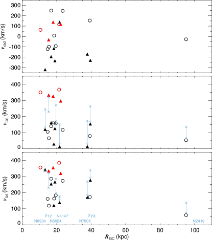
Figure 3: Galactocentric radial (top), tangential (middle), and total velocities (bottom) versus Galactocentric distance of our target GCs. GCs that belong to the young (old) group as listed in Table 1 are plotted as closed triangles (open circles). The five GCs with $v_{\mathrm{tan}}>295$ km s^-1 are plotted in red, while all other GCs are plotted in black to highlight the dichotomy seen in the $v_{\mathrm{tan}}$ distribution. In the middle and bottom panels, velocities implied from the older PM measurements are plotted as light blue $\times$ symbols with arrows pointing to the new measurements for NGC 6934, Pal 12, NGC 5024, NGC 4147, NGC 7006, Pyxis, and NGC 2419 (from left to right as indicated in the bottom panel).

Figure 3 shows the Galacticentric velocities ($v_{\mathrm{rad}}$, $v_{\mathrm{tan}}$, and $v_{\mathrm{tot}}$ taken from Table 4) as a function of distance from the Galactic Center ($R_{\mathrm{GC}}=\sqrt{X^{2}+Y^{2}+Z^{2}}$) for our target GCs. GCs that belong to different age groups (see Table 1) are plotted in different symbols. Overall, we do not find any systematic difference in the velocity distribution between the young and old GCs.

The $v_{\mathrm{rad}}$ vs. $R_{\mathrm{GC}}$ plot in the top panel shows a hint of the well known trend of decreasing velocity dispersion as a function of Galactocentric distance (see e.g., Figure 2 of Battaglia et al., 2005). In the middle panel of Figure 3, we find a clear dichotomy in $v_{\mathrm{tan}}$ among our sample: five GCs have $v_{\mathrm{tan}}\gtrsim 295$ km s^-1 (red), whereas all other GCs have $v_{\mathrm{tan}}<170$ km s^-1(black). These high $v_{\mathrm{tan}}$ GCs are also among the GCs with highest $v_{\mathrm{tot}}$ (bottom panel). Among the five GCs with high $v_{\mathrm{tan}}$, Arp 2, Terzan 7, and Terzan 8 are known to be associated with the Sgr dSph based on their positional and kinematical properties, and Pal 12 is also known to be a likely candidate (Law & Majewski, 2010a). A detailed analysis testing associations with the Sgr dSph is presented in Section 4.2. The remaining cluster, NGC 6101 (which is not associated with the Sgr dSph), has $v_{\mathrm{tan}}\simeq 350$ km s^-1which is comparable to those of Sgr clusters, but very high compared to other halo GCs in our sample. Based purely on the high $v_{\mathrm{tan}}$ and $v_{\mathrm{tot}}$ of this cluster compared to other halo GCs, we propose that NGC 6101 has an origin outside the MW, like the Sgr GCs. Indeed, (Martin et al., 2004) pointed out a possibility that NGC 6101 may be associated with the CMa overdensity.

In the middle and bottom panels of Figure 3, we have included $v_{\mathrm{tan}}$ and $v_{\mathrm{tot}}$ based on the older PM measurements in Table 3 to demonstrate how the Galactocentric velocities change when different PM measurements are adopted. For all but Pal 12, the older PMs implies significantly higher $v_{\mathrm{tan}}$ than those for our HST measurements. This is likely due to the nature of PM measurements in the sense that when systematic uncertainties dominate, there is a tendency of overestimating the measurement therefore yielding higher-than-real energy orbits. A larger PM generally translates to a higher $v_{\mathrm{tan}}$, and as a result, the $v_{\mathrm{tot}}$ is overestimated (see lower panel of Figure 3). For example, based on their PM measurements for NGC 7006, Dinescu et al. (2001) concluded that this cluster is on a highly energetic orbit with the apocentric distance reaching beyond $R_{\mathrm{GC}}=100$ kpc. However, our new PM results imply that NGC 7006 is on an orbit with much lower energy. The most distant cluster in our sample, NGC 2419, also seems to be on a less energetic orbit than implied by the PM measurement by Massari et al. (2017).

4.2 Globular Clusters Associated with the Sagittarius dSph/Stream

We now focus on GCs that have been claimed to be associated with the Sgr Stream, and illustrate how the PM results can aid in the identification. Comprehensive analyses of GCs possibly associated with the Sgr dSph were first performed by Palma et al. (2002) and Bellazzini et al. (2003). Later, Law & Majewski (2010a) carried out a nearly complete census of Sgr GCs by comparing the $N$-body model of the Sgr stream (Law & Majewski, 2010b) to observed parameters (positions, distances, $v_{\mathrm{LOS}}$, and PMs) of GCs residing in the MW halo. They concluded that Arp 2, M54, NGC 5634, Terzan 8, and Whiting 1 are high-probable members of the Sgr dSph, and Berkeley 29, NGC 5053, Pal 12, and Terzan 7 are also likely to be associated with Sgr. Some of the clusters discussed in these papers are included in our sample, so we revisit their identification using our new PM measurements.

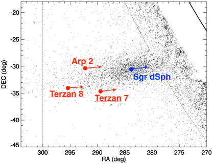
Figure 4: Solar motion-corrected PMs of clusters associated with the Sgr dSph (red arrows), and the Sgr dSph itself (blue arrow). For the blue arrow, we used the perspective-corrected center of mass (COM) motion of $(\mu_{\mathrm{W}},\mu_{\mathrm{N}})=(2.82,-1.51)\,\mathrm{mas}\,\mathrm{yr}^{-1}$ by Sohn et al. (2015). For the solar motion correction of PMs, we assumed the heliocentric distances $D_{\sun}$ listed in Table 4, and for the Sgr dSph $D_{\sun}=28$ kpc. Black dots are the Sgr dSph and stream M-giant stars selected using the 2MASS catalog by Majewski et al. (2003). The relative magnitude of each vector represent the actual difference in space velocity of each component. The dashed lines indicate the region used by Majewski et al. (2003) to fit King profiles to the M-dwarf star counts. The solid line on the upper right marks the Galactic midplane.

Among the clusters we measured PMs for, Arp 2, Terzan 7, and Terzan 8 are the three GCs that are located closest to the Sgr dSph on the sky. These clusters have been associated with the Sgr dSph since the discovery of the dwarf galaxy itself primarily based on their proximities to the dSph’s core (Ibata et al., 1994). Our PMs allow us to compare the motions between these clusters and the Sgr dSph on the sky as illustrated in Figure 4. The vector directions and lengths of the three GCs in Figure 4 agree with those of the Sgr dSph within 3° and $0.33\,\mathrm{mas}\,\mathrm{yr}^{-1}$ (44 km s^-1 at the Sgr dSph distance of 28 kpc), respectively. We therefore conclude that the solar motion-corrected PMs of Arp 2, Terzan 7, and Terzan 8 are consistent with that of the Sgr dSph, which confirms the association.

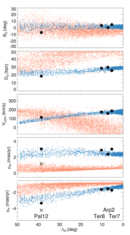
Figure 5: Comparison of observed positions, distances, radial velocities (as measured from the Galactic Standard of Rest or GSR), and PMs (top to bottom) between Pal 12, Terzan 8, Arp 2, and Terzan 7 (black circles) and $N$-body particles of Law & Majewski (2010a) model (red and blue dots). Cluster identifications are labeled in the bottom panel. For Pal 12, we also plot the old PM results of Dinescu et al. (2000) in x symbols. $(\Lambda_{\odot},B_{\odot})$ is the coordinate system as defined by Majewski et al. (2003) that runs along and across the Sgr stream. Coloring scheme of the model particles in this and Figure 6 are the same as in Figure 7 of Sohn et al. (2015): light red and dark blue dots indicate particles on the secondary leading and primary trailing arms, respectively.

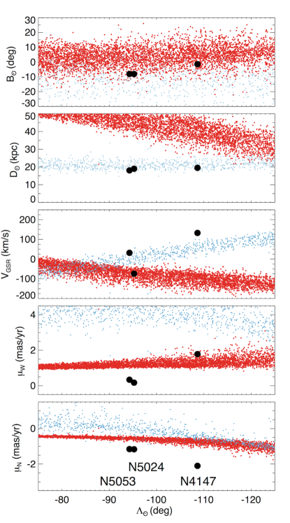
Figure 6: Same as in Figure 5, but for NGC 5053, NGC 5024, and NGC 4147. Dark red and light blue dots indicate model particles on the primary leading and secondary trailing arms, respectively.

Pal 12 has also been suggested as a cluster associated with the Sgr dSph based on its observed parameters (see Law & Majewski, 2010b, and references therein). In Section 4.1, we showed that Pal 12 belongs to the group with higher $v_{\mathrm{tan}}$ among our sample, together with Arp 2, Terzan 7, and Terzan 8, hinting that this cluster is associated with the Sgr dSph. In Figure 5, we provide a more detailed analysis by comparing our results to the $N$-body models of Law & Majewski (2010b). We first note that all observed parameters of Arp 2, Terzan 7, and Terzan 8 indicate that these three clusters follow the motion on the sky of the Sgr trailing arm (as seen in Figure 4). For Pal 12, the position, distance, and radial velocity (top three panels) do not make it clear whether this cluster follows the trailing- (blue) or leading-arm (red) model particles due to the overlap of phase-space information for the two tidal arms in these coordinates. The $N$-body model separates the two tidal arms better in the PM vs. $\Lambda_{\odot}$ phase-space (bottom two panels). Nevertheless, our new PMs make clear that Pal 12 follows the primary Sgr trailing arm debris, at least for this model of the stream. We conclude that Pal 12 is associated with the Sgr dSph, and probably has been brought in together with other Sgr clusters. Our results put to rest contradictory results based on old PM measurements (Dinescu et al., 2000, x symbols) regarding this issue.

In addition to the four Sgr clusters discussed above, NGC 4147, NGC 5024, and NGC 5053 have also been discussed as GCs possibly associated with the Sgr dSph (Law & Majewski, 2010b). We repeat the analysis above for these three clusters and show the results in Figure 6. The position, distance, and radial velocities (top three panels) all indicate a possible connection to the Sgr trailing arm. However, our PM results completely rule out associations with the Sgr dSph. We note that the recent study by Tang et al. (2018) also rules out NGC 5053 Sgr association based on its chemical composition and orbital characteristics.

Finally, NGC 2419 has also been suggested as a cluster associated with the Sgr stream (Newberg et al., 2003; Belokurov et al., 2014). However, this cluster is located in a region where the Law & Majewski (2010b) model is a poor fit to the observed Sgr stream distance, so we cannot use this $N$-body model as a reference here. Instead, we use the observed characteristics of the stream to check whether NGC 2419 is associated. Belokurov et al. (2014) already showed that NGC 2419 is consistent with the sky position, distance, and $v_{\mathrm{LOS}}$ of the trailing arm. The RR Lyrae sample of Sesar et al. (2017) and Hernitschek et al. (2017) show that at this longitude, the trailing arm splits into two components. The denser inner component is centered on $91$ kpc with a width of $7$ kpc, while the lower-density outer component spans roughly 105–120 kpc (Hernitschek et al., 2017). The distance $87.5\pm 3.3$ kpc of di Criscienzo et al. (2011) places NGC 2419 in the inner component. At a distance this large, the density of the general GC population is quite low and a chance coincidence in all these variables is extremely unlikely. Our PM results offer a chance to revisit this assessment.

To explore this in detail, we convert the Galactocentric space motion of NGC 2419 into that of the Sgr coordinate system defined by Majewski et al. (2003). Expressed in spherical coordinates, the radial velocity is $v_{\mathrm{rad}}=-28\pm 1.4$ km s^-1, the azimuthal velocity (along the longitude direction $\Lambda$) is $v_{\mathrm{azi}}=-31\pm 13$ km s^-1, and the polar velocity (in the latitude direction $B$) is $v_{\mathrm{polar}}-43\pm 16$ km s^-1. Here the negative sign on the azimuthal velocity indicates agreement with the orbital direction of the Sgr galaxy and its stream. For comparison, the angular momentum of Sgr itself around the pole of its coordinate system is approximately $L_{z}=-5400$ kpc km s^-1, derived based on the COM PM of the Sgr dSph of Sohn et al. (2015). We expect the angular momentum of stream material to be roughly comparable (though not quite equal) to that of Sgr, so the expected tangential velocity at the cluster’s Galactocentric radius $r\approx 95$ kpc is roughly $v_{\mathrm{tan,s}}\approx-57$ km s^-1. The observed velocity dispersion in the stream is about $\sigma_{\mathrm{intr}}=13$ km s^-1 (Gibbons et al., 2017), which we take as typical even though the dispersion for a globular cluster in the stream at NGC 2419’s location could be somewhat different. Combining the observational error and intrinsic velocity dispersion, the longitudinal motion appears quite consistent with membership in the stream. The motion of NGC 2419 in the polar direction (transverse to the stream path on the sky) of $-43$ km s^-1 is however somewhat surprising in that it is not centered on zero as we might expect. The vast majority of orbits allowed by our measurement put the cluster moving toward the northern Sgr coordinate pole, while a mere 0.4% of the orbits have the opposite sign. Another way to quantify this is the distribution of the orbital poles for this cluster. The angular offset of the pole from that of the Sgr galaxy is $54\pm 16\arcdeg$. Given the $\sim 10\arcdeg$ offset of NGC 2419 from the plane, it is not surprising that there is some offset, but it seems surprisingly large. We intend to investigate this issue further in a future work.

In any case, from a broader perspective, we see that both PM dimensions show agreement with the expected velocities of the Sgr stream material within a few tens of km s^-1. The level of agreement expected from a random coincidence is instead of the order $\sigma_{h}\simeq 120$ km s^-1, the velocity dispersion of the diffuse halo component. We can compute a formal Bayes factor $P_{s}(D)/P_{h}(D)$ representing the relative probability of the observed data with models where NGC 2419 comes from stream and smooth halo components respectively. We fold the observed and intrinsic dispersions together into a total dispersion $\sigma^{\prime}=(\sigma^{2}+\sigma_{\mathrm{intr}})^{1/2}$, and assume normal distributions to get

$$P_{s}(D)=\mathcal{N}(v_{\mathrm{azi}}-v_{\mathrm{azi,s}},\sigma_{\mathrm{azi}}^{\prime 2})\mathcal{N}(v_{\mathrm{polar}},\sigma_{\mathrm{polar}}^{\prime 2})\;,$$ (2)

$$P_{h}(D)=\mathcal{N}(v_{\mathrm{azi}},\sigma_{h}^{\prime 2})\mathcal{N}(v_{\mathrm{polar}},\sigma_{h}^{\prime 2})$$ (3)

For the values given above we find $P_{s}(D)/P_{h}(D)\approx 2$. The somewhat surprising value of the polar velocity is outweighed by the fact we found values somewhat close to expectations for the stream, when for a halo population they did not have to be. The prior odds based on the cluster’s sky position, distance, and radial velocity already favored an association with the stream. Our PM results appear to confirm this association.

4.3 Orbital Parameters

To better understand the origin of our target GCs, we carried out orbital integrations based on our PM measurements. This was done using the code galpy (Bovy, 2015). For the MW potential, we created our own model that is consistent with our MW mass estimated in Section 5.5. We rescaled the NFW halo of mwpotential2014 (included as the default potential in galpy) such that the enclosed mass at $R=250$ kpc is $1.5\times 10^{12}\,\mathrm{M}_{\odot}$. Since our target GCs spend most of their time in the halo, scaling the bulge and disk was not necessary. Adopting a critical overdensity of 100 and the Planck Collaboration et al. (2016) cosmological parameters, the corresponding virial mass of our MW model is $M_{\mathrm{vir}}=1.7\times 10^{12}\,\mathrm{M}_{\odot}$, which is consistent with what we derive in Section 5.5. For the position and velocity of the Sun, we used the same values as in Section 4.1. For better sampling the orbital parameters, we integrated orbits of each cluster backward in time for a duration of 7.5 times its orbital period using the observed positions and velocities as initial conditions. We measured a set of orbital parameters based on this integration span. To calculate uncertainties of each orbital parameter, the process above was repeated using 10,000 Monte Carlo drawings for each GC that samples the observational uncertainties. We note that our uncertainties do not account for the systematics arising from different choice of potentials. Table 5 lists the orbital parameters and associated 1$\sigma$ uncertainties as calculated above for each GC in the following order: total energy, angular momentum in the $Z$-axis direction, magnitude of the angular momentum, pericenter, apocenter, and orbital period.

Table 5: Orbital parameters

	$E_{\mathrm{tot}}$	$L_{Z}$	$|L|$	$R_{\mathrm{peri}}$	$R_{\mathrm{apo}}$	$P$
Cluster	($10^{4}$ km2 s-2)	($10^{3}$ kpc km s-1)	($10^{3}$ kpc km s-1)	(kpc)	(kpc)	(Gyr)
Arp 2	0$-9.1\pm 0.4$	+$1.7\pm 0.2$	$6.6\pm 0.3$	$19.2\pm 0.9$	$49.3\pm$0$5.3$	$0.69\pm 0.07$
IC 4499	$-12.5\pm 0.2$	$-1.2\pm 0.1$	$2.7\pm 0.1$	0$6.3\pm 0.4$	$27.6\pm$0$1.2$	$0.33\pm 0.02$
NGC 1261	$-14.5\pm 0.1$	$-0.4\pm 0.1$	$0.5\pm 0.1$	0$1.1\pm 0.3$	$20.9\pm$0$0.5$	$0.22\pm 0.01$
NGC 2298	$-15.5\pm 0.1$	$-0.5\pm 0.1$	$1.0\pm 0.1$	0$1.3\pm 0.3$	$17.1\pm$0$0.4$	$0.18\pm 0.00$
NGC 2419	0$-6.8\pm 0.1$	+$4.2\pm 1.4$	$5.1\pm 1.2$	$10.5\pm 3.9$	$96.1\pm$0$3.3$	$1.20\pm 0.05$
NGC 4147	$-13.3\pm 0.1$	$-0.1\pm 0.1$	$0.3\pm 0.1$	0$0.4\pm 0.3$	$25.9\pm$0$0.5$	$0.28\pm 0.01$
NGC 5024	$-13.2\pm 0.2$	+$0.8\pm 0.1$	$3.1\pm 0.2$	0$9.1\pm 0.7$	$22.3\pm$0$0.5$	$0.30\pm 0.01$
NGC 5053	$-13.8\pm 0.2$	+$0.7\pm 0.1$	$3.0\pm 0.1$	0$9.9\pm 0.8$	$18.5\pm$0$0.4$	$0.27\pm 0.01$
NGC 5466	$-11.5\pm 0.3$	$-0.8\pm 0.1$	$2.4\pm 0.2$	0$5.3\pm 0.6$	$34.6\pm$0$1.9$	$0.40\pm 0.03$
NGC 6101	$-12.0\pm 0.3$	$-2.9\pm 0.1$	$3.7\pm 0.1$	$10.3\pm 0.2$	$28.2\pm$0$1.5$	$0.37\pm 0.02$
NGC 6426	$-15.2\pm 0.3$	+$1.4\pm 0.2$	$1.6\pm 0.2$	0$3.8\pm 0.6$	$17.3\pm$0$0.8$	$0.20\pm 0.01$
NGC 6934	$-11.2\pm 0.4$	+$1.5\pm 0.2$	$1.6\pm 0.2$	0$3.1\pm 0.4$	$38.0\pm$0$3.0$	$0.42\pm 0.04$
NGC 7006	0$-9.9\pm 0.2$	$-0.5\pm 0.5$	$0.5\pm 0.4$	0$1.0\pm 0.8$	$50.3\pm$0$1.7$	$0.55\pm 0.02$
Pal 12	$-10.6\pm 0.4$	+$2.0\pm 0.1$	$5.1\pm 0.2$	$15.2\pm 0.4$	$36.0\pm$0$3.4$	$0.49\pm 0.04$
Pal 13	$-10.1\pm 0.2$	$-0.8\pm 0.2$	$2.8\pm 0.2$	0$5.6\pm 0.5$	$46.1\pm$0$2.2$	$0.53\pm 0.03$
Pal 15	0$-9.6\pm 0.2$	$-1.3\pm 0.8$	$3.1\pm 0.7$	0$6.3\pm 2.1$	$50.9\pm$0$1.6$	$0.59\pm 0.03$
Pyxis	0$-7.3\pm 0.4$	$-2.0\pm 0.7$	$6.1\pm 0.6$	$13.8\pm 2.0$	$83.7\pm$0$7.4$	$1.06\pm 0.11$
Rup 106	$-11.6\pm 0.2$	+$1.5\pm 0.1$	$2.4\pm 0.1$	0$4.7\pm 0.4$	$34.7\pm$0$1.4$	$0.39\pm 0.02$
Terzan 7	0$-9.1\pm 0.5$	+$1.2\pm 0.2$	$5.9\pm 0.3$	$15.5\pm 0.7$	$51.8\pm$0$5.9$	$0.68\pm 0.08$
Terzan 8	0$-7.0\pm 0.6$	+$1.7\pm 0.3$	$7.9\pm 0.4$	$19.9\pm 0.7$	$87.3\pm$ $14.7$	$1.17\pm 0.21$

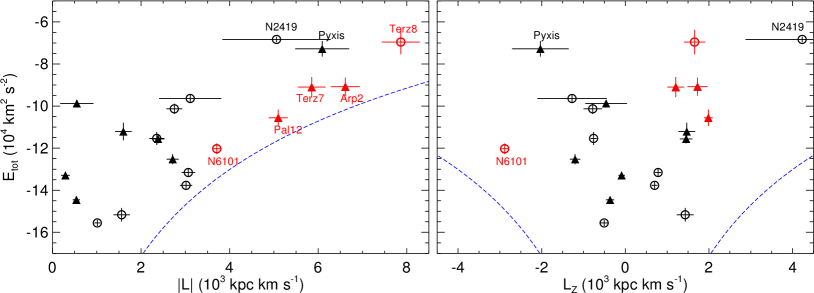
Figure 7: Total orbital energy as a function of the magnitude angular momentum $|L|$ (left panel), and angular momentum in the $Z$-axis direction $L_{\mathrm{Z}}$ (right panel). As in Figure 3, young and old GCs are plotted in closed triangles and open circles, respectively. Also, GCs with $v_{\mathrm{tan}}>290$ km s^-1are plotted in red, while all other GCs are plotted in black. The blue dashed lines indicate the maximum angular momentum allowed by the potential for a given orbital energy. Uncertainties of all parameters plotted here and in Figure 8 were propagated by sampling the observed uncertainties in a Monte Carlo fashion, and do not include the uncertainty in the MW mass model.

Figure 7 shows the total orbital energy as a function of angular momentum. Although the sample is small, the young GCs in the left panel appear to fall into two groups: one group lies at higher energy and angular momentum; and another group lies at low angular momentum, even lower than the older GCs at similar orbital energy range. The separation of these two groups likely indicates that different formation mechanisms exist among the young GCs, e.g., accreted (higher angular momentum) versus within the MW (lower angular momentum). Pyxis is part of the high energy, high angular momentum group, which suggests an external origin (see a detailed discussion in Fritz et al., 2017). From the right panel of Figure 7, we can infer that NGC 6101 has a strong retrograde motion with respect to the rotational direction of the Galactic disk. This strengthens our claim in Section 4.1 that this cluster has an external origin.

In Figure 8, we plot the apocenter versus pericenter of our target GCs. Overall, we find that GCs with $R_{\mathrm{peri}}\lesssim 10$ kpc have orbits only going out to $R_{\mathrm{apo}}\simeq 50$ kpc, while those with $R_{\mathrm{peri}}\gtrsim 10$ kpc have apocenter in the range $30<R_{\mathrm{apo}}<100$ kpc. Related to the two groups of young GCs in the left panel of Figure 7, the GCs in the low energy, low angular momentum have smaller pericenters than the older GCs at similar apocenter range. Among the Sgr GCs, Arp 2, Terzan 7, and Pal 12 (three red triangles) have similar orbital eccentricities of $e\sim 0.5$, whereas the orbit of Terzan 8 is significantly more radial at $e=0.63\pm 0.06$ with the apocenter extending out to $R_{\mathrm{apo}}\sim 90$ kpc. Interestingly, Terzan 8 has been established as being older and more metal-poor than the other Sgr GCs (Montegriffo et al., 1998; Marín-Franch et al., 2009), which suggests that this cluster may have a distinct formation history. The 3D geometry of the Sgr stream recently presented by Belokurov et al. (2014) using blue-HB stars, and later confirmed by Sesar et al. (2017) and Hernitschek et al. (2017) using RR Lyrae stars, reveals that the trailing arm extends out to an extreme distance of $R_{\mathrm{GC}}\sim 100$ kpc. The apocenter of Terzan 8 coinciding with the distance of this extension suggests that this cluster will eventually reside among the extreme trailing debris.

We note that Pal 12 has the lowest apocenter of the Sgr-associated clusters at only $R_{\mathrm{apo}}=36\pm 3$ kpc, despite our earlier conclusion based on comparison to the Law & Majewski (2010b) stream model that it belongs to the trailing stream, which is composed of objects with high energies and apocenters. This puzzle may be resulting from the mismatch between the potential we used for the orbital integrations and that employed for the Law & Majewski model of the stream. As Pal 12 is very near pericenter, its calculated apocenter is maximally sensitive to the potential. Alternatively, Pal 12 could be a member of the leading stream if the actual stream deviates from the Law & Majewski model in this region, which is wrapped $320\arcdeg$ around the sky from Sgr. PMs along the Sgr stream derived from future Gaia data may provide a more robust way of assessing membership in the leading and trailing arms of the stream. All in all, the orbital properties of the Sgr GCs will help constrain the models of Sgr disruption.

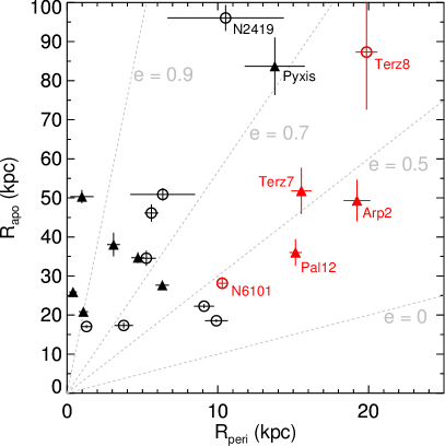
Figure 8: Apocentric versus pericentric distances of our target GCs. Orbital eccentricities of 0, 0.5, 0.7, and 0.9 are plotted as gray dashed lines. For each GC, we used the same symbols and colors as in Figure 3.

5 Mass of the Milky Way using Globular Clusters as Dynamical Tracers

5.1 Method

Traditionally, the spherical Jeans equation (Binney & Tremaine, 2008) has been applied to dynamical tracers to estimate the total MW mass enclosed within a certain radius. Watkins et al. (2010) introduced a variety of mass estimators based on this Jeans equation that work with different types of distance and velocity data depending on which observed parameters are available. Since we have the full 6D phase-space information of our cluster sample, we adopt the estimator that uses intrinsic distances and total velocities. This is written as

$$M\left(<r_{\mathrm{max}}\right)=\frac{1}{G}\frac{\alpha+\gamma-2\beta}{3-2\beta}r_{\mathrm{max}}^{1-\alpha}\left\langle v^{2}r^{\alpha}\right\rangle.$$ (4)

where $r_{\mathrm{max}}$ is the Galactocentric distance of the most distant tracer object, $\alpha$ is the power-law index for the underlying potential ($\Phi\propto r^{-\alpha}$), $\gamma$ is the power-law index for the radial number density profile ($\rho\propto r^{-\gamma}$), and $\beta$ is the velocity anisotropy parameter of the tracer objects. In this section, we calculate these parameters and provide our best estimate of the MW mass using Equation 4.

5.2 Anisotropy Parameter

The anisotropy parameter is defined as

$$\beta\equiv 1-\frac{\sigma_{\theta}^{2}+\sigma_{\phi}^{2}}{2\sigma_{r}^{2}},$$ (5)

where $\sigma_{r}$, $\sigma_{\theta}$, and $\sigma_{\phi}$ denote the velocity dispersions in the radial, polar, and azimuthal directions in spherical coordinates. In general, $\beta$ has been the limiting factor for mass estimations due to the lack of tangential velocities, but our PMs of GCs combined with existing $v_{\mathrm{LOS}}$ allows us to directly calculate $\beta$. To do this, we first consider all GCs in our sample except for NGC 2419. The majority of our cluster sample lie between 10 and 40 kpc, however, NGC 2419 is considerably more distant at $\sim$95 kpc. To first order, $M\propto v^{2}r$, so points at large $r$ have the most weight in the mass estimate; this makes it particularly important that the RMS velocity is accurately estimated at large distance, and this cannot be guaranteed when there is only a single tracer. Were we to include NGC 2419 in the following analysis, there is a risk that our mass estimate would be significantly biased by the presence of this single cluster at a distance far greater than the others. As such, we remove this cluster from our sample in subsequent analyses.

Table 6: Velocity mean, dispersions, and anisotropy parameters

		$\overline{v_{r}}$	$\overline{v_{\theta}}$	$\overline{v_{\phi}}$	$\sigma_{r}$	$\sigma_{\theta}$	$\sigma_{\phi}$
	$N_{\mathrm{sample}}$	(km s-1)	(km s-1)	(km s-1)	(km s-1)	(km s-1)	(km s-1)	$\beta$
Sample1	19	$-20.2\pm 39.3$	$-65.9\pm 36.0$	$-21.5\pm 29.1$	$171.1\pm 27.3$	$156.7\pm 25.5$	$126.2\pm 20.2$	$0.309\begin{subarray}{c}+0.213\\ -0.377\end{subarray}$
Sample2	16	$-37.9\pm 45.3$	$-26.2\pm 28.6$	+0$3.3\pm 28.2$	$181.1\pm 32.0$	$114.0\pm 20.0$	$112.3\pm 20.1$	$0.609\begin{subarray}{c}+0.130\\ -0.229\end{subarray}$

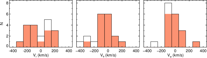
Figure 9: Histogram of spherical velocity components for Sample1 (black outline) and Sample2 (red blocks) as defined in Table 6.

We converted the space velocities in the Cartesian coordinate system $(v_{X},\,v_{Y},\,v_{Z})$ of our GCs as listed in Table 4 to velocities in the spherical coordinate system $(v_{r},\,v_{\theta},\,v_{\phi})$. We then calculated the mean velocities $(\overline{v_{r}},\,\overline{v_{\theta}},\,\overline{v_{\phi}})$, velocity dispersions $(\sigma_{r},\,\sigma_{\theta},\,\sigma_{\phi})$, and the resulting velocity anisotropy parameter $\beta$. The uncertainties were calculated using the maximum likelihood estimation method assuming the uncertainty distribution in each coordinate is Gaussian. Results for the 19 GCs (excluding NGC 2419) are shown in Table 6 (Sample1), and the distribution of each velocity component is plotted in Figure 9.

For a pressure-supported system such as the halo GCs, one expects the mean velocity of each component to be zero. This is the case for the mean radial ($\overline{v_{r}}$) and azimuthal velocities ($\overline{v_{\phi}}$), but we find that the mean polar velocity is non-zero at $\sim 2\sigma$ level ($\overline{v_{\theta}}=-65.9\pm 35.9$ km s^-1). Figure 9 indeed shows an excess in negative $v_{\theta}$. As discussed in Section 4.2, our sample contains four Sgr clusters. The Sgr dSph is known to have a nearly polar orbit about the MW disk, and so the non-zero mean polar velocity (i.e., motion in vertical direction w.r.t. the disk) for Sample1 is likely due to the presence of Sgr GCs. This indicates that Sample1 does not correctly represent the halo GC population, and using this sample will significantly bias our mass estimates. There are at least 5 confirmed Sgr GCs (Arp 2, Terzan 7, Terzan 8, Pal 12 analyzed in this study, and M54 which resides near the core of the Sgr dSph; Bellazzini et al., 2008), so one out of every $\sim 20$ halo GCs is associated with the Sgr dSph. As such, to correctly represent the halo GC population, we decided to exclude three of the four Sgr GCs from our sample, keeping only Arp 2. We denote this as Sample2 and repeat the calculations above. Results are shown in the second row of Table 6, and we now find that the mean velocities of all three components are consistent with zero. Our final anisotropy parameter adopted for the purpose of MW mass calculations below is $\beta=0.609\begin{subarray}{c}+0.130\\ -0.229\end{subarray}$.

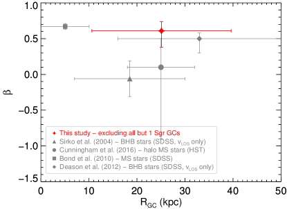
Figure 10: Velocity anisotropy profile of the MW halo.

Figure 10 shows our anisotropy parameter for GCs compared to those calculated from other studies using halo stars in the range $0<R_{\mathrm{GC}}<50$ kpc. Our $\beta$ implies more radially-biased orbital motions than the results of Sirko et al. (2004) and Cunningham et al. (2016) in a similar $R_{\mathrm{GC}}$ range. Sirko et al. (2004) used a large sample of SDSS halo stars spread across a significant portion of the sky, but only used $v_{\mathrm{LOS}}$ to constrain $\beta$. However, as shown by Hattori et al. (2017), measurements of $\beta$ from $v_{\mathrm{LOS}}$ alone can be unreliable beyond $R_{\mathrm{GC}}\sim 15$ kpc. On the other hand, while Cunningham et al. (2016) used PMs of halo stars measured via HST, their measurement is confined to a single line-of-sight, and is likely the result of including stars in a large shell-type structure such as the “TriAnd” overdensity, and therefore may not represent the relaxed halo system. If our $\beta$ from GCs represents the underlying halo system in the distance range $R_{\mathrm{GC}}=10-40$, the “dip” observed by Cunningham et al. (2016) can be interpreted as being a localized effect rather than a global decrease in $\beta$.

Our $\beta$ comfortably lies between those measured using stars in solar neighborhood (Bond et al., 2010), and distant halo stars (Deason et al., 2012) (although the latter also potentially suffers from using only $v_{\mathrm{LOS}}$). Furthermore, the $\beta$ we measure for the halo GCs is in good agreement with simulations of stellar haloes, which generally predict radially anisotropic orbits at large distances (Diemand et al., 2007; Rashkov et al., 2013; Loebman et al., 2018).

5.3 Density and Potential

For the density slope, we use $\gamma=3.53\pm 0.01$, which we find by fitting to the halo clusters in the H10 catalog, and is in good agreement with previous values quoted in the literature (e.g. Harris, 2001). This we henceforth consider to be fixed. For the mass estimates, we will use Sample2, that is the sample with NGC 2419, Terzan 7, Terzan 8 and Pal 12 excluded. These clusters span $10.6\leq r\leq 39.5$ kpc, so we need to estimate the slope of underlying potential over this radial range. To do this, we consider a set of MW models for which the nucleus, bulge, and disk components are fixed, but the properties of the halo are allowed to vary – we assume the halo is NFW (Navarro et al., 1996) in shape but vary both the mass and scale radius. The halos are further chosen to be consistent with both existing literature on theoretical MW potential profiles and the observed solar velocity. The resulting distribution of $\alpha$ spans approximately $0.21\lesssim\alpha\lesssim 0.52$. Both the density- and potential-fitting methods are described in detail in Watkins & van der Marel (2018) and are similar to the methods used in Annibali et al. (2018).

5.4 Monte Carlo Simulations

We also need to consider the shot noise in our calculations, that is how well the mass estimated using our sample of 16 clusters describes the underlying mass distribution from which they were drawn. In Watkins et al. (2010), we describe a suite of Monte Carlo simulations that were created for this purpose. We run 1000 simulations of 16 clusters, and calculate the mass in each case. Reassuringly, we find that the the fraction $f=M_{\mathrm{est}}/M_{\mathrm{true}}$ of the estimated mass to the true mass is $f=1.00\pm 0.22$, so our estimators do indeed recover the true mass on average. Further, we can use these simulations to provide accurate error bars on our mass estimates that correctly account for shot noise.

5.5 Milky Way Mass

Now that we have the ingredients in place, we proceed with estimating the mass of the MW within $r_{\mathrm{max}}=39.5$ kpc. For each of the $\alpha$ values obtained from our model halos, we draw an anisotropy $\beta$ at random from the posterior distribution for the fit in Section 5.2 and calculate the mass $M\left(<r_{\mathrm{max}}\right)_{\rm est}$. Then we can infer the true mass $M\left(<r_{\mathrm{max}}\right)$ from this mass estimate by drawing a value of $f$ at random from the Monte Carlo simulation sample. We adopt the median of these masses as the best mass estimate, and use the 1-$\sigma$ (15.9 and 84.1) percentiles to estimate uncertainties. Thus, we estimate the mass of the MW to be

$$M\left(<r_{\mathrm{max}}\right)=0.61\begin{subarray}{c}+0.18\\ -0.12\end{subarray}\times 10^{12}\,\mathrm{M}_{\odot}.$$ (6)

By drawing $f$ and $\beta$ values at random, shot noise and the uncertainties on the anisotropy are naturally folded into our result. From this, we can estimate the circular velocity at $r_{\mathrm{max}}$, for which we find

$$v_{\mathrm{circ}}(r_{\mathrm{max}})=259^{+35}_{-26}\,\mathrm{km\,s}^{-1}.$$ (7)

By comparing $M\left(<r_{\mathrm{max}}\right)$ and the virial mass $M_{\mathrm{vir}}$ for our model halos, we can also infer a virial mass for the MW from our estimate of the mass within $r_{\mathrm{max}}$. Thus we find the virial mass implied by our tracer mass estimates to be

$$M_{\mathrm{vir}}=2.05^{+0.97}_{-0.79}\times 10^{12}\,\mathrm{M}_{\odot}.$$ (8)

Again, the uncertainties on the anisotropy have been propagated into these uncertainties. We note that $M_{\mathrm{vir}}$ has larger fractional uncertainty than $M\left(<r_{\mathrm{max}}\right)$ due to the uncertainty in the extrapolation of the dark halo mass profile to large radii.

6 Conclusions

We present high-precision PM measurements of 20 GCs in the MW halo. The bulk motions of numerous GC stars were compared against distant background galaxies to achieve a median PM uncertainty of $0.06\,\mathrm{mas}\,\mathrm{yr}^{-1}$ per coordinate per cluster. Our PM results are not affected by possible rotation in the plane of the sky, and therefore represents the COM motions. For 10 out of 20 GCs, we compared our new PM results with previous measurements, which have much larger random (and systematic) uncertainties. The new and old results agree within the claimed 1$\sigma$ uncertainties for four of these, while the rest are inconsistent with each other. We also find that the previous PM measurements systematically imply higher $v_{\mathrm{tan}}$ and $v_{\mathrm{tot}}$ (except for one GC we inspected).

We derive space motions of our target GCs in the Galactocentric frame by combining the newly measured PMs with existing $v_{\mathrm{LOS}}$ measurements. We find a clear dichotomy in the Galactocentric $v_{\mathrm{tan}}$ distribution such that there are five GCs with $v_{\mathrm{tan}}>290$ km s^-1 (NGC 6101, Arp 2, Terzan 7, Terzan 8, and Pal 12) while all other GCs have $v_{\mathrm{tan}}<200$ km s^-1. Four of these five GCs with high $v_{\mathrm{tan}}$ are confirmed to be associated with the Sgr dSph based on comparing their observed properties to those of model particles of Law & Majewski (2010a). We have tested the Sgr associations for three other GCs (NGC 4147, NGC 5024, and NGC 5053) and found that they can be ruled out based on our PM measurements. We also discuss the Sgr association of NGC 2419, the most distant cluster in our sample. Our PM implies that NGC 2419 seems to be associated with the Sgr stream debris recently found at distances similar to this cluster. However, we find an interesting offset in motion in the transverse direction with respect to the stream path. We integrate orbits of our target GCs based on our PMs to explore their origins. We find that the young GCs can be separated into two groups, one with high orbital energy and angular momentum (which includes the Sgr GCs and Pyxis), and the other with low energy and momentum. This likely indicates two different origins among the young GCs, namely, accreted versus within-MW formation. Terzan 8 which is older and more metal-poor than the other Sgr GCs, is also on a significantly less energetic orbit.

We use a selected sample of GCs from our targets as dynamical tracers to provide a robust estimate of the MW mass. To represent the halo GC population in the range $R_{\mathrm{GC}}=10$–40 kpc, we remove NGC 2419, and include only one out of the four confirmed Sgr cluster. We then calculate the anisotropy parameter for the 16 clusters as $\beta=0.609\begin{subarray}{c}+0.130\\ -0.229\end{subarray}$. This implies significantly more radially-biased orbits than the $\beta$ measured using halo stars in similar Galactocentric distance ranges, which may be due to the fact that the halo star samples are biased by dynamically cold substructures in the halo, and that previous measurements relied on $v_{\mathrm{LOS}}$ alone to compute $\beta$, and this procedure can be unreliable at large Galactocentric distances ($>15$ kpc). We provide estimates of the power indices for the number density profile, as well as the underlying potential and calculate the MW mass using a tracer mass estimator that considers the full 6D phase-space information as inputs. Our best estimate for the MW mass within $R_{\mathrm{GC}}=39.5$ kpc is $M(<39.5~{}\mathrm{kpc})=0.61\begin{subarray}{c}+0.18\\ -0.12\end{subarray}\times 10^{12}\,\mathrm{M}_{\odot}$. We extrapolate our mass estimate to calculate the virial mass to be $M_{\mathrm{vir}}=2.05\begin{subarray}{c}+0.97\\ -0.79\end{subarray}\times 10^{12}\,\mathrm{M}_{\odot}$.

PM measurements using multi-epoch HST data have provided a breakthrough in understanding dynamics of tracer objects in the MW halo. Through our HSTPROMO collaboration (van der Marel et al., 2014), we are continuing to make progress in improving the quality and quantity of PM measurements. While the release of Gaia DR2 (and subsequent data releases) will undoubtedly provide PMs for a wealth of halo objects, PMs with HST will continue to be powerful for distant stellar systems. HST results such as those presented in this paper should also prove to be very useful as an independent check for the upcoming Gaia data releases.

References

- Anderson (2006) Anderson, J., 2006, in The 2005 HST Calibration Workshop, ed., A. M. Koekemoer, P. Goudfrooij, & L. Dressel (Baltimore, MD: STScI), 11
- Anderson & King (2006) Anderson, J., & King, I. R. 2006, ACS/ISR 2006-01, PSFs, Photometry, and Astrometry for the ACS/WFC (Baltimore, MD: STScI)
- Anderson & Bedin (2010) Anderson, J. & Bedin, L. R. 2010, PASP, 122, 1035
- Annibali et al. (2018) Annibali, F., Morandi, E., Watkins, L. L., et al. 2018, MNRAS, arXiv:1802.02338
- Battaglia et al. (2005) Battaglia, G., Helmi, A., Morrison, H., et al. 2005, MNRAS, 364, 433
- Baumgardt et al. (2009) Baumgardt, H., Côté, P., Hilker M., et al. 2009, MNRAS, 396, 2051
- Bellazzini et al. (2003) Bellazzini, M., Ferraro, F. R., Ibata, R. A. 2003, AJ, 125, 188
- Bellazzini et al. (2008) Bellazzini, M., Ibata, R., Chapman, S. C., et al. 2008, AJ, 136, 1147
- Bellini et al. (2011) Bellini, A., Anderson, J., & Bedin, L. R. 2011, PASP, 123, 622
- Bellini et al. (2017) Bellini, A., Bianchini, P., Varri, A. L., et al. 2017, ApJ, 844, 167
- Belokurov et al. (2014) Belokurov, V., Koposov, S. E., Evans, N. W., et al. 2014, MNRAS, 437, 116
- Bertin & Arnouts (1996) Bertin, E., & Arnouts, S. 1996, \aas, 117, 393
- Besla et al. (2007) Besla, G., Kallivayalil, N., Hernquist, L., et al. 2007, ApJ, 668, 949
- Bianchini et al. (2013) Bianchini, P., Varri, A. L., Bertin, G., & Zocchi, A. 2013, ApJ, 772, 67
- Binney & Tremaine (2008) Binney, J., & Tremaine, S. 2008, Galactic Dynamics (Princeton: Princeton Univ. Press)
- Bond et al. (2010) Bond, N. A., Ivezić, Ž, Sesar, B., et al. 2010, ApJ, 716, 1
- Bovy (2015) Bovy, J. 2015, ApJS, 216, 29
- Boylan-Kolchin et al. (2013) Boylan-Kolchin, M., Bullock, J. S., Sohn, S. T., Besla, G., & van der Marel, R. P. 2013, ApJ, 768, 140
- Cunningham et al. (2016) Cunningham, E. C., Deason, A. J., Guhathakurta, P., et al. 2016, ApJ, 820, 18
- Deason et al. (2011) Deason, A. J., McCarthy, I. G., Font, A. S., et al. 2011, MNRAS, 415, 2607
- Deason et al. (2012) Deason, A. J., Belokurov, V., Evans, N. W., & An, J., 2012, MNRAS, 424, L44
- di Criscienzo et al. (2011) di Criscienzo, M., Greco, C., Ripepi, V., et al. 2011, AJ, 141, 81
- Diemand et al. (2007) Diemand, J., Kuhlen, M., & Madau, P. 2007, ApJ, 667, 859
- Dinescu et al. (1999) Dinescu, D. I., van Altena, W. F., & Girrard, T. M. 1999, AJ, 117, 277
- Dinescu et al. (2000) Dinescu, D. I., Majewski, S. R., Girrard, T. M., & Cudworth, K. M. 2000, AJ, 120, 1892
- Dinescu et al. (2001) Dinescu, D. I., Majewski, S. R., Girrard, T. M., & Cudworth, K. M. 2001, AJ, 122, 1916
- Dotter et al. (2010) Dotter, A., Sarajedini, A., & Anderson, J., et al. 2010, ApJ, 708, 698
- Dotter et al. (2011) Dotter, A., Sarajedini, A., & Anderson, J. 2011, ApJ, 738, 74
- Eggen et al. (1962) Eggen, O. J., Lynden-Bell, D., & Sandage, A. R. 1962, ApJ, 136, 748
- Fragione & Leob (2017) Fragione, G., & Loeb, A. 2017, New A, 55, 32
- Fritz et al. (2017) Fritz, T. K., Linden, S. T., Zivick, P., et al. 2017, ApJ, 840, 30
- Gibbons et al. (2017) Gibbons, S. L. J., Belokurov, V., & Evans, N. W. 2017, MNRAS, 464, 794
- Gnedin et al. (2010) Gnedin, O. Y., Brown, W. R., Geller, M. J., & Kenyon, S. J. 2010, ApJ, 720, L108
- Harris (1996) Harris, W. E. 1996, AJ, 112, 1487
- Harris (2001) Harris, W. E. 2001, Globular Cluster Systems, 223
- Hamren et al. (2013) Hamren, K. M., Smith, G. H., Guhathakurta, P., et al. 2013, AJ, 146, 116
- Hanke et al. (2017) Hanke, M., Kock, A., Hanser, C. J., & McWilliam, A. 2017, A&A, 599, A97
- Hankey & Cole (2011) Hankey, W. J., & Cole, A. A. 2011, MNRAS, 411, 1536
- Hattori et al. (2017) Hattori, K., Valluri, M., Loebman, S. R., & Bell, E. F. 2017, ApJ, 841, 91
- Hernitschek et al. (2017) Hernitschek, N., Sesar, B., Rix, H.-W., et al. 2017, ApJ, 850, 96
- Ibata et al. (1994) Ibata, R. A., Gilmore, G., & Irwin, M. J. 1994, Nature, 370, 194
- Kharchenko et al. (2013) Kharchenko, N. V., Piskunov, A. E., Schilbach, E., Röser, S., & Scholz, R.-D. 2013, A&A, 558, A53
- Kimmig et al. (2015) Kimmig, B., Seth, A., Ivans, I. I., et al. 2015, AJ, 149, 53
- King et al. (2015) King, C. III., Brown, W. R., Geller, M. J., & Kenyon, S. J. 2015, ApJ, 813, 89
- Law & Majewski (2010a) Law, D. R., & Majewski, S. R. 2010a, ApJ, 718, 1128
- Law & Majewski (2010b) Law, D. R., & Majewski, S. R. 2010b, ApJ, 714, 229
- Libralato et al. (2018a) Libralato, M., Bellini, A., van der Marel, R. P., et al. 2018a, ApJ, in pess (arXiv:1805.05332)
- Libralato et al. (2018b) Libralato, M., Bellini, A., Bedin, L. R., et al. 2018b, ApJ, 854, 45
- Loebman et al. (2018) Loebman, S. R., Valluri, M., Hattori, K., et al. 2018, ApJ, 853, 196
- Mackey & Gilmore (2004) Mackey, A. D., & Gilmore, G. F. 2004, MNRAS, 355, 504
- Majewski et al. (2003) Majewski, S. R. Skrutskie, M. F., Weinberg, M. D., & Ostheimer, J. C. 2003, ApJ, 599, 1082
- Marín-Franch et al. (2009) Marín-Franch, A., Aparicio, A., Piotto, G., et al. 2009, ApJ, 694, 1498
- Martin et al. (2004) Martin, N. F., Ibata, R. A., Bellazzini, M., et al. 2004, MNRAS, 348, 12
- Massari et al. (2013) Massari, D., Bellini, A., Ferraro, F. R., et al. 2013, ApJ, 779, 81
- Massari et al. (2017) Massari, D., Posti, L., Helmi, A., Fiorentino, G., & Tolstoy, E. 2017, A&A, 598, 9
- McMillan (2011) McMillan, P. J. 2011, MNRAS, 414, 2446
- Miyamoto & Nagai (1975) Miyamoto, M., & Nagai, R. 1975, PASJ, 27, 533
- Montegriffo et al. (1998) Montegriffo, P., Bellazzini, M., Ferraro, F. R., et al. 1998, MNRAS, 294, 315
- Navarro et al. (1996) Navarro, J. F., Frenk, C. S., & White, S. D. M. 1996, ApJ, 462, 563
- Newberg et al. (2003) Newberg, H. J., Yanny, B., Grebel, E. K., et al. 2003, ApJ, 596, L191
- Odenkirchen et al. (1997) Odenkirchen, M., Brosche, P., Geffert, M., & Tucholke, H.-J. 1997, New A, 2, 477
- Palma et al. (2002) Palma, C., Majewski, S. R., & Johnston, K. V. 2002, ApJ, 564, 736
- Patel et al. (2017) Patel, E., Besla, G., & Sohn, S. T. 2017, MNRAS, 464, 3825
- Patel et al. (2018) Patel, E., Besla, G., Mandel, K., & Sohn, S. T. 2018, ApJ, submitted (arXiv:1803.01878)
- Peñarrubia et al. (2016) Peñarrubia, J., Gómez, F. A., Besla, G., Erkal, D., & Ma, Y.-Z. 2016, MNRAS, 456, L54
- Perryman et al. (1997) Perryman, M. A. C., Lindegren, L., Kavlevsky, J., et al. 1997, A&A, 323, L49
- Planck Collaboration et al. (2016) Planck Collaboration et al. 2016, A&A, 594, A13
- Rashkov et al. (2013) Rashkov, V., Pillepich, A., Deason, A. J., et al. 2013, ApJ, 773, L32
- Röser et al. (2010) Röser, S., Demeleitner, M., & Schilbach, E. 2010, AJ, 139, 2440
- Rossi et al. (2017) Rossi, E. M., Marchetti, T., Cacciato, M., Kuiack, M., & Sari, R. MNRAS, 467, 1844
- Sarajedini et al. (2007) Sarajedini, A., Bedin, L. R., Chaboyer, B., et al. 2007, AJ, 133, 1658
- Schlafly & Finkbeiner (2011) Schlafly, E. F., & Finkbeiner, D. P. 2011, ApJ, 737, 103
- Schönrich, Binney, & Dehnen (2010) Schönrich, R., Binney, J., & Dehnen, W. 2010, MNRAS, 403, 1829
- Searle & Zinn (1978) Searle, L., & Zinn, R. 1978, ApJ, 225, 357
- Sesar et al. (2017) Sesar, B., Hernitschek, N., Dierickx, M. I. P., Fardal, M. A., & Rix, H.-W. 2017, ApJ, 844, L4
- Siegel et al. (2001) Siegel, M. H., Majewski, S. R., Cudworth, K. M., & Takamiya, M. 2001, AJ, 121, 935
- Sirko et al. (2004) Sirko, E., Goodman, J., Knapp, G. R., et al. 2004, AJ, 127, 914
- Sollima et al. (2014) Sollima, A., Carretta, E., D’Orazi, V., et al. 2014, MNRAS, 443, 1425
- Sohn et al. (2012) Sohn, S. T., Anderson, J., & van der Marel, R. P. 2012, ApJ, 753, 7
- Sohn et al. (2013) Sohn, S. T., Besla, G., van der Marel, R. P., et al. 2013, ApJ, 768, 139
- Sohn et al. (2015) Sohn, S. T., van der Marel, R. P., Carlin, J. L., et al. 2015, ApJ, 803, 56
- Sohn et al. (2016) Sohn, S. T., van der Marel, R. P., Kallivayalil, N., et al. 2016, ApJ, 833, 235
- Sohn et al. (2017) Sohn, S. T., Patel, E., Besla, G., et al. 2017, ApJ, in press
- Tang et al. (2018) Tang, B., Fernández-Trincado, J. G., Geisler, D., et al. 2018, ApJ, 855, 38
- van der Marel et al. (2012) van der Marel, R. P., Fardal, M., Besla, G., et al. 2012, ApJ, 753, 8
- van der Marel et al. (2014) van der Marel, R. P., Anderson, J., Bellini, A., et al. 2014, in ASP Conf. Ser. 480, Structure and Dynamics of Disk Galaxies, ed. M. S. Seigar & P. Treuthardt (San Francisco, CA: ASP), 43
- Watkins et al. (2010) Watkins, L. L., Evans, N. W., & An, J. H. 2010, MNRAS, 406, 264