Linear-response density cumulant theory for excited electronic states

Abstract

We present a linear-response formulation of density cumulant theory (DCT) that provides a balanced and accurate description of many electronic states simultaneously. In the original DCT formulation, only information about a single electronic state (usually, the ground state) is obtained. We discuss the derivation of linear-response DCT, present its implementation for the ODC-12 method (LR-ODC-12), and benchmark its performance for excitation energies in small molecules (N2, CO, HCN, HNC, C2H2, and H2CO), as well as challenging excited states in ethylene, butadiene, and hexatriene. For small molecules, LR-ODC-12 shows smaller mean absolute errors in excitation energies than equation-of-motion coupled cluster theory with single and double excitations (EOM-CCSD), relative to the reference data from EOM-CCSDT. In a study of butadiene and hexatriene, LR-ODC-12 correctly describes the relative energies of the singly-excited $1{}^{1}\mathrm{B_{u}}$ and the doubly-excited $2{}^{1}\mathrm{A_{g}}$ states, in excellent agreement with highly accurate semistochastic heat-bath configuration interaction results, while EOM-CCSD overestimates the energy of the $2{}^{1}\mathrm{A_{g}}$ state by almost 1 eV. Our results demonstrate that linear-response DCT is a promising theoretical approach for excited states of molecules.

1 Introduction

Accurate simulation of excited electronic states remains one of the major challenges in modern electronic structure theory. Ab initio methods for excited states can be divided into single-reference and multi-reference categories, based on their ability to treat static electron correlation. Multi-reference methods ^{1, 2, 3, 4, 5, 6, 7, 8, 9, 10, 11, 12, 13, 14, 15, 16, 17, 18} can correctly describe static correlation in near-degenerate valence orbitals and electronic states with multiple-excitation character, but often lack accurate treatment of important dynamic correlation effects or become computationally very costly when the number of strongly correlated orbitals is large. Meanwhile, single-reference methods ^{19, 20, 21, 22, 23, 24, 25, 26, 27, 28, 29, 30, 31, 32, 33} often provide a compromise between the computational cost and accuracy, and can be used to reliably compute properties of molecules in low-lying electronic states near the equilibrium geometries. In these situations, single-reference equation-of-motion coupled cluster theory (EOM-CC) ^{21, 22, 23, 24, 25, 26} is usually the method of choice, especially when high accuracy is desired.

The EOM-CC methods yield size-intensive excitation energies ^{28, 29} and can be systematically improved by increasing the excitation rank of the cluster operator in the exponential parametrization of the wavefunction. Although EOM-CC is usually formulated in the context of a similarity-transformed Hamiltonian, its excitation energies are equivalent to those obtained from linear-response coupled cluster theory (LR-CC). ^{27, 28, 29} Both EOM-CC and LR-CC are based on non-Hermitian eigenvalue problems, which complicates the computation of molecular properties (e.g., transition dipoles) by requiring evaluation of left and right eigenvectors, ^{34, 35, 36, 37} and may result in an incorrect description of potential energy surfaces in the vicinity of conical intersections where complex excitation energies may be obtained.^{38, 39, 40} Several Hermitian alternatives to EOM-CC and LR-CC have been proposed to avoid these problems, such as algebraic diagrammatic construction ^{41, 42, 43}, unitary and variational LR-CC, ^{44, 45, 46} similarity-constrained CC, ⁴⁷ and propagator-based LR-CC. ^{48, 49}

In this work, we present a linear-response formulation of density cumulant theory for excited electronic states. In density cumulant theory (DCT), ^{50, 51, 52, 53, 54, 55, 56, 57} the electronic energy is determined directly in terms of the one-particle reduced density matrix and the density cumulant, i.e. the fully connected part of the two-body reduced density matrix (2-RDM). ^{58, 59, 60, 61, 62, 63, 64, 65, 66, 67} In this regard, DCT is related to approaches based on the variational optimization ^{68, 69, 62, 70, 71, 72, 73, 74, 75} or parametrization ^{76, 77, 78} of the 2-RDM. On the other hand, DCT has a close relationship with wavefunction-based electronic structure theories, ^{53, 54} such as linearized, unitary, and variational coupled cluster theory. ^{79, 80, 81, 82, 83, 84, 85, 86, 87} In contrast to variational 2-RDM theory ^{88, 89, 90} and traditional coupled cluster methods,^{25, 26} DCT naturally combines size-extensivity and a Hermitian energy functional. In addition, the DCT electronic energy is fully optimized with respect to all of its parameters, which greatly simplifies computation of the first-order molecular properties. ^{91, 92, 93, 94} We have successfully applied DCT to a variety of chemical systems with different electronic structure effects (e.g., open-shell, symmetry-breaking, and multi-reference). ^{54, 55, 56, 95, 96} One limitation of the original DCT formulation is the ability to describe only the lowest-energy state of a particular symmetry (usually, the ground state). By combining DCT with linear response theory, we remove this limitation, providing access to many electronic states simultaneously.

We begin with a brief overview of DCT (Section 2.1) and linear response theory (Section 2.2). In Section 2.3, we describe the derivation of the linear-response equations for the ODC-12 model (LR-ODC-12). In Section 2.4, we compare the LR-ODC-12 method with linear-response orbital-optimized linearized coupled cluster theory with double excitations (LR-OLCCD), which we derive by linearizing the LR-ODC-12 equations. We outline the computational details in Section 3. In Section 4, we demonstrate that the LR-ODC-12 excitation energies are size-intensive (Section 4.1), test the performance of LR-ODC-12 for the dissociation of H2 (Section 4.2), benchmark its accuracy for vertical excitation energies of small molecules (Section 4.3), and apply LR-ODC-12 to challenging excited states in ethylene, butadiene, and hexatriene (Section 4.4). We present our conclusions in Section 5.

2 Theory

2.1 Overview of Density Cumulant Functional Theory

We begin with a brief overview of density cumulant theory (DCT) for a single electronic state. Our starting point is to express the electronic energy as a trace of the one- and antisymmetrized two-electron integrals ($h_{p}^{q}$ and $\overline{g}_{pq}^{rs}$) with the reduced one- and two-body density matrices ($\gamma^{p}_{q}$ and $\gamma^{pq}_{rs}$):

$$E=h_{p}^{q}\gamma^{p}_{q}+\tfrac{1}{4}\overline{g}_{pq}^{rs}\gamma^{pq}_{rs}$$ (1)

where summation over the repeated indices is implied. In DCT, the two-body density matrix $\gamma^{pq}_{rs}$ is expanded in terms of its connected part, the two-body density cumulant ($\lambda^{pq}_{rs}$), and its disconnected part, which is given by an antisymmetrized product of one-body density matrices:⁵⁰

$$\gamma^{pq}_{rs}=\langle\Psi|a^{pq}_{rs}|\Psi\rangle=\lambda^{pq}_{rs}+P_{(r/s)}\gamma^{p}_{r}\gamma^{q}_{s}$$ (2)

where $P_{(r/s)}v_{rs}=v_{rs}-v_{sr}$ denotes antisymmetrization and $a^{pq}_{rs}=a^{{\dagger}}_{p}a^{{\dagger}}_{q}a_{s}a_{r}$ is the two-body operator in second quantization. The one-body density matrix $\gamma^{p}_{q}$ is determined from its non-linear relationship to the cumulant’s partial trace:⁵³

$$\gamma^{p}_{q}=\gamma^{p}_{r}\gamma^{r}_{q}-\lambda^{pr}_{qr}$$ (3)

This allows us to determine the energy (1) from the two-body density cumulant and the spin-orbitals, thereby defining the DCT energy functional. The density cumulant is parametrized by choosing a specific Ansatz for the wavefunction $|\Psi\rangle$ such that⁵⁵

$$\lambda^{pq}_{rs}=\langle\Psi|a^{pq}_{rs}|\Psi\rangle_{c}$$ (4)

where $c$ indicates that only fully connected terms are included in the parametrization. Importantly, due to the connected nature of Eq. 4, DCT is both size-consistent and size-extensive for any parametrization of $|\Psi\rangle$, and is exact in the limit of a complete parametrization (i.e., when $|\Psi\rangle$ is expanded in the full Hilbert space).⁵⁵ Eq. 4 can be considered as a set of $n$-representability conditions that constrain the resulting one- and two-body density matrices to (at least approximately) represent a physical $n$-electron wavefunction. To compute the DCT energy, the functional (1) is made stationary with respect to all of its parameters.

In this work, we consider the ODC-12 method,^{53, 54} which uses an approximate parametrization for the cumulant in Eq. 4 where the wavefunction $\ket{\Psi}$ is expressed using a unitary transformation truncated at the second order:⁵⁵

$$\lambda^{pq}_{rs} \approx\langle\Phi|e^{-(\hat{T}_{2}-\hat{T}^{\dagger}_{2})}a^{pq}_{rs}e^{\hat{T}_{2}-\hat{T}^{\dagger}_{2}}|\Phi\rangle_{c}$$

$$\approx\langle\Phi|a^{pq}_{rs}|\Phi\rangle_{c}+\langle\Phi|[a^{pq}_{rs},\hat{T}_{2}-\hat{T}^{\dagger}_{2}]|\Phi\rangle_{c}$$

$$+\frac{1}{2}\langle\Phi|[[a^{pq}_{rs},\hat{T}_{2}-\hat{T}^{\dagger}_{2}],\hat{T}_{2}-\hat{T}^{\dagger}_{2}]|\Phi\rangle_{c}$$ (5)

$$\hat{T}_{2}=\mathbf{t}_{2}\cdot\mathbf{a}_{2}=\tfrac{1}{4}t_{ab}^{ij}a^{ab}_{ij}$$ (6)

Approximation in Section 2.1 is equivalent to choosing an approximate form for the wavefunction,

$$|\Psi\rangle\approx e^{\hat{T}_{1}-\hat{T}_{1}^{\dagger}}(1+\hat{T}_{2})|\Phi\rangle$$ (7)

$$\hat{T}_{1}=\mathbf{t}_{1}\cdot\mathbf{a}_{1}=t_{a}^{i}a^{a}_{i}$$ (8)

inserting it in Eq. 4, and keeping only the connected contributions. In Eq. 7, we have additionally introduced the unitary singles operator $e^{\hat{T}_{1}-\hat{T}_{1}^{\dagger}}$ that incorporates orbital relaxation. In our ODC-12 implementation, the effect of the $e^{\hat{T}_{1}-\hat{T}_{1}^{\dagger}}$ operator is included by optimizing the orbitals.⁵⁴ We note that, since the unitary transformation in Section 2.1 is truncated at the second order, the ODC-12 method is not exact for two-electron systems, although the wavefunction in Eq. 7 is exact for two-electron systems. The $\mathbf{t}_{1}$ and $\mathbf{t}_{2}$ parameters are obtained from the stationarity conditions

$$\dfrac{\partial E}{\partial\mathbf{t}_{1}^{\dagger}}\overset{!}{=}0\ ,\qquad\dfrac{\partial E}{\partial\mathbf{t}_{2}^{\dagger}}\overset{!}{=}0$$ (9)

and are used to compute the ODC-12 energy. Explicit equations for the stationarity conditions are given in Refs. 53 and 54. Although in ODC-12 the wavefunction parametrization is linear with respect to double excitations (Eq. 7), the ODC-12 energy stationarity conditions are non-linear in $\mathbf{t}_{2}$ due to the non-linear relationship between the one-particle density matrix and the density cumulant (Eq. 3).⁵³ Neglecting the non-linear $\mathbf{t}_{2}$ terms in Eq. 9 results in the equations that define the linearized orbital-optimized coupled cluster doubles method (OLCCD). This method is equivalent to the orbital-optimized coupled electron pair approximation zero (OCEPA₀).⁹⁷

2.2 Linear Response Theory

We now briefly review linear response theory in the quasi-energy formulation.⁹⁸ For a more detailed presentation, we refer the readers to Ref. 99. The quasi-energy of a system perturbed by a time-dependent interaction $\hat{V}f(t)$ is defined as

$$Q(t)=\langle\Psi(t)|\hat{H}+\hat{V}f(t)-i\tfrac{\partial}{\partial t}|\Psi(t)\rangle$$ (10)

where $\Psi(t)$ is the phase-isolated wavefunction, from which the usual Schrödinger wavefunction can be recovered as follows:

$$\Psi_{\mathrm{S}}(t)=e^{-i\int_{0}^{t}dt^{\prime}Q(t^{\prime})}\Psi(t)$$ (11)

Assuming that the perturbation is Hermitian and periodic, the time average of the quasi-energy over a period of oscillation, denoted as $\{Q(t)\}$, is variational with respect to the exact dynamic state.⁹⁹ The time-dependence of the perturbation can be expressed as a Fourier expansion

$$f(t)=\sum_{\omega}f(\omega)e^{-i\omega t}$$ (12)

where the sum runs over frequencies of a common period, and Hermiticity demands that the negative frequencies are included as well to satisfy the condition $f(-\omega)=f^{*}(\omega)$. The independent parameters $\mathbf{u}(t)$ defining the time-dependent wavefunction can be expressed in polynomial orders of $f(t)$ as

$$\mathbf{u}(t)=\mathbf{u}+\sum_{\omega}\mathbf{u}(\omega)e^{-i\omega t}+\cdots$$ (13)

where only the linear (first-order) contribution is relevant in the present work. The stationarity of the time-averaged quasi-energy implies the following relationship¹⁰⁰

$$\begin{array}[]{l}0=\left.\dfrac{d}{df(\omega)}\dfrac{\partial\{Q(t)\}}{\partial\mathbf{u}^{\dagger}(\omega)}\right|_{f=0}=\\[20.0pt] \left.\dfrac{\partial^{2}\{Q(t)\}}{\partial\mathbf{u}^{\dagger}(\omega)\partial\mathbf{u}(\omega)}\dfrac{\partial\mathbf{u}(\omega)}{\partial f(\omega)}\right|_{f=0}+\left.\dfrac{\partial^{2}\{Q(t)\}}{\partial\mathbf{u}^{\dagger}(\omega)\partial f(\omega)}\right|_{f=0}\end{array}$$ (14)

which constitutes a linear equation for the first-order response of the system to the perturbation. When the frequency $\omega$ is in resonance with an excitation energy of the system, Eq. 14 will result in an infinite first-order response $\dfrac{\partial\mathbf{u}(\omega)}{\partial f(\omega)}$. From Eq. 14, we find that these poles occur when the Hessian matrix of the quasi-energy with respect to the wavefunction parameters $\mathbf{u}(\omega)$ becomes singular. We can express this Hessian matrix in the form:

$$\left.\frac{\partial^{2}\{Q(t)\}}{\partial\mathbf{u}^{\dagger}(\omega)\partial\mathbf{u}(\omega)}\right|_{f=0}\equiv\mathbf{E}-\omega\,\mathbf{M}$$ (15)

where $\mathbf{E}$ is the Hessian of the time-averaged electronic energy $\{\langle\Psi(t)|\hat{H}|\Psi(t)\rangle\}$ and $\omega\mathbf{M}$ is the Hessian of the time-derivative overlap $\{\langle\Psi(t)|i\dot{\Psi}(t)\rangle\}$. The excitation energies of the system $\omega_{k}$ can therefore be determined by solving the following generalized eigenvalue equation:

$$\mathbf{E}\mathbf{z}_{k}=\omega_{k}\mathbf{M}\mathbf{z}_{k}$$ (16)

where $\mathbf{M}$ serves as the metric matrix. Eq. 16 allows the determination of excitation energies for an arbitrary parametrization of $|\Psi(t)\rangle$.

The generalized eigenvectors $\mathbf{z}_{k}$ can be used to compute transition properties for excited states. In particular, in the exact linear response theory,¹⁰¹ the transition strength of the perturbing interaction, $|\langle\Psi|\hat{V}|\Psi_{k}\rangle|^{2}$, is equal to the complex residue of the following quantity at $\omega\rightarrow\omega_{k}$:

$$\langle\!\langle\hat{V};\hat{V}\rangle\!\rangle_{\omega}\equiv\left.\mathbf{v}^{\prime\dagger}\cdot\frac{\partial\mathbf{u}(\omega)}{\partial f(\omega)}\right|_{f=0}$$ (17)

This quantity is known as the linear response function and $\mathbf{v}^{\prime}$ is termed the property gradient vector,¹⁰² which is defined as follows:

$$\mathbf{v}^{\prime}\equiv\left.\frac{\partial^{2}\{Q(t)\}}{\partial\mathbf{u}^{\dagger}(\omega)\partial f(\omega)}\right|_{f=0}$$ (18)

Substituting Eqs. 18 and 15 into Eq. 14 and decomposing the quasi-energy Hessian as

$$\mathbf{E}-\omega\mathbf{M}=(\mathbf{Z}^{\dagger})^{-1}(\mathbf{Z}^{\dagger}\mathbf{M}\mathbf{Z})(\boldsymbol{\Omega}-\omega\mathbf{1})(\mathbf{Z})^{-1}$$ (19)

where $\mathbf{Z}$ is the matrix of generalized eigenvectors for $\mathbf{E}$ and $\mathbf{M}$ and $\boldsymbol{\Omega}$ is the diagonal matrix of eigenvalues (Eq. 16), we obtain the general formula for the transition strengths:

$$\lim_{\omega\rightarrow\omega_{k}}(\omega-\omega_{k})\langle\!\langle\hat{V};\hat{V}\rangle\!\rangle_{\omega}=\frac{|\mathbf{z}_{k}^{\dagger}\mathbf{v}^{\prime}|^{2}}{\mathbf{z}_{k}^{\dagger}\mathbf{M}\mathbf{z}_{k}}$$ (20)

In Section 2.3, we will use the quasi-energy formalism to derive equations for the linear-response ODC-12 method (LR-ODC-12).

2.3 Linear-Response ODC-12

In the ODC-12 method, the time-dependence of the electronic state is specified by the following parameters:

$$\mathbf{u}(t)=\begin{pmatrix}\mathbf{t}_{1}(t)\\ \mathbf{t}_{2}(t)\\ \mathbf{t}_{1}^{*}(t)\\ \mathbf{t}_{2}^{*}(t)\end{pmatrix}$$ (21)

The ODC-12 electronic Hessian can be written as:

$$\mathbf{E}=\begin{pmatrix}\mathbf{A}_{11}&\mathbf{A}_{12}&\mathbf{B}_{11}&\mathbf{B}_{12}\\ \mathbf{A}_{21}&\mathbf{A}_{22}&\mathbf{B}_{21}&\mathbf{B}_{22}\\ \mathbf{B}_{11}^{*}&\mathbf{B}_{12}^{*}&\mathbf{A}_{11}^{*}&\mathbf{A}_{12}^{*}\\ \mathbf{B}_{21}^{*}&\mathbf{B}_{22}^{*}&\mathbf{A}_{21}^{*}&\mathbf{A}_{22}^{*}\\ \end{pmatrix}$$ (22)

where the submatrices are defined in general as

$$\mathbf{A}_{nm}=\left.\frac{\partial^{2}E}{\partial\mathbf{t}_{n}^{\dagger}\partial\mathbf{t}_{m}}\right|_{f=0},\ \mathbf{B}_{nm}=\left.\frac{\partial^{2}E}{\partial\mathbf{t}_{n}^{\dagger}\partial\mathbf{t}_{m}^{*}}\right|_{f=0}.$$ (23)

These complex derivatives relate to the second derivatives of the electronic energy with respect to variations of the orbitals ($\mathbf{A}_{11}$, $\mathbf{B}_{11}$) and cumulant parameters ($\mathbf{A}_{22}$, $\mathbf{B}_{22}$). Similarly, the mixed second derivatives couple variations in the orbitals and cumulant parameters ($\mathbf{A}_{12}$, $\mathbf{B}_{12}$). The metric matrix $\mathbf{M}$ has a block-diagonal structure, as a consequence of the linear parametrization of the wavefunction in Eq. 7:

$$\mathbf{M}=\begin{pmatrix}\mathbf{S}_{11}&\mathbf{0}&\mathbf{0}&\mathbf{0}\\ \mathbf{0}&\mathbf{1}_{2}&\mathbf{0}&\mathbf{0}\\ \mathbf{0}&\mathbf{0}&-\mathbf{S}_{11}^{*}&\mathbf{0}\\ \mathbf{0}&\mathbf{0}&\mathbf{0}&-\mathbf{1}_{2}\\ \end{pmatrix}$$ (24)

where $\mathbf{1}_{2}=\langle\Phi|\mathbf{a}_{2}^{\dagger}\mathbf{a}_{2}|\Phi\rangle$ is an identity matrix over the space of unique two-body excitations and the orbital metric is defined as follows:

$$\omega\mathbf{S}_{11}=\left.\frac{\partial^{2}\{\langle\Psi(t)|i\dot{\Psi}(t)\rangle\}}{\partial\mathbf{t}_{1}^{\dagger}(\omega)\partial\mathbf{t}_{1}(\omega)}\right|_{f=0}$$ (25)

Equations for all blocks of $\mathbf{E}$, $\mathbf{M}$, and the property gradient vector $\mathbf{v}^{\prime}$ are shown explicitly in the Supporting Information. The computational cost of solving the LR-ODC-12 equations has $\mathcal{O}(O^{2}V^{4})$ scaling (where $O$ and $V$ are the numbers of occupied and virtual orbitals, respectively), which is the same as the computational scaling of the single-state ODC-12 method. We note that, due to the Hermitian nature of the DCT energy functional (1), the ODC-12 energy Hessian $\mathbf{E}$ is always symmetric. As a result, in the absence of instabilities (i.e., as long as the Hessian is positive semi-definite), the LR-ODC-12 excitation energies are guaranteed to have real values.

To illustrate the derivation of the LR-ODC-12 energy Hessian, let us consider the diagonal two-body block of $\mathbf{E}$. Expressing the energy (1) using the cumulant expansion (2) and differentiating with respect to $\mathbf{t}_{2}$, we obtain:

$$\begin{array}[]{r@{\,}l}\mathbf{A}_{22}=\dfrac{\partial^{2}E}{\partial\mathbf{t}_{2}^{\dagger}\partial\mathbf{t}_{2}}=&f_{p}^{q}\dfrac{\partial^{2}\gamma^{p}_{q}}{\partial\mathbf{t}_{2}^{\dagger}\partial\mathbf{t}_{2}}+\overline{g}_{pr}^{qs}\dfrac{\partial\gamma^{p}_{q}}{\partial\mathbf{t}_{2}^{\dagger}}\dfrac{\partial\gamma^{r}_{s}}{\partial\mathbf{t}_{2}}\\[15.0pt] &+\tfrac{1}{4}\overline{g}_{pq}^{rs}\dfrac{\partial^{2}\lambda^{pq}_{rs}}{\partial\mathbf{t}_{2}^{\dagger}\partial\mathbf{t}_{2}}\end{array}$$ (26)

where we have introduced the generalized Fock matrix $f_{p}^{q}\equiv h_{p}^{q}+\overline{g}_{pr}^{qs}\gamma^{r}_{s}$. The derivatives of the one-body density matrix can be expressed in terms of the derivatives of the density cumulant

$$\begin{array}[]{r@{\,}l}\mathbf{A}_{22}=&\mathcal{F}_{p}^{q}\dfrac{\partial^{2}\lambda^{pt}_{qt}}{\partial\mathbf{t}_{2}^{\dagger}\partial\mathbf{t}_{2}}+\mathcal{G}_{pr}^{qs}\dfrac{\partial\lambda^{pt}_{qt}}{\partial\mathbf{t}_{2}^{\dagger}}\dfrac{\partial\lambda^{ru}_{su}}{\partial\mathbf{t}_{2}}\\[15.0pt] &+\tfrac{1}{4}\overline{g}_{pq}^{rs}\dfrac{\partial^{2}\lambda^{pq}_{rs}}{\partial\mathbf{t}_{2}^{\dagger}\partial\mathbf{t}_{2}}\end{array}$$ (27)

where the intermediates $\mathcal{F}_{p}^{q}$ and $\mathcal{G}_{pr}^{qs}$ can be computed using a transformation of the one- and two-electron integrals to the natural spin-orbital basis (see appendix A for details). These cumulant derivatives are straightforward to evaluate from Eqs. 7 and 4 using either algebraic or diagrammatic techniques.

Next, we outline the derivation of the metric $\mathbf{M}$ (see Supporting Information for more details). For the one-electron block of the metric, substituting Eq. 7 into Eq. 25 gives

$$\begin{array}[]{r@{\,}l}\omega\mathbf{S}_{11}=&\left.\dfrac{1}{2}\dfrac{\partial^{2}\{\langle\Psi|[\hat{T}_{1}^{\dagger}(t),i\hat{\dot{T}}_{1}(t)]|\Psi\rangle\}}{\partial\mathbf{t}_{1}^{\dagger}(\omega)\partial\mathbf{t}_{1}(\omega)}\right|_{f=0}\\[20.0pt] &-\left.\dfrac{1}{2}\dfrac{\partial^{2}\{\langle\Psi|[i\hat{\dot{T}}_{1}^{\dagger}(t),\hat{T}_{1}(t)]|\Psi\rangle\}}{\partial\mathbf{t}_{1}^{\dagger}(\omega)\partial\mathbf{t}_{1}(\omega)}\right|_{f=0}\end{array}$$ (28)

where we have assumed that we are working in the variational orbital basis so that $\hat{T}_{1}(t)|_{f=0}=0$, and $\Psi=\Psi(t)|_{f=0}$ denotes the ground state wavefunction. Using the Fourier expansion of the $\mathbf{t}_{1}(t)$ parameters (Eq. 13), the gradients of the time derivatives can be evaluated as:

$$\left.\frac{\partial i\hat{\dot{T}}_{1}(t)}{\partial\mathbf{t}_{1}(\omega)}\right|_{f=0}=+\omega\mathbf{a}_{1}e^{-i\omega t}$$ (29)

$$\left.\frac{\partial i\hat{\dot{T}}_{1}^{\dagger}(t)}{\partial\mathbf{t}_{1}^{\dagger}(\omega)}\right|_{f=0}=-\omega\mathbf{a}_{1}^{\dagger}e^{+i\omega t}$$ (30)

Substituting Eqs. 29 and 30 into Eq. 28 and evaluating the gradients of $\hat{T}_{1}$ and $\hat{T}_{1}^{\dagger}$ similarly gives the final working equation for the one-body metric:

$$\begin{array}[]{r@{\,}l}\omega(\mathbf{S}_{11})_{ia,jb}&=\omega\langle\Psi|[a_{a}^{i},a_{j}^{b}]|\Psi\rangle\\[10.0pt] &=\omega(\delta^{b}_{a}\gamma^{i}_{j}-\delta^{i}_{j}\gamma^{b}_{a})\end{array}$$ (31)

The metric contributions involving the second derivatives with respect to $\mathbf{t}_{2}$ have been determined using the linearized doubles parametrization of the wavefunction in Eq. 7. Since the ODC-12 energy is correct to the third order in perturbation theory⁵⁵, these $\mathbf{t}_{2}$ contributions to the metric are also truncated at the third order. Using this approximation, we find that in LR-ODC-12 the $\mathbf{t}_{2}$ second derivative contributions to the metric vanish. These results are in agreement with the expressions for the metric matrix elements in time-dependent unitary coupled-cluster doubles theory,⁴⁶ which do not contain $\mathbf{t}_{2}$ contributions up to the third order in perturbation theory. The mixed $\mathbf{t}_{1}$-$\mathbf{t}_{2}$ (orbital-cumulant) blocks of the metric matrix are zero at any order of perturbation theory.

2.4 Linear-Response OLCCD

As we discussed in Section 2.1, the orbital-optimized linearized coupled cluster doubles method (OLCCD) can be considered as an approximation to the ODC-12 method where all of the non-linear $\mathbf{t}_{2}$ terms are neglected in the stationarity conditions. Similarly, we can formulate the linear-response OLCCD method (LR-OLCCD) by linearizing the LR-ODC-12 equations. This simplifies the expressions for the electronic Hessian blocks that involve the second derivatives with respect to $\mathbf{t}_{2}$. For example, for the $\mathbf{A}_{22}$ block, we obtain:

$$\mathbf{A}_{22}=(f_{0})_{i}^{j}\dfrac{\partial^{2}\lambda^{ir}_{jr}}{\partial\mathbf{t}_{2}^{\dagger}\partial\mathbf{t}_{2}}-(f_{0})_{a}^{b}\dfrac{\partial^{2}\lambda^{ar}_{br}}{\partial\mathbf{t}_{2}^{\dagger}\partial\mathbf{t}_{2}}+\tfrac{1}{4}\overline{g}_{pq}^{rs}\dfrac{\partial^{2}\lambda^{pq}_{rs}}{\partial\mathbf{t}_{2}^{\dagger}\partial\mathbf{t}_{2}}$$ (32)

where $(f_{0})_{p}^{q}=h_{p}^{q}+\overline{g}_{pi}^{qi}$ is the usual (mean-field) Fock operator. Comparing Eq. 32 with Eq. 27 from the LR-ODC-12 method, we observe that the former equation can be obtained from the latter by replacing the $\mathcal{F}_{p}^{q}$ intermediates with the mean-field Fock matrix elements and ignoring the term that depends on $\mathcal{G}_{pr}^{qs}$. These simplifications arise from the fact that the $\mathcal{F}_{p}^{q}$ and $\mathcal{G}_{pr}^{qs}$ intermediates contain high-order $\mathbf{t}_{2}$ contributions that are not included in the linearized LR-OLCCD formulation (see appendix A and Ref. 53 for details). For the $\mathbf{B}_{22}$ block, we find that all of the Hessian elements are zero. A complete set of working equations for LR-OLCCD is given in the Supporting Information.

3 Computational Details

The LR-ODC-12 and LR-OLCCD methods were implemented as a standalone Python program, which was interfaced with Psi4¹⁰³ and Pyscf¹⁰⁴ to obtain the one- and two-electron integrals. To compute excitation energies, our implementation utilizes the multi-root Davidson algorithm,^{105, 106} which solves the generalized eigenvalue problem (16) by progressively growing an expansion space for the $n_{\mathrm{root}}$ lowest generalized eigenvectors of the electronic Hessian and the metric matrix. A key feature of this algorithm is that it avoids storing the Hessian and metric matrices, significantly reducing the amount of memory required by the computations. Our implementation of the energy Hessian was validated by computing the static response function for a dipole perturbation (i.e., the dipole polarizability):

$$\langle\!\langle\hat{V};\hat{V}\rangle\!\rangle_{0}=-\mathbf{v}^{\prime\dagger}\mathbf{E}^{-1}\mathbf{v}^{\prime}$$ (33)

This quantity can be evaluated numerically as a derivative of the ground state energy

$$\langle\!\langle\hat{V};\hat{V}\rangle\!\rangle_{0}=\left.\frac{d^{2}E}{df^{2}}\right|_{f=0}$$ (34)

by perturbing the one-electron integrals $h_{p}^{q}\leftarrow h_{p}^{q}+fv_{p}^{q}$ with the integrals of the perturbing dipole operator ($v_{p}^{q}$), and solving the ODC-12 (or OLCCD) equations for different values of $f$. For the dipole polarizability of the water molecule along its $C_{2}$ symmetry axis, the values of $\langle\!\langle\hat{V};\hat{V}\rangle\!\rangle_{0}$ computed using Eqs. 33 and 34 matched to $10^{-9}\ \mathrm{a.u.}$

We used Q-Chem 4.4¹⁰⁷ to obtain results from equation-of-motion coupled cluster theory with single and double excitations (EOM-CCSD) and EOM-CCSD with triple excitations in the EOM part [EOM-CC(2,3)]. The MRCC program¹⁰⁸ was used to obtain results for equation-of-motion coupled cluster theory with up to full triple excitations (EOM-CCSDT). All electrons were correlated in all computations. We used tight convergence parameters in all ground-state ($10^{-8}$ $E_{\mathrm{h}}$) and excited-state computations ($10^{-5}$ $E_{\mathrm{h}}$). In Sections 4.2 and 4.3, the augmented aug-cc-pVTZ and d-aug-cc-pVTZ basis sets of Dunning and co-workers were employed.¹⁰⁹ For alkenes (Section 4.4), the ANO-L-pVXZ (X = D, T) basis sets¹¹⁰ were used as in Ref. 111. To compute vertical excitation energies in Section 4.3, geometries of molecules were optimized using ODC-12 (for LR-ODC-12), OLCCD (for LR-OLCCD), or CCSD [for EOM-CCSD, EOM-CC(2,3), and EOM-CCSDT]. For the alkenes in Section 4.4, frozen-core MP2/cc-pVQZ geometries were used as in Refs.111 and 112.

4 Results

4.1 Size-Intensivity of the LR-ODC-12 Energies

Table 1: Ground-state energies (in $E_{\mathrm{h}}$) and vertical excitation energies (in eV) for the four lowest-energy excited states of the CO molecule and noninteracting systems of CO with Ne atoms (CO $+$ $n$Ne, $n$ = 1, 2, 3) computed using the ODC-12 and LR-ODC-12 methods (cc-pVDZ basis set). Also shown results for two noninteracting CO molecules (CO + CO). The noninteracting systems were separated from each other by 10000 Å and the C–O bond distance was set to 1.12547 Å. Results demonstrate size-intensivity of the LR-ODC-12 excitation energies.

	CO	CO $+$ Ne	CO $+$ 2Ne	CO $+$ 3Ne	CO $+$ CO
${X}\,^{1}\Sigma^{+}$	$-$113.051282	$-$241.730913	$-$370.410543	$-$499.090174	$-$226.102565
${}^{3}\Pi$	6.48597	6.48597	6.48597	6.48597	6.48597
${}^{3}\Sigma^{+}$	8.41225	8.41225	8.41225	8.41225	8.41225
${}^{1}\Pi$	8.90866	8.90866	8.90866	8.90866	8.90866
${}^{3}\Delta$	9.33189	9.33189	9.33189	9.33189	9.33189

In Section 2.1, we mentioned that all DCT methods are by construction size-extensive, meaning that their electronic energies scale linearly with the number of electrons. In this section, we demonstrate that the LR-ODC-12 excitation energies are size-intensive, i.e. they satisfy the following property: $E(A^{*}+B)=E(A^{*})+E(B)$, where $A$ and $B$ are two noninteracting fragments in their corresponding ground states and $A^{*}$ is the fragment $A$ in an excited state. Table 1 shows the ODC-12 ground-state energies and the LR-ODC-12 excitation energies for the CO molecule and noninteracting systems composed of CO and the neon atoms separated by 10000 Å (CO $+$ $n$Ne, $n$ = 1, 2, 3), as well as for two noninteracting CO molecules (CO + CO). The scaling of the ODC-12 energies with the number of electrons for the ground ${X}\,^{1}\Sigma^{+}$ electronic state is perfectly linear up to $10^{-8}$ $E_{\mathrm{h}}$, which is the convergence parameter used in our ODC-12 computations. Upon the addition of the noninteracting atoms and molecules, the excitation energies of the CO molecule remain constant up to the convergence threshold set in LR-ODC-12 ($10^{-6}$ eV). These results provide numerical evidence that the LR-ODC-12 excitation energies are size-intensive.

4.2 H₂ Dissociation

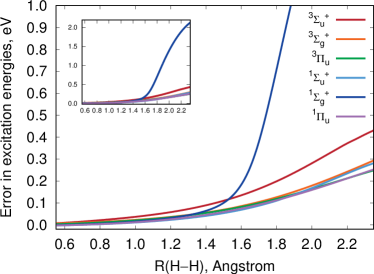
(a)

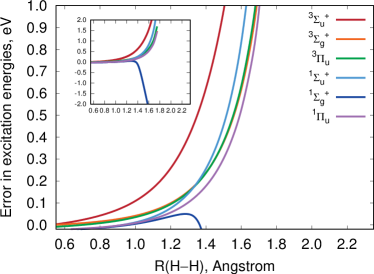
(b)

Figure 1: Errors in vertical excitation energies (eV) for six lowest-lying electronic states of H2 computed using LR-ODC-12 (1a) and LR-OLCCD (1b) as a function of the H–H bond length, relative to full configuration interaction. All methods employed the d-aug-cc-pvtz basis set. In each figure, the inset shows the same plot for a larger range of errors.

One of the desirable properties of an electronic structure method is exactness for two-electron systems. While the ODC-12 method is not exact for two-electron systems, it has been shown to provide a very good description of the ground-state H2 dissociation curve, with errors of $\sim$ 1 kcal mol^-1 with respect to full configuration interaction (FCI) near the dissociation limit.⁵⁴ Here, we investigate the performance of LR-ODC-12 for the excited states of H2. Figure 1a shows the errors in vertical excitation energies for six lowest-lying electronic states as a function of the H-H distance, relative to FCI. The FCI energies were computed using the EOM-CCSD method, which is exact for two-electron systems. At the equilibrium geometry ($r_{e}$ = 0.742 Å) the errors in excitation energies for all states do not exceed 0.02 eV. Between 0.6 and 1.45 Å ($r\approx 2r_{e}$), the LR-ODC-12 excitation energies remain in good agreement with FCI, with errors less than 0.1 eV for all states. In this range, the largest error is observed for the ${}^{3}\Sigma_{u}^{+}$ state. For $r$ $\geq$ 1.5 Å, the error in the ${}^{1}\Sigma_{g}^{+}$ excited state energy rapidly increases from 0.10 eV (at 1.5 Å) to 2.13 eV (at 2.35 Å), while for other states the errors increase much more slowly. Analysis of the FCI wavefunction for the ${}^{1}\Sigma_{g}^{+}$ state shows a significant contribution from the $(1\sigma_{g})^{2}\rightarrow(1\sigma_{u})^{2}$ double excitation already at $r$ $=$ 1.55 Å. This contribution becomes dominant for $r$ $\geq$ 1.75 Å. Thus, the large LR-ODC-12 errors observed for the ${}^{1}\Sigma_{g}^{+}$ state are likely due to the increasingly large double-excitation character of this electronic state at long H-H bond distances. The second largest error near the dissociation is observed for the ${}^{3}\Sigma_{u}^{+}$ state (0.43 eV). For other electronic states, smaller errors of $\sim$ 0.25 eV are observed near the dissociation.

The importance of the non-linear terms in the LR-ODC-12 equations can be investigated by comparing the LR-ODC-12 and LR-OLCCD results. Figure 1b shows the errors in the LR-OLCCD vertical excitation energies as a function of the H-H bond length. Although near the equilibrium geometry the performance of LR-OLCCD and LR-ODC-12 is similar, the LR-OLCCD errors increase much faster with increasing H-H distance compared to LR-ODC-12. At $r$ = 1.3 Å, the LR-OLCCD error for the ${}^{3}\Sigma_{u}^{+}$ state (0.4 eV) is almost six times larger than the corresponding error from LR-ODC-12 (0.07 eV). For $r$ $\geq$ 1.35 Å, the LR-OLCCD errors for all excitation energies show very steep increase in magnitude, ranging from 1.5 to 4.7 eV already at $r$ = 1.75 Å. We were unable to converge the LR-OLCCD equations for $r$ $\geq$ 1.80 Å. Overall, our results demonstrate that the non-linear terms in LR-ODC-12 significantly improve the description of the excited states at long H-H distances where the electron correlation effects are stronger.

4.3 Benchmark: Small Molecules

Table 2: Errors in vertical excitation energies (eV) for singlet states computed using LR-OLCCD, LR-ODC-12, and EOM-CCSD, relative to EOM-CCSDT (aug-cc-pVTZ basis set). All electrons were correlated in all computations. Also shown are mean absolute errors ($\Delta_{\mathrm{MAE}}$), standard deviations ($\Delta_{\mathrm{STD}}$), and maximum absolute errors ($\Delta_{\mathrm{MAX}}$) computed for each method.

		$\Delta$EOM-CCSD	$\Delta$LR-OLCCD	$\Delta$LR-ODC-12	EOM-CCSDT
N2	${}^{1}\Pi_{g}$	0.18	0.08	0.20	9.29
	${}^{1}\Sigma_{u}^{-}$	0.23	0.15	0.09	9.84
	${}^{1}\Delta_{u}$	0.26	0.14	0.10	10.26
CO	${}^{1}\Pi$	0.16	0.09	0.17	8.46
	${}^{1}\Sigma^{-}$	0.19	$-$0.10	$-$0.01	9.89
	${}^{1}\Delta$	0.19	$-$0.22	$-$0.05	10.03
HCN	${}^{1}\Sigma^{-}$	0.16	0.05	0.00	8.25
	${}^{1}\Delta$	0.17	0.04	0.01	8.61
	${}^{1}\Pi$	0.17	0.05	0.20	9.12
HNC	${}^{1}\Pi$	0.15	$-$0.01	0.10	8.13
	${}^{1}\Sigma^{+}$	0.24	0.05	0.12	8.46
	${}^{1}\Sigma^{-}$	0.15	$-$0.09	0.04	8.67
	${}^{1}\Delta$	0.15	$-$0.18	$-$0.03	8.84
C2H2	${}^{1}\Sigma_{u}^{-}$	0.12	0.06	0.02	7.11
	${}^{1}\Delta_{u}$	0.10	0.07	0.03	7.45
H2CO	${}^{1}\mathrm{A_{2}}$	0.10	$-$0.07	0.02	3.95
$\Delta_{\mathrm{MAE}}$		0.17	0.09	0.08
$\Delta_{\mathrm{STD}}$		0.05	0.11	0.08
$\Delta_{\mathrm{MAX}}$		0.26	0.22	0.20

Table 3: Errors in vertical excitation energies (eV) for triplet states computed using LR-OLCCD, LR-ODC-12, and EOM-CCSD, relative to EOM-CCSDT (aug-cc-pVTZ basis set). All electrons were correlated in all computations. Also shown are mean absolute errors ($\Delta_{\mathrm{MAE}}$), standard deviations ($\Delta_{\mathrm{STD}}$), and maximum absolute errors ($\Delta_{\mathrm{MAX}}$) computed for each method.

		$\Delta$EOM-CCSD	$\Delta$LR-OLCCD	$\Delta$LR-ODC-12	EOM-CCSDT
N2	${}^{3}\Sigma_{u}^{+}$	0.11	0.04	$-$0.02	7.63
	${}^{3}\Pi_{g}$	0.15	0.06	0.11	8.00
	${}^{3}\Delta_{u}$	0.17	0.08	0.03	8.82
	${}^{3}\Sigma_{u}^{-}$	0.28	0.03	0.01	9.63
	${}^{3}\Pi_{u}$	0.14	$-$0.01	0.10	11.18
CO	${}^{3}\Pi$	0.12	0.06	0.08	6.27
	${}^{3}\Sigma^{+}$	0.05	$-$0.03	$-$0.03	8.38
	${}^{3}\Delta$	0.11	$-$0.07	$-$0.03	9.21
	${}^{3}\Sigma^{-}$	0.19	$-$0.18	$-$0.06	9.72a
HCN	${}^{3}\Sigma^{+}$	0.05	$-$0.04	$-$0.10	6.40
	${}^{3}\Delta$	0.13	$-$0.02	$-$0.06	7.40
	${}^{3}\Pi$	0.10	0.08	0.06	8.01
	${}^{3}\Sigma^{-}$	0.16	$-$0.10	$-$0.05	8.15a
HNC	${}^{3}\Pi$	0.09	0.00	0.03	6.06
	${}^{3}\Sigma^{+}$	0.04	$-$0.09	$-$0.11	7.20
	${}^{3}\Delta$	0.10	$-$0.14	$-$0.11	8.02
	${}^{3}\Sigma^{+}$	0.22	$-$0.05	0.04	8.38
	${}^{3}\Sigma^{-}$	0.15	$-$0.02	0.11	8.56a
C2H2	${}^{3}\Sigma_{u}^{+}$	0.01	$-$0.02	$-$0.08	5.52
	${}^{3}\Delta_{u}$	0.08	$-$0.02	$-$0.05	6.41
	${}^{3}\Sigma_{u}^{-}$	0.10	$-$0.03	$-$0.05	7.10a
H2CO	${}^{3}\mathrm{A_{2}}$	0.04	$-$0.02	0.01	3.56
	${}^{3}\mathrm{A_{1}}$	0.02	$-$0.06	$-$0.14	6.06
$\Delta_{\mathrm{MAE}}$		0.11	0.05	0.06
$\Delta_{\mathrm{STD}}$		0.06	0.07	0.07
$\Delta_{\mathrm{MAX}}$		0.28	0.18	0.14

• For CO, HCN, HNC, and C2H2, the ${}^{3}\Sigma^{-}$ (${}^{3}\Sigma_{u}^{-}$) excitation energies were obtained from EOM-CC(2,3), which energies were shifted to reproduce the EOM-CCSDT energy for the ${}^{1}\Sigma^{-}$ (${}^{1}\Sigma_{u}^{-}$) state.

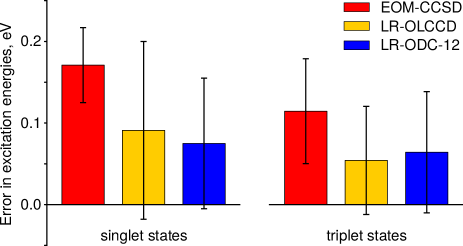
Figure 2: Mean absolute deviations ($\Delta_{\mathrm{MAE}}$) and standard deviations from the mean signed error ($\Delta_{\mathrm{STD}}$) for vertical excitation energies (Tables 2 and 3) computed using LR-OLCCD, LR-ODC-12, and EOM-CCSD, relative to EOM-CCSDT (aug-cc-pVTZ basis set). The $\Delta_{\mathrm{MAE}}$ value is represented as a height of each colored box, while the $\Delta_{\mathrm{STD}}$ value is depicted as a radius of the black vertical bar.

Here, we benchmark the performance of LR-ODC-12 for vertical excitation energies in several small molecules: N2, CO, HCN, HNC, C2H2, and H2CO. Tables 2 and 3 show the errors in excitation energies computed using EOM-CCSD, LR-OLCCD, and LR-ODC-12 for the singlet and triplet excited states, respectively, relative to the results from EOM-CCSDT. To measure the performance of each method, we computed the mean absolute errors ($\Delta_{\mathrm{MAE}}$) and the standard deviations from the average signed error ($\Delta_{\mathrm{STD}}$), shown in Figure 2.

For the singlet electronic states (Table 2), the excitation energies computed using LR-ODC-12 are in better agreement with EOM-CCSDT than those obtained from EOM-CCSD, on average. This is evidenced by $\Delta_{\mathrm{MAE}}$, which is smaller for LR-ODC-12 compared to EOM-CCSD by a factor of two ($\Delta_{\mathrm{MAE}}$ = 0.08 and 0.17 eV, respectively). The LR-ODC-12 errors exceed 0.10 eV for only four states, with a maximum error $\Delta_{\mathrm{MAX}}$ = 0.20 eV. EOM-CCSD has a minimum error of 0.10 eV, shows errors greater than 0.10 eV for 14 states, and has $\Delta_{\mathrm{MAX}}$ = 0.26 eV. EOM-CCSD shows a somewhat smaller $\Delta_{\mathrm{STD}}$ compared to that of LR-ODC-12 ($\Delta_{\mathrm{STD}}$ = 0.05 and 0.08 eV, respectively).

For the triplet states (Table 3), LR-ODC-12 is again superior to EOM-CCSD, on average, with $\Delta_{\mathrm{MAE}}$ = 0.06 and 0.11 eV for the two methods, respectively. LR-ODC-12 has errors larger than 0.10 eV for five states with $\Delta_{\mathrm{MAX}}$ = 0.14 eV, whereas EOM-CCSD exceeds 0.10 eV error for 12 states and shows $\Delta_{\mathrm{MAX}}$ = 0.28 eV. For linear molecules, EOM-CCSD exhibits consistently poor results for the ${}^{3}\Sigma^{-}$ electronic states, while the performance of LR-ODC-12 for different electronic states is similar. Notably, all EOM-CCSD excitation energies overestimate the EOM-CCSDT values, while the LR-ODC-12 energies are centered around the reference energies, suggesting that LR-ODC-12 provides a more balanced description of the ground and excited states.

Comparing LR-ODC-12 with LR-OLCCD, we see that both methods show very similar results for the triplet states ($\Delta_{\mathrm{MAE}}$ = 0.06 and 0.05 eV, respectively), with noticeable differences observed only for the ${}^{3}\Sigma^{-}$ states. For the singlet electronic states, LR-OLCCD shows a somewhat larger $\Delta_{\mathrm{MAE}}$ = 0.09 eV and $\Delta_{\mathrm{STD}}$ = 0.11 eV compared to LR-ODC-12 ($\Delta_{\mathrm{MAE}}$ = 0.08 eV and $\Delta_{\mathrm{STD}}$ = 0.08 eV). In this case, significant differences are observed for the ${}^{1}\Pi$ states of N2 and HCN, ${}^{1}\Sigma^{-}$ of HNC, and ${}^{1}\Delta$ of CO and HNC, indicating that the non-linear terms included in LR-ODC-12 are important for these electronic states.

4.4 Ethylene, Butadiene, and Hexatriene

Table 4: Ground-state total energies ($E_{\mathrm{h}}$) and vertical excitation energies (eV) computed using LR-OLCCD, LR-ODC-12, and EOM-CCSD for the low-lying electronic states of ethylene (C2H4), butadiene (C4H6), and hexatriene (C6H8). Computations employed the ANO-L-pVDZ (for C4H6 and C6H8) and ANO-L-pVTZ (for C2H4) basis sets and the MP2/cc-pVQZ optimized geometries. For LR-OLCCD and LR-ODC-12, oscillator strengths of the allowed transitions are given in parentheses. All electrons were correlated in all computations.

		EOM-CCSD	LR-OLCCD	LR-ODC-12	SHCIa
C2H4	$1{}^{1}\mathrm{A_{1g}}$	$-$78.441518	$-$78.455352	$-$78.450874	$-$78.4381
	$1{}^{3}\mathrm{B_{1u}}$	4.46	4.66	4.52	4.59
	$1{}^{1}\mathrm{B_{1u}}$	8.14	8.20 (1.8)	8.13 (1.9)	8.05
C4H6	$1{}^{1}\mathrm{A_{g}}$	$-$155.546920	$-$155.568356	$-$155.559882	$-$155.5582
	$1{}^{3}\mathrm{B_{u}}$	3.20	3.58	3.43	3.37
	$1{}^{1}\mathrm{B_{u}}$	6.53	6.76 (4.2)	6.67 (4.4)	6.45
	$2{}^{1}\mathrm{A_{g}}$	7.28	7.14	6.81	6.58
C6H8	$1{}^{1}\mathrm{A_{g}}$	$-$232.737880	$-$232.771738	$-$232.758675	$-$232.7567
	$1{}^{3}\mathrm{B_{u}}$	2.64	3.01	2.83	2.77
	$1{}^{1}\mathrm{B_{u}}$	5.60	5.89 (6.5)	5.74 (8.1)	5.59
	$2{}^{1}\mathrm{A_{g}}$	6.55	4.21	5.73	5.58

• Also shown are the energies from the semistochastic heat-bath CI (SHCI) method, extrapolated to the full CI limit.¹¹³ The $1s$ orbitals of carbon atoms were not included in the SHCI correlation treatment. The SHCI computations used the same basis sets and optimized geometries as those used for LR-OLCCD, LR-ODC-12, and EOM-CCSD.

Finally, we apply the LR-ODC-12 method to challenging excited states of ethylene (C2H4), butadiene (C4H6), and hexatriene (C6H8). A reliable description of these electronic states requires an accurate treatment of electron correlation. ^{114, 115, 116, 117, 118, 119, 120, 121, 122, 123, 124, 125, 126, 127, 111, 128, 112} All three molecules feature a dipole-allowed $1{}^{1}\mathrm{B_{u}}$ (or $1{}^{1}\mathrm{B_{1u}}$) state that is well described as a $\pi-\pi^{*}$ excitation, but requires a very accurate description of dynamic correlation between the $\sigma$ and $\pi$ electrons. In butadiene and hexatriene, the $1{}^{1}\mathrm{B_{u}}$ state is near-degenerate with a dipole-forbidden $2{}^{1}\mathrm{A_{g}}$ state that has a substantial double-excitation character, requiring the description of static correlation in the $\pi$ and $\pi^{*}$ orbitals.^{122, 123, 124} For this reason, the relative energies and ordering of the $1{}^{1}\mathrm{B_{u}}$ and $2{}^{1}\mathrm{A_{g}}$ states are very sensitive to various levels of theory. For example, single-reference methods truncated to single and double excitations describe the $1{}^{1}\mathrm{B_{u}}$ state more accurately than the $2{}^{1}\mathrm{A_{g}}$ state, while multi-reference methods are more reliable for the $2{}^{1}\mathrm{A_{g}}$ state, missing important dynamic correlation for the $1{}^{1}\mathrm{B_{u}}$ state. Very recently, Chien et al.¹¹³ reported accurate vertical excitation energies for the low-lying states of ethylene, butadiene, and hexatriene computed using semistochastic heat-bath configuration interaction (SHCI) extrapolated to the full CI limit. In this section, we will use the SHCI results to benchmark the accuracy of the LR-ODC-12 method.

Table 4 reports the ground-state total energies and vertical excitation energies of ethylene, butadiene, and hexatriene computed using the EOM-CCSD, LR-OLCCD, and LR-ODC-12 methods, along with the SHCI results from Ref. 113. We refer to the $\mathrm{B_{1u}}$ states of C2H4 as $\mathrm{B_{u}}$ for brevity. All methods employed the same optimized geometries and basis sets (see Table 4 for details). We note that in the SHCI computations the $1s$ orbitals of carbon atoms were not included in the correlation treatment, while in other methods all electrons were correlated. To estimate the effect of the frozen-core approximation on the SHCI vertical excitation energies, we compared the excitation energies computed using the all-electron and frozen-core EOM-CCSD methods. The errors due to the frozen core did not exceed 0.01 eV.

All excitation energies decrease as the number of double bonds in a molecule increases. For butadiene and hexatriene, the ($1{}^{1}\mathrm{B_{u}}$; $2{}^{1}\mathrm{A_{g}}$) excitation energies computed using the SHCI method are (6.45; 6.58) and (5.59; 5.58) eV, respectively, indicating that the two states are nearly degenerate for the longer polyene. This feature is not reproduced by the EOM-CCSD method, which predicts the $1{}^{1}\mathrm{B_{u}}$ state energies in close agreement with SHCI, but significantly overestimates the energies for the doubly-excited $2{}^{1}\mathrm{A_{g}}$ state. As a result, the EOM-CCSD method overestimates the energy spacing between the $1{}^{1}\mathrm{B_{u}}$ and $2{}^{1}\mathrm{A_{g}}$ states by $\sim$ 0.6 eV and 1.0 eV for butadiene and hexatriene, respectively.

The LR-ODC-12 method, by contrast, correctly describes the relative energies and ordering of the $1{}^{1}\mathrm{B_{u}}$ and $2{}^{1}\mathrm{A_{g}}$ states. The energy spacing between these states computed using LR-ODC-12 is 0.14 and $-$0.01 eV for butadiene and hexatriene, respectively, in an excellent agreement with the SHCI results (0.13 and $-$0.01 eV). For the singlet excited states, the LR-ODC-12 method consistently overestimates the excitation energies by $\sim$ 0.1 – 0.2 eV, relative to SHCI. For the $1{}^{3}\mathrm{B_{u}}$ state, the LR-ODC-12 errors are smaller in magnitude ($\sim$ 0.06 eV). Importantly, these results suggest that the LR-ODC-12 method provides a balanced description of the excited states with different electronic structure effects, as illustrated by its consistent performance for the $1{}^{3}\mathrm{B_{u}}$, $1{}^{1}\mathrm{B_{u}}$, and $2{}^{1}\mathrm{A_{g}}$ states in ethylene, butadiene, and hexatriene.

Comparing to LR-OLCCD shows that including the non-linear terms in LR-ODC-12 is crucial for the description of excited states with double-excitation character. While for the $1{}^{3}\mathrm{B_{u}}$ and $1{}^{1}\mathrm{B_{u}}$ states the LR-OLCCD errors exceed the LR-ODC-12 errors by $\sim$ 0.15 eV, for the doubly-excited $2{}^{1}\mathrm{A_{g}}$ state the LR-OLCCD errors are much bigger: 0.56 and $-$1.37 eV for butadiene and hexatriene, respectively.

5 Conclusions

We have presented a new approach for excited electronic states based on the linear-response formulation of density cumulant theory (DCT). The resulting linear-response DCT model (LR-DCT) has the same computational scaling as the original (single-state) DCT formulation but can accurately predict energies and properties for many electronic states, simultaneously. We have described the general formulation of LR-DCT, derived equations for the linear-response ODC-12 method (LR-ODC-12), and presented its implementation. In LR-ODC-12, excited-state energies are obtained by solving the generalized eigenvalue equation that involves a symmetric Hessian matrix. This simplifies the computation of the excited-state properties (such as transition dipoles) and ensures that the excitation energies have real values, provided that the Hessian is positive semi-definite. In addition, the LR-ODC-12 excitation energies are size-intensive, which we have verified numerically for a system of noninteracting fragments.

Our preliminary results demonstrate that LR-ODC-12 yields very accurate excitation energies for a variety of excited states with different electronic structure effects. For a set of small molecules (N2, CO, HCN, HNC, C2H2, and H2CO), LR-ODC-12 outperforms equation-of-motion coupled cluster theory with single and double excitations (EOM-CCSD), with mean absolute errors in excitation energies of less than 0.1 eV, relative to reference data. Importantly, both LR-ODC-12 and EOM-CCSD have the same computational scaling. In a study of ethylene, butadiene, and hexatriene, we have compared the performance of LR-ODC-12 and EOM-CCSD with the results from highly-accurate semistochastic heat-bath configuration interaction (SHCI). For butadiene and hexatriene, LR-ODC-12 provides a balanced description of the singly-excited $1{}^{1}\mathrm{B_{u}}$ and the doubly-excited $2{}^{1}\mathrm{A_{g}}$ states, predicting that the two states become nearly-degenerate in hexatriene, in excellent agreement with SHCI. By contrast, EOM-CCSD drastically overestimates the energy of the $2{}^{1}\mathrm{A_{g}}$ state, resulting in a $\sim$ 1 eV error in the energy gap between these states of hexatriene.

Overall, our results demonstrate that linear-response density cumulant theory is a promising theoretical approach for spectroscopic properties of molecules and encourage its further development. Several research directions are worth exploring. One of them is the efficient implementation of LR-ODC-12 and its applications to chemical systems with challenging electronic states. Two classes of systems that are particularly worth exploring are open-shell molecules and transition metal complexes. Another direction is to extend LR-DCT to simulations of other spectroscopic properties, such as photoelectron or X-ray absorption spectra. In this regard, applying LR-DCT to the computation of optical rotation properties is of particular interest as it is expected to avoid gauge invariance problems due to the variational nature of the DCT orbitals.¹²⁹ We plan to explore these directions in the future.

Appendix A Derivatives of the One-Body Density Matrix in Density Cumulant Theory

Repeated differentiation of the one-body $n$-representability condition (Eq. 3) gives the following formulas for the first and second derivatives of the cumulant partial trace:

$$\begin{array}[]{r@{\,}l}\dfrac{\partial\lambda^{pr}_{qr}}{\partial{y}}=\gamma^{p}_{s}\dfrac{\partial\gamma^{s}_{q}}{\partial{y}}+\dfrac{\partial\gamma^{p}_{s}}{\partial{y}}\gamma^{s}_{q}-\dfrac{\partial\gamma^{p}_{q}}{\partial{y}}\end{array}$$ (35)

$$\begin{array}[]{r@{\,}l}\dfrac{\partial^{2}\lambda^{pr}_{qr}}{\partial{x}\partial{y}}=&\gamma^{p}_{s}\dfrac{\partial\gamma^{s}_{q}}{\partial{x}\partial{y}}+\dfrac{\partial\gamma^{p}_{s}}{\partial{x}\partial{y}}\gamma^{s}_{q}-\dfrac{\partial\gamma^{p}_{q}}{\partial{x}\partial{y}}\\[15.0pt] &+\dfrac{\partial\gamma^{p}_{s}}{\partial{x}}\dfrac{\partial\gamma^{s}_{q}}{\partial{y}}+\dfrac{\partial\gamma^{s}_{q}}{\partial{x}}\dfrac{\partial\gamma^{p}_{s}}{\partial{y}}\end{array}$$ (36)

Transforming to the natural spin-orbital basis (NSO, denoted by prime indices) where the one-body density matrix is diagonal, the first and second derivatives of the one-body density matrix can be determined from the cumulant derivatives as follows:

$$\begin{array}[]{r@{\,}l}\dfrac{\partial\gamma^{p^{\prime}}_{q^{\prime}}}{\partial{y}}=&\theta_{p^{\prime}q^{\prime}}\dfrac{\partial\lambda^{p^{\prime}r}_{q^{\prime}r}}{\partial{y}}\end{array}$$ (37)

$$\begin{array}[]{r@{\,}l}\dfrac{\partial^{2}\gamma^{p^{\prime}}_{q^{\prime}}}{\partial{x}\partial{y}}=&\theta_{p^{\prime}q^{\prime}}\dfrac{\partial^{2}\lambda^{p^{\prime}r}_{q^{\prime}r}}{\partial{x}\partial{y}}-\delta_{r^{\prime}}^{s^{\prime}}\theta_{p^{\prime}q^{\prime}}\theta_{p^{\prime}s^{\prime}}\theta_{q^{\prime}r^{\prime}}\dfrac{\partial\lambda^{p^{\prime}t}_{s^{\prime}t}}{\partial{x}}\dfrac{\partial\lambda^{r^{\prime}u}_{q^{\prime}u}}{\partial{y}}\\[15.0pt] &-\delta_{r^{\prime}}^{s^{\prime}}\theta_{p^{\prime}q^{\prime}}\theta_{p^{\prime}s^{\prime}}\theta_{q^{\prime}r^{\prime}}\dfrac{\partial\lambda^{r^{\prime}u}_{q^{\prime}u}}{\partial{x}}\dfrac{\partial\lambda^{p^{\prime}t}_{s^{\prime}t}}{\partial{y}}\end{array}$$ (38)

Here, we have defined the following matrix:

$$\theta_{p^{\prime}q^{\prime}}\equiv\left\{\begin{array}[]{cc}(\gamma_{p^{\prime}}+\gamma_{q^{\prime}}-1)^{-1}&\text{if $p^{\prime},q^{\prime}\in\mathrm{occ\ or\ vir}$ }\\ 0&\text{otherwise}\end{array}\right.$$ (39)

where $\gamma_{p^{\prime}}$ denotes an eigenvalue of the one-body density matrix (i.e., an occupation number). The natural spin-orbital $p^{\prime}$ is considered occupied if $\gamma_{p^{\prime}}>0.5$.

Eqs. 37 and 38 can be used to derive expressions for the two-body energy Hessian in Eq. 26. Simplifying the resulting equations allows us to determine the intermediates defined in Eq. 27. In the NSO basis, these intermediates are given by

$$\mathcal{F}_{p^{\prime}}^{q^{\prime}}\equiv\theta_{p^{\prime}q^{\prime}}f_{p^{\prime}}^{q^{\prime}}$$ (40)

$$\mathcal{G}_{p^{\prime}r^{\prime}}^{q^{\prime}s^{\prime}}\equiv\theta_{p^{\prime}q^{\prime}}\theta_{r^{\prime}s^{\prime}}(\overline{g}_{p^{\prime}r^{\prime}}^{q^{\prime}s^{\prime}}-\mathcal{F}_{p^{\prime}}^{s^{\prime}}\delta_{r^{\prime}}^{q^{\prime}}-\mathcal{F}_{r^{\prime}}^{q^{\prime}}\delta_{p^{\prime}}^{s^{\prime}})$$ (41)

These quantities are computed in the NSO basis and back-transformed to the original spin-orbital basis using the eigenvectors of the one-particle density matrix (see Ref. 53 for more details).

A.V.C. was supported by NSF grant CHE-1661604. A.Y.S. was supported by start-up funds provided by the Ohio State University.

Formulas for the energy Hessian ($\mathbf{E}$), the metric matrix ($\mathbf{M}$), and the property gradient vector ($\mathbf{v}^{\prime}$) for the LR-ODC-12 and LR-OLCCD methods are included in the Supporting Information.

References

- Knowles and Werner 1985 Knowles, P. J.; Werner, H.-J. An efficient second-order MC SCF method for long configuration expansions. Chem. Phys. Lett. 1985, 115, 259–267
- Wolinski et al. 1987 Wolinski, K.; Sellers, H. L.; Pulay, P. Consistent generalization of the Møller-Plesset partitioning to open-shell and multiconfigurational SCF reference states in many-body perturbation theory. Chem. Phys. Lett. 1987, 140, 225–231
- Hirao 1992 Hirao, K. Multireference Møller—Plesset method. Chem. Phys. Lett. 1992, 190, 374–380
- Finley et al. 1998 Finley, J.; Malmqvist, P. Å.; Roos, B. O.; Serrano-Andrés, L. The multi-state CASPT2 method. Chem. Phys. Lett. 1998, 288, 299–306
- Andersson et al. 1990 Andersson, K.; Malmqvist, P. Å.; Roos, B. O.; Sadlej, A. J.; Wolinski, K. Second-order perturbation theory with a CASSCF reference function. J. Phys. Chem. 1990, 94, 5483–5488
- Andersson et al. 1992 Andersson, K.; Malmqvist, P. Å.; Roos, B. O. Second-order perturbation theory with a complete active space self-consistent field reference function. J. Chem. Phys. 1992, 96, 1218–1226
- Angeli et al. 2001 Angeli, C.; Cimiraglia, R.; Evangelisti, S.; Leininger, T.; Malrieu, J.-P. P. Introduction of n-electron valence states for multireference perturbation theory. J. Chem. Phys. 2001, 114, 10252–10264
- Angeli et al. 2001 Angeli, C.; Cimiraglia, R.; Malrieu, J.-P. P. N-electron valence state perturbation theory: a fast implementation of the strongly contracted variant. Chem. Phys. Lett. 2001, 350, 297–305
- Mukherjee et al. 1977 Mukherjee, D.; Moitra, R. K.; Mukhopadhyay, A. Applications of a non-perturbative many-body formalism to general open-shell atomic and molecular problems: calculation of the ground and the lowest -* singlet and triplet energies and the first ionization potential of trans-butadiene. Mol. Phys. 1977, 33, 955–969
- Jeziorski and Monkhorst 1981 Jeziorski, B.; Monkhorst, H. J. Coupled-cluster method for multideterminantal reference states. Phys. Rev. A 1981, 24, 1668–1681
- Werner and Knowles 1988 Werner, H.-J.; Knowles, P. J. An efficient internally contracted multiconfiguration–reference configuration interaction method. J. Chem. Phys. 1988, 89, 5803–5814
- Mahapatra et al. 1998 Mahapatra, U. S.; Datta, B.; Mukherjee, D. A state-specific multi-reference coupled cluster formalism with molecular applications. Mol. Phys. 1998, 94, 157–171
- Pittner 2003 Pittner, J. Continuous transition between Brillouin–Wigner and Rayleigh–Schrödinger perturbation theory, generalized Bloch equation, and Hilbert space multireference coupled cluster. J. Chem. Phys. 2003, 118, 10876
- Evangelista et al. 2007 Evangelista, F. A.; Allen, W. D.; Schaefer, H. F. Coupling term derivation and general implementation of state-specific multireference coupled cluster theories. J. Chem. Phys. 2007, 127, 024102
- Datta et al. 2011 Datta, D.; Kong, L.; Nooijen, M. A state-specific partially internally contracted multireference coupled cluster approach. J. Chem. Phys. 2011, 134, 214116–214116–19
- Evangelista and Gauss 2011 Evangelista, F. A.; Gauss, J. An orbital-invariant internally contracted multireference coupled cluster approach. J. Chem. Phys. 2011, 134, 114102
- Köhn et al. 2013 Köhn, A.; Hanauer, M.; Mück, L. A.; Jagau, T.-C.; Gauss, J. State-specific multireference coupled-cluster theory. WIREs Comput. Mol. Sci. 2013, 3, 176–197
- Nooijen et al. 2014 Nooijen, M.; Demel, O.; Datta, D.; Kong, L.; Shamasundar, K. R.; Lotrich, V.; Huntington, L. M.; Neese, F. Communication: Multireference equation of motion coupled cluster: A transform and diagonalize approach to electronic structure. J. Chem. Phys. 2014, 140, 081102
- Foresman et al. 1992 Foresman, J. B.; Head-Gordon, M.; Pople, J. A.; Frisch, M. J. Toward a systematic molecular orbital theory for excited states. J. Phys. Chem. 1992, 96, 135–149
- Sherrill and Schaefer 1999 Sherrill, C. D.; Schaefer, H. F. The Configuration Interaction Method: Advances in Highly Correlated Approaches. Adv. Quant. Chem. 1999, 34, 143–269
- Geertsen et al. 1989 Geertsen, J.; Rittby, M.; Bartlett, R. J. The equation-of-motion coupled-cluster method: Excitation energies of Be and CO. Chem. Phys. Lett. 1989, 164, 57–62
- Comeau and Bartlett 1993 Comeau, D. C.; Bartlett, R. J. The equation-of-motion coupled-cluster method. Applications to open- and closed-shell reference states. Chem. Phys. Lett. 1993, 207, 414–423
- Stanton and Bartlett 1993 Stanton, J. F.; Bartlett, R. J. The equation of motion coupled-cluster method. A systematic biorthogonal approach to molecular excitation energies, transition probabilities, and excited state properties. J. Chem. Phys. 1993, 98, 7029
- Krylov 2008 Krylov, A. I. Equation-of-Motion Coupled-Cluster Methods for Open-Shell and Electronically Excited Species: The Hitchhiker’s Guide to Fock Space. Annu. Rev. Phys. Chem. 2008, 59, 433–462
- Crawford and Schaefer 2000 Crawford, T. D.; Schaefer, H. F. An Introduction to Coupled Cluster Theory for Computational Chemists. Rev. Comp. Chem. 2000, 14, 33–136
- Shavitt and Bartlett 2009 Shavitt, I.; Bartlett, R. J. Many-Body Methods in Chemistry and Physics; Cambridge University Press: Cambridge, UK, 2009
- Sekino and Bartlett 1984 Sekino, H.; Bartlett, R. J. A linear response, coupled-cluster theory for excitation energy. Int. J. Quantum Chem. 1984, 26, 255–265
- Koch et al. 1990 Koch, H.; Jensen, H. J. A.; Jørgensen, P.; Helgaker, T. Excitation energies from the coupled cluster singles and doubles linear response function (CCSDLR). Applications to Be, CH+, CO, and H2O. J. Chem. Phys. 1990, 93, 3345–3350
- Koch and Jørgensen 1990 Koch, H.; Jørgensen, P. Coupled cluster response functions. J. Chem. Phys. 1990, 93, 3333–3344
- Nooijen and Bartlett 1997 Nooijen, M.; Bartlett, R. J. A new method for excited states: Similarity transformed equation-of-motion coupled-cluster theory. J. Chem. Phys. 1997, 106, 6441–6448
- Nooijen and Bartlett 1997 Nooijen, M.; Bartlett, R. J. Similarity transformed equation-of-motion coupled-cluster theory: Details, examples, and comparisons. J. Chem. Phys. 1997, 107, 6812–6830
- Nakatsuji and Hirao 1978 Nakatsuji, H.; Hirao, K. Cluster expansion of the wavefunction. Symmetry-adapted-cluster expansion, its variational determination, and extension of open-shell orbital theory. J. Chem. Phys. 1978, 68, 2053–2065
- Nakatsuji 1979 Nakatsuji, H. Cluster expansion of the wavefunction. Electron correlations in ground and excited states by SAC (symmetry-adapted-cluster) and SAC CI theories. Chem. Phys. Lett. 1979, 67, 329–333
- Stanton 1993 Stanton, J. F. Many-body methods for excited state potential energy surfaces. I. General theory of energy gradients for the equation-of-motion coupled-cluster method. J. Chem. Phys. 1993, 99, 8840–8847
- Stanton and Gauss 1994 Stanton, J. F.; Gauss, J. Analytic energy gradients for the equation-of-motion coupled-cluster method: Implementation and application to the HCN/HNC system. J. Chem. Phys. 1994, 100, 4695–4698
- Stanton and Gauss 1994 Stanton, J. F.; Gauss, J. Analytic energy derivatives for ionized states described by the equation-of-motion coupled cluster method. J. Chem. Phys. 1994, 101, 8938–8944
- Levchenko et al. 2005 Levchenko, S. V.; Wang, T.; Krylov, A. I. Analytic gradients for the spin-conserving and spin-flipping equation-of-motion coupled-cluster models with single and double substitutions. J. Chem. Phys. 2005, 122, 224106
- Hättig 2005 Hättig, C. Structure Optimizations for Excited States with Correlated Second-Order Methods: CC2 and ADC(2). Adv. Quant. Chem. 2005, 50, 37 – 60
- Köhn and Tajti 2007 Köhn, A.; Tajti, A. Can coupled-cluster theory treat conical intersections? J. Chem. Phys. 2007, 127, 044105
- Kjønstad et al. 2017 Kjønstad, E. F.; Myhre, R. H.; Martínez, T. J.; Koch, H. Crossing conditions in coupled cluster theory. J. Chem. Phys. 2017, 147, 164105
- Schirmer 1982 Schirmer, J. Beyond the random-phase approximation: A new approximation scheme for the polarization propagator. Phys. Rev. A 1982, 26, 2395–2416
- Schirmer 1991 Schirmer, J. Closed-form intermediate representations of many-body propagators and resolvent matrices. Phys. Rev. A 1991, 43, 4647
- Dreuw and Wormit 2014 Dreuw, A.; Wormit, M. The algebraic diagrammatic construction scheme for the polarization propagator for the calculation of excited states. WIREs Comput. Mol. Sci. 2014, 5, 82–95
- Taube and Bartlett 2006 Taube, A. G.; Bartlett, R. J. New perspectives on unitary coupled-cluster theory. Int. J. Quantum Chem. 2006, 106, 3393–3401
- Kats et al. 2011 Kats, D.; Usvyat, D.; Schütz, M. Second-order variational coupled-cluster linear-response method: A Hermitian time-dependent theory. Phys. Rev. A 2011, 83, 062503
- Wälz et al. 2012 Wälz, G.; Kats, D.; Usvyat, D.; Korona, T.; Schütz, M. Application of Hermitian time-dependent coupled-cluster response Ansätze of second order to excitation energies and frequency-dependent dipole polarizabilities. Phys. Rev. A 2012, 86, 052519
- Kjønstad and Koch 2017 Kjønstad, E. F.; Koch, H. Resolving the Notorious Case of Conical Intersections for Coupled Cluster Dynamics. J. Phys. Chem. Lett. 2017, 8, 4801–4807
- Moszynski et al. 2005 Moszynski, R.; Żuchowski, P. S.; Jeziorski, B. Time-Independent Coupled-Cluster Theory of the Polarization Propagator. Collect. Czech. Chem. Commun. 2005, 70, 1109–1132
- Korona 2010 Korona, T. XCC2—a new coupled cluster model for the second-order polarization propagator. Phys. Chem. Chem. Phys. 2010, 12, 14977–14984
- Kutzelnigg 2006 Kutzelnigg, W. Density-cumulant functional theory. J. Chem. Phys. 2006, 125, 171101
- Simmonett et al. 2010 Simmonett, A. C.; Wilke, J. J.; Schaefer, H. F.; Kutzelnigg, W. Density cumulant functional theory: First implementation and benchmark results for the DCFT-06 model. J. Chem. Phys. 2010, 133, 174122
- Sokolov et al. 2012 Sokolov, A. Y.; Wilke, J. J.; Simmonett, A. C.; Schaefer, H. F. Analytic gradients for density cumulant functional theory: The DCFT-06 model. J. Chem. Phys. 2012, 137, 054105–054105–7
- Sokolov et al. 2013 Sokolov, A. Y.; Simmonett, A. C.; Schaefer, H. F. Density cumulant functional theory: The DC-12 method, an improved description of the one-particle density matrix. J. Chem. Phys. 2013, 138, 024107–024107–9
- Sokolov and Schaefer 2013 Sokolov, A. Y.; Schaefer, H. F. Orbital-optimized density cumulant functional theory. J. Chem. Phys. 2013, 139, 204110–204110
- Sokolov et al. 2014 Sokolov, A. Y.; Schaefer, H. F.; Kutzelnigg, W. Density cumulant functional theory from a unitary transformation: N-representability, three-particle correlation effects, and application to O4+. J. Chem. Phys. 2014, 141, 074111
- Wang et al. 2016 Wang, X.; Sokolov, A. Y.; Turney, J. M.; Schaefer, H. F. Spin-Adapted Formulation and Implementation of Density Cumulant Functional Theory with Density-Fitting Approximation: Application to Transition Metal Compounds. J. Chem. Theory Comput. 2016, 12, 4833–4842
- 57 We note that early on DCT was referred to as “density cumulant functional theory” (DCFT).
- Fulde 1991 Fulde, P. Electron Correlations in Molecules and Solids; Springer: Berlin, 1991
- Ziesche 1992 Ziesche, P. Definition of exchange based on cumulant expansion: Correlation induced narrowing of the exchange hole. Solid State Commun 1992, 82, 597–602
- Kutzelnigg and Mukherjee 1997 Kutzelnigg, W.; Mukherjee, D. Normal order and extended Wick theorem for a multiconfiguration reference wave function. J. Chem. Phys. 1997, 107, 432
- Mazziotti 1998 Mazziotti, D. A. Approximate solution for electron correlation through the use of Schwinger probes. Chem. Phys. Lett. 1998, 289, 419–427
- Mazziotti 1998 Mazziotti, D. A. Contracted Schrödinger equation: Determining quantum energies and two-particle density matrices without wave functions. Phys. Rev. A 1998, 57, 4219–4234
- Kutzelnigg and Mukherjee 1999 Kutzelnigg, W.; Mukherjee, D. Cumulant expansion of the reduced density matrices. J. Chem. Phys. 1999, 110, 2800–2809
- Ziesche 2000 Ziesche, P. In Many-Electron Densities and Reduced Density Matrices; Cioslowski, J., Ed.; Springer US: Boston, MA, 2000; pp 33–56
- Herbert and Harriman 2007 Herbert, J. M.; Harriman, J. E. Cumulants, Extensivity, and the Connected Formulation of the Contracted Schrödinger Equation. Adv. Chem. Phys. 2007, 134, 261
- Kong and Valeev 2011 Kong, L.; Valeev, E. F. A novel interpretation of reduced density matrix and cumulant for electronic structure theories. J. Chem. Phys. 2011, 134, 214109–214109–9
- Hanauer and Köhn 2012 Hanauer, M.; Köhn, A. Meaning and magnitude of the reduced density matrix cumulants. Chem. Phys. 2012, 401, 50–61
- Colmenero and Valdemoro 1993 Colmenero, F.; Valdemoro, C. Approximating q-order reduced density matrices in terms of the lower-order ones. II. Applications. Phys. Rev. A 1993, 47, 979–985
- Nakatsuji and Yasuda 1996 Nakatsuji, H.; Yasuda, K. Direct Determination of the Quantum-Mechanical Density Matrix Using the Density Equation. Phys. Rev. Lett. 1996, 76, 1039–1042
- Nakata et al. 2001 Nakata, M.; Nakatsuji, H.; Ehara, M.; Fukuda, M.; Nakata, K.; Fujisawa, K. Variational calculations of fermion second-order reduced density matrices by semidefinite programming algorithm. J. Chem. Phys. 2001, 114, 8282
- Nakata et al. 2002 Nakata, M.; Ehara, M.; Nakatsuji, H. Density matrix variational theory: Application to the potential energy surfaces and strongly correlated systems. J. Chem. Phys. 2002, 116, 5432–5439
- Mazziotti 2006 Mazziotti, D. A. Anti-Hermitian Contracted Schrödinger Equation: Direct Determination of the Two-Electron Reduced Density Matrices of Many-Electron Molecules. Phys. Rev. Lett. 2006, 97, 143002
- Kollmar 2006 Kollmar, C. A size extensive energy functional derived from a double configuration interaction approach: The role of N representability conditions. J. Chem. Phys. 2006, 125, 084108
- DePrince and Mazziotti 2007 DePrince, A. E.; Mazziotti, D. A. Parametric approach to variational two-electron reduced-density-matrix theory. Phys. Rev. A 2007, 76, 042501
- DePrince 2016 DePrince, A. E. Variational optimization of the two-electron reduced-density matrix under pure-state N-representability conditions. J. Chem. Phys. 2016, 145, 164109
- Mazziotti 2008 Mazziotti, D. A. Parametrization of the Two-Electron Reduced Density Matrix for its Direct Calculation without the Many-Electron Wave Function. Phys. Rev. Lett. 2008, 101, 253002
- Mazziotti 2010 Mazziotti, D. A. Parametrization of the two-electron reduced density matrix for its direct calculation without the many-electron wave function: Generalizations and applications. Phys. Rev. A 2010, 81, 062515
- DePrince and Mazziotti 2012 DePrince, A. E.; Mazziotti, D. A. Connection of an elementary class of parametric two-electron reduced-density-matrix methods to the coupled electron-pair approximations. Mol. Phys. 2012, 110, 1917–1925
- Kutzelnigg 1991 Kutzelnigg, W. Error analysis and improvements of coupled-cluster theory. Theor. Chem. Acc. 1991, 80, 349–386
- Kutzelnigg 1998 Kutzelnigg, W. Almost variational coupled cluster theory. Mol. Phys. 1998, 94, 65–71
- Van Voorhis and Head-Gordon 2000 Van Voorhis, T.; Head-Gordon, M. Benchmark variational coupled cluster doubles results. J. Chem. Phys. 2000, 113, 8873
- Kutzelnigg 1982 Kutzelnigg, W. Quantum chemistry in Fock space. I. The universal wave and energy operators. J. Chem. Phys. 1982, 77, 3081–3097
- Bartlett et al. 1989 Bartlett, R. J.; Kucharski, S. A.; Noga, J. Alternative coupled-cluster ansätze II. The unitary coupled-cluster method. Chem. Phys. Lett. 1989, 155, 133–140
- Watts et al. 1989 Watts, J. D.; Trucks, G. W.; Bartlett, R. J. The unitary coupled-cluster approach and molecular properties. Applications of the UCC(4) method. Chem. Phys. Lett. 1989, 157, 359–366
- Szalay et al. 1995 Szalay, P. G.; Nooijen, M.; Bartlett, R. J. Alternative ansätze in single reference coupled-cluster theory. III. A critical analysis of different methods. J. Chem. Phys. 1995, 103, 281–298
- Cooper and Knowles 2010 Cooper, B.; Knowles, P. J. Benchmark studies of variational, unitary and extended coupled cluster methods. J. Chem. Phys. 2010, 133, 234102
- Evangelista 2011 Evangelista, F. A. Alternative single-reference coupled cluster approaches for multireference problems: The simpler, the better. J. Chem. Phys. 2011, 134, 224102–224102–13
- Nakata and Yasuda 2009 Nakata, M.; Yasuda, K. Size extensivity of the variational reduced-density-matrix method. Phys. Rev. A 2009, 80, 042109
- Van Aggelen et al. 2010 Van Aggelen, H.; Verstichel, B.; Bultinck, P.; Van Neck, D.; Ayers, P. W.; Cooper, D. L. Chemical verification of variational second-order density matrix based potential energy surfaces for the N[sub 2] isoelectronic series. J. Chem. Phys. 2010, 132, 114112
- Verstichel et al. 2010 Verstichel, B.; Van Aggelen, H.; Van Neck, D.; Ayers, P. W.; Bultinck, P. Subsystem constraints in variational second order density matrix optimization: Curing the dissociative behavior. J. Chem. Phys. 2010, 132, 114113
- Scheiner et al. 1987 Scheiner, A. C.; Scuseria, G. E.; Rice, J. E.; Lee, T. J.; Schaefer, H. F. Analytic evaluation of energy gradients for the single and double excitation coupled cluster (CCSD) wave function: Theory and application. J. Chem. Phys. 1987, 87, 5361–5373
- Salter et al. 1989 Salter, E. A.; Trucks, G. W.; Bartlett, R. J. Analytic energy derivatives in many-body methods. I. First derivatives. J. Chem. Phys. 1989, 90, 1752–1766
- Gauss et al. 1991 Gauss, J.; Stanton, J. F.; Bartlett, R. J. Coupled-cluster open-shell analytic gradients: Implementation of the direct product decomposition approach in energy gradient calculations. J. Chem. Phys. 1991, 95, 2623
- Gauss et al. 1991 Gauss, J.; Lauderdale, W. J.; Stanton, J. F.; Watts, J. D.; Bartlett, R. J. Analytic energy gradients for open-shell coupled-cluster singles and doubles (CCSD) calculations using restricted open-shell Hartree—Fock (ROHF) reference functions. Chem. Phys. Lett. 1991, 182, 207–215
- Copan et al. 2014 Copan, A. V.; Sokolov, A. Y.; Schaefer, H. F. Benchmark Study of Density Cumulant Functional Theory: Thermochemistry and Kinetics. J. Chem. Theory Comput. 2014, 10, 2389–2398
- Mullinax et al. 2015 Mullinax, J. W.; Sokolov, A. Y.; Schaefer, H. F. Can Density Cumulant Functional Theory Describe Static Correlation Effects? J. Chem. Theory Comput. 2015, 11, 2487–2495
- Bozkaya and Sherrill 2013 Bozkaya, U.; Sherrill, C. D. Orbital-optimized coupled-electron pair theory and its analytic gradients: Accurate equilibrium geometries, harmonic vibrational frequencies, and hydrogen transfer reactions. J. Chem. Phys. 2013, 139, 054104–054104–12
- Norman 2011 Norman, P. A Perspective on Nonresonant and Resonant Electronic Response Theory for Time-Dependent Molecular Properties. Phys. Chem. Chem. Phys. 2011, 13, 20519–20535
- Helgaker et al. 2012 Helgaker, T.; Coriani, S.; Jørgensen, P.; Kristensen, K.; Olsen, J.; Ruud, K. Recent Advances in Wave Function-Based Methods of Molecular-Property Calculations. Chem. Rev. 2012, 112, 543–631
- Kristensen et al. 2009 Kristensen, K.; Kauczor, J.; Kjærgaard, T.; Jørgensen, P. Quasienergy Formulation of Damped Response Theory. J. Chem. Phys. 2009, 131, 044112
- Olsen and Jørgensen 1985 Olsen, J.; Jørgensen, P. Linear and Nonlinear Response Functions for an Exact State and for an MCSCF State. J. Chem. Phys. 1985, 82, 3235–3264
- Sauer 2011 Sauer, S. P. A. Molecular Electromagnetism: A Computational Chemistry Approach; Oxford University Press: Oxford, 2011
- Parrish et al. 2017 Parrish, R. M.; Burns, L. A.; Smith, D. G. A.; Simmonett, A. C.; DePrince, A. E.; Hohenstein, E. G.; Bozkaya, U.; Sokolov, A. Y.; Di Remigio, R.; Richard, R. M.; Gonthier, J. F.; James, A. M.; McAlexander, H. R.; Kumar, A.; Saitow, M.; Wang, X.; Pritchard, B. P.; Verma, P.; Schaefer, H. F.; Patkowski, K.; King, R. A.; Valeev, E. F.; Evangelista, F. A.; Turney, J. M.; Crawford, T. D.; Sherrill, C. D. Psi41.1: An Open-Source Electronic Structure Program Emphasizing Automation, Advanced Libraries, and Interoperability. J. Chem. Theory Comput. 2017, 13, 3185–3197
- Sun et al. 2018 Sun, Q.; Berkelbach, T. C.; Blunt, N. S.; Booth, G. H.; Guo, S.; Li, Z.; Liu, J.; McClain, J. D.; Sayfutyarova, E. R.; Sharma, S.; Wouters, S.; Chan, G. K.-L. PySCF: the Python-based simulations of chemistry framework. WIREs Comput. Mol. Sci. 2018, 8, e1340
- Davidson 1975 Davidson, E. R. The Iterative Calculation of a Few of the Lowest Eigenvalues and Corresponding Eigenvectors of Large Real-Symmetric Matrices. J. Comput. Phys. 1975, 17, 87–94
- Liu 1978 Liu, B. The Simultaneous Expansion Method for the Iterative Solution of Several of the Lowest-Lying Eigenvalues and Corresponding Eigenvectors of Large Real-Symmetric Matrices; 1978; pp 49–53
- Shao et al. 2015 Shao, Y.; Gan, Z.; Epifanovsky, E.; Gilbert, A. T.; Wormit, M.; Kussmann, J.; Lange, A. W.; Behn, A.; Deng, J.; Feng, X.; Ghosh, D.; Goldey, M.; Horn, P. R.; Jacobson, L. D.; Kaliman, I.; Khaliullin, R. Z.; Kuś, T.; Landau, A.; Liu, J.; Proynov, E. I.; Rhee, Y. M.; Richard, R. M.; Rohrdanz, M. A.; Steele, R. P.; Sundstrom, E. J.; III, H. L. W.; Zimmerman, P. M.; Zuev, D.; Albrecht, B.; Alguire, E.; Austin, B.; Beran, G. J. O.; Bernard, Y. A.; Berquist, E.; Brandhorst, K.; Bravaya, K. B.; Brown, S. T.; Casanova, D.; Chang, C.-M.; Chen, Y.; Chien, S. H.; Closser, K. D.; Crittenden, D. L.; Diedenhofen, M.; Jr., R. A. D.; Do, H.; Dutoi, A. D.; Edgar, R. G.; Fatehi, S.; Fusti-Molnar, L.; Ghysels, A.; Golubeva-Zadorozhnaya, A.; Gomes, J.; Hanson-Heine, M. W.; Harbach, P. H.; Hauser, A. W.; Hohenstein, E. G.; Holden, Z. C.; Jagau, T.-C.; Ji, H.; Kaduk, B.; Khistyaev, K.; Kim, J.; Kim, J.; King, R. A.; Klunzinger, P.; Kosenkov, D.; Kowalczyk, T.; Krauter, C. M.; Lao, K. U.; Laurent, A. D.; Lawler, K. V.; Levchenko, S. V.; Lin, C. Y.; Liu, F.; Livshits, E.; Lochan, R. C.; Luenser, A.; Manohar, P.; Manzer, S. F.; Mao, S.-P.; Mardirossian, N.; Marenich, A. V.; Maurer, S. A.; Mayhall, N. J.; Neuscamman, E.; Oana, C. M.; Olivares-Amaya, R.; O’Neill, D. P.; Parkhill, J. A.; Perrine, T. M.; Peverati, R.; Prociuk, A.; Rehn, D. R.; Rosta, E.; Russ, N. J.; Sharada, S. M.; Sharma, S.; Small, D. W.; Sodt, A.; Stein, T.; Stück, D.; Su, Y.-C.; Thom, A. J.; Tsuchimochi, T.; Vanovschi, V.; Vogt, L.; Vydrov, O.; Wang, T.; Watson, M. A.; Wenzel, J.; White, A.; Williams, C. F.; Yang, J.; Yeganeh, S.; Yost, S. R.; You, Z.-Q.; Zhang, I. Y.; Zhang, X.; Zhao, Y.; Brooks, B. R.; Chan, G. K.; Chipman, D. M.; Cramer, C. J.; III, W. A. G.; Gordon, M. S.; Hehre, W. J.; Klamt, A.; III, H. F. S.; Schmidt, M. W.; Sherrill, C. D.; Truhlar, D. G.; Warshel, A.; Xu, X.; Aspuru-Guzik, A.; Baer, R.; Bell, A. T.; Besley, N. A.; Chai, J.-D.; Dreuw, A.; Dunietz, B. D.; Furlani, T. R.; Gwaltney, S. R.; Hsu, C.-P.; Jung, Y.; Kong, J.; Lambrecht, D. S.; Liang, W.; Ochsenfeld, C.; Rassolov, V. A.; Slipchenko, L. V.; Subotnik, J. E.; Voorhis, T. V.; Herbert, J. M.; Krylov, A. I.; Gill, P. M.; Head-Gordon, M. Advances in molecular quantum chemistry contained in the Q-Chem 4 program package. Mol. Phys. 2015, 113, 184–215
- 108 Kállay, M.; Rolik, Z.; Csontos, J.; Nagy, P.; Samu, G.; Mester, D.; Csóka, J.; Szabó, B.; Ladjánszki, I.; Szegedy, L.; Ladóczki, B.; Petrov, K.; Farkas, M.; Mezei, P. D.; Hégely., B. MRCC, a quantum chemical program suite. See also: Z. Rolik, L. Szegedy, I. Ladjánszki, B. Ladóczki, and M. Kállay, J. Chem. Phys. 139, 094105 (2013), as well as: www.mrcc.hu.
- Kendall et al. 1992 Kendall, R. A.; Dunning Jr, T. H.; Harrison, R. J. Electron affinities of the first-row atoms revisited. Systematic basis sets and wave functions. J. Chem. Phys. 1992, 96, 6796–6806
- Widmark et al. 1990 Widmark, P.-O.; Malmqvist, P. Å.; Roos, B. O. Density matrix averaged atomic natural orbital (ANO) basis sets for correlated molecular wave functions. Theoret. Chim. Acta 1990, 77, 291–306
- Daday et al. 2012 Daday, C.; Smart, S.; Booth, G. H.; Alavi, A.; Filippi, C. Full Configuration Interaction Excitations of Ethene and Butadiene: Resolution of an Ancient Question. J. Chem. Theory Comput. 2012, 8, 4441–4451
- Zimmerman 2017 Zimmerman, P. M. Singlet–Triplet Gaps through Incremental Full Configuration Interaction. J. Phys. Chem. A 2017, 121, 4712–4720
- Chien et al. 2018 Chien, A. D.; Holmes, A. A.; Otten, M.; Umrigar, C. J.; Sharma, S.; Zimmerman, P. M. Excited States of Methylene, Polyenes, and Ozone from Heat-Bath Configuration Interaction. J. Phys. Chem. A 2018, 122, 2714–2722
- Tavan and Schulten 1986 Tavan, P.; Schulten, K. The low-lying electronic excitations in long polyenes: A PPP-MRD-CI study. J. Chem. Phys. 1986, 85, 6602–6609
- Tavan and Schulten 1987 Tavan, P.; Schulten, K. Electronic excitations in finite and infinite polyenes. Phys. Rev. B 1987, 36, 4337–4358
- Nakayama et al. 1998 Nakayama, K.; Nakano, H.; Hirao, K. Theoretical study of the →* excited states of linear polyenes: The energy gap between 11Bu+ and 21Ag− states and their character. Int. J. Quantum Chem. 1998, 66, 157–175
- Davidson 1996 Davidson, E. R. The Spatial Extent of the V State of Ethylene and Its Relation to Dynamic Correlation in the Cope Rearrangement. J. Phys. Chem. 1996, 100, 6161–6166
- Watts et al. 1998 Watts, J. D.; Gwaltney, S. R.; Bartlett, R. J. Coupled-cluster calculations of the excitation energies of ethylene, butadiene, and cyclopentadiene. J. Chem. Phys. 1998, 105, 6979–6988
- Müller et al. 1999 Müller, T.; Dallos, M.; Lischka, H. The ethylene 1 1B1u V state revisited. J. Chem. Phys. 1999, 110, 7176–7184
- Li and Paldus 1999 Li, X.; Paldus, J. Size dependence of the X1Ag→11Bu excitation energy in linear polyenes. Int. J. Quantum Chem. 1999, 74, 177–192
- Starcke et al. 2006 Starcke, J. H.; Wormit, M.; Schirmer, J.; Dreuw, A. How much double excitation character do the lowest excited states of linear polyenes have? Chem. Phys. 2006, 329, 39–49
- Kurashige et al. 2004 Kurashige, Y.; Nakano, H.; Nakao, Y.; Hirao, K. The →* excited states of long linear polyenes studied by the CASCI-MRMP method. Chem. Phys. Lett. 2004, 400, 425–429
- Ghosh et al. 2008 Ghosh, D.; Hachmann, J.; Yanai, T.; Chan, G. K.-L. Orbital optimization in the density matrix renormalization group, with applications to polyenes and -carotene. J. Chem. Phys. 2008, 128, 144117
- Sokolov et al. 2017 Sokolov, A. Y.; Guo, S.; Ronca, E.; Chan, G. K.-L. Time-dependent N-electron valence perturbation theory with matrix product state reference wavefunctions for large active spaces and basis sets: Applications to the chromium dimer and all-trans polyenes. J. Chem. Phys. 2017, 146, 244102
- Schreiber et al. 2008 Schreiber, M.; Silva-Junior, M. R.; Sauer, S. P. A.; Thiel, W. Benchmarks for electronically excited states: CASPT2, CC2, CCSD, and CC3. J. Chem. Phys. 2008, 128, 134110
- Zgid et al. 2009 Zgid, D.; Ghosh, D.; Neuscamman, E.; Chan, G. K.-L. A study of cumulant approximations to n-electron valence multireference perturbation theory. J. Chem. Phys. 2009, 130, 194107
- Angeli 2010 Angeli, C. An analysis of the dynamic polarization in the V state of ethene. Int. J. Quantum Chem. 2010, 110, 2436–2447
- Watson and Chan 2012 Watson, M. A.; Chan, G. K.-L. Excited States of Butadiene to Chemical Accuracy: Reconciling Theory and Experiment. J. Chem. Theory Comput. 2012, 8, 4013–4018
- Lindh et al. 2012 Lindh, G. D.; Mach, T. J.; Crawford, T. D. The optimized orbital coupled cluster doubles method and optical rotation. Chem. Phys. 2012, 401, 125–129