Stability of a simple scheme
for the approximation of elastic knots
and self-avoiding inextensible curves

Abstract.

We discuss a semi-implicit numerical scheme that allows for minimizing the bending energy of curves within certain isotopy classes. To this end we consider a weighted sum of the bending energy and the tangent-point functional.

Based on estimates for the second derivative of the latter and a uniform bi-Lipschitz radius, we prove a stability result implying energy decay during the evolution as well as maintenance of arclength parametrization.

Finally we present some numerical experiments exploring the energy landscape, targeted to the question how to obtain global minimizers of the bending energy in knot classes, so-called elastic knots.

1. Introduction

We aim at numerically detecting configurations of embedded curves with low bending energy within certain knot classes. For this we define an energy functional as a weighted sum of an elastic bending energy term and a tangent-point functional that prevents curves from self-intersecting and pulling-tight of small knotted arcs, i.e., from leaving the ambient isotopy class. To this end we define

(1) $$E(u)=\frac{\varkappa}{2}\int_{I}|u^{\prime\prime}(x)|^{2}\,{\mathrm{d}}x+\varrho{\rm TP}(u)$$

on the class of embedded and arclength parametrized curves $u:I\to\mathbb{R}^{3}$ where $\varkappa$ and $\varrho$ are positive parameters. We mainly consider the case of periodic unit-length intervals $I=\mathbb{R}/\mathbb{Z}$, however, the setting can also be extended to arbitrary intervals $I\subset\mathbb{R}$ and suitable boundary conditions. The regularization ansatz (1) has already been discussed by von der Mosel [32] with O’Hara’s energies [24] in place of the tangent-point functional. In fact, one might conjecture that any self-avoiding functional will qualitatively produce the same results.

We are particularly interested in the case $\varkappa\gg\varrho$ which corresponds to the idea of a very thin knotted springy wire. Disregarding twist and other physical quantities we assume that its behavior is only driven by the bending energy of its centerline. This case is computationally challenging since strong forces related to bending effects have to be compensated by repulsive forces related to the tangent-point functional to avoid self-intersections. We rigorously show in a semi-discrete setting that the energy of our time-stepping scheme is monotonically decreasing under a moderate condition on the step size which we call energy stability.

Our scheme and numerical analysis apply to arbitrary choices of parameters $\varkappa>0$ and $\varrho\geq 0$ but the stability conditions become more restrictive as $\varkappa/\varrho\to 0$. The experiments provided in this article give rise to the following conclusions:

• Our numerical scheme is energy stable if the time-step size satisfies a condition $\tau\leq F(\varkappa,\varrho)$ with $F(\varkappa,\varrho)=\mathcal{O}(1)$ if $\varkappa\gg\varrho$ and $F(\varkappa,\varrho)\to 0$ as $\varkappa/\varrho\to 0$. A mesh dependence is observed if $\varrho\gg\varkappa$ which appears to be related to errors introduced by quadrature for ${\rm TP}$.

• Our scheme preserves the isotopy class of a closed curve if it is energy stable and if for fixed $\varkappa>0$ the spacial mesh size $h>0$ satisfies $h\leq G(e_{0},\varrho)$ with the initial energy $e_{0}=E(u^{0})$ where $G(e_{0},\varrho)\to 0$ as $e_{0}\to\infty$ or $\varrho\to 0$.

The condition $\tau\leq F(\varkappa,\varrho)$ is related to our explicit treatment of the tangent-point functional while the condition $h\leq G(e_{0},\varrho)$ ensures that the discretized tangent-point functional defines a sufficiently large energy barrier relative to the initial energy to prevent isotopy changes.

We believe that our scheme can be helpful in investigating properties of knots and elastic curves. We have therefore developed a flexible online tool which is available under the following adress:

https://aam.uni-freiburg.de/agba/forschung/knotevolve/

A password is required to work with the current beta version which can be obtained via email from the authors. Further details about the tool will be provided in [4].

While our numerical scheme can help understanding configurations with low bending energy, it remains a challenging task to rigorously predict the equilibrium shapes depending on isotopy classes. Langer and Singer [20] have proven that the circle is the only local minimizer in the unknot class. For the trefoil (and all other two bridge torus knot classes) global minimizers tend to the doubly covered circle as $\varrho\searrow 0$ [14]. These limit objects are referred to as elastic knots.

The characterization of elastic knots for general knot classes is wide open. Langer and Singer [20], Gallotti and Pierre-Louis [13], as well as Sossinsky in different collaborations (see [1] and references therein) have carried out several experiments in that direction.

Bending energy

The bending energy of a curve is the integral of its squared curvature. It has been proposed as a simple model for the energy of a thin springy wire almost three hundred years ago by Daniel Bernoulli. It can be seen as one of the most elementary examples of nonlinear functionals and plays a fundamental rôle in elasticity theory. One-dimensional bending theories have been rigorously derived by Mora and Müller [23].

We find applications in different fields such as the modeling of cell filaments (Manhart et al. [22]), textile fabrication processes (Grothaus and Marheineke [17]), and computer graphics (Wardetzky et al. [33]).

In recent time, gradient flows have received much attention, with respect to rigorous analysis, see Dziuk et al. [12] as well as regarding discretization aspects, see Deckelnick and Dziuk [11], Barrett et al. [2], Bartels [3], Dall’Acqua et al. [10], Pozzi and Stinner [27].

In this article, we rely on the scheme introduced by the first author in [3]. Implementing a constraint ensuring that the curves stay close to arclength parametrization if the initial curve is arclength parametrized, the bending energy is replaced by the squared $L^{2}$ norm of the second derivative of the curve in (1). It is obvious that both functionals agree in case of arclength parametrization, and the same applies for their derivatives in normal directions.

Tangent-point functional

The tangent-point radius $r(u(y),u(x))$ is the radius of the circle that is tangent to $u$ at the point $u(y)$ and that intersects with $u$ in $u(x)$. The tangent-point functional is essentially the $q$-th power of the corresponding $L^{q}$ norm of its reciprocal value, i.e., for arclength parametrized curves we have

(2) $$u\mapsto\frac{1}{2^{q}q}\iint_{I\times I}\frac{\,\mathrm{d}x\,\mathrm{d}y}{r(u(y),u(x))^{q}},\qquad q>2.$$

The tangent-point energies have been proposed as a family of self-avoiding functionals by Gonzalez and Maddocks [15]; the scale invariant case $q=2$ (which we will disregard in this paper) already appears in a paper by Buck and Orloff [8]. They are defined on (smooth) embedded curves $u:I\to\mathbb{R}^{n}$ and take values in $[0,+\infty]$, see Strzelecki and von der Mosel [31] and references therein. Blatt [6] has characterized the energy spaces in terms of Sobolev–Slobodeckiĭ spaces; regularity aspects are discussed in [7].

The main feature of the tangent-point energies and many further so-called knot energies [25] is that they provide a monotonic uniform bound on the bi-Lipschitz constant. This implies in particular that the energy values of a sequence of embedded curves converging to a curve with a self-intersection will necessarily blow up.

Compared to other knot energies, the tangent-point energies seem to be particularly well suited for numerics. In contrast to the ropelength functional, i.e., the quotient of length over thickness [15], they are smooth. Its variations have integrable integrands and do not contain intrinsic terms which can be an issue in the case of O’Hara’s energy family [24]. Furthermore, the evaluation of the tangent-point energies only requires the evaluation of a double integral, while the integral Menger curvature is defined by a triple integral. We refer to Scholtes [29] for an outline of the discretization of several self-avoiding energies. A scheme for the gradient flow of the integral Menger curvature has been devised by Hermes [19].

We will denote by ${\rm TP}$ a variant, see (13) below, which agrees with the functional (2) up to a multiplicative factor which amounts to one on arclength parametrized curves. So, prescribing an arclength constraint, we may replace (2) by ${\rm TP}$, thereby avoiding additional multiplicative terms which would just extend the already quite involved derivative formulae. Most results on (2) carry over to ${\rm TP}$ by minor modifications of the corresponding arguments. In contrast to (2), the functional ${\rm TP}$ is not invariant under reparametrization. Several aspects including error estimates for a spacial discretization of ${\rm TP}$ and its first variation have been derived in [5].

Note that, besides its self-avoiding feature, the tangent-point functional is a curvature energy (as well as the other functionals mentioned above). For $\varkappa\approx\varrho$ we may expect a similar qualitative behavior compared to the case $\varkappa=0$. In the latter situation we expect nonplanar minimizers (in nontrivial knot classes) as the self-avoiding potential clearly dominates. The advantage of $\varkappa>0$ is that we can employ a semi-implicit scheme which does not involve implicit terms in a fractional operator. We refer the reader to Lin and Schwetlick [21] for an experimental investigation of the case $\varkappa=\varrho$ using the Möbius energy instead of ${\rm TP}$.

Gradient flow

We consider a gradient flow to model certain dynamics and to define a family of arclength parametrized curves $(u_{t})_{t\in[0,T]}$ that converges to a stationary configuration for $E$. Given an inner product $(\cdot,\cdot)_{X}$ on $H^{2}(I;\mathbb{R}^{3})$ the evolution is specified by the parabolic system

(3) $$(\partial_{t}u,w)_{X}=-\delta E(u)[w]=-\varkappa(u^{\prime\prime},w^{\prime\prime})_{L^{2}}-\varrho\delta{\rm TP}(u)[w],$$

for all admissible $w$, subject to initial and boundary conditions

$$u(0,\cdot)=u_{0},\quad L_{bc}(u(t,\cdot))=\ell,$$

and subject to the linearized arclength condition

$$\partial_{t}u^{\prime}(t,\cdot)\cdot u^{\prime}(t,\cdot)=0,\quad w^{\prime}\cdot u^{\prime}(t,\cdot)=0.$$

Here $L_{bc}$ denotes a suitable linear operator which imposes, e.g., periodic or clamped boundary conditions.

Time-stepping

Time-stepping schemes provide the basis for numerical methods and the generally most stable approach uses a fully implicit treatment of the nonlinearities. This, however, is of limited practical use since the variation of the tangent-point functional defines a nonlocal and nonlinear operator. We therefore aim at analyzing schemes that treat this term explicitly, e.g., in the form

(4) $$(d_{t}u^{k},w)_{X}+\varkappa([u^{k}]^{\prime\prime},w^{\prime\prime})_{L^{2}}=-\varrho\delta{\rm TP}(u^{k-1})[w].$$

This avoids inverting a fully populated matrix related to a spacially discretized tangent-point functional and only requires solving sparse linear systems of equations in the time steps. Here, $d_{t}$ is the backward difference quotient operator, defined with a step-size $\tau>0$ via

$$d_{t}u^{k}=\frac{1}{\tau}(u^{k}-u^{k-1}).$$

For ease of presentation we restrict our stability analysis to the discretized $H^{2}$ flow. In some cases, e.g., when $\varkappa$ is small, a weaker flow may be of interest. By making appropriate use of inverse estimates in a spacially discrete setting, our arguments can be carried over leading to a stability result under more restrictive step size conditions. Finally, we note that the $H^{2}$ flow may serve as an iterative solver for the minimization problems in the time steps of a fully implicit discretization of an $L^{2}$ flow. Higher order gradient flows have recently also been used in [30] for the simulation of elastic knots.

Outline

The paper is organized as follows. In Section 2 we prove the stability result (Proposition 2.3) which, among other techniques, is based on estimates on the tangent-point functional ${\rm TP}$ that are derived in Section 3. Here we first discuss some general remarks on ${\rm TP}$, including a characterization of the energy spaces and an approximation result on the relation of (2) and ${\rm TP}$. Then we derive certain estimates on the bi-Lipschitz constant which leads to a uniform bi-Lipschitz radius in Corollary 3.7. Furthermore, we derive estimates for ${\rm TP}$ and its derivatives in Propositions 3.1, 3.8, and 3.9 as well as (22). Numerical experiments in Section 4 confirm the good stability properties of the proposed scheme and its suitability to maintain the isotopy class. We experimentally explore the complex energy landscape defined by the functional $E$ in Section 5 by using our scheme to relax the energy of various knot configurations.

2. Semi-discrete stability analysis

We start with an auxiliary statement providing uniform bounds on the derivatives of the tangent-point functional. Its proof relies on statements which are derived in Section 3.

Recall that, for practical purposes, we replace the tangent-point energy (2) by a variant (13) which is analytically less involved and coincides with the original functional on arclength parametrized curves.

Throughout what follows we write $W^{s,q}$ instead of $W^{s,q}(\mathbb{R}/\mathbb{Z},\mathbb{R}^{n})$ and if $q=2$ we use the symbol $H^{s}$.

Lemma 2.1.

There are constants $c_{1},c_{2},R>0$ only depending on $0<\lambda\leq\Lambda$, $M>0$, $n$, and $q$ such that any embedded and regular curve $u\in W^{2-1/q,q}$ with

$$\lambda\leq\left\lvert u^{\prime}\right\rvert\leq\Lambda\qquad\text{and}\qquad{\rm TP}(u)\leq M$$

satisfies

$$\left\lvert\delta{\rm TP}(u)[w]\right\rvert\leq c_{1}\left\lVert u^{\prime}\right\rVert_{W^{1-1/q,q}}^{q}\left\lVert w^{\prime}\right\rVert_{W^{1-1/q,q}}$$

and, for any $z\in W^{2-1/q,q}$ with $\left\lVert z^{\prime}\right\rVert_{W^{1-1/q,q}}\leq R$,

$$\left\lvert\delta^{2}{\rm TP}(u+z)[v,w]\right\rvert\leq c_{2}\left(\left\lVert u^{\prime}\right\rVert_{W^{1-1/q,q}}^{2q+2}+1\right)\left\lVert v^{\prime}\right\rVert_{W^{1-1/q,q}}\left\lVert w^{\prime}\right\rVert_{W^{1-1/q,q}}.$$

In particular, the second estimate applies to a Taylor expansion

$${\rm TP}(\tilde{u})={\rm TP}(u)+\delta{\rm TP}(u)[\tilde{u}-u]+\int_{0}^{1}(1-s)\delta^{2}{\rm TP}\left(u+s(\tilde{u}-u)\right)[\tilde{u}-u,\tilde{u}-u]\,\mathrm{d}s$$

provided

$$\left\lVert(\tilde{u}-u)^{\prime}\right\rVert_{W^{1-1/q,q}}\leq R.$$

Proof of Lemma 2.1.

The first statement is an immediate consequence of Propositions 3.8 and 3.5. To show the second one, we first infer

$$\left\lvert\delta^{2}{\rm TP}(u+z)[v,w]\right\rvert$$

$$\leq C\left(\operatorname{biL}\left(u+z\right)\right)^{2q+4}\left\lVert\left(u+z\right)^{\prime}\right\rVert_{W^{1-1/q,q}}^{2q+2}\cdot\left\lVert v^{\prime}\right\rVert_{W^{1-1/q,q}}\left\lVert w^{\prime}\right\rVert_{W^{1-1/q,q}}$$

from Proposition 3.9. We have

$$\left\lVert\left(u+z\right)^{\prime}\right\rVert_{W^{1-1/q,q}}^{2q+2}\leq C\left(\left\lVert u^{\prime}\right\rVert_{W^{1-1/q,q}}^{2q+2}+R^{2q+2}\right)\leq C^{\prime}\left(\left\lVert u^{\prime}\right\rVert_{W^{1-1/q,q}}^{2q+2}+1\right).$$

From Corollary 3.7 we obtain a radius $\widetilde{R}=\widetilde{R}(\lambda,\Lambda,M,n,q)>0$ such that $\left\lVert z^{\prime}\right\rVert_{L^{\infty}}\leq\widetilde{R}$ implies $\operatorname{biL}\left(u+z\right)\leq 2\operatorname{biL}u$. Due to the embedding $W^{1-1/q,q}\hookrightarrow L^{\infty}$ we have $\left\lVert z^{\prime}\right\rVert_{L^{\infty}}\leq\tilde{c}_{q}\left\lVert z^{\prime}\right\rVert_{W^{1-1/q,q}}$ for some $\tilde{c}_{q}>0$, so $R=\tilde{c}_{q}^{-1}\widetilde{R}$ yields the desired. ∎

We consider a periodic setting and an $H^{2}$ flow which allows us to make use of certain Sobolev and Poincaré inequalities.

Remark 2.2 (Poincaré inequalities).

For periodic functions $w$ we have $\int_{\mathbb{R}/\mathbb{Z}}w^{\prime}=0$ which implies $\left\lVert w^{\prime}\right\rVert_{L^{2}}\leq\left\lVert w^{\prime\prime}\right\rVert_{L^{2}}$. Owing to Sobolev embeddings $H^{1}\hookrightarrow W^{1-1/q,q}$ and $H^{1}\hookrightarrow L^{\infty}$ respectively, we infer

(5) $${\|w^{\prime}\|_{W^{1-1/q,q}}}\leq c_{q}\|w^{\prime\prime}\|_{L^{2}},\qquad\|w^{\prime}\|_{L^{\infty}}\leq c_{\infty}{\|w^{\prime\prime}\|_{L^{2}}}$$

where $c_{q}$ depends on $n$ and $q\in(2,4]$ and $c_{\infty}$ on $n$.

The following proposition shows that our numerical scheme for approximating the $H^{2}$ flow of the energy functional $E$ is energy stable under a moderate step size condition.

Proposition 2.3.

For given $\varkappa>0$, $\varrho\geq 0$, and $q\in(2,4]$, let $(u^{k})_{k=0,\dots,K}\subset H^{2}$ be the uniquely defined sequence generated for an initial $u^{0}$ with $|[u^{0}]^{\prime}|^{2}=1$ and $E(u^{0})<\infty$ by the scheme

$$(d_{t}u^{k},w)_{H^{2}}+\varkappa([u^{k}]^{\prime\prime},w^{\prime\prime})_{L^{2}}=-\varrho\delta{\rm TP}(u^{k-1})[w],$$

subject to the linearized arclength conditions

$$[d_{t}u^{k}]^{\prime}\cdot[u^{k-1}]^{\prime}=0,\qquad w^{\prime}\cdot[u^{k-1}]^{\prime}=0.$$

There exists $c^{\prime}=c^{\prime}(\varkappa,\varrho,e_{0},n,q)>0$ with $e_{0}=E(u^{0})$ which is independent of $\tau>0$ such that if $\tau c^{\prime}\leq 1/2$ then we have the energy stability property

(6) $$E(u^{L})+(1-c^{\prime}\tau)\tau\sum_{\ell=1}^{L}\|d_{t}u^{\ell}\|_{H^{2}}^{2}\leq E(u^{0})$$

for all $0\leq L\leq K$. Moreover, we have that

(7) $$\max_{k=0,\dots,K}\big{\|}|[u^{k}]^{\prime}|^{2}-1\big{\|}_{L^{\infty}}\leq\tau c_{\infty}^{2}4e_{0}.$$

Proof.

It follows from the Lax–Milgram lemma that the iterates $(u^{k})_{k=0,\dots,K}$ are well defined. To prove the asserted energy law we argue by induction over $K$, and note that for $K=0$ it is trivially satisfied. Assume that the estimate holds with $K$ replaced by $K-1$ for some $K\geq 1$. For every $1\leq k\leq K$ we then have, assuming $c^{\prime}\tau\leq\tfrac{1}{2}$, that

$$\frac{\varkappa}{2}\|[u^{k-1}]^{\prime\prime}\|_{L^{2}}^{2}+\frac{\tau}{2}\sum_{\ell=1}^{k-1}\|d_{t}u^{\ell}\|_{H^{2}}^{2}\leq e_{0}.$$

Choosing $w=d_{t}u^{k}$ in the scheme and using the first estimate of Lemma 2.1 with (5) yields that

$$\|d_{t}u^{k}\|_{H^{2}}^{2}+\varkappa\frac{d_{t}}{2}\|[u^{k}]^{\prime\prime}\|_{L^{2}}^{2}+\varkappa\frac{\tau}{2}\|[d_{t}u^{k}]^{\prime\prime}\|_{L^{2}}^{2}$$

$$\leq\frac{\varrho^{2}}{2}c_{1}^{2}c_{q}^{2}\|[u^{k-1}]^{\prime}\|_{W^{1-1/q,q}}^{2q}+\frac{1}{2c_{q}^{2}}\underbrace{\|[d_{t}u^{k}]^{\prime}\|_{W^{1-1/q,q}}^{2}}_{\leq c_{q}^{2}\left\lVert d_{t}u^{k}\right\rVert_{H^{2}}^{2}}.$$

Using

(8) $$\|[u^{k-1}]^{\prime}\|_{W^{1-1/q,q}}\leq c_{q}\|[u^{k-1}]^{\prime\prime}\|_{L^{2}}\leq c_{q}\varkappa^{-1/2}e_{0}^{1/2}\sqrt{2},$$

owing to (5) this implies that

(9) $$\frac{1}{2}\|d_{t}u^{k}\|_{H^{2}}^{2}+\varkappa\frac{d_{t}}{2}\|[u^{k}]^{\prime\prime}\|_{L^{2}}^{2}\leq\frac{\varrho^{2}}{2}c_{1}^{2}c_{q}^{2}\big{(}c_{q}^{2q}\varkappa^{-q}e_{0}^{q}2^{q}\big{)}=c_{a}.$$

Imposing the condition $\tau c_{a}\leq e_{0}$ shows that

(10) $$\frac{\tau}{2}\sum_{\ell=1}^{k}\|d_{t}u^{\ell}\|_{H^{2}}^{2}+\frac{\varkappa}{2}\|[u^{k}]^{\prime\prime}\|_{L^{2}}^{2}\leq e_{0}+\tau c_{a}\leq 2e_{0}.$$

With this (suboptimal) auxiliary bound we aim at deriving the asserted energy law up to level $K$. We first note that the iterates $(u^{k})_{k=0,\dots,L}$ satisfy, because of the linearized arclength condition,

$$|[u^{k}]^{\prime}|^{2}=|[u^{k-1}]^{\prime}|^{2}+\tau^{2}|[d_{t}u^{k}]^{\prime}|^{2}=\dots=|[u^{0}]^{\prime}|^{2}+\tau^{2}\sum_{\ell=1}^{k}|[d_{t}u^{\ell}]^{\prime}|^{2}.$$

Since $|[u^{0}]^{\prime}|^{2}=1$ we find that $|[u^{k}]^{\prime}|^{2}\geq 1$ and verify (7). To deduce the energy law we again choose $w=d_{t}u^{k}$ in the scheme but this time use a Taylor expansion of the potential, i.e.,

(11) $$\begin{split}&\|d_{t}u^{k}\|_{H^{2}}^{2}+\varkappa\frac{d_{t}}{2}\|[u^{k}]^{\prime\prime}\|_{L^{2}}^{2}+\varkappa\frac{\tau}{2}\|[d_{t}u^{k}]^{\prime\prime}\|_{L^{2}}^{2}\\ &=-\varrho\delta{\rm TP}(u^{k-1})[d_{t}u^{k}]\\ &=-\varrho d_{t}{\rm TP}(u^{k})+\tau\varrho\int_{0}^{1}(1-s)\delta^{2}{\rm TP}\left(u^{k-1}+s\tau d_{t}u^{k}\right)[d_{t}u^{k},d_{t}u^{k}]\,\mathrm{d}s.\end{split}$$

Requiring that

(12) $$\tau 4e_{0}\leq R^{2}c_{q}^{-2}$$

we infer $\left\lVert[\tau d_{t}u^{k}]^{\prime}\right\rVert_{W^{1-1/q,q}}\leq R$ from (10). The second estimate of Lemma 2.1 and (8) imply that

$$\begin{split}\big{|}\delta^{2}{\rm TP}(\cdots)[d_{t}u^{k},d_{t}u^{k}]\big{|}&\leq c_{2}\big{(}\|[u^{k-1}]^{\prime}\|_{W^{1-1/q,q}}^{2q+2}+1\big{)}\|[d_{t}u^{k}]^{\prime}\|_{W^{1-1/q,q}}^{2}\\ &\leq c_{2}\big{(}\left(2c_{q}^{2}\varkappa^{-1}e_{0}\right)^{q+1}+1\big{)}c_{q}^{2}\|d_{t}u^{k}\|_{H^{2}}^{2}.\end{split}$$

Setting $c_{b}=\varrho c_{2}\big{(}\left(2c_{q}^{2}\varkappa^{-1}e_{0}\right)^{q+1}+1\big{)}c_{q}^{2}$ and assuming that $\tau c_{b}\leq\tfrac{1}{2}$ we absorb the last term in the right-hand side of (11) and deduce that

$$(1-c_{b}\tau)\|d_{t}u^{k}\|_{H^{2}}^{2}+d_{t}E(u^{k})\leq 0.$$

This implies that the energy decay law also holds with $K$ and thus proves the assertion with $c^{\prime}=\max\left\{c_{a}e_{0}^{-1}/2,2e_{0}c_{q}^{2}R^{-2},c_{b}\right\}$. ∎

Remarks 2.4.

(i) Note that the radius $R$ can be chosen independently of $k$. According to Lemma 2.1 it only depends on $\lambda$, $\Lambda$, $M$, $n$, and $q$, so we merely have to show that there is a uniform bound on the deviation from arclength parametrization and on the tangent-point energy. The former can be achieved from (7) and (12) by additionally claiming $R\leq\tfrac{1}{2}$. The latter follows from ${\rm TP}(u^{k})\leq e_{0}\varrho^{-1}$ according to (6).

(ii) From $c^{\prime}\simeq\max\left\{e_{0}^{q-1}\varkappa^{-q}\varrho^{2},e_{0}R^{-2},\left(e_{0}^{q+1}\varkappa^{-q-1}+1\right)\varrho\right\}$ we infer that we have to choose smaller time steps in case either $\varkappa^{-1}$ or $\varrho$ increases.

(iii) In case of a metric related to a norm $\|\cdot\|_{X}$ that defines the gradient flow an inequality $\|w^{\prime}\|_{W^{1-1/q,q}}\leq c_{q}\|w\|_{X}$ is required which may involve an inverse estimate in a fully discrete setting and then implies a more restrictive step size condition. Discrete norms such as

$$\|w_{h}\|_{h,r}^{2}=\|w_{h}\|_{L^{2}}^{2}+h^{r}\|w_{h}^{\prime\prime}\|_{L^{2}}^{2}$$

with a mesh-size parameter $h>0$ that mimic the scaling properties of fractional Sobolev spaces may lead to practical and efficient numerical schemes.

(iv) Minimal modifications of the stability result are required if other boundary conditions are considered. Note that $d_{t}u^{k}$ satisfies corresponding homogeneous boundary conditions which, e.g., in the case of a clamped boundary condition imply the Poincaré inequalities. The inhomogeneous conditions then only enter in (8).

3. Tangent-point energies

We consider the functional

(13) $${\rm TP}(u)=\tfrac{1}{q}\iint_{\mathbb{R}/\mathbb{Z}\times\mathbb{R}/\mathbb{Z}}\frac{\left\lvert u^{\prime}(y)\wedge\left({u(x)-u(y)}\right)\right\rvert^{q}}{\left\lvert{u(x)-u(y)}\right\rvert^{2q}}\,\mathrm{d}x\,\mathrm{d}y,\qquad q>2,$$

where $u:\mathbb{R}/\mathbb{Z}\to\mathbb{R}^{n}$ is a continuously differentiable curve which is embedded (injective) and regular ($\min_{\mathbb{R}/\mathbb{Z}}\left\lvert u^{\prime}\right\rvert>0$). If we multiply the integrand of (13) by $\left\lvert u^{\prime}(x)\right\rvert^{1-q}\left\lvert u^{\prime}(y)\right\rvert$, we obtain the “classical” tangent-point functional (2) mentioned in the introduction, so their difference linearly tends to zero as $u$ approaches arclength parametrization, see Proposition 3.4 below. Corresponding statements for the derivatives of these functionals can be obtained in a straightforward manner, so we omit them here.

Formula (13) applies to curves in euclidean spaces of arbitrary dimension; to this end we point out that only the norm of the vector product $\wedge$ appears which regardless of dimension can be evaluated in terms of scalar products via

(14) $$\left\langle a\wedge b,c\wedge d\right\rangle=\left\langle a,c\right\rangle\left\langle b,d\right\rangle-\left\langle a,d\right\rangle\left\langle b,c\right\rangle\qquad\text{for all }a,b,c,d\in\mathbb{R}^{n}.$$

As mentioned in the introduction, the characteristic feature of the tangent-point energies (and many other knot energies) is a uniform bound on the bi-Lipschitz constant of a curve $u$, namely $\sup_{x,y\in\mathbb{R}/\mathbb{Z}}\frac{d_{u}(x,y)}{\left\lvert u(x)-u(y)\right\rvert}$ where $d_{u}(x,y)$ denotes the intrinsic distance of $u(x)$ and $u(y)$ on the curve $u$. In case of arclength parametrization, this term is equivalent to Gromov’s distortion [16], and we also have $d_{u}(x,y)=\left\lvert x-y\right\rvert$ for all $x,y\in\mathbb{R}/\mathbb{Z}$ where $\left\lvert z\right\rvert=\min_{k\in\mathbb{Z}}\left\lvert z-k\right\rvert$ for $z\in\mathbb{R}/\mathbb{Z}$. As we are interested in settings close to that condition, we replace $d_{u}(x,y)$ by $\left\lvert x-y\right\rvert$ and define

(15) $$\operatorname{biL}(u)=\sup_{\begin{subarray}{c}x,y\in\mathbb{R}/\mathbb{Z}\\ x\neq y\end{subarray}}\frac{\left\lvert x-y\right\rvert}{\left\lvert{u(x)-u(y)}\right\rvert}\geq\max_{x\in\mathbb{R}/\mathbb{Z}}\frac{1}{\left\lvert u^{\prime}(x)\right\rvert}=\frac{1}{\min_{x\in\mathbb{R}/\mathbb{Z}}\left\lvert u^{\prime}(x)\right\rvert}.$$

In order to discuss some fundamental facts about ${\rm TP}$, we define

$$\mathscr{C}=\left\{u\in W^{2-1/q,q}(\mathbb{R}/\mathbb{Z},\mathbb{R}^{n})\;\middle|\;u\text{ is embedded and regular}\right\}.$$

Here, for $s\in(0,1)$,

$$\left[f\right]_{W^{s,q}}=\left(\iint_{\mathbb{R}/\mathbb{Z}\times\mathbb{R}/\mathbb{Z}}{\frac{\left\lvert{{f(x)-f(y)}}\right\rvert^{q}}{\left\lvert x-y\right\rvert^{1+sq}}}\,\mathrm{d}x\,\mathrm{d}y\right)^{1/q}$$

denotes the Sobolev–Slobodeckiĭ seminorm. The corresponding spaces are given by

$$W^{k+s,q}=\left\{f\in L^{q}\;\middle|\;\left[f\right]_{W^{k+s,q}}<\infty\right\},\qquad k\in\mathbb{N}\cup\left\{0\right\}.$$

We will see in Section 3.1 below that $\mathscr{C}$ is contained in the energy space for ${\rm TP}$, i.e., $u\in\mathscr{C}\implies{\rm TP}(u)<\infty$. Note that, as the domain $\mathbb{R}/\mathbb{Z}$ is one-dimensional, we have the embedding $W^{2-1/q,q}\hookrightarrow C^{1,1-2/q}$ for $q>2$ which shows that the initial assumption of $C^{1}$ curves does not imply any additional restriction.

The case $q=2$ is excluded for several reasons. It corresponds to the analytically challenging scale invariant case. While the image of a finite-energy curve is a topological manifold [31, Thm. 1.1] it is not clear to what extent the other results for $q>2$ also apply to $q=2$. However the discrete counterpart of ${\rm TP}$ is just too weak for modeling self-avoidance if $q=2$ [5, Sect. 4.2], so we will rather choose large values of $q$. On the other hand, discretization estimates impose $q<4$ [5, Lem. 3.1].

3.1. Preliminaries

We start with some general facts on ${\rm TP}$ and its relation to the “classical” tangent-point functional (2). However, the stability result in Section 2 does not rely on the following statements.

The crucial observation for analytical investigation of ${\rm TP}$ is that, using $u^{\prime}(y)\wedge u^{\prime}(y)=0$, we may write

(13*) $${\rm TP}(u)=\tfrac{1}{q}\iint_{\mathbb{R}/\mathbb{Z}\times\mathbb{R}/\mathbb{Z}}\frac{\left\lvert u^{\prime}(y)\wedge\left({u(x)-u(y)}-(x-y)u^{\prime}(y)\right)\right\rvert^{q}}{\left\lvert{u(x)-u(y)}\right\rvert^{2q}}\,\mathrm{d}x\,\mathrm{d}y.$$

Proposition 3.1 (Energy estimate).

The functional ${\rm TP}$ is continuous on $\mathscr{C}$ and satisfies

(16) $$\left\lvert{\rm TP}(u)\right\rvert\leq\tfrac{1}{q}\left(\operatorname{biL}u\right)^{2q}\left\lVert u^{\prime}\right\rVert_{L^{\infty}}^{q}\left[u^{\prime}\right]_{W^{1-1/q,q}}^{q}\qquad\text{for any }u\in\mathscr{C}.$$

Continuity can be shown by bounding the difference ${\rm TP}(\tilde{u})-{\rm TP}(u)$ for $\tilde{u},u\in\mathscr{C}$ in terms of $\left[\left(\tilde{u}-u\right)^{\prime}\right]_{W^{2-1/q,q}}$ using Corollary 3.7 below. However, it is sufficient to do this for the first or second derivative and then conclude by integrating as in [7, Rem. 3.1] for the first variation of (2). We omit the details. As its arguments will be repeatedly applied throughout this section, we provide a proof of Blatt’s energy estimate [6] for the reader’s convenience.

Proof of (16).

We start by noting that due to (13*) and (14) we have

$$0\leq\frac{q{\rm TP}(u)}{\left(\operatorname{biL}u\right)^{2q}}\leq\iint_{\mathbb{R}/\mathbb{Z}\times\mathbb{R}/\mathbb{Z}}\frac{\left\lvert u^{\prime}(y)\wedge\left({u(x)-u(y)}\right)\right\rvert^{q}}{\left\lvert x-y\right\rvert^{2q}}\,\mathrm{d}x\,\mathrm{d}y$$

$$=\iint_{\mathbb{R}/\mathbb{Z}\times\mathbb{R}/\mathbb{Z}}\frac{\left\lvert u^{\prime}(y)\wedge(x-y)\left(\int_{0}^{1}u^{\prime}(y+\theta(x-y))\,\mathrm{d}\theta-u^{\prime}(y)\right)\right\rvert^{q}}{\left\lvert x-y\right\rvert^{2q}}\,\mathrm{d}x\,\mathrm{d}y$$

$$\leq\left\lVert u^{\prime}\right\rVert_{L^{\infty}}^{q}\iint_{\mathbb{R}/\mathbb{Z}\times\mathbb{R}/\mathbb{Z}}\frac{\left\lvert\int_{0}^{1}u^{\prime}(y+\theta(x-y))\,\mathrm{d}\theta-u^{\prime}(y)\right\rvert^{q}}{\left\lvert x-y\right\rvert^{q}}\,\mathrm{d}x\,\mathrm{d}y$$

$$\leq\left\lVert u^{\prime}\right\rVert_{L^{\infty}}^{q}\iint_{\mathbb{R}/\mathbb{Z}\times\mathbb{R}/\mathbb{Z}}\int_{0}^{1}\left\lvert\frac{{u^{\prime}(y+\theta(x-y))-u^{\prime}(y)}}{{x-y}}\right\rvert^{q}\,\mathrm{d}\theta\,\mathrm{d}x\,\mathrm{d}y,$$

where we invoked Jensen’s inequality in the last step. Applying Fubini’s theorem, we arrive at

$$\frac{q{\rm TP}(u)}{\left(\operatorname{biL}u\right)^{2q}\left\lVert u^{\prime}\right\rVert_{L^{\infty}}^{q}} =\int_{0}^{1}\iint_{\mathbb{R}/\mathbb{Z}\times\mathbb{R}/\mathbb{Z}}\left\lvert\frac{{u^{\prime}(y+\theta(x-y))-u^{\prime}(y)}}{{x-y}}\right\rvert^{q}\,\mathrm{d}x\,\mathrm{d}y\,\mathrm{d}\theta$$

$$=\int_{0}^{1}\int_{\mathbb{R}/\mathbb{Z}}\int_{-1/2}^{1/2}\left\lvert\frac{{u^{\prime}(y+\theta z)-u^{\prime}(y)}}{z}\right\rvert^{q}\,\mathrm{d}z\,\mathrm{d}y\,\mathrm{d}\theta$$

$$=\int_{0}^{1}\int_{\mathbb{R}/\mathbb{Z}}\int_{-\theta/2}^{\theta/2}\left\lvert\frac{{u^{\prime}(y+\tilde{z})-u^{\prime}(y)}}{\tilde{z}}\right\rvert^{q}\theta^{q-1}\,\mathrm{d}\tilde{z}\,\mathrm{d}y\,\mathrm{d}\theta$$

$$\leq\int_{\mathbb{R}/\mathbb{Z}}\int_{-1/2}^{1/2}\left\lvert\frac{{u^{\prime}(y+\tilde{z})-u^{\prime}(y)}}{\tilde{z}}\right\rvert^{q}\,\mathrm{d}\tilde{z}\,\mathrm{d}y=\left[u^{\prime}\right]_{W^{1-1/q,q}}^{q}$$

which is the desired estimate. ∎

Working in the class of $H^{2}$ curves (which is contained in $W^{2-1/q,q}$ provided $q\leq 4$) in Section 2, a characterization of the energy spaces of ${\rm TP}$ is not required. However, we briefly state the following.

Remark 3.2 (Energy spaces).

Revisiting the proof of (16) and replacing the term $\left(\int_{0}^{1}u^{\prime}(y+\theta(x-y))\,\mathrm{d}\theta-u^{\prime}(y)\right)$ by

$${\int_{0}^{1}\left(u^{\prime}(y+\theta(x-y))-\frac{u^{\prime}(y)}{\left\lvert u^{\prime}(y)\right\rvert}\left\lvert u^{\prime}(y+\theta(x-y))\right\rvert\right)\,\mathrm{d}\theta},$$

we arrive at

(16*) $$\left\lvert{\rm TP}(u)\right\rvert\leq\tfrac{1}{q}\left(\operatorname{biL}u\right)^{2q}\left\lVert u^{\prime}\right\rVert_{L^{\infty}}^{2q}\left[\frac{u^{\prime}}{\left\lvert u^{\prime}\right\rvert}\right]_{W^{1-1/q,q}}^{q}\qquad\text{for any }u\in\mathscr{C}.$$

Together with the subsequent estimate (17) obtain the following characterization of the energy spaces. If $u$ is an embedded regular $C^{1}$ curve then

$${\rm TP}(u)<\infty\iff\frac{u^{\prime}}{\left\lvert u^{\prime}\right\rvert}\in W^{1-1/q,q}(\mathbb{R}/\mathbb{Z},\mathbb{R}^{n}).$$

Some further comments are in order.

1. Strzelecki and von der Mosel [31, Thm. 1.3] have shown that any curve for which (2) is finite is a $C^{1,1-2/q}$ manifold. Adapting the arguments in [31] one may relax the condition $u\in\mathscr{C}$ to $u\in W^{1,1}$ with positive lower and finite upper bound on $\left\lvert u^{\prime}\right\rvert$.

2. As pointed out in [31, p. 2], a finite ${\rm TP}$ value does not imply injectivity. The curve $u$ could cover a path several times or even form a manifold with boundary. We have to exclude these phenomena by claiming embeddedness in order to state bi-Lipschitz estimates.

3. The condition $u\in W^{2-1/q,q}$ implies $\frac{u^{\prime}}{\left\lvert u^{\prime}\right\rvert}\in W^{1-1/q,q}$, but the converse is not true. Note that an open embedded regular $C^{1}$ curve $u$ lying on a straight line has tangent-point energy zero while we can certainly produce a parametrization where $\left[u^{\prime}\right]_{W^{1-1/q,q}}>0$. However, as its unit tangent is constant, we infer $\left[\frac{u^{\prime}}{\left\lvert u^{\prime}\right\rvert}\right]_{W^{1-1/q,q}}=0$ in accordance with (17) below.

For the sake of simplicity, we will keep on restricting to $W^{2-1/q,q}$ curves.

Now we proceed to the converse estimate to (16*) which is in fact used for the proof of Proposition 3.5 later on.

Proposition 3.3 (Necessary regularity for finite energy).

Let $u\in C^{1}(\mathbb{R}/\mathbb{Z},\mathbb{R}^{n})$ be embedded and regular with ${\rm TP}(u)<\infty$. Then $\frac{u^{\prime}}{\left\lvert u^{\prime}\right\rvert}\in W^{1-1/q,q}$ and

(17) $$\left[\frac{u^{\prime}}{\left\lvert u^{\prime}\right\rvert}\right]_{W^{1-1/q,q}}^{q}\leq C\left({\rm TP}(u)+{\rm TP}(u)^{\frac{q-1}{q-2}}\right)$$

where $C$ only depends on $\left\lVert u^{\prime}\right\rVert_{L^{\infty}}$, $\min_{\mathbb{R}/\mathbb{Z}}\left\lvert u^{\prime}\right\rvert$, and $q$.

The proof follows by minor modifications from the arguments given in [7, Prop. 2.5].

Although we will not further rely on it, we briefly note that the functionals (2) and (13) are closely related and in fact agree as $u$ approaches arclength parametrization.

Proposition 3.4 (Approximation).

For any $u\in\mathscr{C}$ and $\Lambda\geq 1$ with

$$\frac{1}{\Lambda}\leq\left\lvert u^{\prime}(x)\right\rvert\leq\Lambda\qquad\text{for all }x\in\mathbb{R}/\mathbb{Z},$$

the difference between the “classical” tangent-point functional (2) and ${\rm TP}$ defined in (13) is bounded above by

$$\left(\operatorname{biL}u\right)^{2q}\Lambda^{2q}\left[u^{\prime}\right]_{W^{1-1/q,q}}^{q}(\Lambda-1).$$

Corresponding estimates for the derivatives of ${\rm TP}$ can be derived accordingly.

Proof.

The “classical” tangent-point functional is given by

(2*) $$u\mapsto\tfrac{1}{q}\iint_{\mathbb{R}/\mathbb{Z}\times\mathbb{R}/\mathbb{Z}}\frac{\left\lvert P_{u^{\prime}(y)}^{\perp}\left({{u(x)-u(y)}}\right)\right\rvert^{q}}{\left\lvert{u(x)-u(y)}\right\rvert^{2q}}\left\lvert u^{\prime}(x)\right\rvert\left\lvert u^{\prime}(y)\right\rvert\,\mathrm{d}x\,\mathrm{d}y$$

where $P_{u^{\prime}(y)}^{\perp}$ denotes the projection onto the normal space to $\mathbb{R}u^{\prime}(y)$, cf. [7]. From

$$\begin{split}\left\lvert P_{u^{\prime}(y)}^{\perp}\left({{u(x)-u(y)}}\right)\right\rvert^{2}&=\left\lvert{u(x)-u(y)}-\left\langle{u(x)-u(y)},\frac{u^{\prime}(y)}{\left\lvert u^{\prime}(y)\right\rvert}\right\rangle\frac{u^{\prime}(y)}{\left\lvert u^{\prime}(y)\right\rvert}\right\rvert^{2}\\ &=\left\lvert{u(x)-u(y)}\right\rvert^{2}-\left\lvert\left\langle{u(x)-u(y)},\frac{u^{\prime}(y)}{\left\lvert u^{\prime}(y)\right\rvert}\right\rangle\right\rvert^{2}\\ &=\left\lvert u^{\prime}(y)\right\rvert^{-2}\left\lvert{u^{\prime}(y)}\wedge{{u(x)-u(y)}}\right\rvert^{2}\end{split}$$

we infer that the integrands of (2*) and (13) just differ by a factor of $\left\lvert u^{\prime}(x)\right\rvert^{1-q}\left\lvert u^{\prime}(y)\right\rvert$. Applying the estimate $\left\lvert a^{p}-b^{p}\right\rvert\leq p\max(a,b)^{p-1}\left\lvert a-b\right\rvert$ which holds for all $a,b\geq 0$, $p\geq 1$, as well as the techniques employed for the proof of Proposition 3.1, we arrive at the assertion. ∎

For discretization aspects, involving an estimate on the contribution of the diagonal of $\mathbb{R}/\mathbb{Z}\times\mathbb{R}/\mathbb{Z}$ we refer to [5].

3.2. Uniform bi-Lipschitz continuity

As repeatedly pointed out, a uniform bi-Lipschitz bound in terms of the energy is the essential property of ${\rm TP}$. Using Proposition 3.4, the following statement follows by the same lines as the corresponding proof given in [7, Prop. 2.7].

Proposition 3.5 (Uniform bi-Lipschitz estimate).

For any $\lambda,\Lambda,M>0$ there is a constant $C=C(\lambda,\Lambda,M,n,q)>0$ such that any curve $u\in\mathscr{C}$ with

$$\lambda\leq\left\lvert u^{\prime}\right\rvert\leq\Lambda\qquad\text{and}\qquad{\rm TP}(u)\leq M$$

satisfies $\operatorname{biL}u\leq C$, more precisely,

$$\left\lvert x-y\right\rvert_{\mathbb{R}/\mathbb{Z}}\leq C\left\lvert u(x)-u(y)\right\rvert_{\mathbb{R}^{n}}\qquad\text{for all }x,y\in\mathbb{R}/\mathbb{Z}.$$

Before discussing the first variation of ${\rm TP}$, we will identify a radius $R$ about $u$ in $W^{1,\infty}$ in terms of ${\rm TP}(u)$ ensuring a bi-Lipschitz constant of $2\operatorname{biL}u$. To this end, we first need the following characterization of bi-Lipschitz curves.

Lemma 3.6 (Bi-Lipschitz radius).

A curve $u\in C^{1}(\mathbb{R}/\mathbb{Z},\mathbb{R}^{n})$ is embedded and regular if and only if

$$\operatorname{biL}u<\infty.$$

Moreover, the inequality

$$\operatorname{biL}\tilde{u}\leq 2\operatorname{biL}u$$

holds for all $\tilde{u}\in C^{1}(\mathbb{R}/\mathbb{Z},\mathbb{R}^{n})$ provided

(18) $$\left\lVert\left(\tilde{u}-u\right)^{\prime}\right\rVert_{L^{\infty}}\leq\frac{1}{2\operatorname{biL}u}.$$

Consequently, if $u\in C^{1}(\mathbb{R}/\mathbb{Z},\mathbb{R}^{n})$ is bi-Lipschitz continuous, all curves in a ball of radius $(2\operatorname{biL}u)^{-1}$ around $u$ are bi-Lipschitz continuous as well.

Proof.

From (15) we read off that $\operatorname{biL}u<\infty$ implies injectivity of $u$ (which gives embeddedness) as well as $\min_{\mathbb{R}/\mathbb{Z}}\left\lvert u^{\prime}\right\rvert>0$, i.e., $u$ is regular. If $\operatorname{biL}u=\infty$ there are sequences $\left({x}_{k}\right)_{k\in\mathbb{N}},\left({y}_{k}\right)_{k\in\mathbb{N}}\subset\mathbb{R}/\mathbb{Z}$ such that

$$\frac{x_{k}-y_{k}}{\left\lvert u(x_{k})-u(y_{k})\right\rvert}\xrightarrow{k\to\infty}\infty.$$

By compactness we may assume $x_{k}\to x_{0}$, $y_{k}\to y_{0}$. As the nominator is bounded, we infer $u(x_{k})-u(y_{k})\to 0$ as $k\to\infty$, so $u(x_{0})=u(y_{0})$ by continuity. Either $u$ is not embedded or $x_{0}=y_{0}$. The latter gives

$$0\xleftarrow{k\to\infty}\left\lvert\frac{u(x_{k})-u(y_{k})}{x_{k}-y_{k}}\right\rvert=\left\lvert\fint_{x_{k}}^{y_{k}}u^{\prime}(\xi)\,\mathrm{d}\xi\right\rvert\xrightarrow{k\to\infty}\left\lvert u^{\prime}(x_{0})\right\rvert,$$

so $u$ is not regular.

Now let $\operatorname{biL}u<\infty$ and assume that (18) holds. Abbreviating $w=\tilde{u}-u$ we have for all $x,y\in\mathbb{R}/\mathbb{Z}$, $x\neq y$,

$$\left\lvert\frac{\tilde{u}(x)-\tilde{u}(y)}{x-y}\right\rvert^{2}=\left\lvert\fint_{x}^{y}\tilde{u}^{\prime}(\xi)\,\mathrm{d}\xi\right\rvert^{2}$$

$$=\fint_{x}^{y}\fint_{x}^{y}\left(u+w\right)^{\prime}(\xi)\left(u+w\right)^{\prime}(\eta)\,\mathrm{d}\xi\,\mathrm{d}\eta$$

$$=\fint_{x}^{y}\fint_{x}^{y}\left[u^{\prime}(\xi)u^{\prime}(\eta)+w^{\prime}(\xi)w^{\prime}(\eta)+u^{\prime}(\xi)w^{\prime}(\eta)+u^{\prime}(\eta)w^{\prime}(\xi)\right]\,\mathrm{d}\xi\,\mathrm{d}\eta$$

$$\geq\left\lvert\fint_{x}^{y}u^{\prime}(\xi)\,\mathrm{d}\xi\right\rvert^{2}+\left\lvert\fint_{x}^{y}w^{\prime}(\xi)\,\mathrm{d}\xi\right\rvert^{2}-2\left\lvert\fint_{x}^{y}u^{\prime}(\xi)\,\mathrm{d}\xi\fint_{x}^{y}w^{\prime}(\eta)\,\mathrm{d}\eta\right\rvert$$

$$\geq\tfrac{1}{2}\left\lvert\fint_{x}^{y}u^{\prime}(\xi)\,\mathrm{d}\xi\right\rvert^{2}-\left\lvert\fint_{x}^{y}w^{\prime}(\xi)\,\mathrm{d}\xi\right\rvert^{2}$$

$$\geq\frac{1}{2\left(\operatorname{biL}u\right)^{2}}-\left\lVert w^{\prime}\right\rVert_{L^{\infty}}^{2}\geq\frac{1}{\left(2\operatorname{biL}u\right)^{2}},$$

which proves the assertion. ∎

Corollary 3.7.

For any $\lambda,\Lambda,M>0$ there is a radius $R=R(\lambda,\Lambda,M,n,q)>0$ such that any curve $u\in\mathscr{C}$ with

$$\lambda\leq\left\lvert u^{\prime}\right\rvert\leq\Lambda\qquad\text{and}\qquad{\rm TP}(u)\leq M$$

and any $\tilde{u}\in W^{2-1/q,q}(\mathbb{R}/\mathbb{Z},\mathbb{R}^{n})$ with

$$\left\lVert\left(\tilde{u}-u\right)^{\prime}\right\rVert_{L^{\infty}}\leq R$$

satisfy

$$\operatorname{biL}\tilde{u}\leq 2\operatorname{biL}u<\infty.$$

Proof.

The assumption on $u$ implies ${\rm TP}(u)<\infty$. According to Proposition 3.5 there is some $C=C\left(\min_{\mathbb{R}/\mathbb{Z}}\left\lvert u^{\prime}\right\rvert,\left\lVert u^{\prime}\right\rVert_{L^{\infty}},{\rm TP}(u),n,q\right)>0$ with $\operatorname{biL}u\leq C$. Choosing $R=\frac{1}{2C}\leq\frac{1}{2\operatorname{biL}u}$, Lemma 3.6 yields the desired estimate. ∎

3.3. First derivative

The first variation of ${\rm TP}$ as well as its discretization have already been derived in [5]. Its formula reads

(19) $$\delta{\rm TP}(u)[\varphi]=\mathcal{M}(u;u,\varphi)+\mathcal{M}(u;\varphi,u)-2\mathcal{A}(u;u,\varphi)$$

where

$$\mathcal{M}(u;v,w) =\iint_{\mathbb{R}/\mathbb{Z}\times\mathbb{R}/\mathbb{Z}}\frac{\left\lvert u^{\prime}(y)\wedge\left({u(x)-u(y)}\right)\right\rvert^{q-2}}{\left\lvert{u(x)-u(y)}\right\rvert^{2q}}\cdot$$

$$\qquad\qquad{}\cdot\Big{\langle}u^{\prime}(y)\wedge\left({u(x)-u(y)}\right),\cdot$$

$$\qquad\qquad\qquad{}\cdot v^{\prime}(y)\wedge\left({w(x)-w(y)}-(x-y)w^{\prime}(y)\right)\Big{\rangle}\,\mathrm{d}x\,\mathrm{d}y,$$

$$\mathcal{A}(u;v,w) =\iint_{\mathbb{R}/\mathbb{Z}\times\mathbb{R}/\mathbb{Z}}\frac{\left\lvert u^{\prime}(y)\wedge\left({u(x)-u(y)}\right)\right\rvert^{q}}{\left\lvert{u(x)-u(y)}\right\rvert^{2q+2}}\cdot$$

$$\qquad\qquad\qquad\qquad{}\cdot\left\langle{v(x)-v(y)},{w(x)-w(y)}\right\rangle\,\mathrm{d}x\,\mathrm{d}y.$$

Note that for the implementation of the algorithm we may omit the $-(x-y)w^{\prime}(y)$ term in $\mathcal{M}(u;v,w)$ for it cancels in symmetric expressions $\mathcal{M}(u;v,w)+\mathcal{M}(u;w,v)$ due to $v^{\prime}\wedge w^{\prime}+w^{\prime}\wedge v^{\prime}=0$.

The first variation formula is considerably simpler than the corresponding one in [7, (1.11), Rem. 3.1] that has been derived for the parametrization invariant functional (2). If $u$ is parametrized by arclength and $u^{\prime}\perp\varphi^{\prime}$ both formulae agree.

Proposition 3.8.

For any $u\in\mathscr{C}$ the functional ${\rm TP}$ is continuously differentiable. In particular, its first variation defines a bounded linear form, and we have for any $w\in W^{2-1/q,q}(\mathbb{R}/\mathbb{Z},\mathbb{R}^{n})$

(20) $$\left\lvert\delta{\rm TP}(u)[w]\right\rvert\leq C\left(\operatorname{biL}u\right)^{2q+2}\left\lVert u^{\prime}\right\rVert_{L^{\infty}}^{q+1}\left\lVert u^{\prime}\right\rVert_{W^{1-1/q,q}}^{q}\cdot\left\lVert w^{\prime}\right\rVert_{W^{1-1/q,q}}.$$

The constant $C>0$ only depends on $n$ and $q$.

The existence of the first variation (19) can be rigorously derived by establishing a uniform $L^{1}$ bound for the difference quotient of the integrand of $\tfrac{1}{\tau}\left({\rm TP}(u+\tau w)-{\rm TP}(u)\right)$, cf. [7, Sect. 3]. As for Proposition 3.1, we will omit the proof of continuity.

Proof of (20).

We obtain

$$\left\lvert\mathcal{M}(u;v,w)\right\rvert$$

$$\leq\iint_{\mathbb{R}/\mathbb{Z}\times\mathbb{R}/\mathbb{Z}}\frac{\left\lvert u^{\prime}(y)\wedge\left({u(x)-u(y)}-(x-y)u^{\prime}(y)\right)\right\rvert^{q-1}}{\left\lvert{u(x)-u(y)}\right\rvert^{2q}}\cdot{}$$

$$\qquad\qquad\qquad\qquad{}\cdot\left\lvert v^{\prime}(y)\wedge\left({w(x)-w(y)}-(x-y)w^{\prime}(y)\right)\right\rvert\,\mathrm{d}x\,\mathrm{d}y$$

$$\leq\left(\operatorname{biL}u\right)^{2q}\left\lVert u^{\prime}\right\rVert_{L^{\infty}}^{q-1}\left\lVert v^{\prime}\right\rVert_{L^{\infty}}\iint_{\mathbb{R}/\mathbb{Z}\times\mathbb{R}/\mathbb{Z}}\left(\frac{\left\lvert{{u(x)-u(y)}-(x-y)u^{\prime}(y)}\right\rvert}{\left(x-y\right)^{2}}\right)^{q-1}\cdot{}$$

$$\qquad\qquad\qquad\qquad\qquad\qquad\qquad\qquad{}\cdot\frac{\left\lvert{w(x)-w(y)}-(x-y)w^{\prime}(y)\right\rvert}{(x-y)^{2}}\,\mathrm{d}x\,\mathrm{d}y$$

$$\leq\left(\operatorname{biL}u\right)^{2q}\left\lVert u^{\prime}\right\rVert_{L^{\infty}}^{q-1}\left\lVert v^{\prime}\right\rVert_{L^{\infty}}\cdot$$

$$\qquad\qquad\qquad{}\cdot\left(\iint\limits_{\mathbb{R}/\mathbb{Z}\times\mathbb{R}/\mathbb{Z}}{\frac{\left\lvert{{u(x)-u(y)}-(x-y)u^{\prime}(y)}\right\rvert^{q}}{\left\lvert x-y\right\rvert^{2q}}}\,\mathrm{d}x\,\mathrm{d}y\right)^{\frac{q-1}{q}}\cdot{}$$

$$\qquad\qquad\qquad{}\cdot\left(\iint\limits_{\mathbb{R}/\mathbb{Z}\times\mathbb{R}/\mathbb{Z}}{\frac{\left\lvert{{w(x)-w(y)}-(x-y)w^{\prime}(y)}\right\rvert^{q}}{\left\lvert x-y\right\rvert^{2q}}}\,\mathrm{d}x\,\mathrm{d}y\right)^{\frac{1}{q}}$$

$$\leq\left(\operatorname{biL}u\right)^{2q}\left\lVert u^{\prime}\right\rVert_{L^{\infty}}^{q-1}\left[u^{\prime}\right]_{W^{1-1/q,q}}^{q-1}\left\lVert v^{\prime}\right\rVert_{L^{\infty}}\left[w^{\prime}\right]_{W^{1-1/q,q}}$$

$$\leq\left(\operatorname{biL}u\right)^{2q+2}\left\lVert u^{\prime}\right\rVert_{L^{\infty}}^{q+1}\left[u^{\prime}\right]_{W^{1-1/q,q}}^{q-1}\left\lVert v^{\prime}\right\rVert_{L^{\infty}}\left[w^{\prime}\right]_{W^{1-1/q,q}}$$

where we used the estimates employed for the proof of (16). In the same way, we derive

$$\left\lvert\mathcal{A}(u;v,w)\right\rvert\leq\left(\operatorname{biL}u\right)^{2q+2}\left\lVert u^{\prime}\right\rVert_{L^{\infty}}^{q}\left[u^{\prime}\right]_{W^{1-1/q,q}}^{q}\left\lVert v^{\prime}\right\rVert_{L^{\infty}}\left\lVert w^{\prime}\right\rVert_{L^{\infty}}.$$

The assertion follows by the embedding $W^{1-1/q,q}\hookrightarrow L^{\infty}$. ∎

3.4. Second derivative

In order to compute the second variation, we introduce

$$\mathcal{N}(u;v,w,\phi,\psi,\xi,\eta)$$

$$=\iint_{\mathbb{R}/\mathbb{Z}\times\mathbb{R}/\mathbb{Z}}\frac{\left\lvert u^{\prime}(y)\wedge\left({u(x)-u(y)}\right)\right\rvert^{q-4}}{\left\lvert{u(x)-u(y)}\right\rvert^{2q}}\cdot$$

$$\qquad\qquad{}\cdot\left\langle u^{\prime}(y)\wedge\left({u(x)-u(y)}\right),v^{\prime}(y)\wedge\left({w(x)-w(y)}\right)\right\rangle\cdot$$

$$\qquad\qquad{}\cdot\left\langle\phi^{\prime}(y)\wedge\left({\psi(x)-\psi(y)}\right),\xi^{\prime}(y)\wedge\left({\eta(x)-\eta(y)}\right)\right\rangle\,\mathrm{d}x\,\mathrm{d}y,$$

$$\mathcal{P}(u;v,w,\phi)$$

$$=\iint_{\mathbb{R}/\mathbb{Z}\times\mathbb{R}/\mathbb{Z}}\frac{\left\lvert u^{\prime}(y)\wedge\left({u(x)-u(y)}\right)\right\rvert^{q-2}}{\left\lvert{u(x)-u(y)}\right\rvert^{2q+2}}\cdot$$

$$\qquad\qquad{}\cdot\left\langle u^{\prime}(y)\wedge\left({u(x)-u(y)}\right),v^{\prime}(y)\wedge\left({w(x)-w(y)}\right)\right\rangle\cdot$$

$$\qquad\qquad{}\cdot\left\langle{u(x)-u(y)},{\phi(x)-\phi(y)}\right\rangle\,\mathrm{d}x\,\mathrm{d}y,$$

$$\mathcal{B}(u;v,w,\phi,\psi,\xi,\eta)$$

$$=\iint_{\mathbb{R}/\mathbb{Z}\times\mathbb{R}/\mathbb{Z}}\frac{\left\lvert u^{\prime}(y)\wedge{u(x)-u(y)}\right\rvert^{q-2}}{\left\lvert{u(x)-u(y)}\right\rvert^{2q+4}}\left\langle{v(x)-v(y)},{w(x)-w(y)}\right\rangle\cdot$$

$$\qquad\qquad{}\cdot\left\langle u^{\prime}(y)\wedge{u(x)-u(y)},\phi^{\prime}(y)\wedge{\psi(x)-\psi(y)}\right\rangle\cdot$$

$$\qquad\qquad{}\cdot\left\langle{\xi(x)-\xi(y)},{\eta(x)-\eta(y)}\right\rangle\,\mathrm{d}x\,\mathrm{d}y.$$

Computing the first variation of $\mathcal{M}(u;\cdot,\cdot)$ and $\mathcal{A}(u;\cdot,\cdot)$ we arrive at

$$\delta\mathcal{M}(u;v,w;h)=\left.\tfrac{\,\mathrm{d}}{\,\mathrm{d}\tau}\right|_{\tau=0}\mathcal{M}(u+\tau h;v,w)$$

$$=(q-2)\iint_{\mathbb{R}/\mathbb{Z}\times\mathbb{R}/\mathbb{Z}}\frac{\left\lvert u^{\prime}(y)\wedge\left({u(x)-u(y)}\right)\right\rvert^{q-4}}{\left\lvert{u(x)-u(y)}\right\rvert^{2q}}\cdot$$

$$\qquad\qquad{}\cdot\left\langle u^{\prime}(y)\wedge\left({u(x)-u(y)}\right),v^{\prime}(y)\wedge\left({w(x)-w(y)}\right)\right\rangle\cdot$$

$$\qquad\qquad{}\cdot\Big{\langle}u^{\prime}(y)\wedge\left({u(x)-u(y)}\right),\cdots{}$$

$$\qquad\qquad\qquad{}\cdots h^{\prime}(y)\wedge\left({u(x)-u(y)}\right)+u^{\prime}(y)\wedge\left({h(x)-h(y)}\right)\Big{\rangle}\,\mathrm{d}x\,\mathrm{d}y$$

$$\quad{}-2q\iint_{\mathbb{R}/\mathbb{Z}\times\mathbb{R}/\mathbb{Z}}\frac{\left\lvert u^{\prime}(y)\wedge\left({u(x)-u(y)}\right)\right\rvert^{q-2}}{\left\lvert{u(x)-u(y)}\right\rvert^{2q+2}}\cdot$$

$$\qquad\qquad{}\cdot\left\langle u^{\prime}(y)\wedge\left({u(x)-u(y)}\right),v^{\prime}(y)\wedge\left({w(x)-w(y)}\right)\right\rangle\cdot$$

$$\qquad\qquad{}\cdot\left\langle{u(x)-u(y)},{h(x)-h(y)}\right\rangle\,\mathrm{d}x\,\mathrm{d}y$$

$$\quad{}+\iint_{\mathbb{R}/\mathbb{Z}\times\mathbb{R}/\mathbb{Z}}\frac{\left\lvert u^{\prime}(y)\wedge\left({u(x)-u(y)}\right)\right\rvert^{q-2}}{\left\lvert{u(x)-u(y)}\right\rvert^{2q}}\cdot$$

$$\qquad\qquad{}\cdot\Big{\langle}h^{\prime}(y)\wedge\left({u(x)-u(y)}\right)+u^{\prime}(y)\wedge\left({h(x)-h(y)}\right),\cdots{}$$

$$\qquad\qquad{}\cdots v^{\prime}(y)\wedge\left({w(x)-w(y)}\right)\Big{\rangle}\,\mathrm{d}x\,\mathrm{d}y$$

$$=(q-2)\left(\mathcal{N}(u;v,w,u,u,h,u)+\mathcal{N}(u;v,w,u,u,u,h)\right)-2q\mathcal{P}(u;v,w,h)+{}$$

$$\quad{}+\mathcal{N}(u;u,u,h,u,v,w)+\mathcal{N}(u;u,u,u,h,v,w)$$

and

$$\delta\mathcal{A}(u;v,w;h)=\left.\tfrac{\,\mathrm{d}}{\,\mathrm{d}\tau}\right|_{\tau=0}\mathcal{A}(u+\tau h;v,w)$$

$$=q\iint_{\mathbb{R}/\mathbb{Z}\times\mathbb{R}/\mathbb{Z}}\frac{\left\lvert u^{\prime}(y)\wedge\left({u(x)-u(y)}\right)\right\rvert^{q-2}}{\left\lvert{u(x)-u(y)}\right\rvert^{2q+2}}\cdot$$

$$\qquad\qquad{}\cdot\left\langle{v(x)-v(y)},{w(x)-w(y)}\right\rangle\cdot$$

$$\qquad\qquad{}\cdot\Big{\langle}u^{\prime}(y)\wedge\left({u(x)-u(y)}\right),\cdots{}$$

$$\qquad\qquad\qquad{}\cdots h^{\prime}(y)\wedge\left({u(x)-u(y)}\right)+u^{\prime}(y)\wedge\left({h(x)-h(y)}\right)\Big{\rangle}\,\mathrm{d}x\,\mathrm{d}y$$

$$\quad{}-(2q+2)\iint_{\mathbb{R}/\mathbb{Z}\times\mathbb{R}/\mathbb{Z}}\frac{\left\lvert u^{\prime}(y)\wedge\left({u(x)-u(y)}\right)\right\rvert^{q}}{\left\lvert{u(x)-u(y)}\right\rvert^{2q+4}}\cdot$$

$$\qquad\qquad{}\cdot\left\langle{v(x)-v(y)},{w(x)-w(y)}\right\rangle\cdot$$

$$\qquad\qquad{}\cdot\left\langle{u(x)-u(y)},{h(x)-h(y)}\right\rangle\,\mathrm{d}x\,\mathrm{d}y$$

$$=q\left(\mathcal{B}(u;v,w,h,u,u,u)+\mathcal{B}(u;v,w,u,h,u,u)\right)-2(q+1)\mathcal{B}(u;v,w,u,u,u,h).$$

Using the relation

(19) $$\delta{\rm TP}(u)[\varphi]=\mathcal{M}(u;u,\varphi)+\mathcal{M}(u;\varphi,u)-2\mathcal{A}(u;u,\varphi)$$

and that $\mathcal{M}$ and $\mathcal{A}$ are linear in their second and third arguments, we arrive at

$$\delta^{2}{\rm TP}(u)[v,w]$$

$$=\delta\mathcal{M}(u;u,v;w)+\mathcal{M}(u;v,w)+\delta\mathcal{M}(u;v,u;w)+\mathcal{M}(u;w,v)$$

$$\quad{}-2\delta\mathcal{A}(u;u,v;w)-2\mathcal{A}(u;v,w)$$

$$=(q-2)\Big{(}\mathcal{N}(u;u,v,u,u,w,u)+\mathcal{N}(u;u,v,u,u,u,w)+{}$$

$$\quad{}+\mathcal{N}(u;v,u,u,u,w,u)+\mathcal{N}(u;v,u,u,u,u,w)\Big{)}+\mathcal{N}(u;u,u,w,u,u,v)+{}$$

$$\quad{}+\mathcal{N}(u;u,u,u,w,u,v)+\mathcal{N}(u;u,u,w,u,v,u)+\mathcal{N}(u;u,u,u,w,v,u)-{}$$

$$\quad{}-2q\Big{(}\mathcal{P}(u;u,v,w)+\mathcal{P}(u;v,u,w)\Big{)}+\mathcal{M}(u;v,w)+\mathcal{M}(u;w,v)-{}$$

$$\quad{}-2q\Big{(}\mathcal{B}(u;u,v,w,u,u,u)+\mathcal{B}(u;u,v,u,w,u,u)\Big{)}+{}$$

$$\quad{}+4(q+1)\mathcal{B}(u;u,v,u,u,u,w)-2\mathcal{A}(u;v,w).$$

Proposition 3.9.

For any embedded curve $u\in W^{2-1/q,q}(\mathbb{R}/\mathbb{Z},\mathbb{R}^{n})$ the functional ${\rm TP}$ is twice continuously differentiable. In particular, its second variation defines a bounded bilinear form, and we have for all $v,w\in W^{2-1/q,q}(\mathbb{R}/\mathbb{Z},\mathbb{R}^{n})$

(21) $$\left\lvert\delta^{2}{\rm TP}(u)[v,w]\right\rvert\leq C\left(\operatorname{biL}u\right)^{2q+4}\left\lVert u^{\prime}\right\rVert_{L^{\infty}}^{q+2}\left\lVert u^{\prime}\right\rVert_{W^{1-1/q,q}}^{q}\cdot\left\lVert v^{\prime}\right\rVert_{W^{1-1/q,q}}\left\lVert w^{\prime}\right\rVert_{W^{1-1/q,q}}.$$

A similar statement can be derived for the parametrization invariant tangent-point functional.

Proof of (21).

It turns out that all functionals $\mathcal{M,A,N,P,B}$ can be brought into a common form, namely

$$\mathcal{X}(u;v,w,\phi,\psi,\xi,\eta,\zeta,\theta,\iota)$$

$$=\iint_{\mathbb{R}/\mathbb{Z}\times\mathbb{R}/\mathbb{Z}}\frac{\left\lvert u^{\prime}(y)\wedge\left({u(x)-u(y)}\right)\right\rvert^{q-4}}{\left\lvert{u(x)-u(y)}\right\rvert^{2q+4}}\cdot$$

$$\qquad\qquad{}\cdot\left\langle u^{\prime}(y)\wedge\left({u(x)-u(y)}\right),v^{\prime}(y)\wedge\left({w(x)-w(y)}\right)\right\rangle\cdot$$

$$\qquad\qquad{}\cdot\left\langle\phi^{\prime}(y)\wedge\left({\psi(x)-\psi(y)}\right),\xi^{\prime}(y)\wedge\left({\eta(x)-\eta(y)}\right)\right\rangle\cdot$$

$$\qquad\qquad{}\cdot\left\langle{u(x)-u(y)},{\zeta(x)-\zeta(y)}\right\rangle\left\langle{\theta(x)-\theta(y)},{\iota(x)-\iota(y)}\right\rangle\,\mathrm{d}x\,\mathrm{d}y.$$

To be more precise, we have

$$\mathcal{M}(u;v,w) =\mathcal{X}(u;v,w,u,u,u,u,u,u,u),$$

$$\mathcal{A}(u;v,w) =\mathcal{X}(u;u,u,u,u,u,u,u,v,w),$$

$$\mathcal{N}(u;v,w,\phi,\psi,\xi,\eta) =\mathcal{X}(u;v,w,\phi,\psi,\xi,\eta,u,u,u),$$

$$\mathcal{P}(u;v,w,\phi) =\mathcal{X}(u;v,w,u,u,u,u,\phi,u,u),$$

$$\mathcal{B}(u;v,w,\phi,\psi,\xi,\eta) =\mathcal{X}(u;\phi,\psi,u,u,u,u,u,\xi,\eta).$$

We may replace all factors of the form $v^{\prime}(y)\wedge\left({w(x)-w(y)}\right)$ by

$$v^{\prime}(y)\wedge\left({w(x)-w(y)}-(x-y)w^{\prime}(y)\right).$$

To this end, we infer

$$u^{\prime}(y)\wedge\left({u(x)-u(y)}\right)=u^{\prime}(y)\wedge\left({u(x)-u(y)}-(x-y)u^{\prime}(y)\right)$$

from $a\wedge a=0$ in the sense of (14). Recalling

$$\left\langle u^{\prime}(y),v^{\prime}(y)\right\rangle=\left\langle u^{\prime}(y),w^{\prime}(y)\right\rangle=0$$

we obtain

$$\left\langle u^{\prime}(y)\wedge\left({u(x)-u(y)}\right),v^{\prime}(y)\wedge\left({w(x)-w(y)}\right)\right\rangle$$

$$=\left\langle u^{\prime}(y)\wedge\left({u(x)-u(y)}-(x-y)u^{\prime}(y)\right),v^{\prime}(y)\wedge\left({w(x)-w(y)}\right)\right\rangle$$

$$=\Big{\langle}u^{\prime}(y)\wedge\left({u(x)-u(y)}-(x-y)u^{\prime}(y)\right),\cdots$$

$$\qquad{}\cdots v^{\prime}(y)\wedge\left({w(x)-w(y)}-(x-y)w^{\prime}(y)\right)\Big{\rangle}.$$

There are no further cases appearing in the formula for $\delta^{2}{\rm TP}$ except for the $\mathcal{N}$ terms. Here we observe that the additional terms for

$$\mathcal{N}(u;u,v,u,u,w,u)+\mathcal{N}(u;u,v,u,u,u,w)$$

cancel due to

$$\left\langle u^{\prime}(y)\wedge\left({u(x)-u(y)}\right),w^{\prime}(y)\wedge\left({u(x)-u(y)}\right)+u^{\prime}(y)\wedge\left({w(x)-w(y)}\right)\right\rangle=0.$$

A similar reasoning applies to $\mathcal{N}(u;u,u,w,u,u,v)+\mathcal{N}(u;u,u,u,w,u,v)+\mathcal{N}(u;u,u,w,u,v,u)+\mathcal{N}(u;u,u,u,w,v,u)$. Here one may expand each term, e.g.,

$$\left\langle w^{\prime}(y)\wedge\left({u(x)-u(y)}-(x-y)u^{\prime}(y)\right),u^{\prime}(y)\wedge\left({v(x)-v(y)}-(x-y)v^{\prime}(y)\right)\right\rangle$$

$$\quad{}-\left\langle w^{\prime}(y)\wedge\left({u(x)-u(y)}\right),u^{\prime}(y)\wedge\left({v(x)-v(y)}\right)\right\rangle$$

$$=-(x-y)\left\langle w^{\prime}(y)\wedge\left({u(x)-u(y)}\right),u^{\prime}(y)\wedge\left(v^{\prime}(y)\right)\right\rangle$$

$$\quad{}-(x-y)\left\langle w^{\prime}(y)\wedge\left(u^{\prime}(y)\right),u^{\prime}(y)\wedge\left({v(x)-v(y)}\right)\right\rangle$$

$$\quad{}+(x-y)^{2}\left\langle w^{\prime}(y)\wedge{u^{\prime}(y)},u^{\prime}(y)\wedge{v^{\prime}(y)}\right\rangle$$

and see that the right-hand sides sum up to zero.

Therefore we may consider

$$\left\lvert\mathcal{X}(u;v,w,\phi,\psi,\xi,\eta,\zeta,\theta,\iota)\right\rvert$$

$$=\Bigg{|}\;\iint_{\mathbb{R}/\mathbb{Z}\times\mathbb{R}/\mathbb{Z}}\frac{\left\lvert u^{\prime}(y)\wedge\left({u(x)-u(y)}-(x-y)u^{\prime}(y)\right)\right\rvert^{q-4}}{\left\lvert{u(x)-u(y)}\right\rvert^{2q+4}}\cdot$$

$$\qquad\qquad{}\cdot\Big{\langle}u^{\prime}(y)\wedge\left({u(x)-u(y)}-(x-y)u^{\prime}(y)\right),\cdots$$

$$\qquad\qquad\qquad{}\cdots v^{\prime}(y)\wedge\left({w(x)-w(y)}-(x-y)w^{\prime}(y)\right)\Big{\rangle}\cdot$$

$$\qquad\qquad{}\cdot\Big{\langle}\phi^{\prime}(y)\wedge\left({\psi(x)-\psi(y)}-(x-y)\psi^{\prime}(y)\right),\cdots$$

$$\qquad\qquad\qquad{}\cdots\xi^{\prime}(y)\wedge\left({\eta(x)-\eta(y)}-(x-y)\eta^{\prime}(y)\right)\Big{\rangle}\cdot$$

$$\qquad\qquad{}\cdot\left\langle{u(x)-u(y)},{\zeta(x)-\zeta(y)}\right\rangle\left\langle{\theta(x)-\theta(y)},{\iota(x)-\iota(y)}\right\rangle\,\mathrm{d}x\,\mathrm{d}y\Bigg{|}$$

$$\leq\left\|u^{\prime}\right\|_{L^{{\infty}}}^{q-2}\left\|v^{\prime}\right\|_{L^{{\infty}}}\left\|\phi^{\prime}\right\|_{L^{{\infty}}}\left\|\xi^{\prime}\right\|_{L^{{\infty}}}\left\|\zeta^{\prime}\right\|_{L^{{\infty}}}\left\|\theta^{\prime}\right\|_{L^{{\infty}}}\left\|\iota^{\prime}\right\|_{L^{{\infty}}}\cdot$$

$$\qquad{}\cdot\iint_{\mathbb{R}/\mathbb{Z}\times\mathbb{R}/\mathbb{Z}}\frac{\left\lvert{{u(x)-u(y)}-(x-y)u^{\prime}(y)}\right\rvert^{q-4}}{\left\lvert{u(x)-u(y)}\right\rvert^{2q+4}}\left\lvert x-y\right\rvert^{4}\cdot$$

$$\qquad\qquad{}\cdot\left\lvert{{u(x)-u(y)}-(x-y)u^{\prime}(y)}\right\rvert\;\left\lvert{{w(x)-w(y)}-(x-y)w^{\prime}(y)}\right\rvert\cdot$$

$$\qquad\qquad{}\cdot\left\lvert{{\psi(x)-\psi(y)}-(x-y)\psi^{\prime}(y)}\right\rvert\;\left\lvert{{\eta(x)-\eta(y)}-(x-y)\eta^{\prime}(y)}\right\rvert\,\mathrm{d}x\,\mathrm{d}y.$$

Using Proposition 3.5 we arrive at

$$\left\lvert\mathcal{X}(u;v,w,\phi,\psi,\xi,\eta,\zeta,\theta,\iota)\right\rvert$$

$$\leq\left\|u^{\prime}\right\|_{L^{{\infty}}}^{q-2}\left\|v^{\prime}\right\|_{L^{{\infty}}}\left\|\phi^{\prime}\right\|_{L^{{\infty}}}\left\|\xi^{\prime}\right\|_{L^{{\infty}}}\left\|\zeta^{\prime}\right\|_{L^{{\infty}}}\left\|\theta^{\prime}\right\|_{L^{{\infty}}}\left\|\iota^{\prime}\right\|_{L^{{\infty}}}\operatorname{biL}(u)^{2q+4}\cdot$$

$${}\cdot\iint_{\mathbb{R}/\mathbb{Z}\times\mathbb{R}/\mathbb{Z}}\frac{\left\lvert{{u(x)-u(y)}-(x-y)u^{\prime}(y)}\right\rvert^{q-3}}{\left\lvert x-y\right\rvert^{2q}}\;\left\lvert{{w(x)-w(y)}-(x-y)w^{\prime}(y)}\right\rvert\cdot$$

$$\qquad\qquad{}\cdot\left\lvert{{\psi(x)-\psi(y)}-(x-y)\psi^{\prime}(y)}\right\rvert\;\left\lvert{{\eta(x)-\eta(y)}-(x-y)\eta^{\prime}(y)}\right\rvert\,\mathrm{d}x\,\mathrm{d}y$$

$$\leq\left\|u^{\prime}\right\|_{L^{{\infty}}}^{q-2}\left\|v^{\prime}\right\|_{L^{{\infty}}}\left\|\phi^{\prime}\right\|_{L^{{\infty}}}\left\|\xi^{\prime}\right\|_{L^{{\infty}}}\left\|\zeta^{\prime}\right\|_{L^{{\infty}}}\left\|\theta^{\prime}\right\|_{L^{{\infty}}}\left\|\iota^{\prime}\right\|_{L^{{\infty}}}\operatorname{biL}(u)^{2q+4}\cdot$$

$$\qquad{}\cdot\left\lVert u\right\rVert_{W^{2-1/q,q}}^{q-3}\left\lVert w\right\rVert_{W^{2-1/q,q}}\left\lVert\psi\right\rVert_{W^{2-1/q,q}}\left\lVert\eta\right\rVert_{W^{2-1/q,q}}.$$

Note that at least one of the variables $w$, $\psi$, and $\eta$ coincides with $u$ in the formula of ${\rm TP}$, so Hölder’s inequality in the last step does not require $q>3$. The statement follows from the embedding theorems for Sobolev spaces. The bi-Lipschitz constant only depends on ${\rm TP}(u)$. ∎

3.5. Higher derivatives

In a similar fashion, we derive for any $k\in\mathbb{N}$ the general estimate

(22) $$\left\lvert\delta^{k}{\rm TP}(u)[v_{1},\dots,v_{k}]\right\rvert\leq C\left(\operatorname{biL}u\right)^{2q+2k}\left\lVert u^{\prime}\right\rVert_{L^{\infty}}^{q+k}\left\lVert u^{\prime}\right\rVert_{W^{1-1/q,q}}^{q}\cdot\prod_{j=1}^{k}\left\lVert v_{j}^{\prime}\right\rVert_{W^{1-1/q,q}}.$$

4. Stability and isotopy preservation tests

For the spacial discretization of our numerical scheme we follow [5] and approximate curves using piecewise cubic, continuously differentiable functions on a given fixed partition of the parameter domain. The time-stepping scheme (4) is different from that introduced in [5] as we consider the $H^{2}$ gradient flow in the former and the $L^{2}$ gradient flow in the latter. Moreover, the tangent-point functional is treated fully explicitly which dramatically improves the numerical efficiency since the assembly can be easily parallelized and fully populated matrices are avoided. The employed quadrature is the same as the one proposed and analyzed in [5]. Every time step only requires the solution of a linear system of equations with sparse system matrix that, due to the linearized arclength condition, has the structure of a saddle-point problem. We visualize discrete curves using an artificial small thickness and a coloring encodes their curvature ranging from blue to yellow for small to larger curvature.

Our stability result guarantees an energy decay under a moderate condition on the step size. This however does not imply that self-intersections are avoided. For this, the spacial discretization has to be sufficiently fine relative to the initial energy and the parameter $\varrho$, so that the discretized tangent-point functional defines a discrete energy barrier that is larger than the initial energy, cf. [5, Sect. 4.2] for further details. Fortunately, these conditions to not conflict each other.

We test stability properties of the flow depending on the parameters $\varkappa$, $\varrho$, the maximal spacial step size $h_{\max}$ (which is inversely proportional to the number of nodes), and the time step size $\tau$. To this end, we use an initial curve of length $\ell_{\mathrm{ini}}\approx 39.9$ which belongs to the $5_{2}$ knot class and is given by

$$x\mapsto\tfrac{1}{100} \left[\begin{pmatrix}-33\\ -57\\ 34\end{pmatrix}\cos(2\pi x)+\begin{pmatrix}43\\ 99\\ -21\end{pmatrix}\sin(2\pi x)+\begin{pmatrix}0\\ -54\\ -100\end{pmatrix}\cos(4\pi x)\right.$$

$$\quad{}+\begin{pmatrix}214\\ -159\\ -93\end{pmatrix}\sin(4\pi x)+\begin{pmatrix}101\\ -117\\ -27\end{pmatrix}\cos(6\pi x)+\begin{pmatrix}-47\\ -5\\ -16\end{pmatrix}\sin(6\pi x)$$

$$\quad{}+\left.\begin{pmatrix}0\\ -31\\ 52\end{pmatrix}\cos(8\pi x)+\begin{pmatrix}11\\ -45\\ 84\end{pmatrix}\sin(8\pi x)\right].$$

(a) $\varkappa=0$, $\varrho=1$
# nodes		$\tau=\tfrac{1}{5}h_{\max}^{1/2}$			$\tau=\tfrac{1}{5}h_{\max}$			$\tau=\tfrac{1}{5}h_{\max}^{2}$
		stab.	isot.		stab.	isot.		stab.	isot.
050		no	no		no	no		no	no
100		no	no		no	no		yes	yes
200		no	no		no	yes		yes	yes
400		no	no		yes	yes		yes	yes

(b) $\varkappa=\tfrac{1}{10}$, $\varrho=1$
# nodes		$\tau=\tfrac{1}{5}h_{\max}^{1/2}$			$\tau=\tfrac{1}{5}h_{\max}$			$\tau=\tfrac{1}{5}h_{\max}^{2}$
		stab.	isot.		stab.	isot.		stab.	isot.
050		no	no		no	no		no	no
100		no	no		no	no		yes	yes
200		no	no		yes	yes		yes	yes
400		no	no		yes	yes		yes	yes

(c) $\varkappa=1$, $\varrho=1$
# nodes		$\tau=\tfrac{1}{5}h_{\max}^{1/2}$			$\tau=\tfrac{1}{5}h_{\max}$			$\tau=\tfrac{1}{5}h_{\max}^{2}$
		stab.	isot.		stab.	isot.		stab.	isot.
050		no	no		no	no		no	no
100		no	no		no	no		yes	yes
200		no	no		yes	yes		yes	yes
400		no	no		yes	yes		yes	yes

(d) $\varkappa=1$, $\varrho=\tfrac{1}{10}$
# nodes		$\tau=\tfrac{1}{5}h_{\max}^{1/2}$			$\tau=\tfrac{1}{5}h_{\max}$			$\tau=\tfrac{1}{5}h_{\max}^{2}$
		stab.	isot.		stab.	isot.		stab.	isot.
050		yes	yes		yes	yes		yes	yes
100		yes	yes		yes	yes		yes	yes
200		yes	yes		yes	yes		yes	yes
400		yes	yes		yes	yes		yes	yes

(e) $\varkappa=1$, $\varrho=\tfrac{1}{100}$
# nodes		$\tau=\tfrac{1}{5}h_{\max}^{1/2}$			$\tau=\tfrac{1}{5}h_{\max}$			$\tau=\tfrac{1}{5}h_{\max}^{2}$
		stab.	isot.		stab.	isot.		stab.	isot.
050		yes	no		yes	no		yes	no
100		yes	yes		yes	yes		yes	yes
200		yes	yes		yes	yes		yes	yes
400		yes	yes		yes	yes		yes	yes

Table 1. Experimental results for the energy stability and isotopy preservation test in Section 4 for different ratios $\varkappa/\varrho$ (cases (a)-(e)), different spacial discretizations with $h_{\max}\simeq(\#\,\text{nodes})^{-1}$, and different choices of the step size $\tau$ relative to $h_{\max}$. Entries “yes/no” indicate whether energy stability and isotopy preservation are observed.

The parameters and results of our experiments are listed in Table 1. The entries in the column “stab.” indicate whether the discrete energy stability condition

$$\frac{E(u^{k+1})-E(u^{k})}{\tau}\leq\tfrac{3}{2}\tau^{1/2}$$

is satisfied. Allowing for a small tolerance on the right-hand side accounts for discretization errors related to quadrature. The “isot.” column reports on whether the isotopy type of the initial curve is maintained during the evolution. In each case we observed the evolution for about fifty to one-hundred time steps. As $h_{\max}$ is close to one for the case of $50$ nodes, the entries in the corresponding row coincide.

Note that we have to choose $q<4$ in order to absorb the error of cutting out an $\varepsilon$-neighborhood of the diagonal of $\mathbb{R}/\mathbb{Z}\times\mathbb{R}/\mathbb{Z}$ in our discretization of the ${\rm TP}$ term, cf. [5]. Throughout this experiment we use $q=3$ and $\varepsilon=2h_{\max}$.

In general, both stability and isotopy maintenance are improved as the time-step size or the spacial discretization is refined. The latter dependence is attributed to large values of the initial energy $E(u_{h}^{0})$ for coarse spacial resolutions and the dependence of the step-size condition identified in Proposition 2.3 as well as errors related to quadrature for ${\rm TP}$ in particular when $\varrho\gg\varkappa$.

If the ratio of $\varkappa$ over $\varrho$ is small, i.e., the self-avoiding part plays a prominent rôle, stability seems to imply that the knot class is preserved, see Table 1 (a)–(c). In particular, this applies to $\varkappa=0$ in (a) which corresponds to a fully explicit discretization of the ${\rm TP}$-flow. A typical instability (along with isotopy and significant length preservation violation) is shown in Figure 1.

In the case of larger ratios of $\varkappa$ over $\varrho$, i.e., the bending energy dominates, the scheme tends to be more stable, even for relatively coarse spacial and temporal discretizations, see Table 1 (d)–(e). However, stability does not guarantee preservation of the isotopy type. An isotopy violation due to a too coarse spacial discretization is depicted in Figure 2.

1                    length 39.919092  2                    length 47.526655  3                    length 59.041003  4                    length 61.777820

6                    length 62.042947  8                    length 62.151359  10                    length 62.216288  16                    length 62.312458

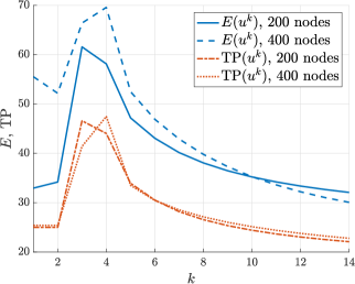
Figure 1. Instability accompanied by isotopy change for the inital curve defined in Section 4 with $\varkappa=1/10$ and $\varrho=1$ (case (b) in Table 1) and $\tau=\tfrac{1}{5}h_{\max}^{1/2}$. Top: snapshots and curve lengths for $h_{\max}\simeq 1/400$ after $k=1,2,3,4,6,8,10,16$ time steps (note different magnification); bottom: energy and self-avoidance potentials for $k=1,2,\dots,14$ with $h_{\max}\simeq 1/200$ and $h_{\max}\simeq 1/400$.

1  4  8  12   

12               13               14               15               16             

16   20  30  40

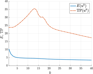
Figure 2. Energy stable evolution accompanied by an isotopy change for the inital curve defined in Section 4 with $\varkappa=1$ and $\varrho=1/100$ (case (e) in Table 1). Top: a self-penetration of the curve occurs after $14$ iterations; bottom: while the total energy decreases the tangent-point functional has a peak when the isotopy change takes place.

5. Simulating elastic knots

A primary goal in the experimental study of elastic knots is the determination of global minimizers of the energy functional $E$. As is typical for gradient flows and in particular for those related to singularly perturbed functionals, the evolution may become stationary at local minimizers or nearly stationary at so-called metastable states, see Carr and Pego [9] and Otto and Reznikoff [26]. In some cases small perturbations of the iterates can avoid these phenomena.

In this section we report on experiments targeted at the approximation of elastic knots [14] as global minimizers of $E$ when $\varkappa\gg\varrho$. In all cases, the evolution reaches some “stationary state” after finite time which seems to be a stable configuration. In general, it is difficult to decide whether it is in fact a local minimum, without even being a global minimum. Experiments with physical wires suggest the existence of several non-global local minimizers.

	# nodes	$h_{\max}$	pert.	$\ell_{\mathrm{ini}}$	$\ell_{\mathrm{end}}$
5.1	$376$	$0.1255$	yes	46.863580	46.855587
5.2 (a)	$401$	$0.1312$	no	49.996110	49.999110
5.2 (b)	$401$	$0.1312$	yes	49.996110	49.997392
5.3 (a)	$400$	$0.1370$	yes	49.871712	49.864798
5.3 (b)	$415$	$0.1306$	yes	49.884779	49.878556

Table 2. Discretization parameters for experiments defined in Subsections 5.1–5.3, we always use $\tau=\tfrac{1}{30}{h_{\max}}$ and $\varepsilon=2h_{\max}$.

Throughout this section we use $\varkappa=1$, $\varrho=10^{-3}$, and $q=3.9$ to define $E$. The discretization parameters used for the experiments defined below are listed in Table 2 where we use the same notation as in Section 4. The entries in the “pert.” column indicate whether a slight randomized perturbation was performed every hundred steps. The parameters $\ell_{\mathrm{ini}}$ and $\ell_{\mathrm{end}}$ denote the length of the curve at the initial step and the last step of the evolution respectively, more precisely, the length of the polygonal curve defined by the vertices.

Our general observation is that owing to the extreme ratio $\varkappa/\varrho=10^{4}$ one has to suitably choose the discretization parameters in order to prevent self-intersections during the evolution. For all experiments reported below the moderate number of approximately $400$ nodes and the relation $\tau=\frac{1}{30}h_{\max}$ were found to be sufficient.

5.1. Unknot

We experiment with an initial configuration proposed by Avvakumov and Sossinsky [1], consisting of a polygon describing a unilateral triangle with “twisted vertices”. The discrete evolution is depicted along with an energy plot in Figure 3 and we observe that the algorithm gets stuck in a configuration different from the global minimizer which is the round circle, cf. [14].

It is likely that this is an analytical feature of the gradient flow (3) and not an artifact of the numerical scheme. Therefore, at least for small values of $\varrho>0$, the gradient flow (3) does not seem to be a candidate for a retract of the unknots to the round circle (which exists due to the Smale conjecture, see Hatcher [18]).

1            100            200            300          

400            500            600            700          

800            900            1000            23000          

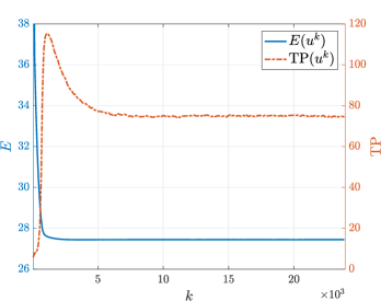
Figure 3. Numerical experiment with an unknot configuration defined in Section 5.1. Top: snapshots after $k=1,100,\dots,1000,23000$ iterations; bottom: monotonically decreasing energy curve. The discrete gradient flow starting from an unknotted symmetric polygon does not converge to the global minimizer, i.e., the round circle, but to a configuration which, being stable under small random perturbations, is likely to be a local minimizer.

5.2. Trefoil

In our second example we highlight the impact of symmetry to the evolution. The fact that a curve belonging to the trefoil knot class converges to a doubly covered circle (as predicted in [14]) has already been observed for the discretized $L^{2}$ gradient flow in [5].

Here we start with an embedded curve belonging to the trefoil knot class which is close to the three times covered circle. The initial curve is obtained by discretizing and rescaling the curve

(23) $$x\mapsto\begin{pmatrix}(2+0.1\cos(4\pi x))\cos(6\pi x)\\ (2+0.1\cos(4\pi x))\sin(6\pi x)\\ 0.1\sin(4\pi x)\end{pmatrix}.$$

The unperturbed discrete gradient flow (a) is depicted in the top part of Figure 4 and unfolds the curve but seems to get stuck in a conformation approximating the shape of two tangential circles tangentially meeting in an angle of $180$ degrees which might be a saddle point.

The perturbed discrete gradient flow (b) is depicted in the bottom part of Figure 4 and leaves that state after some time and approaches the shape of the elastic knot, i.e., the doubly covered (round) circle. The final energy value is quite close to the analytically predicted threshold of $\tfrac{\varkappa}{2}\cdot 50\cdot\left(\frac{4\pi}{50}\right)^{2}=\frac{(4\pi)^{2}}{10}\approx 15.79$, cf. [14].

The two evolutions are almost identical for the first 20,000 iteration steps. Here the snapshots shown in the top and bottom parts of Figure 4 show essentially the same configurations from different viewpoints, and the corresponding parts of the energy plot coincide as shown in Figure 5.

1  1000  2000  3000 

5000  6000  10000  12000 

14000                           15000                           20000                           80000                          

1  1000  2000  3000 

5000  10000  15000  20000 

25000  30000  35000  40000 

45000  50000  60000  80000 

Figure 4. Snapshots of the unperturbed (top) and perturbed (bottom) discrete evolutions for the initial trefoil configuration defined in Section 5.2. The unpertubed evolution becomes (experimentally) stationary in a symmetric but not energy minimizing configuration. Small perturbations lead to a different evolution after approximately 25,000 steps with a stationary configuration approximating a doubly covered circle that is globally energy minimizing.

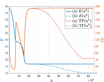
Figure 5. Energy curves for the (a) unperturbed and (b) perturbed discrete evolutions for the initial configuration defined in Section 5.2. The curves are nearly identical up to step 25,000 when the unperturbed evolution becomes stationary as depicted in Figure 4.

5.3. Figure-eight

Our third example illustrates how different initial configurations within one knot class lead to different stationary configurations and thereby show the limitations of gradient flows to determine particular representatives of a given class.

So far, there are no analytical results concerning the elastic figure-eight. Numerical experiments carried out by Gallotti and Pierre-Louis [13] as well as by Gerlach et al. [14] led to a spherical configuration exhibiting a remarkable symmetry (as the final state shown in the top part of Figure 6). Avvakumov and Sossinsky [1] instead claim that a planar configuration (as in the bottom part of Figure 6) yields a lower energy value compared to the spherical curve which they consider being merely a local minimizer. Our experiments indicate some support for the latter observation.

We retrieved coordinates of knotted curves from the website [28], namely (a) mseq-coord/3.html and (b) coord/3.html. In order to produce suitable initial curves, we added further nodes by cubic interpolation, performed a few iteration steps including some small randomized perturbation in order to allow for smoothing, and then rescaled the curve to a length of $50$ units.

The resulting configuration was taken as the initial curve for the respective experiment which again involved performing small randomized perturbations each hundredth step in order to break symmetry. The discrete evolutions are shown in Figures 6. The corresponding energy plots can be found in Figure 7.

1  100  200  300 

400  500  1000  2000 

3000  4000  5000  10000 

15000  20000  25000  40000  

1  100  200 

300  400  500 

1000                                         2000                                         40000                                        

Figure 6. Snapshots of two different discrete evolutions defined by initial configurations (a) and (b) specified in Section 5.3 within the figure-eight class leading to spherical (top) and planar (bottom) stationary configurations.

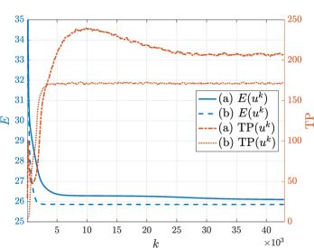
Figure 7. The energy plots for the evolutions defined by the initial configurations (a) and (b) in Section 5.3 (top and bottom parts of Figure 6) give rise to assuming that the stationary configuration obtained in (b) could be the global minimizer in the figure-eight class.

Acknowledgments

Philipp Reiter was partially supported by DFG-Grant RE 3930/1--1. The work on this manuscript was initiiated during the workshop ‘‘Geometric curvature functionals and discretizations’’ organized by Heiko von der Mosel which took place in Kloster Steinfeld in September 2017.

References

- [1] S. Avvakumov and A. Sossinsky. On the normal form of knots. Russ. J. Math. Phys., 21(4):421--429, 2014.
- [2] J. W. Barrett, H. Garcke, and R. Nürnberg. Parametric approximation of isotropic and anisotropic elastic flow for closed and open curves. Numer. Math., 120(3):489--542, 2012.
- [3] S. Bartels. A simple scheme for the approximation of the elastic flow of inextensible curves. IMA J. Numer. Anal., 33(4):1115--1125, 2013.
- [4] S. Bartels, Ph. Falk, and Ph. Reiter. KNOTevolve -- a tool for relaxing knots and inextensible curves. In preparation, 2018.
- [5] S. Bartels, Ph. Reiter, and J. Riege. A simple scheme for the approximation of self-avoiding inextensible curves. IMA Journal of Numerical Analysis, page drx021, 2017.
- [6] S. Blatt. The energy spaces of the tangent point energies. J. Topol. Anal., 5(3):261--270, 2013.
- [7] S. Blatt and Ph. Reiter. Regularity theory for tangent-point energies: the non-degenerate sub-critical case. Adv. Calc. Var., 8(2):93--116, 2015.
- [8] G. Buck and J. Orloff. A simple energy function for knots. Topology Appl., 61(3):205--214, 1995.
- [9] J. Carr and R. L. Pego. Metastable patterns in solutions of . Comm. Pure Appl. Math., 42(5):523--576, 1989.
- [10] A. Dall’Acqua, C.-C. Lin, and P. Pozzi. Evolution of open elastic curves in subject to fixed length and natural boundary conditions. Analysis (Berlin), 34(2):209--222, 2014.
- [11] K. Deckelnick and G. Dziuk. Error analysis for the elastic flow of parametrized curves. Math. Comp., 78(266):645--671, 2009.
- [12] G. Dziuk, E. Kuwert, and R. Schätzle. Evolution of elastic curves in : existence and computation. SIAM J. Math. Anal., 33(5):1228--1245, 2002.
- [13] R. Gallotti and O. Pierre-Louis. Stiff knots. Phys. Rev. E (3), 75(3):031801, 14, 2007.
- [14] H. Gerlach, Ph. Reiter, and H. von der Mosel. The elastic trefoil is the doubly covered circle. Arch. Ration. Mech. Anal., 225(1):89--139, 2017.
- [15] O. Gonzalez and J. H. Maddocks. Global curvature, thickness, and the ideal shapes of knots. Proc. Natl. Acad. Sci. USA, 96(9):4769--4773, 1999.
- [16] M. Gromov. Homotopical effects of dilatation. J. Differential Geom., 13(3):303--310, 1978.
- [17] M. Grothaus and N. Marheineke. On a nonlinear partial differential algebraic system arising in the technical textile industry: analysis and numerics. IMA J. Numer. Anal., 36(4):1783--1803, 2016.
- [18] A. E. Hatcher. A proof of the Smale conjecture, . Ann. of Math. (2), 117(3):553--607, 1983.
- [19] T. Hermes. Analysis of the first variation and a numerical gradient flow for integral Menger curvature. PhD thesis, RWTH Aachen University, 2012.
- [20] J. Langer and D. A. Singer. Curve straightening and a minimax argument for closed elastic curves. Topology, 24(1):75--88, 1985.
- [21] C.-C. Lin and H. R. Schwetlick. On a flow to untangle elastic knots. Calc. Var. Partial Differential Equations, 39(3-4):621--647, 2010.
- [22] A. Manhart, D. Oelz, C. Schmeiser, and N. Sfakianakis. An extended filament based lamellipodium model produces various moving cell shapes in the presence of chemotactic signals. J. Theoret. Biol., 382:244--258, 2015.
- [23] M. G. Mora and S. Müller. Derivation of the nonlinear bending-torsion theory for inextensible rods by -convergence. Calc. Var. Partial Differential Equations, 18(3):287--305, 2003.
- [24] J. O’Hara. Family of energy functionals of knots. Topology Appl., 48(2):147--161, 1992.
- [25] J. O’Hara. Energy of knots and conformal geometry, volume 33 of Series on Knots and Everything. World Scientific Publishing Co., Inc., River Edge, NJ, 2003.
- [26] F. Otto and M. G. Reznikoff. Slow motion of gradient flows. J. Differential Equations, 237(2):372--420, 2007.
- [27] P. Pozzi and B. Stinner. Curve shortening flow coupled to lateral diffusion. Numer. Math., 135(4):1171--1205, 2017.
- [28] R. Scharein. The knot server, 2003. Webpage, accessed 24 November 2017.
- [29] S. Scholtes. Discrete knot energies. ArXiv e-prints, Mar. 2016.
- [30] H. Schumacher. Pseudogradient flows of geometric energies. In preparation, 2018.
- [31] P. Strzelecki and H. von der Mosel. Tangent-point self-avoidance energies for curves. J. Knot Theory Ramifications, 21(5):1250044, 28, 2012.
- [32] H. von der Mosel. Minimizing the elastic energy of knots. Asymptot. Anal., 18(1--2):49--65, 1998.
- [33] M. Wardetzky, M. Bergou, D. Harmon, D. Zorin, and E. Grinspun. Discrete quadratic curvature energies. Comput. Aided Geom. Design, 24(8-9):499--518, 2007.