Theory of energy spectra in superfluid He-4 counterflow turbulence

Abstract

In the thermally driven superfluid ⁴He turbulence, the counterflow velocity $U_{\text{ns}}$ partially decouples normal and superfluid turbulent velocities. Recently we suggested [J. Low Temp. Phys. 187, 497 (2017)] that this decoupling should tremendously increase the turbulent energy dissipation by mutual friction and significantly suppress the energy spectra. Comprehensive measurements of the apparent scaling exponent $n_{\text{exp}}$ of the 2${}^{\text{nd}}$-order normal fluid velocity structure function $S_{2}(r)\propto r^{n_{\text{exp}}}$ in the counterflow turbulence [Phys.Rev.B 96, 094511 (2017)] confirmed our scenario of gradual dependence of the turbulence statistics on flow parameters. We develop an analytical theory of the counterflow turbulence, accounting for a two-fold mechanism of this phenomenon: i) a scale-dependent competition between the turbulent velocity coupling by mutual friction and the $U_{\text{ns}}$-induced turbulent velocity decoupling and ii) the turbulent energy dissipation by mutual friction enhanced by the velocity decoupling. The suggested theory predicts the energy spectra for a wide range of flow parameters. The mean exponents of the normal fluid energy spectra $\left\langle m\right\rangle_{\text{10}}$, found without fitting parameters, qualitatively agree with the observed $n_{\text{exp}}+1$ for $T\gtrsim 1.85\,$K.

Introduction

Below Bose-Einstein condensation temperature $T_{\lambda}\approx 2.17\,$K, liquid ⁴He becomes a quantum inviscid superfluid Donnely ; DB98 ; 2 . The vorticity in superfluid ⁴He is constrained to vortex-line singularities of core radius $a_{0}\approx 10^{-8}\,$cm and fixed circulation $\kappa=h/M$, where $h$ is Planck’s constant and $M$ is the mass of the ⁴He atomFeynman . The superfluid turbulence takes form of a complex tangle of these vortex lines, with a typical inter-vortex distanceVinen $\ell\sim 10^{-4}-10^{-2}\,$cm.

Large-scale hydrodynamics of such system can be described by a two fluid model, interpreting ⁴He as a mixture of two coupled fluid components: a superfluid with zero viscosity and a viscous normal fluid. The contributions of the components to the mixture are defined by their densities $\rho_{\text{s}},\rho_{\text{n}}:\rho_{\text{s}}+\rho_{\text{n}}=\rho$. Here $\rho$ is the density of ⁴He. The components are coupled by a mutual friction force, mediated by the tangle of quantum vortexes Donnely ; Vinen ; Vinen2 ; Vinen3 ; 37 .

There is a growing consensusSS-2012 ; TenChapters ; BLR that large-scale turbulence in mechanically driven superfluid ⁴He is similar to classical “Kolmogorov” turbulence. In this case, both components move in the same direction and the mutual friction force couples them almost at all scales. In this “coflowing” quasi-classical superfluid ⁴He Kolmogorov turbulence, the energy is supplied to the turbulent velocity fluctuations by large-scale instabilities, and is dissipated at small scales (below so-called Kolmogorov microscale) by viscous friction. Perhaps its most important property is a step-by step energy transfer over scales with a constant ($k$-independent) energy flux $\varepsilon(k)=$const. in the intermediate (or “inertial”) interval of scales.

The superfluid turbulence, called ultra-quantum or Vinen’s turbulence, may be excited in ⁴He directly at scales of the order of $\ell$, for example, by short pulses of electron beamGolov . In this case, there is no large-scale fluid motion. The tangle energy is dissipated by the mutual friction in the processes of vortex reconnections. During reconnection, sharp vortex tip causes very fast motion the vortex lines, that cannot be followed by the normal-fluid component due to its large inertia. The energy spectrum of of such a turbulence have a form of the peak with a maximum around $k_{\text{max}}\sim\pi/\ell$. Here, the energy is pumped and dissipated at the same scale and there is no energy flux over scales: $\varepsilon(k)=0$.

In discussions of the energy spectra of superfluid turbulence in ⁴He, the “Kolmogorov turbulence” is often contrasted with the “ultra-quantum” turbulence as two only forms of the energy transfer in the superfluids. However, we note that hydrodynamic turbulence in superfluid ³He, mechanically driven at large scales, can be considered as a third type of superfluid turbulence. In this case, the normal-fluid component can be considered laminar (or resting) due to its very large kinematic viscosity. The energy cascade toward small scales is accompanied by energy dissipation at all scales caused by the mutual friction. Therefore the energy flux $\varepsilon(k)$ is not constant, as in the Kolmogorov turbulence, and is not zero, as in Vinen’s turbulence, but is a decreasing function of $k$.

There is one more, unique way to generate turbulence in superfluid ⁴He in a channel. When a heater is located at a closed end of a channel, while another end is open to a superfluid helium bath, the heat flux is carried away from the heater by the normal fluid alone. To conserve mass, a superfluid current arises in the opposite direction. Here both components move relative to the channel walls with respective mean velocities ${\bm{U}}_{\text{n}}$ and ${\bm{U}}_{\text{s}}$. In this way a counterflow velocity ${\bm{U}}_{\text{ns}}={\bm{U}}_{\text{n}}-{\bm{U}}_{\text{s}}\neq 0$, proportional to the applied heat flux, is created along the channel, giving rise to a tangle of vortex lines.

Systematic studies of counterflow turbulence have more than half of a century history, going back to classical 1957-papers of VinenVinen3 . Due to experimental limitations these studies were mostly concentrated on global characteristics of the superfluid tubulence, such as $U_{\text{ns}}$-dependence of the intervortex distance, $\ell(U_{\text{ns}})$, [cf. reviews SS-2012 ; BLR ], the time evolution of the vortex-line-densityGolov1 ; Golov2 ; Vinen4 and similar. The statistics of turbulent fluctuations was inaccessible. Only few years ago, with the development of breakthrough experimental visualization techniques, the studies of the turbulent statistics of the normalWG-2015 ; WG-17a ; WG-17b and superfluidPrague1 ; Prague2 components in the ⁴He counterflow become possible.

In particular, using thin lines of the triplet-state He₂ molecular tracers created by a femptosecond-laser field ionization of He atoms 18 ; WG-2015 ; WG-17a , one can measure the streamwise normal velocity across a channel, $v_{x}(y,t)$ and extract the transversal 2${}^{\text{nd}}$-order structure functions

$$S_{2}(r)=\left\langle|\delta_{r}v_{x}(y,t)|^{2}\right\rangle\,,\ \delta_{r}v_{x}(y,t)\equiv v_{x}(y+r,t)-v_{x}(y,t)\,,$$

of the velocity differences $\delta_{r}$. Here $\left\langle\dots\right\rangle$ is a “proper” averaging: over $y$, ensemble of visualization pulses and time (in the stationary regime) or over ensemble at fixed time delay after switching off the heat flux. The physical meaning of $S_{2}(r)$ is the kinetic energy of turbulent velocity fluctuations (eddies, for shortness) of a scale $r$. For example, $S_{2}(r)\propto r^{n}$ means that the energy of eddies of size $r$ scales as $r^{n}$.

Another way to characterize the energy distribution in the one-dimensional (1D) wavenumber $k$-space is 1D energy spectrum $E(k,t)$, normalized such that the energy density per unit mass is defined as

$$E(t)=\frac{1}{2V}\int\left\langle|{\bm{u}}({\bm{r}},t)|^{2}\right\rangle d{\bm{r}}=\int\limits_{0}^{\infty}E(k,t)dk\,,$$ (1)

where $V=\int d{\bm{r}}$ is the system volume.

In the scale-invariant situation, such as the inertial interval of scales in the classical hydrodynamic isotropic turbulence, $E(k)\propto k^{-m}$. In this case, $S_{2}(r)$ may be reconstructed from $E(k)$ (up to irrelevant for us dimensionless prefactor) as follows:

$$S_{2}(r)=\int\limits_{0}^{\infty}E(k)\Big{[}1-\frac{\sin(k\,r)}{k\,r}\Big{]}dk\ .$$ (2a)

If $$E(k)\propto k^{-m} m 1<m<3 n m$$ and belongs to a so-called “window of locality”LP-95 , the integral (2a) converges and exponents and are related:

$$n=m-1\ .$$ (2b)

For example, Kolmogorov-1941 (K41) dimensional reasoning gives $m_{\scriptscriptstyle\rm{K41}}=\frac{5}{3}$ (falls within the window of locality) and simultaneously $n_{\scriptscriptstyle\rm{K41}}=\frac{2}{3}$, in agreement with Eq. (2b).

First measurementsWG-2015 of $S_{2}(r)$ in the ⁴He counterflow at $T=1.83\,$K found that $S_{2}(r)\propto r$ (i.e. $n=1$) instead of its K41 value $n_{\scriptscriptstyle\rm{K41}}=\frac{2}{3}$:

$$\mbox{K41:}\ S_{2}(r)\propto r^{2/3}\ \Rightarrow\ ^{4}\mbox{He:}\ S_{2}(r)\propto r\ .$$ (3a)

Using the relation Eq. (2b), the normal-fluid energy spectrum was reconstructed in LABEL:WG-2015 as

$$^{4}\mbox{He:}\ E_{\scriptscriptstyle\rm{He4}}(k)\propto k^{-2}\ .$$ (3b)

Observations (3), with an integer scaling exponent, stimulated attempts to clarify a possible “simple” underlying physical mechanisms. For example, based on the similarity of the spectrum (3b) with the Kadomtsev-Petviashvili spectrum KP of the energy spectrum of strong acoustic turbulence, $E(k)\propto k^{-2}$, (cf. Online lecture course FNP ) one may think that the ⁴He spectrum (3b) originates from (possible) discontinuities of the normal and superfluid velocities $v_{x}$ at planes, orthogonal to the counterflow direction ${\bm{\hat{x}}}$. Indeed, in the presence of randomly distributed velocity discontinuities, their contribution to the $S_{2}(r)$ is proportional to their number between two space points, separated by $r$, i.e. $S_{2}(r)\propto r$, as reported in LABEL:WG-2015.

However, to the best of our knowledge, no analytical reasons or numerical justifications for these discontinuities were not found so far. On the contrary, the developed analytic approachdecoupling ; BLPSV-2016 ; LP-2017 to the problem of turbulent statistics of ⁴He counterflow suggested a different scenario of this phenomenon. It was showndecoupling that in the counterflow turbulence, the normal and superfluid turbulent velocity fluctuations $u_{\text{n}}$ and $u_{\text{s}}$ become increasingly statistically independent (decoupled) as their scale decreases. This decoupling is due to sweeping of the normal fluid eddies by the mean normal fluid velocity $U_{\text{n}}$, while the superfluid eddies are swept by the mean superfluid velocity $U_{\text{s}}$ in the opposite direction. Therefore small scale normal fluid and superfluid eddies do not have enough time to be correlated by the mutual friction. This counterflow-induced decoupling significantly increases the energy dissipation by mutual friction, leadingBLPSV-2016 ; LP-2017 to a dependence of the turbulent statistics on the counterflow velocity. To what respect the scenarioLP-2017 reflects some (if any) aspects of the turbulent statistics in counterflow was an open question.

Recently, systematic experimental studiesWG-17a of the counterflow turbulence statistics in a wide range of temperatures $T$ and counterflow velocities $U_{\text{ns}}$ were carried out. The normal velocity structure functions $S_{2}(r)$ were found to have scaling behavior $S_{2}(r)\propto r^{n}$ in an interval of scales about one decade with an apparent scaling exponent that depends on both $U_{\text{ns}}$ and $T$, varying from about 0.9 to 1.4.

A first qualitative attempt to understand theoretically the underlying physics of these new results, was undertaken already in LABEL:WG-17a. Main physical ideas, used in this approach, largely overlap with those of the Weizmann groupdecoupling ; LNV ; BLPP-2012 ; BKLPPS-2017 ; LP-2017 , but are developed differently.

In this paper we offer a semi-quantitative theory of a stationary, space-homogeneous isotropic counterflow turbulence in superfluid ⁴He for a wide range of temperatures $T$ and counterflow velocities $U_{\text{ns}}$. The theory clarifies the details of complicated interplay between competing mechanisms of the turbulent velocity coupling by mutual friction and the $U_{\text{ns}}$-induced turbulent velocity decoupling, which, in addition, facilitates the turbulent energy dissipation by the mutual friction. Our main results are the turbulent energy spectra $E_{\text{n}}(k)$ and $E_{\text{s}}(k)$ of the normal and superfluid components of ⁴He in the wide range of the governing parameters: the temperature, the counterflow velocity, the vortex line density and Reynolds numbers. In particular, we demonstrate that the counterflow turbulence in ⁴He can be considered as the most general form of superfluid turbulence that manifests characteristic features of all three types of turbulence, discussed above:
(i) the quasi-classical Kolomogov-like turbulence with a constant energy flux at scales $r$ that exceed some cross-over scale $r_{\times}$, with both fluid components well coupled by mutual friction;
(ii) the ³He-like turbulence at scales $\ell<r<r_{\times}$, at which the normal- and superfluid components become decoupled and the turbulent energy is dissipated by the mutual friction during energy cascade toward small scales, similar to ³He turbulence with decreasing energy flux;
(iii) the ultra-quantum Vinen’s turbulence with the energy spectrum peak at the intervortex scale $\ell$ and no energy flux.

The paper is organized as follows:

In Sec. I we develop our analytical theory of the energy spectra in counterflow superfluid ⁴He turbulence. Our approach is based on the coarse-grained Hall-Vinen-Bekarevich-KhalatnikovHV ; BK equations of motion for the normal and superfluid turbulent velocities, summarized in Sec. I.1. In Sec. I.2 we derive the balance equations for the normal and superfluid turbulent energy spectra $E_{\text{n}}(k)$ and $E_{\text{s}}(k)$. In Sec. I.3 we suggest an important improvement to the algebraic closure: the self-consistent differential closure, that connects the energy fluxes over scales, $\varepsilon_{\text{n}}(k)$ and $\varepsilon_{\text{s}}(k)$ with the corresponding energy spectra $E_{\text{n}}(k)$ and $E_{\text{s}}(k)$ and their $k$-derivatives. The crucial component of the theory, the cross-correlation function of the normal and superfluid velocitiesdecoupling , is introduced in Sec. I.4. In the following Secs. I.5 and I.6 we formulate a simplified dimensionless version of the energy balance Eq. (18), which is central to our current approach.

We present the results of the numerical solution of Eq. (18) in a wide range of parameters ($T,U_{\text{ns}},{\mathcal{L}}$, Re) in Sec. II and analyze them in details in Secs. II.1–II.3. This allows us to clarify how three underlying physical processes: i) the turbulent velocity coupling by the mutual friction, characterized by a frequency $\Omega_{\text{ns}}$ (11d), ii) the velocity decoupling by counterflow velocity and iii) the energy dissipation by mutual friction, are competing. As a result of this competition, $E_{\text{n}}(k)$ and $E_{\text{s}}(k)$ have complicated behavior (cf. Fig. 1). In particular, we show that while the spectra are suppressed compared to the classical K41-spectrum at all scales, the degree of this suppression is scale-dependent: at small scales, the counterflow spectrum is less suppressed for larger $\Omega_{\text{ns}}$, while at larger scales the suppression becomes stronger with increasing $\Omega_{\text{ns}}$. The crossover scale, $k_{\times}$, depends on both $\Omega_{\text{ns}}$ and $U_{\text{ns}}$ such that the resulting spectra are not scale-invariant (cf. Figs.2 and 3). Note that all results, discussed above, are related to the quasi-classical energy spectra of turbulent motion with the scales $r$ much larger than the intervortex distance $\ell$. In Sec. II.4 we consider the presumed quantum peak in the superfluid energy spectra, clarifying its intensity with respect to the quasi-classical part of the superfluid spectra. Our important result is that the quasi-classical and quantum parts of the superfluid spectra are well separated in the wave-number space, see Fig. 5.

In Sec. II.5 we apply out theory to the range of parameters, similar to those realized in LABEL:WG-17a. To this end, we first discuss and estimate in Sec. II.5.1 the dimensionless parameters ${\rm Re}_{j},\widetilde{\Omega}_{\text{ns}}$ and $\widetilde{U}_{\text{ns}}$ that determine, according to our theory, the energy spectra. These parameters for 11 experimental conditions at four temperatures $T=1.65\,\ 1.85,\ 2.0\,$K and $T=2.1\,$K, are collected in Tab.2. The resulting pairs of normal- and superfluid energy spectra are shown in Fig. 6. The relation between experimental apparent scaling exponents $n_{\text{exp}}$ of the 2${}^{\text{nd}}$-order structure and the theoretical apparent scaling exponents of the energy spectra are discussed in Sec. II.5.2.

Finally, we summarize our findings. We discuss the restrictions and simplifications, used in our theory, and delineate possible directions of further development. In particular, we connect the discrepancy between theoretical and experimental scaling exponents at low temperatures with the possible influence of the space inhomogeneity of the counterflow turbulence in a channel at low Reynolds numbers, which is not accounted for in our theory.

I Energy balanced eqution

I.1 Gradually damped HVBK-equations for counterflow ⁴He turbulence

Following LABEL:DNS-He4,LP-2017,BKLPPS-2017, we describe the large scale turbulence in superfluid ⁴He by the gradually-damped versionHe4 of the coarse-grained Hall-Vinen HV -Bekarevich-KhalatnikovBK (HVBK) equations, generalized in LABEL:decoupling for the counterflow turbulence. In these equations the superfluid vorticity is assumed continuous, limiting their applicability to large scales with characteristic scale of turbulent fluctuations $R>\ell$. HVBK equations have a form of two Navier-Stokes equations for the turbulent velocity fluctuations ${\bm{u}}_{\text{n}}({\bm{r}},t)$ and ${\bm{u}}_{\text{s}}({\bm{r}},t)$:

$$\hskip-36.98866pt\frac{\partial\,{\bm{u}}_{\text{s}}}{\partial t}+[({\bm{u}}_{\text{s}}+{\bm{U}}_{\text{s}})\cdot{\bm{\nabla}}]{\bm{u}}_{\text{s}}-\frac{1}{\rho_{\text{s}}}{\bm{\nabla}}p_{\text{s}}=\nu_{\text{s}}\,\Delta{\bm{u}}_{\text{s}}+{\bm{f}}_{\text{ns}}\,,$$

$$\hskip-36.98866pt\frac{\partial\,{\bm{u}}_{\text{n}}}{\partial t}+[({\bm{u}}_{\text{n}}+{\bm{U}}_{\text{n}})\cdot{\bm{\nabla}}]{\bm{u}}_{\text{n}}-\frac{1}{\rho_{\text{n}}}{\bm{\nabla}}p_{\text{n}}=\nu_{\text{n}}\,\Delta{\bm{u}}_{\text{n}}-\frac{\rho_{\text{s}}}{\rho_{\text{n}}}{\bm{f}}_{\text{ns}}\,,$$

$$\hskip-36.98866ptp_{\text{n}}=\frac{\rho_{\text{n}}}{\rho}[p+\frac{\rho_{\text{s}}}{2}|{\bm{u}}_{\text{s}}-{\bm{u}}_{\text{n}}|^{2}]\,,p_{\text{s}}=\frac{\rho_{\text{s}}}{\rho}[p-\frac{\rho_{\text{n}}}{2}|{\bm{u}}_{\text{s}}-{\bm{u}}_{\text{n}}|^{2}]\,,$$

$${\bm{f}}_{\text{ns}} \simeq \Omega_{\text{s}}\,({\bm{u}}_{\text{n}}-{\bm{u}}_{\text{s}})\,,\quad\Omega_{\text{s}}=\alpha(T)\kappa{\mathcal{L}}\,,$$ (4b)

coupled by the mutual friction force ${\bm{f}}_{\text{ns}}$ in the form (4b), suggested in LABEL:LNV. It involves the turbulent velocity fluctuations of the normal- and superfluid components, the temperature dependent dimensionless dissipative mutual friction parameter $\alpha(T)$ and the superfluid vorticity $\kappa{\mathcal{L}}$, defined by the vortex line density ${\mathcal{L}},\,\ell={\mathcal{L}}^{-1/2}$.

Other parameters entering Eqs. (4) include the pressures $p_{\text{n}}$, $p_{\text{s}}$ of the normal and the superfluid components, the total density $\rho\equiv\rho_{\text{s}}+\rho_{\text{n}}$ of ⁴He and the kinematic viscosity of normal fluid component $\nu_{\text{n}}=\eta/\rho_{\text{n}}$ with $\eta$ being the dynamical viscosityDB98 of normal ⁴He component. The dissipative term with the Vinen’s effective superfluid viscosity $\nu_{\text{s}}$ Vinen was added in LABEL:He4 to account for the energy dissipation at the intervortex scale $\ell$ due to vortex reconnections, the energy transfer to Kelvin waves and similar effects.

Generally speaking, Eqs. (4) involve also contributions of a reactive (dimensionless) mutual friction parameter $\alpha^{\prime}$, that renormalizes the nonlinear terms. For example, in Eq. (4) $({\bm{u}}_{\text{s}}\cdot{\bm{\nabla}}){\bm{u}}_{\text{s}}\Rightarrow(1-\alpha^{\prime})({\bm{u}}_{\text{s}}\cdot{\bm{\nabla}}){\bm{u}}_{\text{s}}$. However, in the studied range of temperatures $|\alpha^{\prime}|\lesssim 0.02\ll 1$ and this renormalization can be ignored. For similar reasons we neglected all other $\alpha^{\prime}$-related terms in Eqs. (4).

I.2 General energy balance equations

Our theory is based on the stationary balance equations for the 1D energy spectra $E_{\text{n}}(k)$ and $E_{\text{s}}(k)$ of the normal and superfluid components, defined by Eq. (1).

To derive these equations, Eqs. (4) were Fourier transformed, multiplied by the complex conjugates of the corresponding velocities and properly averaged. The pressure terms were eliminated using the incompressibility conditions. Finally, the energy balance equations have a form:

$$\frac{d\varepsilon_{j}}{dk}=\Omega_{j}\big{[}E_{\text{ns}}(k)-E_{j}(k)\big{]}-2\,\nu_{j}k^{2}E_{j}(k)\ .$$ (5)

Here we use subscript “_j” to denote either superfluid or normal fluid $j\in\{\mbox{s, n}\}$ and define $\Omega_{\text{n}}=\Omega_{\text{s}}\rho_{\text{s}}/\rho_{\text{n}}$. The normal-fluid-superfluid cross-correlation function $E_{\text{ns}}(k)$ is defined similarly to Eq. (1):

$$E_{\text{ns}}=\frac{1}{2V}\int\left\langle{\bm{u}}_{\text{n}}({\bm{r}},t)\cdot{\bm{u}}_{\text{s}}({\bm{r}},t)\right\rangle d{\bm{r}}=\int\limits_{0}^{\infty}E_{\text{ns}}(k)\,dk\ .$$ (6)

The energy transfer term $d\varepsilon_{j}/dk$ in Eq. (5) originates from the nonlinear terms in the HVBK Eqs. (4) and has the same formLP-95 ; LP-2 ; BL as in classical turbulence:

$$\frac{d\varepsilon_{j}(k)}{dk} = 2\,\mbox{Re}\Big{\{}\int V^{\xi\beta\gamma}({\bm{k}},{\bm{q}},{\bm{p}})\,F_{j}^{\xi\beta\gamma}({\bm{k}},{\bm{q}},{\bm{p}})$$ (7a)

$$\times\delta({\bm{k}}+{\bm{q}}+{\bm{p}})\frac{d^{3}q\,d^{3}p}{(2\pi)^{6}}\,\Big{\}}\,,$$

$$V^{\xi\beta\gamma}({\bm{k}},{\bm{q}},{\bm{p}}) = i\Big{(}\delta_{\xi\xi^{\prime}}-\frac{k^{\xi}k^{\xi^{\prime}}}{k^{2}}\Big{)}$$ (7b)

$$\times\Big{(}k^{\beta}\delta_{\xi^{\prime}\gamma}+k^{\gamma}\delta_{\xi^{\prime}\beta}\Big{)}\ .$$

Here $F_{j}^{\xi\beta\gamma}({\bm{k}},{\bm{q}},{\bm{p}})$ is the simultaneous triple-correlation function of turbulent (normal or superfluid) velocity fluctuations in the ${\bm{k}}$-representation, that we will not specify here and $V^{\xi\beta\gamma}({\bm{k}},{\bm{q}},{\bm{p}})$ is the interaction vertex in the HVBK (as well as in the Navier-Stokes) equations. Importantly, the right-hand-side of Eq. (7a) conserves the total turbulent kinetic energy (i.e. the integral of $E_{j}(k)$ over entire ${\bm{k}}$-space) and therefore can be written in the divergent form as ${d\varepsilon_{j}}/{dk}$.

I.3 Self-consistent differential closure

One of the main problems in the theory of hydrodynamic turbulence is to find the triple-correlation function $F^{\xi\beta\gamma}({\bm{k}},{\bm{q}},{\bm{p}})$, which determines the energy flux $\varepsilon(k)$ in Eqs. (7). The simplest way is to directly model $\varepsilon(k)$ using dimensional reasoning to connect $\varepsilon(k)$ and the energy spectrum $E(k)$ with the same wavenumber $k$:

$$\varepsilon(k)=Ck^{5/2}E^{3/2}(k)\,,$$ (8)

Here $C$ is the phenomenological constant with the value $C\approx 0.5$, corresponding to the fully developed turbulence of classical fluid CK ; YeungZhou . The algebraic closure (8) is basedFri mainly on the Kolmogorov-1941 (K41) assumption of the universality of turbulent statistics in the limit of large Reynolds numbers and on the Richardson-1922 step-by-step cascade picture of the energy transfer towards large $k$. The energy-cascade picture combined with the K41 idea that in this case $\varepsilon(k)$ is the only relevant physical parameter determining the level of turbulent excitations and their statistics, lead to Eq. (8).

More realistic modeling of $\varepsilon(k)$ can be reached in the framework of integral closures, widely used in analytic theories of classical turbulenceFri , for example, so-called Eddy-damped quasinormal Markovian (EDQNM) closure or Kraichnan’s Direct Interaction Approximation Kra1 ; Kra2 . These closures are based on the representation of third-order velocity correlation function $F^{\xi\beta\gamma}_{\text{s}}$ in Eq. (7a) as a product of the vertex $V$, Eq. (7b), two second-order correlations $E(k)$, and the response (Green’s) functions $G(k)\sim\Gamma(k)-$the typical relaxation frequencies at scale $k$. Keeping in mind the uncontrolled character of integral closures, L’vov, Nazarenko and Rudenko (LNR) suggested in LABEL:LNR a simplified version of EDQNM closure with the same level of justification for isotropic turbulence. LNR replaced a volume element [$d^{3}q\,d^{3}p\,\delta^{3}({\bm{k}}+{\bm{q}}+{\bm{p}})$] in Eq. (7a), involving 3-dimensional vectors ${\bm{k}}$, ${\bm{q}}$, and ${\bm{p}}$, by its isotropic version [$q^{2}dq\,p^{2}dp\ \delta(k+q+p)/(k^{2}+q^{2}+p^{2})$], involving only one-dimensional vectors $k$, $q$, and $p$ varying over the interval $(-\infty,+\infty)$. In addition, they replaced the interaction amplitude $V^{\xi\beta\gamma}({\bm{k}},{\bm{q}},{\bm{p}})$, Eq. (7b) by its scalar version $(ik)$. The resulting LNR closure can be written as follows:

$$\frac{d\varepsilon(k)}{dk}=\frac{A_{1}\,k}{2\pi^{2}}\int_{-\infty}^{\infty}\frac{dq\,dp\,\delta(k+q+p)}{2\pi\,(k^{2}+q^{2}+p^{2})}$$ (9a)

$$\hskip-14.22636pt\times\frac{k^{3}\,E(|q|)E(|p|)+q^{3}\,E(|k|)E(|p|)+p^{3}\,E(|q|)E(|k|)}{\Gamma(|k|)+\Gamma(|q|)+\Gamma(|p|)}\ .$$

Here $$A_{1}$$ is a dimensionless parameter of the order of unity.

The integral closure (9a) may be related to the algebraic closure (8) by assuming that the integral (9a) converges (i.e. the main contribution to it comes from the wavenumbers of similar scales $q\sim p\sim k$, so-called locality of interaction) and estimating $\Gamma(k)$ as $\sqrt{k^{3}E(k)}$ and $d\varepsilon(k)/dk$ as $\varepsilon(k)/k$.

The LNR model (9a) satisfies all the general closure requirements: i) it conserves energy, $\int\frac{d\varepsilon(k)}{dk}dk=0$ for any $E(k)$; ii) $\frac{d\varepsilon(k)}{dk}=0$ for the thermodynamic equilibrium spectrum $E(k)\propto k^{2}$ and for the cascade K41 spectrum $E(k)\propto|k|^{-5/3}$. Importantly, the integrand in Eq. (9a) has the correct asymptotic behavior in the limits of small and large $q/k$, as required by the sweeping-free Belinicher-L’vov representation BL . This means that the model (9a) adequately reflects the contributions of the extended-interaction triads and thus can be used for the analysis of the non-local energy transfer, which become importantBKLPPS-2017 when the scaling exponent $m$ approaches $m=3$.

The mutual friction terms in Eqs. (4) cause additional energy dissipation at all scales. Therefore, we can expect that the energy spectra may be steeper than K41 and not scale-invariant.

To generalize the closure (9a) for such a situation, assume that the energy spectrum has a form $E(k)=E_{0}/k^{m}$ with a scaling exponent $m\geqslant 5/3$. As $m\to 3$, the main contribution to the integral (9a) comes from the distant interactions with wavevectors of different scales. In particular, the $\delta$-function in the integral dictates that for $q\ll k$, $p\approx-k$ and the integral (9a) may be approximated as:

$$\frac{d\varepsilon(k)}{dk} \approx \frac{A_{1}\,E_{0}}{8\pi^{3}k\Gamma(|k|)}\int_{-k}^{k}\frac{dq}{q^{m}}$$ (9c)

$$\times\big{[}k^{3}\,E(|k+q|)-(k+q)^{3}E(k)\big{]}$$

$$\hskip-42.67912pt\approx\frac{A_{1}\,E_{0}}{8\pi^{3}k\Gamma(|k|)}\,\frac{d^{2}}{dq^{2}}\big{[}k^{3}\,E(|k+q|)-(k+q)^{3}E(k)\big{]}_{q\to 0}$$

$$\times\int\limits_{0}^{\infty}q^{2-m}dq\simeq\frac{A_{1}\big{[}kE(k)\big{]}^{3/2}}{8\pi^{3}(3-m)}\ .$$

Dimensionally, Eq. (9c) coincides with the K41 algebraic closure (8), but contains additional prefactor $1/(3-m)$. This may be interpreted as $m$-dependent parameter $C$ in front of Eq. (8), which diverges as $m\to 3$. The physical reason for such a dependence is simple: as $m$ increases, more and more extended triads that involve $k$- and $(q\ll k)$-modes contribute to the energy influx in the $k$-mode. As a result, the energy flux grows $\propto 1/(3-m)$, according to Eq. (9c). Moreover, when $m\geqslant 3$ the integral (9c) formally diverges, meaning that the leading contribution to the flux at $k$-mode comes not from comparable $(q\sim k)$-modes (as assumed in the Richardson-Kolmogorov step-by-step cascade picture of the energy flux), but directly from the largest, energy-containing modes in the turbulent flow.

Thus, by accounting for the possible scale-dependent nonlocal energy transfer over scales, we generalize the standard K41-closure (8) by including the $k$-dependence of the prefactor $C$:

$$\varepsilon(k)=C(k)k^{5/2}E^{3/2}(k)\,,\ C(k)=\frac{4\,C}{3\,[3-m(k)]}\ .$$ (10a)

For convenience, the prefactor $$C(k) C m(k)=5/3 m(k) E(k$$ is chosen to reproduce the Kolmogorov constant for the K41 scaling exponent . As follows from above arguments, the function of in (10a) should be understood as a local scaling exponent of ):

$$m(k)=\frac{d\ln E(k)}{d\ln(k)}\ ,$$ (10b)

making the new closure a self-consistent differential closure.

I.4 Cross-correlation function

The general form of the cross-correlation functiondecoupling $E_{\text{ns}}$ reads as:

$$E_{\text{ns}}(k) = D(k)E_{\text{ns}}^{(0)}(k)\,,\ D(k)=\frac{\arctan[\xi(k)]}{\xi(k)}\,,~{}~{}~{}~{}~{}~{}~{}~{}$$ (11a)

$$\ \xi(k) = \frac{k}{k_{\times}}\,,\quad k_{\times}=\frac{\Gamma(k)}{U_{\text{ns}}}\ .$$ (11b)

Here $$D(k) U_{\text{ns}} E_{\text{ns}}^{(0)}(k)$$ is the -dependent decoupling function, and has the formLNS ; He4 :

$$E_{\text{ns}}^{(0)}(k) = \frac{\Omega_{\text{ns}}\big{[}\rho_{\text{n}}E_{\text{n}}(k)+\rho_{\text{s}}E_{\text{s}}(k)\big{]}}{\Gamma(k)\,\rho}\,,$$ (11c)

$$\Gamma(k) = \Omega_{\text{ns}}+\gamma_{\text{s}}(k)+\gamma_{\text{n}}(k)+(\nu_{\text{s}}+\nu_{\text{n}})\,k^{2}\,,$$ (11d)

$$\Omega_{\text{ns}} = \Omega_{\text{n}}+\Omega_{\text{s}}=\alpha\kappa{\mathcal{L}}\frac{\rho}{\rho_{\text{n}}}\,,\ \gamma_{j}(k)=C_{\gamma}\sqrt{k^{3}E_{j}(k)}\ .~{}~{}~{}$$

Here $C_{\gamma}$ is a phenomenological parameter, the same for both components. However $E_{\text{n}}(k)$ and $E_{\text{s}}(k)$ in Eq. (11c) are not the energy spectra at $U_{\text{ns}}=0$, but the $U_{\text{ns}}$-dependent energy spectra, found self-consistently by solving Eqs. (5) with $E_{\text{ns}}(k)$ given by Eqs. (11).

$T$, K	1.4	1.65	1.85	1.95	2.0	2.1
$\rho_{\text{n}}/\rho$	0.0728	0.193	0.364	0.482	0.553	0.741
$\alpha$	0.051	0.111	0.181	0.236	0.279	0.481
$\alpha\rho/\rho_{\text{n}}$	0.701	0.575	0.497	0.489	0.504	0.649
$\nu_{\text{n}}/\kappa$	1.34	0.462	0.248	0.199	0.182	0.167
$\nu_{\text{s}}^{\prime}/\kappa$	0.135	0.228	0.265	0.296	0.312	0.427

Table 1: The parameters DB98 of the superfluid ⁴He: the normal component fraction $\rho_{\text{n}}/\rho$; the mutual friction parameter $\alpha$, the combination $\alpha\rho/\rho_{\text{n}}$ ; the kinematic viscosity of the normal-fluid component $\nu_{\text{n}}\equiv\mu/\rho_{\text{n}}$; the effective superfluid viscosity Vinen $\nu^{\prime}_{\text{s}}$.

I.5 Simplified energy balance equation

The Eqs. (5) are coupled via cross-correlation function $E_{\text{ns}}$, which depends on the energy spectra of both components. To find the leading contributions to $E_{\text{ns}}$, we recall that at $k$ close to $k_{0}$ the velocities are well correlateddecoupling , meaning that $E_{\text{n}}(k)\simeq E_{\text{s}}(k)$, while for $k\gg k_{0}$ they are almost decorrelated and $E_{\text{ns}}(k)$ is negligible compared to $E_{\text{n}}$ and $E_{\text{s}}$. Therefore, without loss of accuracy we can replace $E_{\text{n}}(k)$ by $E_{\text{s}}(k)$ in Eqs. (11) for $E_{\text{ns}}$ that enters into balance equation (5) for the superfluid and $E_{\text{s}}(k)$ by $E_{\text{n}}(k)$ for $E_{\text{ns}}$ that enters into normal-fluid balance equation.

In this way we obtain decoupled equations for the fluxes $\varepsilon_{\text{n}}$ and $\varepsilon_{\text{s}}$

$$\frac{d\varepsilon_{j}}{dk} = E_{j}(k)\big{\{}\Omega[D_{j}(k)-1]-2\,\nu_{j}k^{2}\big{\}}\,,$$ (12a)

with different decoupling functions for the normal-fluid and superfluid components:

$$D_{j}(k) = \frac{\Omega_{\text{ns}}\arctan[kU_{\text{ns}}/\Gamma_{j}(k)]}{kU_{\text{ns}}}\,,$$ (12b)

and different values of full damping frequencies:

$$\Gamma_{j}(k) = \Omega_{\text{ns}}+2C_{\gamma}\sqrt{k^{3}E_{j}(k)}+(\nu_{\text{s}}+\nu_{\text{n}})k^{2}\ .$$ (12c)

The balance Eqs. (12), being uncoupled for the normal-fluid and superfluid components, are already much simpler than the fully coupled balance equations (5) and (11).

We are now ready to make next step and to analyze the relative importance of different contributions to the damping frequencies $\Gamma_{j}(k)$, comparing the dissipation due to mutual friction $\Omega_{\text{ns}}$, the rate of the energy transfer between scales $C_{\gamma}\sqrt{k^{3}E(k)}$ and the viscous dissipation $(\nu_{\text{s}}+\nu_{\text{n}})k^{2}$. We start with $\Omega_{\text{ns}}=\alpha(T)\kappa{\mathcal{L}}\rho/\rho_{\text{n}}(T)$. In the intermediate range of temperatures $\alpha(T)\rho/\rho_{\text{n}}(T)\approx 0.5$, weakly depending on $T$, cf Tab. 1. Therefore we can peacefully take $\Omega_{\text{ns}}\approx 0.5\kappa{\mathcal{L}}$.

Next, the sum $(\nu_{\text{s}}+\nu_{\text{n}})$ in this temperature interval also weakly depends on $T$ and is very close to $0.5\,\kappa$. (cf. Tab. 1 and Fig. 5 in LABEL:He4 and LABEL:LSS for discussion on physical origin of the numerical value). Estimating the largest wavenumber of the inertial interval by the quantum cutoff $k_{\text{max}}\sim 1/\ell=\sqrt{{\mathcal{L}}}$, we find that $(\nu_{\text{s}}+\nu_{\text{n}})k_{\text{max}}^{2}\simeq 0.5\kappa{\mathcal{L}}\approx\Omega_{\text{ns}}$. Therefore, $(\nu_{\text{s}}+\nu_{\text{n}})k^{2}<\Omega_{\text{ns}}$ in the entire inertial interval, except for its large-$k$ end, where the accurate representation of the decoupling functions is not important. This allows us to neglect in most cases the viscous contributions in Eq. (12c) for $\Gamma_{j}(k)$.

To estimate the energy transfer terms, recall that in the classical K41 turbulence (with $E(k)\propto k^{-5/3}$) $\sqrt{k^{3}E(k)}$ grows as $k^{2/3}$. It remains larger than viscous terms in the entire inertial range and become compatible with $\nu k^{2}$ at the large-$k$ end of the inertial interval, at the Kolmogorov microscale. In our case, the spectra $E_{j}(k)$ decay with $k$ faster than the K41 spectrum, owing to the energy dissipation due to mutual friction. Therefore, in the inertial interval of counterflow turbulence $\sqrt{k^{3}E_{j}(k)}$ grows slower than in K41 turbulence and remains smaller than $\Omega_{\text{ns}}$ for all $k$. Moreover, recent estimate of $C_{\gamma}$ using Direct Numerical Simulations of the superfluid ⁴He turbulenceDNS-He4 gives $C_{\gamma}\ll 1$. Therefore, for these conditions we can neglect the energy transfer terms compared to $\Omega_{\text{ns}}$. Having all these in mind, we approximate $\Gamma_{j}$ as $\Omega_{\text{ns}}$ and, using Eq. (12b), get

$$D_{\text{n}}(k)=D_{\text{s}}(k)\equiv D(k)\,,$$ (13)

with $\xi(k)=kU_{\text{ns}}/\Omega_{\text{ns}}$.

Now, we combine Eqs. (10), (12a) and (13) to finalize an approximation for the balance equations

$$C(k)\,\frac{d}{dk}k^{5/2}E_{j}^{3/2}(k) = E_{j}(k)\big{\{}\Omega_{j}[D(k)-1]$$ (14a)

$$-2\nu_{j}k^{2}\big{\}},~{}~{}~{}~{}~{}~{}$$

$$D(k)=\frac{\arctan[\xi(k)]}{\xi(k)}\,, \quad\xi(k)=\frac{kU_{\text{ns}}}{\Omega_{\text{ns}}}\ .$$ (14b)

In deriving Eq. (14a) we neglected for simplicity the $k$-derivative of $m(k)$ in the expression for $C(k)$ with respect to $d[k^{5/3}E(k)]/dk$ since $m(k)$ varies between 5/3 to 3 in the entire range of $k$, while $k^{5/3}E(k)$ varies by many orders of magnitude.

I.6 Dimensionless form of the energy balance equation

To analyze the energy balance Eq. (14) and to open a way to its numerical solution, we first rewrite it in the dimensionless form. To this end we introduce a dimensionless wavenumber $q$ and a dimensionless energy spectrum ${\mathcal{E}}(q)$:

$$q=k/k_{0}\,,\quad{\mathcal{E}}(q)=E(k)/E(k_{0})\ .$$ (15)

Here the minimal wave number is estimated as $k_{0}=2\pi/\Delta$, where $\Delta$ is outer scale of turbulence.

The resulting dimensionless equations for new dimensionless functions

$$\Psi_{j}(q)=\sqrt{q^{5/3}{\mathcal{E}}_{j}(q)}\,,$$ (16a)

take the form

$$\frac{d\Psi_{j}(q)}{dq} = A_{j}\,\frac{D(qk_{0})-1}{q^{5/3}}-a_{j}\,q^{1/3}\,,~{}j\in\{s,n\}\,,~{}~{}~{}~{}$$ (16b)

$$A_{j} = \frac{\Omega_{j}}{3C(k)\sqrt{k_{0}^{3}E_{j}(k_{0})}}\,,$$ (16c)

$$\ a_{j} = \frac{2\nu_{j}\sqrt{k_{0}}}{3C(k)\sqrt{E_{j}(k_{0})}}\ .~{}~{}~{}~{}~{}$$ (16d)

To clarify further the parameters in Eqs. (16), we define the dimensionless parameters that govern the counterflow superfluid turbulence: the turbulent Reynolds numbers, the efficiency of dissipation by mutual friction and the dimensionless counterflow velocity.

Similar to the classical hydrodynamic turbulence, the energy dissipation by viscous friction in the superfluid turbulence is governed by the Reynolds number. There are two such Reynolds numbers, ${\rm Re}_{\text{n}}$ and ${\rm Re}_{\text{s}}$:

$${\rm Re\!}_{j}=\frac{u_{\scriptscriptstyle\rm{T}}}{k_{0}\nu_{j}}\,,\quad u_{\scriptscriptstyle\rm{T}}\simeq\sqrt{k_{0}E(k_{0})}\ .$$ (17a)

Here we ignore the presumably small difference between velocity fluctuations of the components at scale $$k_{0} E_{\text{s}}(k_{0})=E_{\text{n}}(k_{0})=E(k_{0}) u_{\scriptscriptstyle\rm{T}} \sqrt{k_{0}E(k_{0})} {\rm Re}_{\text{s}}/{\rm Re}_{\text{n}}=\nu_{\text{n}}/\nu_{\text{s}} {\rm Re}_{\text{n}}$$ [i.e assume ] and estimate the root-mean-square (rms) turbulent fluctuations as . The ratio of the Reynolds numbers (17a) is defined by the viscosities and depends only on the temperature. Therefore, for a given temperature we are left with only one Reynolds number, say .

There is one more mechanism of the energy dissipation in superfluid turbulence: the dissipation by mutual friction. This kind of dissipation is characterized by the frequency $\Omega_{\text{ns}}$, Eq. (11c). As was mentioned above, $\Omega_{\text{ns}}\approx 0.5\kappa{\mathcal{L}}$ in the entire temperature range. Then, the partial frequencies $\Omega_{\text{s}}$ and $\Omega_{\text{n}}$ that govern the energy dissipation by mutual friction in the superfluid and normal-fluid components with a given $\Omega_{\text{ns}}$, depend only on the densities $\rho_{\text{s}}$ and $\rho_{\text{n}}$, according to Eq. (11c). Therefore we can say that for a given temperature, the dissipation by mutual friction is governed by only one frequency $\Omega_{\text{ns}}\propto{\mathcal{L}}$.

As was shown in Refs. LNV ; BLPP-2012 ; BKLPPS-2017 , the rate of energy dissipation by mutual friction should be compared with the $k$-dependent rate of the energy transfer over the cascade, characterized by the turnover frequency of the eddies of scale $1/k$, $\gamma_{j}(k)$, Eq. (11c). This dictates a natural normalization of $\Omega_{\text{ns}}$ by $\gamma(k_{0})$, which can be estimated as $k_{0}u_{\scriptscriptstyle\rm{T}}$. In other words, we suggest to use

$$\widetilde{\Omega}_{\text{ns}}\equiv\Omega_{\text{ns}}/k_{0}u_{\scriptscriptstyle\rm{T}}\,,$$ (17b)

as the dimensionless parameter that characterizes the efficiency of dissipation by mutual friction .

Last important parameter of the problem is the counterflow velocity $U_{\text{ns}}$. It is natural to normalize it by the turbulent velocity $u_{\scriptscriptstyle\rm{T}}$, introducing a dimensionless velocity

$$\widetilde{U}_{\text{ns}}\equiv U_{\text{ns}}/u_{\scriptscriptstyle\rm{T}}\,,$$ (17c)

Using parameters (17) together with Eqs. (10) and (14b) we rewrite Eq. (16) as follows

$$4C\,\frac{d\Psi_{j}}{dq} = -\Big{[}\frac{2}{3}+\frac{d\Psi_{j}}{dq}\,\frac{q}{\Psi_{j}}\Big{]}$$

$$\times\Big{\{}\frac{\widetilde{\Omega}_{j}}{q^{5/3}}\Big{[}1-\frac{\arctan(q/q_{\times})}{q/q_{\times}}\Big{]}+\frac{2}{\mbox{Re}_{j}}\Big{\}}$$

$$\widetilde{\Omega}_{\text{n}}=\widetilde{\Omega}_{\text{ns}}\frac{\rho_{\text{s}}}{\rho}\,, \widetilde{\Omega}_{\text{s}}=\widetilde{\Omega}_{\text{ns}}\frac{\rho_{\text{n}}}{\rho}\,,\quad q_{\times}=\frac{\widetilde{\Omega}_{\text{ns}}}{\widetilde{U}_{\text{ns}}}\ .$$ (18b)

These are the first-order ordinary differential equations for $\Psi_{j}(q)$. Aside from the temperature dependent parameter $\rho_{\text{n}}/\rho$, they include four dimensionless parameters that characterize the superfluid counterflow turbulence: $\widetilde{\Omega}_{\text{ns}}$, $\widetilde{U}_{\text{ns}}$ and Re_j.

$T=1.65\,$K, $\ \widetilde{U}_{\text{ns}}=1.0$	$T=1.65\,$K,  $\widetilde{U}_{\text{ns}}=4.0$	$T=1.65\,$K,  $\widetilde{U}_{\text{ns}}=8.0$
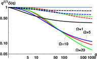
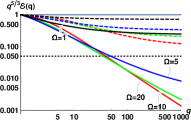
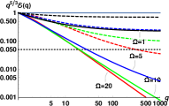
$T=1.85\,$K, $\ \widetilde{U}_{\text{ns}}=1.0$	$T=1.85\,$K,  $\widetilde{U}_{\text{ns}}=4.0$	$T=1.85\,$K,  $\widetilde{U}_{\text{ns}}=8.0$
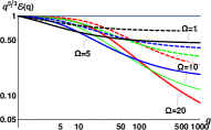
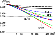
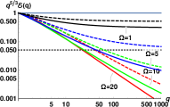
$T=1.95\,$K, $\ \widetilde{U}_{\text{ns}}=1.0$	$T=1.95\,$K,  $\widetilde{U}_{\text{ns}}=4.0$	$T=1.95\,$K,  $\widetilde{U}_{\text{ns}}=8.0$
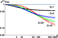
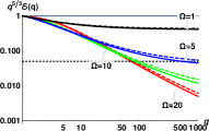
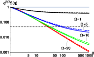
$T=2.10\,$K, $\ \widetilde{U}_{\text{ns}}=1.0$	$T=T=2.10\,$K,  $\widetilde{U}_{\text{ns}}=4.0$	$T=T=2.10\,$K,  $\widetilde{U}_{\text{ns}}=8.0$

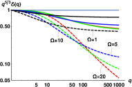
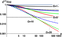
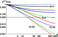
Figure 1: Color online. The compensated energy spectra ${\mathcal{E}}_{j}(q)=q^{5/3}E_{j}(q)/E_{j}(q_{0})$ vs $q=k/k_{0}$ for ${\rm Re}_{j}=\infty$ and different combinations of $T$ and $\tilde{U}_{\text{ns}}$. The lines corresponding to different values of $\widetilde{\Omega}_{\text{ns}}$ are shown by different colors (from top to bottom): $\widetilde{\Omega}=0$ (the horizontal gray lines), $\widetilde{\Omega}_{\text{ns}}=1.0$ (black lines), $\widetilde{\Omega}_{\text{ns}}=5.0$ (blue lines), $\widetilde{\Omega}_{\text{ns}}=10.0$ (green lines) and $\widetilde{\Omega}_{\text{ns}}=20.0$ (the lowest red lines). The normal-fluid energy spectra are shown by solid lines, the superfluid spectra – by dashed lines. Note that in the left column $q^{5/3}{\mathcal{E}}_{j}(q)$ varies from 0.05 to 1.0, while in the middle and the right columns – from 0.01 to 1.0. In these panels the level 0.05 is shown by the horizontal dotted lines. The labels ”$\Omega$“ in the figures mark one of the lines of the corresponding color (solid or dashed) for further clarity.

$\widetilde{U}_{\text{ns}}=1$	$\widetilde{U}_{\text{ns}}=4$ K	$\widetilde{U}_{\text{ns}}=8$

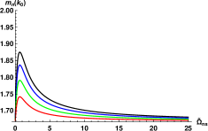
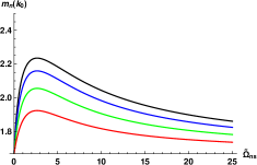
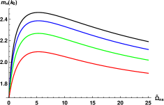
Figure 2: Color online.The outer-scale scaling exponents of the normal component $m_{\text{n}}(1)$ [Eq. (19)] vs. $\widetilde{\Omega}_{\text{ns}}$ for $\widetilde{U}_{\text{ns}}=1$ (left panel), $\widetilde{U}_{\text{ns}}=4$ (middle panel) and $\widetilde{U}_{\text{ns}}=8$ (right panel). The lines from top to bottom correspond to $T=1.65\,$K (black lines), $T=1.85\,$K (blue lines), $T=2.0\,$K (green lines), and $T=2.10\,$K (red lines).

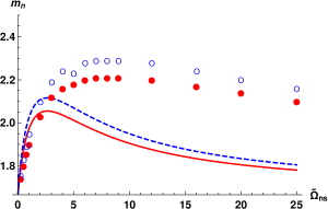
Figure 3: Color online. The $\widetilde{\Omega}_{\text{ns}}$ dependence of the scaling exponents $m_{j}(1)$ and the mean exponent $\left\langle m_{j}\right\rangle_{10}$. The normal component exponent $m_{\text{n}}(1)$ is marked as red solid line, $\left\langle m_{\text{n}}\right\rangle_{10}$ –by red full circles. The superfluid exponent $m_{\text{s}}(1)$ is marked by blue dashed line, the mean exponent $\left\langle m_{\text{s}}\right\rangle_{10}$ – by empty blue circles. The exponents were calculated for $T=2.0\,$K and $\widetilde{U}_{\text{ns}}=4$.

II Energy spectra of counterflow turbulence

II.1 Qualitative analysis of the energy spectra

To qualitatively analyze the energy spectra, we first neglect in Eqs. (18) the influence of the viscous dissipation. In Fig. 1 we show the energy spectra, obtained by solving Eq. (18) in a wide range of dimensionless parameters with Re${}_{\text{s,n}}\to\infty$. In all panels, the normal component spectra are shown by solid lines and the superfluid component spectra – by dashed lines.

Each row represent the spectra at one of four temperatures, from top to bottom: $T=1.65,1.85,1.95$ and $2.1$K.

The three columns show solutions for three different values of the dimensionless counterflow velocity (17c): $\widetilde{U}_{\text{ns}}=1$ (left), $\widetilde{U}_{\text{ns}}=4$ (middle) and $\widetilde{U}_{\text{ns}}=8$ (right).

Each of the panels contains the spectra for 5 values of the dimensionless frequency $\widetilde{\Omega}_{\text{ns}}$ from 0 (the horizontal gray lines) to $\tilde{\Omega}_{\text{ns}}=20$ (the lowest red lines), color-coded as described in the figure caption.

Comparing spectra shown in Fig. 1, we can make a set of observations:

i) The larger the counterflow velocity $\widetilde{U}_{\text{ns}}$, the stronger is the suppression of the energy spectra compared to the K41 prediction. This is an expected result: the normal-fluid and superfluid velocity fluctuations decorrelate faster with increasing $\widetilde{U}_{\text{ns}}$, leading to stronger energy dissipation by mutual friction and as a result– to a more prominent suppression of the energy spectra.

ii) In the absence of viscous dissipation, the dissipation by mutual friction defines the suppression of the spectra. The corresponding frequencies $\Omega_{j}$ [Eq. (18b)], are proportional to the other component’s densities: $\Omega_{\text{s}}\propto\rho_{\text{n}},\Omega_{\text{n}}\propto\rho_{\text{s}}$. Therefore, at low temperatures (two upper rows), when $\rho_{\text{n}}\ll\rho_{\text{s}}$, the normal-fluid component spectra are suppressed stronger than the superfluid spectra, while at high $T$ the relation is reversed (the lowest row).

iii) The competition between the velocity fluctuations coupling and the dissipation due to mutual friction leads to a complicated $q$-dependence of the spectra, described by Eq. (12a): the rate of energy dissipation is proportional to $\Omega_{j}[D_{j}(q)-1]$. The larger is $\Omega_{j}$ the stronger is the coupling, however, simultaneously $D_{j}(q)\to 1$. Which factor wins, depends on the scale: at large $q$ the dissipation wins and the spectra suppression is directly proportional to $\widetilde{\Omega}_{j}$. On the other hand, at small $q$, the spectra for larger $\widetilde{\Omega}_{j}$ are less suppressed, especially at weak counterflow velocity.

Note that the applicability range of HVBK [Eqs. (4)] is limited by $k<\pi/\ell=\pi\sqrt{{\mathcal{L}}}\simeq\pi\sqrt{2\Omega_{\text{ns}}/\kappa}$. However our analysis is performed for given values of $\widetilde{\Omega}_{\text{ns}}=\Omega_{\text{ns}}/k_{0}u_{\text{T}}$ with $k_{0}=1$ and an arbitrary value of $u_{\scriptscriptstyle\rm{T}}$. Therefore, there is no formal restriction on the range of $k$ in Figs. 1, (as well as in Figs. 2, 3, and Fig. 4), which was chosen as to expose all important features of the energy spectra.

$T=1.65\,$K	$T=1.95\,$K	$T=2.10\,$K

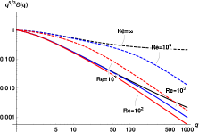
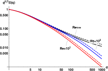
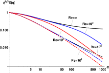
Figure 4: Color online. The viscous corrections to the energy spectra at different temperatures: $T=1.65\,$K (left panel), $T=1.95\,$K (middle panel) and $T=1.21\,$K (right panel). The norma-fluidl spectra are shown by solid lines, the superfluid spectra – by dashed lines. The spectra are shown for Re${}_{\text{n}}=\infty$ (black lines), Re${}_{\text{n}}=10^{3}$ (blue lines) and $10^{2}$ (red lines). All spectra were calculated with $\widetilde{U}_{\text{ns}}=4$ and $\widetilde{\Omega}_{\text{ns}}=10$.

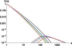
Figure 5: Color online. The (uncompensated) energy spectra of counterflow turbulence, ${\mathcal{E}}_{\text{s}}(q)=E(q)/E(q_{0})$ vs $q=k/k_{0}$ (dashed lines) and the sketch of the quantum peak (dot-dashed lines) for $T=1.65\,$K, $Q=300\,$mW/cm² (upper black lines) $T=1.85\,$K, $Q=497\,$mW/cm² (blue lines) $T=2.00\,$K $Q=586\,$mW/cm² (green lines) and $T=2.10\,$K $Q=350\,$mW/cm² (lowest red lines). Note that here the $q$-range, where ${\mathcal{E}}_{\text{s}}(q)$ are valid, is limited by $q\lesssim 200$.

II.2 Outer-scale and mean scaling exponents of the energy spectra

To characterize in a compact form the energy spectra dependence on the flow parameters, $T$, $\widetilde{U}_{\text{ns}}$ and $\widetilde{\Omega}_{\text{ns}}$, we consider first a scaling exponent $m(q)$, Eq. (10b), in the beginning of the scaling interval $k=k_{0},q=1$. Using Eqs. (16a) and (18) we get for outer-scale exponent $m_{j}(q=1)$:

$$m_{j}(1)=\frac{5}{3}+\frac{4}{3}\,\frac{\widetilde{\Omega}_{j}\big{[}1-q_{\times}\arctan(1/q_{\times})\big{]}}{4C+\widetilde{\Omega}_{j}\big{[}1-q_{\times}\arctan(1/q_{\times})\big{]}}\,.~{}~{}~{}~{}~{}$$ (19)

The $\widetilde{\Omega}_{\text{ns}}$-dependencies of the normal-fluid outer-scale exponent $m_{n}(1)$ for different $\widetilde{U}_{\text{ns}}$ and $T$ are shown in Fig. 2. As expected, for $\widetilde{\Omega}_{\text{ns}}=0$ (no mutual friction damping) $m_{\text{n}}(1)=\frac{5}{3}$, the classical K41 value. In the limit $\widetilde{\Omega}_{\text{ns}}\to\infty$, $\displaystyle\lim_{q_{\times}\to\infty}[q_{\times}\arctan(1/q_{\times})]\propto 1/q_{\times}^{2}$ and $m_{\text{n}}(1)$ again tends to its K41 value $\frac{5}{3}$. In this limit, the normal and superfluid components are fully coupled and there is no energy dissipation by mutual friction. The resulting $\widetilde{\Omega}_{\text{ns}}$-dependence of $m_{n}(q)$ is non-monotonic with a maximum around $\widetilde{\Omega}_{\text{ns}}\sim 1$. As we saw before, the $m_{n}(1)$ is largest (i.e. the strongest suppression of normal-fluid energy spectra) at lowest $T=1.65\,$K (upper black lines), the smallest – at high $T=2.1\,$K (the lowest red lines).

Conversely, the superfluid exponents $m_{s}(1)$ (not shown) reflect strong suppression [larger $m_{s}(1)$] at high temperatures, while at low temperatures $m_{s}(1)$ are smaller.

To characterize the degree of deviation from the scale invariance, we introduce the mean scaling exponent over some $q$-interval from $q=1$ [with ${\mathcal{E}}_{j}(1)=1$] to a given value of $q$ :

$$\left\langle m_{j}\right\rangle_{q}=-\ln{\mathcal{E}}_{j}(q)\big{/}\ln q\ .$$ (20)

The value $\left\langle m_{j}\right\rangle_{q}$ should be $q$-independent and equal to the outer-scale exponent $m_{j}(1)=[d\ln{\mathcal{E}}_{j}(q)/d\ln q]_{q=1}$ for the scale-invariant spectra and vary otherwise. In Fig. 3 we compare $m_{j}(1)$ and $\left\langle m_{j}\right\rangle_{10}$ for $T=2.0$K and $\widetilde{U}_{\text{ns}}=4$. The outer-scale scaling exponent $m_{\text{n}}(1)$ is shown by solid line, $m_{\text{s}}(1)$ – by dashed line. The values of $\left\langle m_{\text{n}}\right\rangle_{10}$ and $\left\langle m_{\text{s}}\right\rangle_{10}$, calculated for a set of $\widetilde{\Omega}_{\text{ns}}$, are shown by full and empty circles, respectively. Clearly, the spectra coincide (at least within the first decade) for $\widetilde{\Omega}_{\text{ns}}\lesssim 3$, while for stronger $\widetilde{\Omega}_{\text{ns}}$ they vary significantly: the actual spectra are more suppressed than is suggested by $m_{j}(1)$ and $\left\langle m_{j}\right\rangle_{10}>m_{j}(1)$ for $\widetilde{\Omega}_{\text{ns}}>3$ at this temperature. The non-monotonic behavior is evident in all curves, although the maximum in the mean exponents $\left\langle m_{j}\right\rangle_{10}$ is broader and less prominent.

II.3 Viscous damping of the energy spectra

Having in mind the influence of $\widetilde{\Omega}_{\text{ns}}$ and $\widetilde{U}_{\text{ns}}$ on the energy spectra, we now add the viscous dissipation to the picture and plot in Fig. 4 the compensated spectra for $T=1.65,\ 1.95\,$ and $T=2.10\,$K, using $\widetilde{U}_{\text{ns}}=4$ and $\widetilde{\Omega}_{\text{ns}}=10$. The spectra for Re${}_{\text{n}}\to\infty$ are shown by black lines, those for Re${}_{\text{n}}=10^{3}$– by blue lines, while red lines denote the spectra for Re${}_{\text{n}}=10^{2}$. The corresponding Re${}_{\text{s}}$ were calculated using the ratio of viscosities (cf. Table 1).

As expected, the reduction of Re_j leads to progressive damping of the energy spectra. This effect is mostly concentrated at large $q$, while at small $q$ the energy dissipation by mutual friction dominates. The viscous damping is most prominent for the denser component (superfluid at $T=1.65$K and normal fluid at $T=2.1$K). At $T=1.95\,$K, the densities of the components are close and the spectra are similar for all Re numbers.

II.4 Quantum peak in superfluid energy spectra

As has long been known Vinen3 and understood Schwarz that besides large scale turbulence, discussed above, the intense counterflow generates the superfluid turbulence (the vortex tangle). The corresponding energy spectra peak at the intervortex scale $\ell=1/\sqrt{{\mathcal{L}}}$. This kind of superfluid turbulence has no classic analog and is traditionally called Vinen’s or ultra-quantum turbulence.

The total energy density of quantum turbulence (per unit mass of superfluid component) $E_{\scriptscriptstyle\rm{Q}}$ may be reasonably estimated within the Local Induction ApproximationSchwarz as

$$E_{\scriptscriptstyle\rm{Q}}=\frac{\kappa^{2}{\mathcal{L}}\Lambda}{2\pi}\,,\quad\Lambda\approx\ln(\ell/a_{0})\ .$$ (21a)

Here $$a_{0} \sim 10^{-8}\, {\mathcal{L}}\simeq 10^{5} \Lambda\approx 12.6 {\mathcal{L}}$$ is the vortex core radius (cm in ⁴He). For the typical value , and very weakly depends on . Therefore for our purposes we can estimate

$$E_{\scriptscriptstyle\rm{Q}}\simeq 2\,\kappa^{2}{\mathcal{L}}\ .$$ (21b)

Using experimental values of ${\mathcal{L}}$, discussed below, we found $E_{\scriptscriptstyle\rm{Q}}$ and compared them with $E_{\text{cl}}$, calculated for the experimental conditions. It is interesting to realize that $E_{\text{cl}}\sim E_{\scriptscriptstyle\rm{Q}}$. For example, at $T=1.65\,$K the ratio $E_{\scriptscriptstyle\rm{Q}}/E_{\text{cl}}$ varies between 1.2 and 1.8, for $T=2.00\,$K $E_{\scriptscriptstyle\rm{Q}}/E_{\text{cl}}\simeq 5$. This fact may be rationalized by simple models of turbulent channel flow (cf. e.g LABEL:Pope) and by dimensional reasoning. Indeed, for the classical channel flow, the dimensional reasoning (and simple models – up to logarithmic corrections) give $\Delta u_{\text{n}}\simeq U_{\text{ns}}$ as supported by the experiment [column # 8 of Tab. 2]. Thus $E_{\text{cl}}\simeq U_{\text{ns}}^{2}$.

For the quantum energy of superfluid turbulence, Eqs. (21b) gives $E_{\scriptscriptstyle\rm{Q}}\simeq 2\kappa^{2}{\mathcal{L}}$, while ${\mathcal{L}}=(\gamma U_{\text{ns}})^{2}$ with $\gamma\simeq 1/\kappa$. Therefore, also for the quantum energy $E_{\scriptscriptstyle\rm{Q}}\simeq U_{\text{ns}}^{2}$.

Our knowledge of quantum peak $k$-dependence, $E_{\scriptscriptstyle\rm{Q}}(k)$, is quite limited. Dimensional reasoning, supported by the numerical simulationsBaggaley2012 , predicts maximum of $E_{\scriptscriptstyle\rm{Q}}(k)$ at the inverse intervortex distance $k_{*}\simeq 2\pi\sqrt{{\mathcal{L}}}$. For $k_{*}\ll k<2\pi/a_{0}$, $E_{\scriptscriptstyle\rm{Q}}(k)$ is dictated by the velocity field near the vortex line: $v(r)\propto\kappa/r$, where $r$ is the distance to the vortex line. Modeling quantum vortex tangle as a set of randomly oriented vortex lines with the vortex line density ${\mathcal{L}}$ and averaging over line orientations, we get an asymptotic behavior $E_{\scriptscriptstyle\rm{Q}}(k)\simeq\kappa^{2}{\mathcal{L}}/k$ for $2\pi/a_{0}\gg k\gg k_{*}$. The same answer follows from dimensional reasoning based on a natural assumption that $E_{\scriptscriptstyle\rm{Q}}(k)\propto{\mathcal{L}}$.

For $k\ll k_{*}$ we do not expect inverse energy cascade in 3D turbulence. Therefore, following LABEL:BLPSV-2016, we assume here local thermodynamic equilibrium spectra with equipartition of energy between degrees of freedom: $E_{\scriptscriptstyle\rm{Q}}(k)\propto k^{2}$. Simple analytic formula that reflects all these properties has a form:

$$E_{\scriptscriptstyle\rm{q}}(k)=\frac{E_{\scriptscriptstyle\rm{Q}}}{\Lambda}\,\frac{k^{2}}{k_{*}^{3}+k^{3}}\,,\ k_{*}=\frac{2\pi}{\ell}\ .$$ (22a)

Here $$E_{\scriptscriptstyle\rm{Q}}$$ is the total energy of quantum peak,

$$E_{\scriptscriptstyle\rm{Q}}=\int_{0}^{2\pi/a_{0}}E_{\scriptscriptstyle\rm{Q}}(k)\,dk\ .$$ (22b)

Taking the values of $E_{\scriptscriptstyle\rm{Q}}$ and $\ell=1/\sqrt{{\mathcal{L}}}$ from the Tab. II, we plot in Fig. 5 the energy spectra, corresponding to the quantum-peak (22) for four temperatures (dot-dashed lines). We also show by dashed lines the quasi-classical superfluid energy spectra $E_{\text{s}}(k)$. We see that the quasi-classical and quantum parts of the superfluid energy spectra are well separated in the $k$-space, as was suggested in Refs. BLPSV-2016 ; Vinen for the explanation of the vortex line density decay ${\mathcal{L}}(t)$ after switching off the counterflow.

What is important for us now is that the distinct separation of the quasi-classical and quantum contributions to the superfluid energy spectra allows us to neglect the direct effect of the quantum peak on the behavior of the normal fluid and superfluid quasi-classical turbulence. The only role played by the quantum peak in our theory is to give an independent and leading contribution to the vortex-line density that determines the mutual friction.

II.5 Energy spectra in the conditions of the Tallahassee experiments

Now we are ready to analyze the energy spectra for conditions, close to realized in the ⁴He counterflow visualization experimentWG-17a .

The experimentsWG-17a ; WG-17b in the turbulent counterflow of superfluid ⁴He were conducted for a range of temperatures and heat fluxes. A number of important properties of the flow, required for comparison between theory and experiment are listed in Table 2.

The normal velocity fluctuations were deduced by the visualization of the molecular tracers WG-2015 ; WG-17a . The ratio of this turbulence intensity to the mean normal velocity is almost independent of the values of the heat flux for a given temperature WG-17a . The vortex line density ${\mathcal{L}}$ was measured by the second sound attenuation.

#	1	2	3	4	5	6	7	8	9	10	11	12	13
	$T,$	$Q,$	$U_{\text{n}},$	$u_{\scriptscriptstyle\rm{T}}$	${\cal L},$	${\rm Re}_{\text{n}}=$	${\rm Re}_{\text{s}}=$	$\widetilde{U}_{\text{ns}}=$	$\widetilde{\Omega}_{\text{ns}}=$	$E_{\text{cl}},$	$E_{\scriptscriptstyle\rm{Q}},$	$n_{\text{exp}}+1$	$\left\langle m_{\text{n}}\right\rangle_{\text{10 }}$
#	K	$\rm mW/cm^{2}$	cm/s	cm/s	cm-2	$u_{\scriptscriptstyle\rm{T}}/(k_{0}\nu_{\text{n}})$	$\ u_{\scriptscriptstyle\rm{T}}/(k_{0}\nu_{\text{s}})$	$\ U_{\text{ns}}/u_{\scriptscriptstyle\rm{T}}$	$\ \Omega_{\text{ns}}/(k_{0}u_{\scriptscriptstyle\rm{T}})$	cm2/s2	cm2/s2
1		150	1.87	0.5	8.63 $\times 10^{4}$	37.89	76.78	4.64	3.47	0.12	0.17	1.89$\pm 0.03$	2.48
2	1.65	200	2.23	0.61	16.2 $\times 10^{4}$	46.23	93.67	4.52	3.35	0.18	0.32	2.14$\pm 0.03$	2.47
3		300	3.27	1.12	38.2 $\times 10^{4}$	84.88	171.99	3.61	6.87	0.62	0.73	2.18$\pm 0.04$	2.43
4		200	1.18	0.38	8.11 $\times 10^{4}$	53.22	50.21	4.87	3.72	0.07	0.16	1.88$\pm 0.04$	2.41
5	1.85	300	1.78	0.67	19.8 $\times 10^{4}$	94.21	88.52	4.17	5.14	0.22	0.39	2.23$\pm 0.02$	2.38
6		497	3.03	1.17	58.5 $\times 10^{4}$	165.52	154.59	4.07	8.71	0.68	1.09	2.35$\pm 0.03$	2.37
7		233	0.86	0.44	14.1$\times 10^{4}$	84.65	51.01	4.37	5.66	0.096	0.28	2.3$\pm 0.02$	2.34
8	2.0	386	1.34	0.68	47.3$\times 10^{4}$	130.82	78.84	4.41	12.29	0.23	0.89	2.31$\pm 0.03$	2.32
9		586	2.09	1.16	112 $\times 10^{4}$	223.17	134.49	4.03	17.05	0.67	2.04	2.36$\pm 0.02$	2.23
10	2.1	200	0.57	0.51	37.3$\times 10^{4}$	106.93	41.82	4.31	16.62	0.13	0.71	2.09$\pm 0.02$	2.08
11		350	0.99	1.01	114$\times 10^{4}$	211.76	82.82	3.79	25.65	0.51	2.07	2.11$\pm 0.04$	1.96

Table 2: Columns ## 1–5: the experimental parameters of the flowWG-17a . Columns ## 6–9: the parameters of the model. In columns #10 and #11: $E_{\text{cl}}=(u_{\text{T}})^{2}/2$ and $E_{\text{Q}}\approx 2\kappa^{2}\,{\mathcal{L}}$. Columns #12 and #13: the experimental values of the apparent scaling exponent $n_{\text{exp}}+1$ , and the theoretical normal fluid mean exponents over first decade $\left\langle m_{\text{n}}\right\rangle_{\text{10}}$.

II.5.1 Measured and estimated parameters of the experiments

The experimentsWG-17a were performed at four temperatures $T=~{}1.65,1.85,2.0$ and $2.10\,$K using different values of the heat flux $Q$, ranging from 150 to $\sim 600\,$mW/cm². The measured values of the resulting mean normal fluid velocity $U_{\text{n}}$, the normal-fluid rms turbulent velocity fluctuation $u_{\scriptscriptstyle\rm{T}}$ and the vortex line densities ${\mathcal{L}}$ (columns #3-#5, Tab. 2) are reproduced according to Table I, LABEL:WG-17a.

Using these data and parameters of superfluid ⁴He for relevant temperatures, Tab. 1, we computed the “turbulent” Reynolds numbers Re_j and listed them in columns #6 and #7 of Tab. 2. We used a simplified assumption that at large, energy containing scales, the rms turbulent velocity fluctuations $u_{j}$ of the normal and superfluid components are close due their coupling by mutual friction: $u_{\text{s}}\approx u_{\text{n}}=u_{\scriptscriptstyle\rm{T}}$. As an estimate of the outer scale of turbulence we take $\Delta=0.225\,$cm which is a mean upper limit of the approximate scaling behavior of $S_{2}(r)$, measured in LABEL:WG-17a. Note that the values of Re_j in these experiments are quite low, with Re${}_{\text{n}}$ ranging from Re${}_{\text{n}}\simeq 38$ (line #1) to Re${}_{\text{n}}\simeq 223$ (line #9).

The counterflow velocity $U_{\text{ns}}=U_{\text{n}}-U_{\text{s}}$ was found from the measured mean normal-fluid velocity $U_{\text{n}}$ and the condition of zero mass flux.

Its resulting dimensionless values $\widetilde{U}_{\text{ns}}=U_{\text{ns}}/u_{\scriptscriptstyle\rm{T}}$ are given in the column #8.

The mutual-friction frequencies $\Omega_{\text{ns}}$ were calculated from Eq. (11d), using measured values of the VLD ${\mathcal{L}}$ and ⁴He parameters. The dimensionless values $\widetilde{\Omega}_{\text{ns}}$ are listed in the column # 9. They are ranging from $\approx 3.4$ for $T=1.65\,$K to $\approx 26$ for $T=2.10\,$K. We used the estimate $k_{0}\approx 2\pi/\Delta=28\,$ cm^-1.

II.5.2 The scaling behavior of the energy spectra and the 2${}^{\text{nd}}$ order structure function

The energy spectra for each of11 sets of measurements, computed using Eqs. (18) with the corresponding parameters, are collected in Fig. 6. At each temperature, the red lines correspond to the spectrum with the largest value of the heat flux $Q$, the green lines – for the intermediate value of $Q$ and the lowest blue lines – to the smallest $Q$. For these flow conditions, all spectra are strongly suppressed and are not scale-invariant, although the degree of the deviation from scale-invariance varies. Interestingly, at these conditions the normal fluid spectra for all temperatures, except $T=2.1\,$K, appear very similar to each other. To characterize the scaling behavior of these spectra, we use again Eq. (20) and calculate the mean exponents over first decade $\left\langle m_{\text{n}}\right\rangle_{\text{10}}$.

The scaling behavior of such non-scale-invariant spectra do not have simple relation to the scaling exponents of the second order structure function. The experimentally measured 2nd order transversal structure functions $S^{\bot}_{2}(r)$ were found to exhibit a power-law behavior over an interval of scales of about one decade. The examplesWG-17b of the experimental $S^{\bot}_{2}(r)$ for $T=1.85\,$K and different heat fluxes are shown in Fig. 7. The scaling exponents $n_{\text{exp}}$ were measured by a linear fit over the corresponding $r$-range and it was suggestedWG-17a that the scaling exponents of the underlying energy spectra should scale as $n_{\text{exp}}+1$. We therefore compare the theoretical predictions $\left\langle m_{\text{n}}\right\rangle_{\text{10}}$ with the proposed experimental exponents $n_{\text{exp}}+1$, listed in the columns #12 and #13, Tab.2. The error-bars for $n_{\text{exp}}+1$ correspond to the fit quality of $S^{\bot}_{2}(r)$. It was assumedWG-17a that additional experimental inaccuracies (supposedly present in previous experiments WG-2015 ) are absent.

(a) $T=1.65\,$K	(b) $T=1.85\,$K
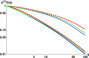
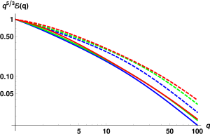
(c) $T=2.0\,$K	(d) $T=2.1\,$K

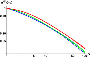
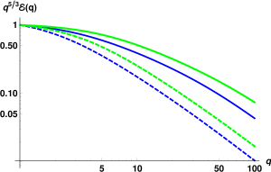
Figure 6: Color online. The compensated energy spectra for experimental conditions at $T=1.65$K [Panel(a)], $T=1.85$K [Panel(b)], $T=2.0$K [Panel(c)] and $T=2.1\,$K Panel (d)]. The spectra for large heat fluxes $Q$ are shown by red lines [upper lines in panels (a)-(c)], for moderate heat fluxes– by green lines and for small heat fluxes– by lower blue lines. The explicit values of $Q$ are given in Tab. 2. The normal fluid spectra are shown by solid lines, the superfluid spectra – by dashed lines. Note, that all spectra here are shown for $q<100$, within the applicability range of Eqs. (4) for the relevant flow parameters.

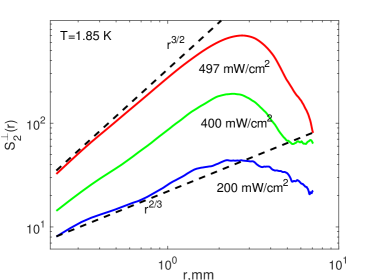
Figure 7: Color online. The 2-nd order structure functionsWG-17b $S_{2}(r)$ as a function of separation $r$ for $T=1.85\,$K and different heat fluxes. The black dashed lines indicate the scaling behavior $r^{2/3}$ and $r^{3/2}$ and serve to guide the eye only.

To rationalize the results, we first analyze the dimensionless model parameters, corresponding to the experimental conditions. First of all, the dimensionless counterflow velocity $\widetilde{U}_{\text{ns}}\approx 4$ for all conditions. Therefore, the differences in flow conditions for a given temperature are mostly translated to the differences in efficiency of the dissipation by mutual friction $\widetilde{\Omega}_{\text{ns}}$. As we saw in Figs. 2 and 3, in the relevant range $\widetilde{\Omega}_{\text{ns}}\simeq 3.5-26$, the mean scaling exponents $\left\langle m_{\text{n}}\right\rangle_{\text{10}}$ are expected to be strongly affected by the dissipation due to mutual friction and to weakly depend on $\widetilde{\Omega}_{\text{ns}}$. Indeed, for relatively large $\widetilde{\Omega}_{\text{ns}}$, the exponents $n_{\text{exp}}+1$ are clustered by temperatures and do not vary much. However, their values are smaller for $T=2.1\,$K than for $T=2.0\,$K, while exponents for $T=2\,$K and $T=1.85\,$K are compatible (except for the smallest heat flux, for which both the Re${}_{\text{n}}$ and $\widetilde{\Omega}_{\text{ns}}$ are small). This trend agrees with the expected $T$ dependence, shown in Fig. 2, if we also account for the difference in the Reynolds numbers (cf. Fig. 4). Remarkably, for these conditions the theoretical values of $\left\langle m_{\text{n}}\right\rangle_{\text{10}}$ are in a good qualitative agreement with $n_{\text{exp}}+1$. Note that these values were obtained without any fitting parameters. The discrepancy between experimental estimates and theoretical predictions is limited to the flows with low Reynolds numbers ($T=1.65$K and $T=1.85$K, $Q=200$mW/cm²). In these conditions, the flow inhomogeneity, not accounted for by our theory, may play important role. In particular, in the low Re channel flow, the width of the near-wall buffer layer is compatiblePope with the width of the turbulent core (the region of well-developed turbulence around the channel centerline). Its contribution to the velocity structure functions become significant. The typical size of the largest eddies in the buffer layer is not constant: it is of order of the local distance to the wall and smaller than the outer scale in the turbulent core. A more accurate estimate of $\Delta$ (or $k_{0}$, which defines the dimensionless model parameters) for these conditions, may improve the agreement between the theory and experiment. For instance, with all other parameters unchanged, larger $k_{0}$ leads to smaller $\widetilde{\Omega}_{\text{ns}}$. These smaller $\widetilde{\Omega}_{\text{ns}}$ correspond to the lower, fast-changing part of the $m$ vs $\widetilde{\Omega}_{\text{ns}}$ curves in Fig. 3. This kind of behavior is indeed observed at $T=1.65$K. The simplifications of the theory in the description of the energy exchange between components are another possible reason for the discrepancy at low $T$.

Conclusions

We developed a semi-quantitative theory of stationary, space-homogeneous isotropic developed counterflow turbulence in superfluid ⁴He. The theory captures basic physics of the energy spectra dependence on the main flow parameters and accounts for the interplay between:

(i) the turbulent velocity coupling by mutual friction, dominant at large scales $r>r_{\times}\simeq\pi/k_{\times}$;

(ii) its decoupling, caused by the sweeping of the normal and superfluid eddies in the opposite directions, which becomes important at scales $r<r_{\times}$;

(iii) the turbulent energy dissipation due to mutual friction at scales $r<r_{\times}$, that gradually decreases the energy flux over scales and suppresses the energy spectrum, similar to the turbulence in ³He.

The ultra-quantum peak, well separated from the quasi-classical interval of scales $r>\ell$, serves in our theory as a space- and time-independent source of the vortex-line density ${\mathcal{L}}$ involved in the mutual frequency force, $\propto{\mathcal{L}}({\bm{u}}_{\text{n}}-{\bm{u}}_{\text{s}})$.

The resulting energy spectra of the normal and superfluid components are greatly suppressed with respect to their classical fluid counterpart. Moreover, the spectra are non-scale invariant, strongly depend on the temperature and the counterflow velocity. Their scaling behavior may be characterized by local slopes. These slopes, calculated at the largest scales (smallest wavenumbers) depend not-monotonically on the mutual-friction frequency. The deviation from scale-invariance is evident by comparison of the outer-scale slope $m_{j}(1)$ with the mean over an interval slope $\left\langle m_{j}\right\rangle_{q}$. The small scale behavior is further affected by the viscous dissipation. This effect is most prominent for the normal spectra at high $T$ and for the superfluid spectra at low $T$.

By comparing the mean scaling exponents, calculated over the interval $k\in[k_{0}-10k_{0}]$ without any fitting parameters, with the experimental estimates $n_{\text{exp}}+1$, we find a good qualitative agreement between our theory and observations for $T\gtrsim 1.85$K. This allows us to believe that most important simplifications used in developing the theory:

i) the space homogeneity and isotropy of the flow;

ii) the uncontrolled approximations in the derivations of the differential closure and the decorrelation function;

iii) further simplification of the cross-correlation function that ignores the energy flux between the normal and superfluid subsystems,

play just a secondary role and may be relaxed in later development. In particular, the energy transfer between the fluid components by mutual friction force is expected to affect the scaling behavior of both spectra, especially at low $T$. Therefore a better approximation for the cross-correlation function may account for this effect. The possible influence of the flow space-inhomogeneity and anisotropy may be responsible for the differences between the apparent scaling behavior of the transverse structure functions and of the isotropic 3D energy spectra. An account for these factors is beyond the scope of this paper.