Effective squirmer models for self-phoretic chemically active spherical colloids

Abstract

Various aspects of self-motility of chemically active colloids in Newtonian fluids can be captured by simple models for their chemical activity plus a phoretic slip hydrodynamic boundary condition on their surface. For particles of simple shapes (e.g., spheres) – as employed in many experimental studies – which move at very low Reynolds numbers in an unbounded fluid, such models of chemically active particles effectively map onto the well studied so-called hydrodynamic squirmers [S. Michelin and E. Lauga, J. Fluid Mech. 747, 572 (2014)]. Accordingly, intuitively appealing analogies of “pusher/puller/neutral” squirmers arise naturally. Within the framework of self-diffusiophoresis we illustrate the above mentioned mapping and the corresponding flows in an unbounded fluid for a number of choices of the activity function (i.e., the spatial distribution and the type of chemical reactions across the surface of the particle). We use the central collision of two active particles as a simple, paradigmatic case for demonstrating that in the presence of other particles or boundaries the behavior of chemically active colloids may be qualitatively different, even in the far field, from the one exhibited by the corresponding “effective squirmer”, obtained from the mapping in an unbounded fluid. This emphasizes that understanding the collective behavior and the dynamics under geometrical confinement of chemically active particles necessarily requires to explicitly account for the dependence of the hydrodynamic interactions on the distribution of chemical species resulting from the activity of the particles.

I Introduction

During the last decade there has been significant interest in the development of chemically active, micron-sized particles (or drops) which are capable of moving within a fluid environment by promoting chemical reactions which involve the surrounding solution. Such particles exhibit motility in the absence of external forces or torques acting on them or on the fluid. Various types of motile, chemically active particles have been proposed and studied experimentally (see, e.g., Refs. Ismagilov et al. (2002); Paxton et al. (2004); Ozin et al. (2005); Paxton et al. (2006a, b); Solovev et al. (2009); Mirkovic et al. (2010); Fournier-Bidoz et al. (2005); Howse et al. (2007); Volpe et al. (2011); Ebbens et al. (2012); Kümmel et al. (2013); Buttinoni et al. (2013); Lee et al. (2014); Ebbens et al. (2014); ten Hagen et al. (2014); Ma et al. (2016); Herminghaus et al. (2014); Seemann et al. (2016); Kroy et al. (2016); Lozano et al. (2016)). The mechanisms of motility, in particular for self-phoresis (on which we shall focus here), have been the topic of numerous theoretical studies (see, e.g., Refs. Golestanian et al. (2005, 2007); Rückner and Kapral (2007); Jülicher and Prost (2009); Popescu et al. (2011); Sabass and Seifert (2012a, b); Kapral (2013); Sharifi-Mood et al. (2013); ten Hagen et al. (2011); Michelin and Lauga (2015); Hu et al. (2015); Popescu et al. (2016); Zöttl and Stark (2016); de Graaf et al. (2015); Oshanin et al. (2017); Lammert et al. (2016); Brown et al. (2017)). Thorough and insightful reviews of the developments in the area of man-made motile colloids, as well as in the related one of biological microswimmers, are provided by Refs. Lauga and Powers (2009); Ebbens and Howse (2010); Hong et al. (2010); Elgeti et al. (2015); Bechinger et al. (2016); Moran and Posner (2016).

Similar to the case of classic phoresis – in which gradients of thermodynamic fields (such as chemical potentials or temperature) are imposed externally – self-phoretic motion results from the distinct interactions between the particle and the various molecular species, i.e., reactant and reaction product molecules, which are inhomogeneously distributed in the solution due to the chemical reactions promoted on parts of the surface of the particle Derjaguin et al. (1966); Anderson (1989). The same interactions (due to the action-reaction principle) lead also to hydrodynamic flow of the solution which consists of solvent, reactant, and reaction products. The spatially varying number densities of the reactant and product molecules and the hydrodynamic flow of the solution will be referred to as chemical and hydrodynamic fields associated with the active particle, respectively; as noted above, the two fields are coupled.

The typical experimental realizations of self-phoresis involve aqueous solutions, molecular solutes, and micrometer-sized particles moving at speeds of the order of a particle diameter per second. Therefore, we focus the discussion on the case of Newtonian fluids and to the case in which the Péclet number of the solutes and the Reynolds number of the hydrodynamic flow are very small Ebbens and Howse (2010); Hong et al. (2010); Bechinger et al. (2016); Moran and Posner (2016). In this case the transport of molecular species by diffusion dominates advection and viscous friction dominates over inertial effects as far as hydrodynamics is concerned. Moreover, in many cases the spatial range of the interactions between the molecular species and the particle is much smaller than the size of the particle. This allows one to express the aforementioned coupling in terms of a “phoretic slip” hydrodynamic boundary condition at the surface of the colloidal particle: there the flow velocity (relative to the particle) is proportional to the gradients of the number densities of the solutes along the surface of the particle Derjaguin et al. (1966); Anderson (1989).

This phoretic-slip formulation significantly reduces the complexity of determining the hydrodynamic field associated with the motion. For instance, for spherical particles with axially symmetric surface properties (on which we focus here) immersed in an unbounded fluid, the flow can be inferred directly from the available solutions of the Stokes equations Happel and Brenner (1973). In the context of motility of microorganisms, this leads to the well known “squirmer” model proposed by Lighthill and Blake Lighthill (1952); Blake (1971) (see also the recent generalization obtained in Ref. Pak and Lauga (2014)). The squirmer model successfully captures many of the qualitative features exhibited by swimming microorganisms in unbounded fluids or near surfaces Lauga et al. (2006); Berke et al. (2008); Drescher et al. (2010); Lopez and Lauga (2014); Hu et al. (2015)). Concepts such as “pullers” and “pushers” have emerged from this model and have turned out to be physically insightful concerning, e.g., the understanding of various behaviors exhibited by swimming microrganisms near boundaries Lauga et al. (2006); Berke et al. (2008); Lopez and Lauga (2014); Hu et al. (2015); Mathijssen et al. (2016); Matas Navarro and Pagonabarraga (2010a); Ishimoto and Gaffney (2013); de Graaf et al. (2016); Lintuvuori et al. (2016); Spagnolie and Lauga (2012); Spagnolie et al. (2015); Takagi et al. (2014), the hydrodynamic interactions between microrganisms, Ishikawa et al. (2006); Papavassiliou and Alexander (2017); Matas Navarro and Pagonabarraga (2010b), or the aggregation and ordering behavior in suspensions of squirmers Alarcón and Pagonabarraga (2013); Delfau et al. (2016); Saintillan and Shelley (2008); Lauga and Nadal (2016). In the context of artificial, man-made active particles, the effective mapping onto squirmers noted above has been explicitly carried out for a spherical “hot” colloid Bickel et al. (2013) or a spherical particle with spatially varying phoretic mobility Michelin and Lauga (2014); Ibrahim and Liverpool (2016) (see, c.f., Sec. II.3).

Recent studies have shown that when active particles move near walls, fluid interfaces, or in the vicinity of other – active or inert – particles (i.e., situations which typically do occur in experiments, see, e.g., Refs. Paxton et al. (2004); Hong et al. (2010); Golestanian et al. (2007); ten Hagen et al. (2014); Baraban et al. (2012); Buttinoni et al. (2013)) they may exhibit complex behaviors, such as surface-bound steady states Palacci et al. (2013); Uspal et al. (2015a); Mozaffari et al. (2016); Brown et al. (2016), long-ranged effective interactions Leshansky et al. (1997); Domínguez et al. (2016), “guidance” by topographical or chemical features Das et al. (2015); Simmchen et al. (2016); Uspal et al. (2016); Popescu et al. (2017a); Uspal et al. (2018), or enhanced velocity under geometrical confinement Liu et al. (2016); Popescu et al. (2009). If in addition they are exposed to external flows or force fields, a very rich and interesting phenomenology appears, including, e.g., rheotaxis Palacci et al. (2013); Uspal et al. (2015b), cross-stream rheotaxis Katuri et al. (2018), and gravitaxis Campbell and Ebbens (2013); Enculescu and Stark (2011); ten Hagen et al. (2014). On the other hand, theoretical studies of self-phoresis of active particles in the vicinity of confining surfaces suffer from the fact that even for conceptually simple models of spherical active particles Golestanian et al. (2005, 2007) it is difficult to analytically solve the equations describing the motion. Therefore, either approximate far-field analyses Ibrahim and Liverpool (2015, 2016) or numerical methods (or a combination of the two) Uspal et al. (2015a, b, 2016); Simmchen et al. (2016); Das et al. (2015); Popescu et al. (2017b)) have been employed in order to obtain the corresponding solutions. In a few cases formal analytical solutions can be obtained in the form of series representations Popescu et al. (2011); Mozaffari et al. (2016); Sharifi-Mood et al. (2016); Reigh and R. (2015). Since, however, the corresponding coefficients must be determined numerically, an intuitive understanding of the result is impeded.

In view of the aforementioned exact mapping (in unbounded space) to squirmer models and in view of the wealth of knowledge concerning the behavior of squirmers in confinement, it is therefore not surprising that further analogies with pushers or pullers have been made. For example, such analogies have been used in order to interpret an attractive or repulsive character of the effective interaction between an active particle and a wall Das et al. (2015) or a larger inert particle Brown et al. (2016) as potentially discriminating between distinct mechanisms of motility. However, these analogies should be considered cautiously. In contrast to squirmers with a prescribed slip, which is independent of the configuration (i.e., distance and orientation of the particle relative to the wall) Lauga et al. (2006); Spagnolie and Lauga (2012); Ishikawa et al. (2006); Ishimoto and Gaffney (2013), for active particles the disturbance of the distributions of densities of chemical species (e.g., due to a confining surface or the presence of other particles) leads to changes in the phoretic slip. Consequently, active particles exhibit complex hydrodynamic interactions which are modulated by these disturbances of the chemical fields Uspal et al. (2015a, b); Simmchen et al. (2016); Michelin and Lauga (2015); Popescu et al. (2011); Ibrahim and Liverpool (2015).

Here we employ a basic model of self-diffusiophoresis of chemically active particles with several choices for activity functions in order to illustrate the aforementioned mapping Bickel et al. (2013); Michelin and Lauga (2014); Ibrahim and Liverpool (2016) onto effective squirmer models and the corresponding hydrodynamic flows in unbounded space. By turning to the conceptually simple, but physically insightful case of a central collision between two active particles, we demonstrate that, even in the far field, an active particle and its corresponding effective squirmer model may exhibit qualitatively different effective interactions.

II Model of chemically active spherical colloids and its mapping onto a squirmer

As the model for an active particle we use the one introduced in Refs. Golestanian et al. (2005, 2007). This model, which has been analyzed further in, e.g., Refs. Howse et al. (2007); Golestanian et al. (2007); Ebbens et al. (2012); Popescu et al. (2010); Sabass and Seifert (2012a); Sharifi-Mood et al. (2013); Michelin and Lauga (2014), is conceptually simple but nonetheless captures the relevant phenomenology observed in experimental studies Howse et al. (2007); Ebbens et al. (2012); Simmchen et al. (2016). The model is succinctly summarized below.

II.1 Model of active particles

The “activity” of a particle is represented as sources (or sinks) of a molecular solute which diffuses in the surrounding solution, taken as an incompressible Newtonian liquid of viscosity $\mu$ (see Fig. 1).

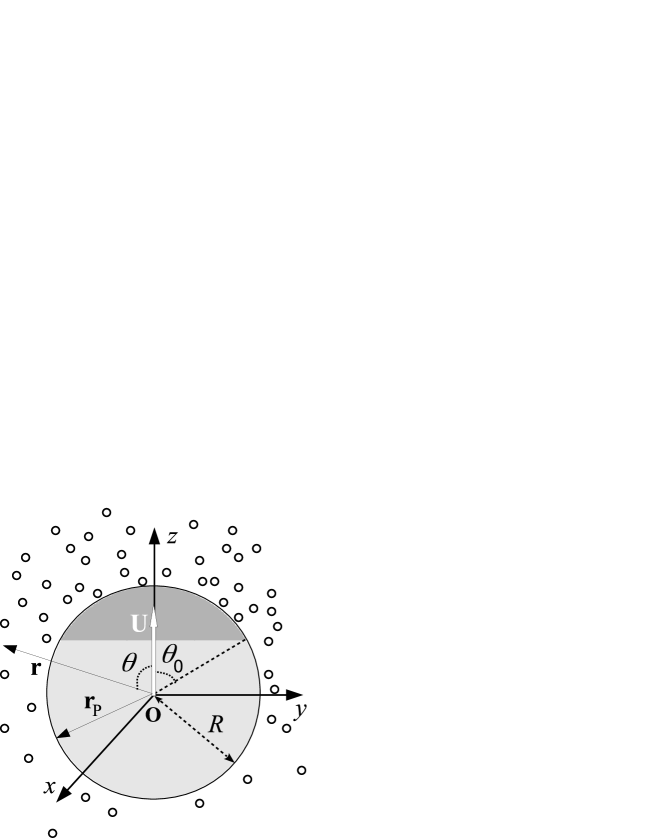
Figure 1: Schematic illustration of a chemically active spherical particle of radius $R$ immersed in an unbounded solution and moving with velocity $\mathbf{U}$ (white thick arrow). The two parts of the surface are spherical caps (dark gray and light gray areas, respectively) delimited by the latitudinal circle with polar angle $\theta_{0}$, and have different properties in terms of “chemical activity”. For instance, they can release or annihilate a solute molecule (small white circles) which diffuses in the surrounding solution, or they are chemically inert (i.e., neither releasing nor annihilating solute). Due to the distinct “chemical activity” of the two parts, a gradient in the solute density around the particle builds up (schematically indicated by the non-uniform distribution of the small white circles). The origin $O$ of the fixed (laboratory) system of coordinates is chosen such that it coincides with the instantaneous position of the center of the particle, and the $Oz$ axis is aligned with the axis of symmetry; $r$, $\theta$, and $\phi$ (not shown) denote the spherical coordinates defined in the usual way in the $Oxyz$ frame of reference; $\mathbf{r}_{P}$ is a point on the surface of the particle.

The simplest realization of sources and sinks is the so-called “constant-flux” boundary condition Golestanian et al. (2007); Brady (2011), i.e., at each point $\mathbf{r}_{P}$ at the surface of the particle the normal component of the solute current takes a prescribed, time-independent value given by ${\cal K}(\mathbf{r}_{P}):=Qf(\mathbf{r}_{P})$ (with units m${}^{-2}\times$ s^-1), where $Q>0$ is a prefactor which takes care of the dimensionality so that $f(\mathbf{r}_{P})$ is dimensionless. The latter will be referred to as the “activity function” and accounts for the sign of ${\cal K}(\mathbf{r}_{P})$ corresponding to “production” ($f>0$) or “annihilation” ($f<0$) of solute at $\mathbf{r}_{P}$. The more complex case of a reaction with first order kinetics, i.e., ${\cal K}(\mathbf{r}_{P})$ being proportional to the local density of a “fuel” species at $\mathbf{r}_{P}$, will be considered separately in, c.f., Sec. IV.

The motion of the particle and the diffusion of the molecular solute are assumed to be such that the Péclet number of the solute and the Reynolds number of the flow are very small, such that the number density of the solute relaxes towards the steady state distribution $c(\mathbf{r})$ much faster than the characteristic time scale of the motion of the particle (e.g., the time needed for the particle to pass a distance equal to its radius). The interaction of the solute molecules (in excess to the one of a solvent molecule de Groot and Mazur (1962); Jülicher and Prost (2009)) with the surface of the particle is encoded into a phoretic mobility coefficient $b(\mathbf{r}_{P}):=b_{0}g(\mathbf{r}_{P})$ (with the units m⁵/s), such that $g(\mathbf{r}_{P})$ is dimensionless and $b_{0}>0$ is a characteristic value (e.g., $b_{0}=(4\pi R^{2})^{-1}\int d^{2}\mathbf{r}_{P}|b(\mathbf{r}_{P})|$). The mobility coefficient describes the phoretic slip boundary condition Anderson (1989); Derjaguin et al. (1966),

$$\mathbf{u}_{s}(\mathbf{r}_{P})=-b_{0}g(\mathbf{r}_{P})\nabla_{||}c(\mathbf{r}_{P})\,,$$ (1)

for the hydrodynamic field $\mathbf{u}(\mathbf{r})$ of the surrounding solution. The phoretic mobility coefficient can be either positive or negative, depending on the attractive or repulsive character of the excess interaction of the solute with the surface. The sign of $b(\mathbf{r}_{P})$ will be accounted for by $g(\mathbf{r}_{P})$. Typical experimental realizations Paxton et al. (2004); Howse et al. (2007); Buttinoni et al. (2013); Lozano et al. (2016) are such that the surface (or the whole volume) of the particle consists of two parts composed of different materials but preserving axial symmetry. Accordingly, the surface of the model particle is divided into two spherical caps (the poles of which define the symmetry axis) corresponding to an opening polar angle $\theta_{0}$ (see Fig. 1). The activity function $f$ as well as, in general, the phoretic mobility $g$ differ over the two caps.

The translational and angular velocities of the particle follow from the requirement of zero net force and torque on the particle, consistent with the case of overdamped motion.

II.2 Active particle in an unbounded fluid

The dynamics of this model particle is governed by boundary-value problems for the chemical and hydrodynamic fields $c(\mathbf{r})$ and $\mathbf{u}(\mathbf{r})$, respectively, and by the force balance on the particle. Accordingly, in an unbounded, quiescent fluid, one has:
• Laplace equation for $c(\mathbf{r})$:

$$\nabla^{2}c(\mathbf{r})=0\,,$$ (2a)

with the boundary conditions (BCs)

$$-D\left.\left[\mathbf{n}\cdot\nabla c(\mathbf{r})\right]\right|_{\mathbf{r}=\mathbf{r}_{P}}=Qf(\mathbf{r}_{P})\,,$$ (2b)

where $$D$$ is the diffusion constant of the solute molecules, and

$$c(|\mathbf{r}|\to\infty)\to c_{\infty}\,.$$ (2c)

• incompressible Stokes equations for $\mathbf{u}(\mathbf{r})$:

$$\nabla\cdot\hat{\bm{\sigma}}=0\,,~{}~{}~{}~{}\nabla\cdot\mathbf{u}(\mathbf{r})=0\,,$$ (3a)

with the BCs

$$\mathbf{u}(\mathbf{r}_{P})=\mathbf{U}+\mathbf{u}_{s}(\mathbf{r}_{P})\,,$$ (3b)

$$\mathbf{u}(|\mathbf{r}|\to\infty)=0\,.$$ (3c)

In these equations, $\mathbf{u}_{s}(\mathbf{r}_{P})$ is given by Eq. (1),

$$\hat{\bm{\sigma}}:=-p\hat{\mathbf{I}}+\mu\left[\nabla\mathbf{u}+\left(\nabla\mathbf{u}\right)^{T}\right]\,$$ (4)

denotes the stress tensor (for a Newtonian fluid of viscosity $\mu$) with the pressure $p(\mathbf{r})$. $()^{T}$ indicates a transposed quantity; we use the convention that in the absence of an explicitly indicated operation two adjacent vectors (or vector operators) denote the tensor (dyadic) product.

• vanishing net force on the particle:

$$\mathbf{F}_{ext}+\int\limits_{|\mathbf{r}|=R}dS\,\hat{\bm{\sigma}}\cdot\mathbf{n}=0\,,$$ (5)

where $\mathbf{F}_{ext}$ denotes the external force on the particle.

In the following, we set $c_{\infty}=0$ without loss of generality. This amounts to introducing $c(\mathbf{r})\rightarrow\tilde{c}(\mathbf{r})=c(\mathbf{r})-c_{\infty}$ as the deviation from the “bulk” value $c_{\infty}$, which leaves Eqs. (1) and (2) unchanged. The model is therefore completely specified by providing the geometrical parameter $\theta_{0}$, the activity function $f(\theta)$, the phoretic mobility function $g(\theta)$, and the external forces acting on the spherical particle.

Before proceeding with the formal solution of Eqs. (1)-(5), dimensional analysis allows one to introduce the following quantities:
(i) from Eq. (2b), a characteristic number density

$$C_{0}:=\frac{QR}{D}\,;$$ (6a)

(ii) from Eqs. (1) and (6a), a characteristic velocity

$$U_{0}:=\frac{b_{0}C_{0}}{R}=\frac{Qb_{0}}{D}\,;$$ (6b)

(iii) and, from Eqs. (4) and (5), a characteristic force

$$F_{0}:=6\pi\mu RU_{0}\,,$$ (6c)

respectively. These provide the scales for the corresponding dimensional quantities.

II.3 Squirmer representation

By expanding $f(\theta)$ in terms of Legendre polynomials,

$$f(\theta)=\sum\limits_{n\geq 0}f_{n}P_{n}(\cos\theta)\,,$$ (7a)

where

$$f_{n}=(n+1/2)\int\limits_{0}^{\pi}d\theta\,\sin\theta\,f(\theta)P_{n}(\cos\theta)\,,$$ (7b)

the solution of the diffusion problem (Eqs. (2)(a)-(c)) can be expressed in terms of a multipole expansion Golestanian et al. (2007):

$$\frac{c(r,\theta)}{C_{0}}=\sum\limits_{n\geq 0}\frac{f_{n}}{n+1}\left(\frac{R}{r}\right)^{n+1}P_{n}(\cos\theta)\,.$$ (8)

The individual terms allow for clear physical interpretations: the first one (monopole) corresponds to a source or sink (net release or annihilation), the second one corresponds to a dipole (fore-aft asymmetry in release or annihilation), etc. Combining Eqs. (8), (1), and (61), and defining Lighthill (1952); Blake (1971)

$$V_{n}(\cos\theta)=\frac{2}{n(n+1)}P_{n}^{1}(\cos\theta)\,,$$ (9)

where $P_{n}^{1}(\cos\theta)$ denotes the associated Legendre function of degree $n$ and order 1 Abramowitz and Stegun (1972), renders the phoretic slip Bickel et al. (2013); Michelin and Lauga (2014); Ibrahim and Liverpool (2016)

$$\frac{\mathbf{u}_{s}}{U_{0}} = -\left[g(\theta)\sum\limits_{n\geq 1}\frac{f_{n}}{n+1}P_{n}^{1}(\cos\theta)\right]\mathbf{e}_{\theta}$$ (10)

$$:= \left(\sum\limits_{n\geq 1}B_{n}V_{n}(\cos\theta)\right)\mathbf{e}_{\theta}\,,$$

with

$$B_{n}=-\left(n+\frac{1}{2}\right)\sum\limits_{k\geq 1}\frac{f_{k}}{k+1}{\cal I}_{n,k}\,,$$ (11)

and

$${\cal I}_{n,k}:=\dfrac{1}{2}\int\limits_{0}^{\pi}d\theta\,\sin\theta\,g(\theta)P_{k}^{1}(\cos\theta)P_{n}^{1}(\cos\theta)\,.$$ (12)

Note that, with the exception of $f_{0}$, all coefficients $f_{k}$ in the expansion of the activity function contribute to each of the coefficients $B_{n}$ with weights ${\cal I}_{n,k}$ determined by the variation of the phoretic mobility encoded in $g(\theta)$.

As discussed in Refs. Bickel et al. (2013); Michelin and Lauga (2014); Ibrahim and Liverpool (2016) the hydrodynamic problem defined by Eq. (3), together with the expression for the phoretic slip (Eq. (10)) and the force-free condition (Eq. (5) with $\mathbf{F}_{ext}=0$) is mathematically identical to a “squirmer” model Blake (1971); Lighthill (1952). For reasons given below, it is advantageous to explicitly account for an external force $\mathbf{F}_{ext}=F\mathbf{e}_{z}$, which preserves the axial symmetry of the system.

Following standard procedure, by using the general results derived by Brenner Happel and Brenner (1973) for the flow around a sphere and the corresponding hydrodynamic force exerted on the sphere, we arrive at the following expressions for the flow field $\mathbf{u}(r,\theta)=u_{r}(r,\theta)\mathbf{e}_{r}+u_{\theta}(r,\theta)\mathbf{e}_{\theta}$ in the fixed laboratory frame:

$$\frac{u_{r}(r,\theta)}{U_{0}}=\frac{1}{2}\left[3\left(\frac{R}{r}\right)-\left(\frac{R}{r}\right)^{3}\right]\left(\frac{F}{F_{0}}\right)P_{1}(\cos\theta)\hskip 28.45274pt$$

$$\hskip 14.22636pt-\frac{2}{3}B_{1}\left(\frac{R}{r}\right)^{3}P_{1}(\cos\theta)$$

$$\hskip 14.22636pt+\sum\limits_{n\geq 2}\left[\left(\frac{R}{r}\right)^{n}-\left(\frac{R}{r}\right)^{n+2}\right]B_{n}P_{n}(\cos\theta)\,,$$

$$\frac{u_{\theta}(r,\theta)}{U_{0}}=\frac{1}{4}\left[-3\left(\frac{R}{r}\right)+\left(\frac{R}{r}\right)^{3}\right]\left(\frac{F}{F_{0}}\right)V_{1}(\cos\theta)$$

$$\hskip 14.22636pt+\frac{1}{3}B_{1}\left(\frac{R}{r}\right)^{3}V_{1}(\cos\theta)$$ (13b)

$$\hskip 14.22636pt-\frac{1}{2}\sum\limits_{n\geq 2}\left[(n-2)\left(\frac{R}{r}\right)^{n}-n\left(\frac{R}{r}\right)^{n+2}\right]B_{n}V_{n}(\cos\theta)\,.$$

The velocity $U:=\mathbf{U}\cdot\mathbf{e}_{z}$ of the particle is given by

$$\frac{U}{U_{0}}=\frac{F}{F_{0}}-\frac{2}{3}B_{1}\,.$$ (14)

(If needed, the flow field $\mathbf{u}^{C}(r,\theta)$, in a coordinate system aligned with $Oxyz$ and co-moving with the particle, is straightforwardly obtained as $\mathbf{u}^{C}(\mathbf{r})=\mathbf{u}(\mathbf{r})-\mathbf{U}$.)

Equation (13) identifies the contributions to the flow due to the external force (see the first line in Eqs. (13)(a) and (b)) and due to the phoretic slip – or self-motility – (i.e., the remaining terms). This reflects the linearity of the Stokes equations. Similarly, the expression for the velocity of the particle (Eq. (14)) reflects a contribution due to the external force (i.e., the first term on the right hand side (RHS)) and one due to self-propulsion. It is well established that the latter depends only on the first “squirmer mode” $B_{1}$ Lighthill (1952). There are two set-ups of particular interest (see also Ref. Bickel et al. (2013)): (a) a particle moving in the absence of external forces ($F=0$, force free (f)), with velocity $U=U^{(f)}$, and (b) a “stalling” (st) configuration, i.e., an active particle which is immobilized ($U=0$) due to an external force $F=F_{st}$ acting along the symmetry axis. In the first case, with $F=0$, Eq. (14) renders

$$U^{(f)}/U_{0}=-\frac{2}{3}B_{1}\,.$$ (15)

In the second case, with $U=0$, Eq. (14) renders

$$F_{st}/F_{0}=\frac{2}{3}B_{1}\,.$$ (16)

By combining the two relations, one finds Bickel et al. (2013); Oshanin et al. (2017)

$$F_{st}=-6\pi\mu RU^{(f)}\,,$$ (17)

which is a deceptively simple expression, in particular in view of its exact resemblance to the Stokes formula for a dragged spherical particle.

These results are relevant for experimental studies involving active particles. For example, it is very difficult to measure directly, by three-dimensional tracking a moving active particle Campbell and Ebbens (2013); Ebbens et al. (2014), the velocity $U^{(f)}$ of force-free motion in an unbounded fluid. (See also the measurements of the flow around a swimming micro-organism reported in Ref. Drescher et al. (2010).) On the other hand, if it is possible to realize a stall-force experiment by trapping an active particle far away from boundaries while minimally interfering with the mechanism of activity, i.e., without affecting the coefficient $B_{1}$, Eq. (17) provides the value $U^{(f)}$ from the measured stall force; the set-up in Ref. Ma et al. (2015) could provide such an example.

III Solute distribution and flow around active particles with constant-flux activity in unbounded space

We apply the results derived in the previous section in order to study how the choice of a constant-flux activity function, as well as variations in the phoretic mobility over the surface of the particle, influence the structure of the flow around such model active particles suspended in an unbounded fluid. Three model activities, which lend themselves for experimental realizations of active particles Golestanian et al. (2007); Howse et al. (2007); Ibrahim and Liverpool (2016); Moran and Posner (2016), will be considered: (i) $f^{(pi)}(\theta)$ describing a spatially uniform production of solute over one part of the surface, the other part being chemically inert; (ii) $f^{(pa)}(\theta)$ describing a uniform production of solute over one part of the surface and uniform annihilation (in general at a different rate) of the solute over the other part, such that there is no net production of solute by the particle; and (iii) $f^{(vi)}(\theta)$ describing a spatially varying production of solute over one part of the surface (presumably reflecting a certain systematic dependence of catalytic properties on the thickness of the coating for very thin films of catalysts Campbell and Ebbens (2013)), the other part being chemically inert. We shall discuss separately the case in which the phoretic mobility is position independent, focusing on the influence of $\theta_{0}$ on the resulting flow, and the case of a position dependent phoretic mobility which takes distinct values on the two parts of the surface. In the latter case, for which closed-form formulas cannot be derived, we restrict the discussion to the case of Janus colloids, i.e., $\theta_{0}=\pi/2$ (which experimentally is the most common case).

We employ the terminology of squirmers in order to discuss the force-free far-field flow of the corresponding model active particle. For a motile, force-free particle (i.e., $B_{1}\neq 0$), the second squirming mode $B_{2}$, which is related to the magnitude of the flow due to a stresslet Lighthill (1952); Blake (1971); Ishimoto and Gaffney (2013), provides that contribution to the flow with the slowest decay $\sim r^{-2}$ (see Eq. (13)). Therefore, the parameter $S:=-(B_{2}/|B_{1}|)$ (which we shall denote as “squirmer parameter”) has been used in the studies of squirmers in order to distinguish between pusher ($S<0$), puller ($S>0$), and neutral ($B_{2}=0$) squirmers. If $B_{2}=0$, the slowest decaying contribution to the flow is the one proportional to $r^{-3}$, which is the flow due to either a source-dipole or a force quadrupole Ishimoto and Gaffney (2013); Michelin and Lauga (2014). The squirming modes contributing to it are $B_{1}$ and $B_{3}$. For the models studied here, it does not occur that both coefficients $B_{2}$ and $B_{3}$ are vanishing simultaneously. Therefore the dependences of $S:=-(B_{2}/|B_{1}|)$ and $S^{\prime}=(B_{3}/B_{1})$ on the parameters of the model suffice to characterize the far-field hydrodynamic flow.

III.1 Position independent phoretic mobility $b(\mathbf{r}_{P})$

We chose $g(\theta)=-1$, which corresponds to a repulsive effective interaction between solute molecules and the surface of the particle. (The case $g(\theta)=+1$ can be obtained from the results presented here by simply changing the sign of the velocities for both the particle and the flow.) In this case, the weights ${\cal I}_{n,k}$ (Eq. (12)) take the simple form (see also Eq. (63))

$${\cal I}_{n,k}=-\frac{n(n+1)}{2n+1}\delta_{n,k}\,,$$ (18)

and each of the coefficients $B_{n}$ depends solely on the corresponding coefficient $f_{n}$ with the same index $n$:

$$B_{n}=\frac{nf_{n}}{2}\,.$$ (19)

As discussed in Ref. Golestanian et al. (2007), the straightforward implication of Eqs. (15) and (19) is that a spherical particle with uniform properties in terms of chemical activity – i.e., only the amplitude $f_{0}$ is nonzero – can neither exhibit self-motility (for which $U^{(f)}\neq 0$) nor induce flow in an unbounded fluid because in this case all coefficients $B_{n}$ vanish.

Figure 2: (a) The velocity $U^{(f)}$ of a force free particle as a function of the opening angle $\theta_{0}$ for three model activities (see the main text) and for a position-independent, negative phoretic mobility. The curve for $(vi)$ ends at $\theta_{0}=\pi/2$ because that model is defined for $\theta_{0}\leq\pi/2$ (see Eq. (29) in the main text). (b), (c) The squirmer parameters $S=-(B_{2}/B_{1})$ (note that $B_{1}>0$, panel (a)) and $S^{\prime}=B_{3}/B_{1}$ as functions of $\theta_{0}$ for the model activities (see the main text) $(pa)$ and $(pi)$ (panel (b)) and $(vi)$ (panel (c)) for a position-independent, negative phoretic mobility. The open interval marks in (b) and (c) remind that $S$ and $S^{\prime}$ are not defined at $\theta_{0}=0$, where $B_{1}$ vanishes, but their limits as $\theta_{0}\to 0$ exist.

III.1.1 Particle with position-independent activity over a spherical cap and being inert over the rest of the surface

The activity function corresponding to this case is given by

$$f^{(pi)}(\theta)=\begin{cases}1,~{}&0\leq\theta<\theta_{0}\,,\\ 0,~{}&\theta_{0}<\theta\leq\pi\,,\end{cases}$$ (20)

with $0<\theta_{0}<\pi$. The cases of a completely inert ($\theta_{0}=0$) or an entirely active ($\theta_{0}=\pi$) particle, which – owing to the spherical symmetry – are not motile in an unbounded fluid, are excluded from the discussion here. The corresponding amplitudes $f_{n}$ are (see Eq. (64))

$$f_{n}^{(pi)}(\theta_{0})=\begin{cases}\dfrac{1}{2}(1-\cos\theta_{0})>0\,,&n=0\,,\\ -\dfrac{n+1/2}{n(n+1)}\,\sin\theta_{0}P_{n}^{1}(\cos\theta_{0})\,,&n\geq 1\,,\end{cases}$$ (21)

and the velocity corresponding to force-free motion is given by

$$\frac{U^{(f)}_{pi}}{U_{0}}=-\frac{\sin\theta_{0}^{2}}{4}<0\,,$$ (22)

i.e., as expected Golestanian et al. (2007), the motion is in the negative $z$ direction (away from the active cap), irrespective of the value of $\theta_{0}$ (see also Fig. 2(a)). The dependence of the velocity $U^{(f)}_{pi}$ on $\theta_{0}$, shown by the solid line in Fig. 2(a), exhibits the expected symmetry with respect to $\theta_{0}=\pi/2$ Golestanian et al. (2007); Popescu et al. (2010).

Since $B_{1}(\theta_{0})\geq 0$, the parameters $S$ and $S^{\prime}$ corresponding to this model activity function are given by

$$S_{pi}:=-\frac{B_{2}}{B_{1}}=-\frac{10}{3}\cos\theta_{0}\,,$$ (23a)

and

$$S^{\prime}_{pi}:=\frac{B_{3}}{B_{1}}=\frac{7}{4}\left(5\cos^{2}\theta_{0}-1\right)\,,$$ (23b)

and are shown in Fig. 2(b). One notices that $S_{pi}(\theta_{0})$ is negative for $\theta_{0}<\pi/2$ and that it changes sign at $\theta_{0}=\pi/2$. (At that point, $S^{\prime}_{pi}$ is non-zero and negative (see Fig. 2(b)), in agreement with the observation that for the models we consider the two coefficients do not vanish simultaneously.) Therefore, the far-field flows in this model correspond to those of a pusher ($\theta_{0}<\pi/2$), neutral ($\theta_{0}=\pi/2$), and puller ($\theta_{0}>\pi/2$), respectively (see also, c.f., Fig. 3). Thus by varying $\theta_{0}$ this model can exhibit the whole spectrum (puller, pusher, neutral) of squirmer behaviors. In view of the results reported in Ref. Delfau et al. (2016), this could be advantageously exploited in, e.g., studies of the collective behavior of chemically active particles.

This model has been extensively studied (see, e.g., Refs. Golestanian et al. (2007); Popescu et al. (2010); Michelin and Lauga (2014); de Graaf et al. (2015); Moran and Posner (2016); Reigh and R. (2015)) and representative plots of the solute distribution (see, e.g., Ref. Michelin and Lauga (2014)), the phoretic slip distribution, and the flow field (see, e.g., Refs. Bickel et al. (2013); Reigh and R. (2015); de Graaf et al. (2015); Eskandari (2016)) corresponding to this model can be found in the literature. Furthermore, it turns out that the phoretic slip distribution and the hydrodynamic flow exhibit patterns similar to the ones corresponding to model $(pa)$ (see next subsection), and therefore they will be discussed there.

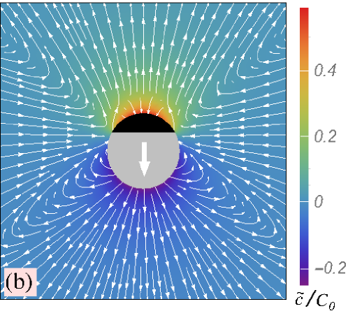
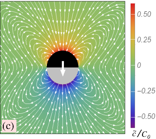
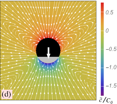
Figure 3: (a) Phoretic slip $u_{s}:=\mathbf{u}_{s}\cdot\mathbf{e}_{\theta}$ for model $(pa)$ as a function of the angular position $\theta$ [Eq. (10), truncated at the first 300 terms] for opening angles $\theta_{0}=\pi/3$, $\pi/2$, and $2\pi/3$, respectively. (b)-(d) The force-free flow field in the laboratory system (lines) (Eq. (13)) and the distribution of solute (color coded) relative to the bulk density (Eq. (8)) for model $(pa)$ and opening angles $\theta_{0}=\pi/3$, $\pi/2$, and $2\pi/3$, respectively. For both the density and the flow the series are truncated at the first 50 terms. The thick white arrows show the direction of the motion of the particle. In (a)-(d) the phoretic mobility is position independent and negative.

III.1.2 Particle with position-independent production or annihilation activity, respectively, over the two spherical caps

The activity function corresponding to this case is given by

$$f^{(pa)}(\theta)=\begin{cases}1,~{}&0\leq\theta<\theta_{0}\,,\\ q,~{}&\theta_{0}<\theta\leq\pi\,.\end{cases}$$ (24)

By imposing that there is no net production or annihilation of solute, the value of the parameter $q$ is fixed to

$$q=-\frac{1-\cos\theta_{0}}{1+\cos\theta_{0}}<0\,.$$ (25)

The parameter $0<\theta_{0}<\pi$, i.e., the cases of in which the whole surface is either producing or annihilating, respectively, are excluded from the discussion here. (Moreover, the limit $\theta_{0}\to\pi$ is unphysical because in that case there is a point-like sink with a diverging rate of annihilation.) The corresponding amplitudes $f_{n}$ are given by (see Eq. (64))

$$f_{n}^{(pa)}(\theta_{0})=\begin{cases}0\,,&n=0\,,\\ -\dfrac{2n+1}{n(n+1)}\dfrac{P_{n}^{1}(\cos\theta_{0})}{1+\cos\theta_{0}}\,,&n\geq 1\,.\end{cases}$$ (26)

As expected, due to the requirement that there is no net production or annihilation, the amplitude $f_{0}$ of the monopole term vanishes. For three values of $\theta_{0}$, the number density $\tilde{c}(\mathbf{r})$ of solute in excess of the bulk density is shown as color code in Figs. 3 (b)-(d). In all cases there is a region of excess density (red color) around the cap which releases solute and a depletion region (deep blue up to violet color) around the cap which annihilates solute. The size of these regions as well as the magnitude of the excess or the depletion (see the range of the color bars at the right of the corresponding panels) increases upon increasing the size of the release area (i.e., upon increasing $\theta_{0}$), while the dipolar structure of the solute distribution becomes more pronounced.

The velocity corresponding to force-free motion is given by

$$\frac{U^{(f)}_{pa}}{U_{0}}=-\frac{1}{2}\tan\left(\frac{\theta_{0}}{2}\right)<0\,,$$ (27)

i.e., as for the model $(pi)$, also in this case the motion is in the direction of negative $z$ (i.e., away from the active cap), irrespective of the value of $\theta_{0}$ (see also Fig. 2(a)). However, the dependence on $\theta_{0}$ is different due to the change in the activity over the lower cap: the gradients of the solute number density along the surface are enhanced (see Fig. 3), and, as a consequence, in this model the magnitude of the force-free velocity is larger than that in the model $(pi)$ and exhibits a monotonic increase with $\theta_{0}$. As $\theta_{0}$ approaches $\pi$, the absolute value of the peak in the phoretic slip distribution increases and diverges for $\theta_{0}\to\pi$. As discussed above, in that limit the latter is an unphysical feature due to the model being ill-defined with a diverging rate of annihilation.

By comparing Eqs. (26) and (21), one concludes that for a given $\theta_{0}$ the parameters $S_{pa}$ and $S^{\prime}_{pa}$ (and, in general, all ratios $B_{n}/B_{1}$, $n\geq 2$) take the same values as those corresponding to the model $(pi)$ analyzed in the previous subsection, i.e.,

$$S_{pa}=S_{pi}\,,~{}~{}S^{\prime}_{pa}=S^{\prime}_{pi}\,.$$ (28)

Therefore, as noticed above, the flow field and the phoretic slip distribution have the same characteristics and appearances as the ones corresponding to the case $(pi)$; they differ only in magnitude by a $\theta_{0}$-dependent velocity scale factor $B_{1}^{(pi)}/B_{1}^{(pa)}=\sin\theta_{0}\cos^{2}(\theta_{0}/2)$. Accordingly, one can conclude that the two models, although physically different with respect to the mechanism and the character of their chemical activity, exhibit, up to a velocity scale factor, similar hydrodynamic fields associated with their motion in an unbounded fluid.

As shown in Fig. 3(a), the phoretic slip over the surface of the particle is negative everywhere (i.e., it points into the direction of $-\mathbf{e}_{\theta}$, and thus towards the region with higher density of solute) Accordingly, the particle moves into the opposite direction (see the thick white arrows), in line with the sign in Eq. (27). (We note that here and below the series representation of the phoretic slip in Eq. (10) has been truncated at the first 300 terms.) The magnitude of the phoretic slip varies non-monotonically with the angular position $\theta$ along the surface and, as discussed in, e.g., Ref. de Graaf et al. (2015), it has a sharply peaked maximum (but, despite of the appearance, there is neither a divergence nor a cusp) at $\theta_{0}$, where the discontinuity in the activity function is located.

The flow fields in the laboratory system are shown in Figs. 3(b)-(d) for three values of the parameter $\theta_{0}$ selected such that, according to the discussion above and in the previous subsection of the squirmer parameter $S$, the far-field behavior corresponds to a pusher ($\theta_{0}<\pi/2$), a neutral ($\theta_{0}=\pi/2$), and a puller ($\theta_{0}>\pi/2$) squirmer, respectively. (Note that these values correlate with the phoretic slip distribution (Fig. 3(a)) being significantly peaked at the hemisphere with the active pole, at the equator, and at the hemisphere with the inert pole, respectively.) The presence of a stagnation point for $\theta_{0}<\pi/2$ (Fig. 3(b)) and $\theta_{0}>\pi/2$ (Fig. 3(d)), respectively, and its location behind or ahead of the particle, respectively, are indeed consistent with the pusher and puller characteristics. The clear fore-aft symmetry of the streamlines in Fig. 3(c), for which $\theta_{0}=\pi/2$ and thus $S=0$, is expected for a neutral squirmer. In all three cases there are strong deviations of the shape of the streamlines from the expected far-field ones. In the case of the neutral squirmer, the formation of a “saddle”- or “butterfly”-like feature at $\theta\simeq\pi/2$ is particularly noteworthy. This signals that for $r/R\simeq 4$ the squirming modes with $n\geq 3$ still make significant contributions to the flow around the active particle.

Finally, we note that $\tilde{c}(\mathbf{r})$, as shown in Figs. 3(b)-(d), underscores that in order for the model $(pa)$ to be well defined, i.e., the solute number density $c(\mathbf{r})$ to be non-negative everywhere, the background number density $c_{\infty}$ must be sufficiently large. This is a result of the assumption that the annihilation reaction has a constant rate independent of, rather than being proportional to, the local density of solute molecules. Although this assumption reduces the significance of the results for experimental studies, it has the merit of providing the means for straightforwardly building a conceptually clear example that two different models of activity can lead to effective squirmers which exhibit identical behaviors (in the sense of identical coefficients $B_{n}$ for $n\geq 2$). Furthermore, the generalization to activity functions corresponding to reactions with first-order kinetics will be discussed in Sec. IV.

III.1.3 Particle with position-dependent production over a spherical cap and being inert over the rest of the surface

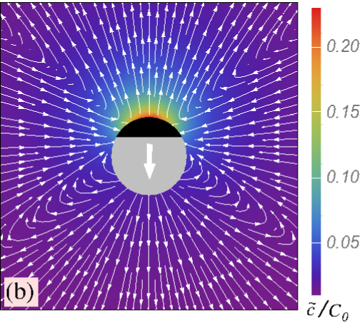
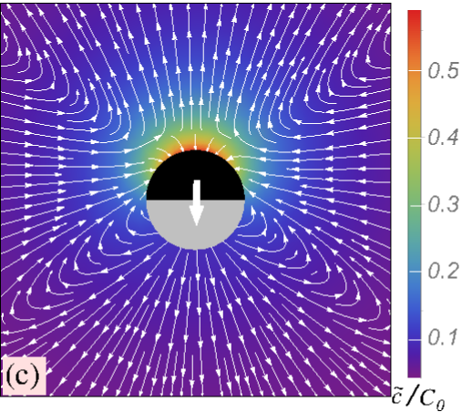
Figure 4: (a) Phoretic slip for model $(vi)$ as a function of position $\theta$ [Eq. (10), truncated at the first 300 terms] for opening angles $\theta_{0}=\pi/3$ and $\pi/2$, respectively. (b), (c) The force-free flow field in the laboratory system (lines, Eqs. (13)), and the distribution of solute (color coded) relative to the bulk density (Eq. (8)) for model $(vi)$ and opening angles $\theta_{0}=\pi/3$ and $\pi/2$, respectively. For both density and flow the series are truncated at the first 50 terms. The thick white arrows show the direction of the motion for the particle. In (a)-(c) the phoretic mobility is position independent and negative.

The activity function corresponding to this case is chosen to be of the form

$$f^{(vi)}(\theta)=\begin{cases}\cos\theta-\cos\theta_{0},~{}&0\leq\theta<\theta_{0}~{}(\leq\pi/2)\,,\\ 0,~{}&\theta_{0}\leq\theta\leq\pi\,.\end{cases}$$ (29)

This choice is motivated by Refs. Campbell and Ebbens (2013); Brown and Poon (2014), in which it is argued, based on experimental evidence, that there is a possible dependence of the activity on the thickness of the catalyst coating. This thickness varies on the surface of the sphere from a maximum at the pole towards a minimum (i.e., no catalyst) upon approaching the equator. For reasons of simplicity, the parameter $\theta_{0}$ is constrained to the typical range $0<\theta_{0}\leq\pi/2$ employed in experimental studies. The constant term $\cos\theta_{0}$ ensures that the activity function is continuous at $\theta_{0}$.

By using Eqs. (64) and (65), the corresponding amplitudes $f_{n}$ (see Eq. (7)) can be expressed as

$$f_{n}^{(vi)}(\omega_{0})=\left(n+\frac{1}{2}\right)\left(1-\omega_{0}^{2}\right)^{1/2}$$

$$\times \left[\frac{P_{1}(\omega_{0})P_{n}^{1}(\omega_{0})}{n(n+1)}-\frac{P_{n}(\omega_{0})P_{1}^{1}(\omega_{0})-P_{1}(\omega_{0})P_{n}^{1}(\omega_{0})}{2-n(n+1)}\right]\,,$$

where $\omega_{0}:=\cos(\theta_{0})$.

The velocity corresponding to force-free motion is given by

$$\frac{U^{(f)}_{vi}}{U_{0}}=-\frac{1}{12}\,\left[2+\cos\theta_{0}\left(\cos^{2}\theta_{0}-3\right)\right]\,.$$ (31)

For $0<\theta_{0}\leq\pi/2$ one has $U^{(f)}_{vi}/U_{0}<0$ (see Fig. 2(a)). As expected, the motion is in the negative $z$ direction (i.e., away from the active cap), which is consistent with the phoretic slip pointing towards the $-\mathbf{e}_{\theta}$ direction (see Fig. 4(a)). The smoothly decreasing production rate over the surface leads to smaller gradients in the solute number density and, accordingly, to visibly reduced velocities in comparison to those in the previous two models. This also leads to the removal of the sharp peaks, as observed in the other models, in the distribution of the phoretic slip around the surface of the particle (see Fig. 4(a)).

From Eq. (III.1.3) one obtains the parameters $S$ and $S^{\prime}$ as

$$S_{vi}:=-\frac{B_{2}}{|B_{1}|}=-\frac{5}{2}\,\dfrac{\sin^{4}\theta_{0}}{2+\cos\theta_{0}\left(\cos^{2}\theta_{0}-3\right)}$$ (32a)

and

$$S^{\prime}_{vi}:=\frac{B_{3}}{B_{1}}=\frac{21}{4}\,\dfrac{\cos\theta_{0}\,\sin^{4}\theta_{0}}{2+\cos\theta_{0}\left(\cos^{2}\theta_{0}-3\right)}\,,$$ (32b)

respectively. Their dependence on $\theta_{0}$ is shown in Fig. 2(c). As for the other models, $S_{vi}(\theta_{0})<0$ for $\theta_{0}<\pi/2$; but it remains negative also at $\theta_{0}=\pi/2$. Therefore, within the whole range of $\theta_{0}$ the far-field flows in this model correspond to those of a pusher. This is illustrated in Figs. 4(b)-(c), where we show the flows for $\theta_{0}=\pi/3$ (b) and $\theta_{0}=\pi/2$ (c).

III.2 Position dependent phoretic mobility $b(\mathbf{r}_{P})$

As noted in the beginning of Sec. III, if the phoretic mobility varies over the surface it is not possible, in general, to obtain simple expressions – such as, e.g., Eq. (19) – for the coefficients $B_{n}$. Therefore we continue the discussion of the model activity functions under additional constraints in order to reduce the number of free parameters. We shall focus on the case $\theta_{0}=\pi/2$, which is a typical value in experimental studies, and we shall consider only models with the phoretic mobility described by a piecewise constant function:

$$g(\theta)=\begin{cases}-1,&0\leq\theta<\theta_{0}=\pi/2,\\ -\gamma,&\pi/2=\theta_{0}<\theta\leq\pi.\end{cases}$$ (33)

This corresponds to a negative phoretic mobility $-b_{0}$ over the upper cap (see Fig. 1) and a different value, $-\gamma\,b_{0}$, over the lower cap. This choice is motivated by the typical realizations of such particles, in which the two parts of the particle consist of two distinct materials (such as the Au-Pt rods employed in the experiments reported in Ref. Paxton et al. (2004)); alternatively, a part of their surface is coated by a different material. This is, e.g., the case for the particles employed in Ref. Simmchen et al. (2016) for which one part is silica (inactive) while the other part is covered by Pt catalyst (active). We note that $\gamma=1$ corresponds to models with position independent phoretic mobility, as studied in the previous subsection.

With this choice for $g(\theta)$, the weights ${\cal I}_{n,k}$ (Eq. (12)) take the form

$${\cal I}_{n,k} = -\frac{1+(-1)^{n+k}\,\gamma}{2}\int\limits_{0}^{1}dxP_{n}^{1}(x)P_{k}^{1}(x)$$ (34)

$$=: -\frac{1+(-1)^{n+k}\,\gamma}{2}J_{n,k}\,,~{}~{}n,k\geq 1\,.$$

Although an insightful, closed form expression for the integrals $J_{n,k}$ defined above is not available, certain simplifications of the calculations below are possible by noticing that if $n+k$ is an even number one has

$$J_{n,k} := \int\limits_{0}^{1}dxP_{n}^{1}(x)P_{k}^{1}(x)=\frac{1}{2}\int\limits_{-1}^{1}dxP_{n}^{1}(x)P_{k}^{1}(x)$$ (35)

$$= \frac{n(n+1)}{2n+1}\delta_{n,k}\,,~{}~{}\mathrm{for}~{}n,k\geq 1\,,~{}n+k~{}\mathrm{even}.~{}~{}~{}$$

Furthermore, as discussed in the previous section, in the models $(pa)$ (production and annihilation) and $(pi)$ (production and inert) the coefficients $f_{n}$ with $n\geq 1$, and therefore the coefficients $B_{n}$, differ only by a constant factor independent of $n$ (e.g., for $\theta_{0}=\pi/2$, the coefficients $f^{(pi)}_{n}$ are twice as large as the coefficients $f^{(pa)}_{n}$). Consequently, the ensuing hydrodynamic flows they induce have the same structure and differ solely in terms of a velocity scale, irrespective of the specific dependence of the phoretic mobility on the position at the surface. Thus in the remaining part of this subsection we study only the models $(pa)$ and $(vi)$.

III.2.1 Production and annihilation (pa) activity function

In this case and for $\theta_{0}=\pi/2$ only the coefficients $f_{n}^{(pa)}$ with an odd index $n$ are nonzero (see Eq. (26)). Consequently, from Eqs. (11), (34), and (35) one concludes that for this model the coefficients $B_{n}$ are given by

$$B_{n}=\left[1+(-1)^{n+1}\gamma\right]\chi_{n}\,,~{}~{}n\geq 1\,,$$ (36)

where

$$\chi_{n}=\frac{1}{4}\times\begin{cases}nf_{n}^{(pa)}\,,&~{}n~{}\textrm{odd}\,,\\ (2n+1)\displaystyle{\sum\limits_{k~{}\mathrm{o}dd}}J_{n,k}\,\dfrac{f_{k}^{(pa)}}{k+1}\,,&~{}n~{}\textrm{even}\,.\end{cases}$$ (37)

Therefore, by combining Eqs. (15), (26), (36), and (37) one arrives at the following simple expression for the force-free velocity in an unbounded fluid:

$$\frac{U^{(f)}}{U_{0}}=-\frac{1+\gamma}{6}f_{1}^{(pa)}=-\frac{1+\gamma}{4}\,.$$ (38)

This expression shows that, as discussed in Ref. Golestanian et al. (2007), even if the phoretic mobility varies over the surface, i.e., $\gamma\neq 1$, a spatial variation in the activity, i.e., $f_{1}^{(pa)}\neq 0$, remains a necessary condition for self-motility ($U^{(f)}\neq 0$). One also finds that for $\gamma=-1$ (i.e., if the phoretic mobility over that hemisphere, where the solute is released, is equal in magnitude but opposite in sign to the one over the hemisphere where the solute is annihilated) the velocity vanishes. Nevertheless, the particle still induces a hydrodynamic flow. In the language of squirmers, this situation corresponds to a “shaker” ($S\to\pm\infty$). For $\gamma<-1$, the velocity reverses sign, and the force-free active particle moves in the positive $z$ direction, i.e., towards that cap where the solute is produced (see Fig. 5(a)).

Figure 5: (a) The velocity $U^{(f)}$ of a force-free spherical Janus particle ($\theta_{0}=\pi/2$) as a function of the ratio $\gamma$ of the phoretic mobilities over the two hemispheres, for the model activities (see the main text) $(pa)$ (dashed line) and $(vi)$ (dotted line). (b), (c) The squirmer parameters $S=-(B_{2}/|B_{1}|)$ and $S^{\prime}=B_{3}/B_{1}$ as functions of the ratio $\gamma$ for the model activities $(pa)$ (panel (b)) and $(vi)$ (panel (c)). In all three panels (a)-(c) the phoretic mobility over the upper hemisphere ($\theta<\pi/2$, see Fig. 1), where the solute is released into solution, is negative. The left and right open interval signs in panel (b) indicate that the function $S^{\prime}_{pa}$ is not defined at $\gamma=-1$ (where $B_{1}$ vanishes), but the left and right limits $S^{\prime}_{pa}(\gamma\to-1)$ do exist.

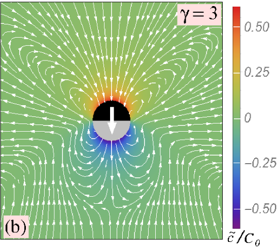
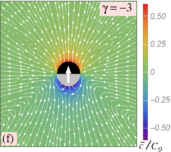
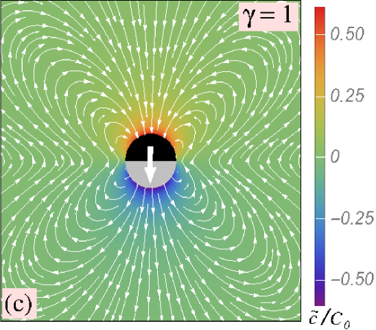
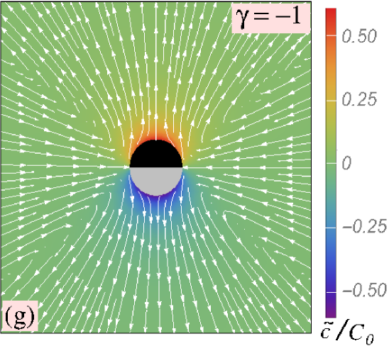
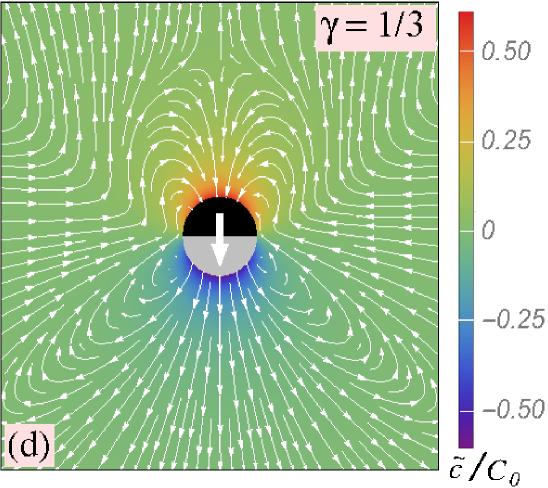
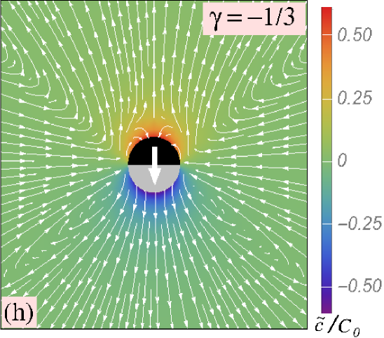
Figure 6: (a), (e): Phoretic slip as a function of position $\theta$ [Eq. (10), truncated at the first 300 terms] for model $(pa)$ with a binary-valued phoretic mobility (Eq. (33)) and for values $\gamma>0$ (panel (a)) and $\gamma<0$ (panel (e)). The open circles show the phoretic slip obtained by multiplying with a factor $\gamma=\pm 3$, respectively, the branch $\theta>\pi/2$ of the corresponding $(pa)$ result at $\theta_{0}=\pi/2$ from Sec. III.1. The solid curve ($\gamma=1$) in (a) corresponds to a particle with the same phoretic mobility $-b_{0}$ over the whole surface and thus reproduces (up to numerical accuracy, see the main text) the curve $\theta_{0}=\pi/2$ in Fig. 3(a). For $\theta<\pi/2$, in each panel all three curves coincide. Note that for $\gamma\neq 1$ there is a discontinuity at $\theta=\pi/2$ owing to the binary-valued phoretic mobility (see Eq. (33) and the main text). (b)-(d) and (f)-(h): The flow field in the laboratory system (lines, Eq. (13) and the number density of solute (color coded) relative to the bulk density (Eq. (8)) for model $(pa)$ with a binary-valued phoretic mobility function (Eq. (33)) and for values $\gamma>0$ (panels (b)-(d)) and $\gamma<0$ (panels (f)-(h)), respectively. For both the density and the flow the series are truncated at the first 50 terms. The thick white arrows show the direction of the motion of the particle. In all cases the phoretic mobility is negative over the hemisphere where the solute is released.

The mode $B_{2}$, which enters into the definition of the squirmer parameter $S$, cannot be determined analytically in closed form; on the other hand, Eqs. (36) and (37) do render an expression of closed form for the mode $B_{3}$. By numerically evaluating the coefficient $\chi_{2}$ in Eq. (37), we obtain $\chi_{2}\simeq-0.44$. For $n\leq 300$, the series entering in the definition of the coefficients $B_{n}$ have been evaluated by keeping the first $k\leq 200$ terms in Eq. (37); this ensured convergence of the truncation in all cases. With respect to the evaluation of the slip velocity over the surface of the particle, the discontinuity of the phoretic slip (due to the binary-valued phoretic mobility (Eq. (33))) at $\theta_{0}=\pi/2$ cannot be captured accurately by a truncated series representation (Eq. (10)) even if one keeps up to $n=300$ coefficients $B_{n}$. However, the result appears to be reasonably accurate, as shown in Figs. 6(a) and (e), except near the discontinuity at $\theta_{0}=\pi/2$, where the curves are still slightly noisy. A cross-check is provided by the observation that for the phoretic mobility defined in Eq. (33), the slip distribution can be obtained from the one at $\theta_{0}=\pi/2$ shown in Fig. 3(a) by leaving the branch $\theta<\pi/2$ unchanged while multiplying the branch $\theta>\pi/2$ with the factor $\gamma$. For $\gamma=\pm 3$, the result of this procedure is shown in Figs. 6(a) and (e) by symbols (circles); it compares very well with the results obtained from Eq. (10) (solid lines).

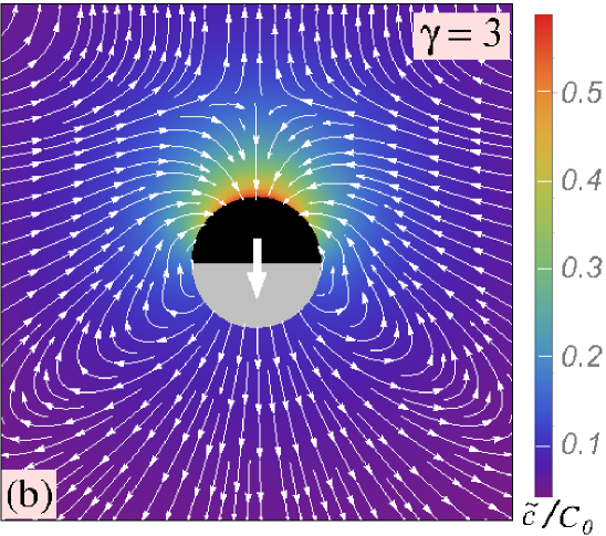
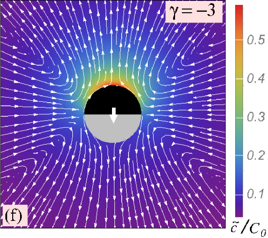
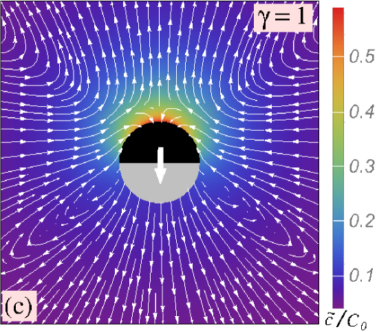
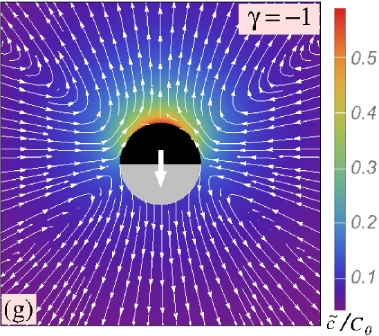
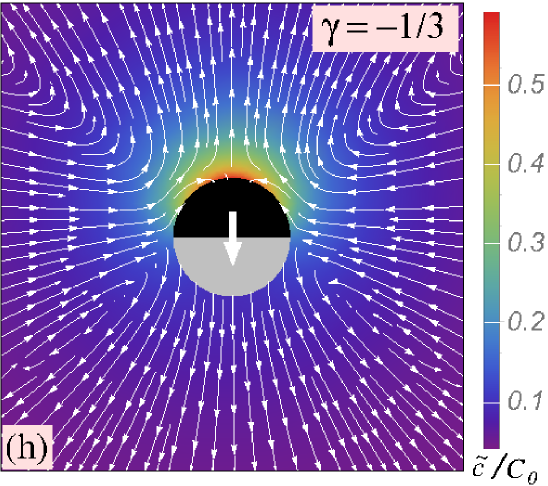
Figure 7: (a), (e): Phoretic slip as a function of position $\theta$ [Eq. (10), truncated at the first 300 terms] for model $(vi)$ with a binary-valued phoretic mobility (Eq. (33)) and for values $\gamma>0$ (panel (a)) and $\gamma<0$ (panel (e)). The open circles show the phoretic slip obtained by multiplying with a factor $\gamma=\pm 3$ the branch $\theta>\pi/2$ of the corresponding result for $(vi)$ at $\theta_{0}=\pi/2$ from Sec. III.1. For $\theta<\pi/2$, in each panel all three curves coincide. Note that for $\gamma\neq 1$ there is a discontinuity at $\theta=\pi/2$ owing to the binary-valued phoretic mobility (see Eq. (33) and the main text). (b)-(d) and (f)-(h): The flow field in the laboratory system (lines, Eqs. (13)) and the number density of solute (color coded) relative to the bulk density (Eq. (8)) for model $(vi)$ with a binary-valued phoretic mobility function (Eq. (33)) and for values $\gamma>0$ (panels (b)-(d)) and $\gamma<0$ (panels (f)-(h)), respectively. For both the density and the flow the series are truncated at the first 50 terms. The thick white arrows show the direction of the motion of the particle; the shorter arrow in panel (f) is a reminder that at $\gamma=-3$ the behavior is very similar to that of a shaker (which corresponds to $\gamma\simeq-3.4$). In all cases the phoretic mobility is negative over the hemisphere where the solute is released.

The parameters $S$ and $S^{\prime}$ are thus given by

$$S_{pa}:=-\frac{B_{2}}{|B_{1}|}\simeq 1.16\times\frac{\gamma-1}{|\gamma+1|}\,,\textrm{ for }\gamma\neq-1\,,$$ (39a)

$$S^{\prime}_{pa}:=B_{3}/B_{1}=-\frac{7}{4}\,,\textrm{ for }\gamma\neq-1\,;$$ (39b)

they are shown in Fig. 5(b). For $\gamma>1$ one has $S_{pa}>0$ and the far-field flow is that of a puller (Fig. 6(b), see the location of the stagnation point in front of the particle). For $\gamma<1$, $\gamma\neq-1$, $S_{pa}$ takes the opposite sign, $S_{pa}<0$, which is reflected by a far-field flow corresponding to a pusher (Figs. 6(d), (f), and (h)). For $\gamma=1$, one has $S_{pa}=0$ and the particle behaves as a neutral squirmer (Fig. 6(c)). For $\gamma\to-1$, for which the velocity vanishes, the squirmer parameter $S_{pa}$ diverges ($S_{pa}\to-\infty$) and, as mentioned above, the particle behaves as a shaker; the corresponding flow field is illustrated in Fig. 6(g)). The change in sign of $S_{pa}$ upon decreasing $\gamma$ occurs ahead of the change in sign of the velocity. Accordingly, in the range $-1<\gamma<1$ the particle maintains the motion away from the “producing” cap but changes its hydrodynamic signature from a puller (as it is for $\gamma>1$) to a pusher, which implies that the stagnation point is now located behind the particle. Finally, we note that, as can be read off from Eq. (39a), in the limit of a very large ratio of mobilities, i.e., $\gamma\to\pm\infty$, the squirmer parameter $S_{pa}$ attains the limiting values $S_{pa}\to\pm 1$.

III.2.2 Variable production and inert (vi) activity function

The analysis of model $(vi)$ proceeds along very similar lines. For $\theta_{0}=\pi/2$, all coefficients $f_{n}^{(vi)}$ of odd index $n$, with the exception of $f_{1}^{(vi)}$, vanish (see Eq. (26)). Consequently, Eqs. (11)-(35) render the coefficients

$$B_{n}=\left[1+(-1)^{n+1}\gamma\right]\xi_{n}+\left[1+(-1)^{n}\gamma\right]\nu_{n}\,,~{}n\geq 1\,,$$ (40)

where

$$\xi_{n}=\frac{n+1/2}{4}\,f_{1}^{(vi)}\,J_{n,1}$$ (41a)

and

$$\nu_{n}=\frac{1}{4}\times\begin{cases}nf_{n}^{(vi)}\,,&~{}n~{}\textrm{even}\,,\\ (2n+1)\displaystyle{\sum\limits_{k>0,~{}\mathrm{e}ven}}J_{n,k}\,\dfrac{f_{k}^{(vi)}}{k+1}\,,&~{}n~{}\textrm{odd}\,.\end{cases}$$ (41b)

Thus for this model the coefficients $B_{n}$ with $n$ odd have to be evaluated numerically by suitably truncating – typically after 200 terms – the series entering into the definition of $\nu_{n}$.

By combining Eqs. (15), (III.1.3), (40), and (41) one arrives at the following expression for the force-free velocity in an unbounded fluid:

$$\frac{U^{(f)}}{U_{0}}\simeq-\frac{2}{3}\left[0.07\,(1-\gamma)+\frac{1}{8}\,(1+\gamma)\right]\,;$$ (42)

this is shown as a dotted line in Fig. 5(a). This behavior is very similar to the one of model $(pa)$ discussed above: for $\gamma>\gamma_{c}\simeq-3.4$ the velocity is negative (i.e., the particle moves away from the active cap), while for $\gamma<\gamma_{c}$ the particle moves in the positive $z$ direction, i.e., towards the active cap. At $\gamma=\gamma_{c}$ the velocity vanishes and the hydrodynamic flow field induced by the particle resembles that of a shaker – very similar to the flow illustrated in Fig. 7(f) for $\gamma=-3$.

As with the model corresponding to Fig. 6, upon evaluating the slip velocity over the surface of the particle (Eq. (10)) the discontinuity (due to the bi-valued phoretic mobility (Eq. (33))) at $\theta_{0}=\pi/2$ cannot be captured accurately by a truncated series representation, even if keeping up to $n=300$ coefficients $B_{n}$. However, the result of such a truncation turns out to be reasonably accurate, as shown in Figs. 7(a) and (e), except near $\theta_{0}=\pi/2$, where some noise in the curves remains visible. Furthermore, as for the previously discussed model, the cross-check with the slip distribution obtained from the one in Fig. 4(a) at $\theta_{0}=\pi/2$ by multiplying the branch $\theta>\pi/2$ with the factor $\gamma$ (shown by open circles in Figs. 7(a) and (e) for $\gamma=\pm 3$) is satisfactory.

The parameters $S$ and $S^{\prime}$ are given by

$$S_{vi} := -\frac{B_{2}}{|B_{1}|}\simeq\frac{-0.4+0.08\,\gamma}{|0.2+0.06\,\gamma|}\,,\textrm{ for }\gamma\neq\gamma_{c}\,,$$

$$S^{\prime}_{vi} := B_{3}/B_{1}\simeq\,\frac{0.07\,(1-\gamma)}{0.2+0.06\,\gamma}\,,\textrm{ for }\gamma\neq\gamma_{c}\,;$$ (43)

these are shown in Fig. 5(c). As a function of $\gamma$, $S_{vi}$ exhibits qualitatively the same behavior as $S_{pa}$ (compare with the solid curve in Fig. 5(b)), with the only difference that the zero, here at $\gamma_{0}\simeq 5$, is shifted to larger positive values of $\gamma$ while the position $\gamma_{c}$ of the singularity is shifted further to negative values $\gamma$; the limits for $\gamma\to\pm\infty$ are somewhat larger, $S_{vi}\to\pm 1.33$ (see Eq. (III.2.2)), than those in model $(pa)$. Thus, for values $-3\leq\gamma\leq 3$ – as used for the examples shown in Figs. 7(a)-(h) – the velocity of the particle is negative and the far-field hydrodynamic flow has the characteristics of a pusher. Finally, we note that in contrast to the case of model $(pa)$, the parameter $S^{\prime}_{vi}$ varies with $\gamma$ (compare Fig. 5(b)); at the point $\gamma_{0}$ where $S_{vi}$ vanishes, it has a negative value $S^{\prime}_{vi}(\gamma_{0})\simeq-0.6$ (Fig. 5(c)).

IV Number densities and flow around active particles exhibiting first order reaction kinetics in unbounded space

We proceed by discussing similar mappings onto a squirmer model for more complex chemical activities of the particle, while keeping the spherical shape with axial symmetry unchanged, i.e., as before we consider a spherical colloid with a spherical cap covered by a catalyst. The chemical activity model investigated in this section depends on the local density of fuel molecules $A$ at the surface of the particle, and it consists of a catalyst-promoted chemical conversion:

$$A+\mathrm{catalyst}~{}{\rightarrow}~{}B+\mathrm{catalyst}\,.$$ (44)

As for the cases discussed in the previous section, we shall focus on the dynamics in steady state. We further assume that diffusion of the molecular species $A$ and $B$ is sufficiently fast so that advection by the flow is negligible compared to the transport by diffusion. Therefore, considering the case of a dilute solution and treating the species $A$ and $B$ as forming non-interacting, ideal gases, the diffusion boundary-value problem defined by Eq. (2) is replaced by two problems for the number densities $c_{A,B}(\mathbf{r})$ of the fuel ($A$) and the product ($B$) molecular species Ebbens et al. (2012); Michelin and Lauga (2014); Rückner and Kapral (2007); Kapral (2013):

$$\nabla^{2}c_{A,B}(\mathbf{r})=0\,.$$ (45a)

They are subject to the BCs

$$-D_{A,B}\left.\left[\mathbf{n}\cdot\nabla c_{A,B}(\mathbf{r})\right]\right|_{\mathbf{r}=\mathbf{r}_{P}}=\mp{\cal K}(\mathbf{r}_{P})\,,$$ (45b)

$$c_{A,B}(|\mathbf{r}|\to\infty)\to C_{A,B}^{(\infty)}\,.$$ (45c)

The minus sign applies for species $A$, and the activity function ${\cal K}(\mathbf{r}_{P})$, with $\mathbf{r}_{P}$ on the surface of the particle, is given by

$${\cal K}(\mathbf{r}_{P})=\begin{cases}&\kappa\,c_{A}(\mathbf{r}_{P})\,,~{}\mathrm{for}~{}\mathbf{r}_{P}\in~{}\mathrm{catalyst}\,,\\ &0\,,~{}\mathrm{otherwise}\,.\end{cases}$$ (46)

Moreover, we assume that $\kappa$ (with units m/s) is constant over the catalyst covered area, i.e., $\kappa$ is a constant independent of the position $\mathbf{r}_{P}$ within the catalytic patch. For a steady state with $c_{A,B}>0$ to be stable it is necessary that $C_{A}^{(\infty)}>0$; on the other hand, Eq. (45) reveals that $C_{B}^{(\infty)}$ will enter into the final result only as an additive constant. Thus $C_{B}^{(\infty)}$ is irrelevant for the motion of the particle (driven by gradients of the densities) and for the hydrodynamic flow of the solution; in the following we set $C_{B}^{(\infty)}=0$.

The form (Eq. (46)) of the right hand side of Eq. (45b) for the species $A$ and $B$ defines the reaction as exhibiting a first order chemical kinetics: the rate of consumption of $A$ molecules (and the rate of production of $B$ molecules, respectively) by the catalytic chemical reaction is proportional to the local number density $c_{A}$ of the fuel molecules. As implied by Eq. (45b), at the catalyst covered region of the particle the chemical reaction acts as a sink term for the flux of $A$ molecules, and as a source term of the same magnitude for the flux of $B$ molecules. As noted in Refs. Córdova-Figueroa and Brady (2008); Ebbens et al. (2012), this implies that the quantity

$${\cal N}(\mathbf{r}):=D_{A}c_{A}(\mathbf{r})+D_{B}c_{B}(\mathbf{r})$$ (47)

is spatially constant. Therefore, it is sufficient to solve one of the boundary value problems in Eq. (45), e.g., the one for $c_{B}(\mathbf{r})$. The other density is obtained from ${\cal N}(\mathbf{r})=D_{A}C_{A}^{(\infty)}$ (recall that $C_{B}^{(\infty)}=0$) as

$$c_{A}(\mathbf{r})=C_{A}^{(\infty)}-\frac{D_{B}}{D_{A}}c_{B}(\mathbf{r})\,.$$ (48a)

In order to reduce the number of free parameters, we restrict the subsequent discussion to the particular case in which the species $A$ and $B$ have similar diffusion constants $D_{A}\simeq D_{B}=:D$. In this case, Eq. (48a) takes the simpler form

$$c_{A}(\mathbf{r})=C_{A}^{(\infty)}-c_{B}(\mathbf{r})\,.$$ (48b)

Furthermore, for the same reason of reducing the number of free parameters, we consider only the case of a particle half-covered by catalyst, i.e., we fix $\theta_{0}=\pi/2$, which experimentally is the most relevant case. Additionally, we assume that the phoretic mobility $b_{A}$ of the fuel species $A$ vanishes. This facilitates a straightforward comparison with the cases discussed in the previous sections. Moreover, under the constraint in Eq. (48a), the generalization to the case $b_{A}\neq 0$ merely amounts to a redefinition of the parameter $b_{B}$ (see, e.g., Ref. Ebbens et al. (2012)). As it will become clear in the following, a generalization of the calculations to arbitrary values for the diffusion constants and the coverage $\theta_{0}$ is straightforward but involves significantly more cumbersome algebra.

The relative importance of the transport by diffusion compared to the production (and annihilation) of molecular species through the chemical reaction is characterized by the dimensionless Damköhler number

$$Da=\frac{\kappa R}{D}\,;$$ (49)

in the chemical kinetics literature, the limits $Da\ll 1$ and $Da\gg 1$ are known under the physically intuitive names of “reaction limited” and “diffusion limited” regimes, respectively. In the following we shall use

$${\bar{C}}_{0}=Da\,C_{A}^{(\infty)}$$ (50)

as a characteristic number density. This choice is motivated by the fact that, as we shall show below, in the “reaction limited” regime ${\bar{C}}_{0}$ turns into the expression for the characteristic number density $C_{0}$ defined by Eq. (6a).

Introducing $n_{B}(\mathbf{r}):=c_{B}(\mathbf{r})/{\bar{C}}_{0}$ and recalling $D_{A}=D_{B}$, Eqs. (45), (48b), (49), and (50) render the following boundary-value problem for $n_{B}(\mathbf{r})$:

$$\nabla^{2}n_{B}(\mathbf{r})=0\,.$$ (51a)

The BC on the particle surface ($$r=R$$) is

$$-R\,\partial_{r}n_{B}(R,\theta)=\begin{cases}1-Da\,\times\,n_{B}(R,\theta)\,,&~{}0\leq\theta\leq\pi/2\,,\\ 0\,,&\pi/2<\theta\leq\pi\,,\end{cases}$$ (51b)

and the BC at infinity is

$$n_{B}(r\to\infty)\to 0\,.$$ (51c)

Before we proceed, we note that in the limit $Da\ll 1$ one has $1-Da\,n_{B}(\mathbf{r}_{P})\simeq 1$; thus Eq. (51) indeed takes the same form as the one describing the model $(pi)$ in Sec. III.1.1 if one identifies $Da\,\times\,C_{A}^{(\infty)}=C_{0}=const$. Furthermore, from Eq. (48b) it follows that in the same limit $Da\ll 1$ one has $n_{A}(\mathbf{r})\simeq 1$; thus indeed $\kappa c_{A}(\mathbf{r}_{P})\simeq\kappa C_{A}^{(\infty)}$ can be consistently identified with the production rate $Q$ in model $(pi)$. Similarly, in the opposite limit $Da\gg 1$, in order to have $Da\,\times\,n_{B}<1$ (see the first line of the BC in Eq. (51b)) $n_{B}$ must satisfy $n_{B}(R,\theta\leq\pi/2)\ll 1$. By combining this new BC on the catalytic hemisphere with that of vanishing normal derivative on the lower hemisphere and with the BC in Eq. (51c), it follows that in this case $n_{B}(\mathbf{r})$ is vanishingly small everywhere, i.e., $n_{B}(\mathbf{r})\ll 1$ Oshanin et al. (2017) (which is consistent with a similar conclusion obtained by considering Eq. (48b) in the limit $Da\gg 1$); this implies that the particle remains at rest and that there is no flow of the solution (see also Ref. Oshanin et al. (2017)).

Since the limiting cases $Da\gg 1$ and $Da\ll 1$ are either trivial (the former one) or has been already analyzed in the previous sections (the latter one), in the following we shall focus on the case $Da\sim{\cal O}(1)$. As in the previous sections, the solution can be conveniently expressed in terms of a multipole series expansion:

$$n_{B}(r,\theta)=\sum\limits_{n\geq 0}\frac{f_{n}^{(kin)}}{n+1}\left(\frac{R}{r}\right)^{n+1}P_{n}(\cos\theta)\,.$$ (52)

The coefficients $f_{n}^{(kin)}$ (the superscript referring to the reaction exhibiting a first-order kinetics) are determined by plugging Eq. (52) into the BC in Eq. (51b). This renders

$$\sum_{k\geq 0}f_{k}^{(kin)}P_{k}(\cos\theta)$$

$$= \begin{cases}1-Da\displaystyle{\sum\limits_{k\geq 0}\frac{f_{n}^{(kin)}}{k+1}}P_{k}(\cos\theta)\,,&~{}0\leq\theta\leq\pi/2\,,\\ 0\,,&\pi/2<\theta\leq\pi\,.\end{cases}$$

Multiplying both sides with $(\sin\theta)\,P_{n}(\cos\theta)$, integrating the first and the second lines of the RHS over their corresponding intervals, adding the results, using the orthogonality of the Legendre polynomials (Eq. (62)), and defining (see also Appendix A)

$${\cal H}_{n}(\theta_{0}):=\int\limits_{0}^{\theta_{0}}\,d\theta\sin\theta\,P_{n}(\cos\theta)$$ (54a)

and

$$H_{n,m}(\theta_{0}):=\int\limits_{0}^{\theta_{0}}\,d\theta\sin\theta\,P_{n}(\cos\theta)\,P_{m}(\cos\theta)\,,$$ (54b)

one obtains the following infinite system of linear equations for the coefficients $f_{n}^{(kin)}$:

$$\frac{2}{2n+1}\,f_{n}^{(kin)} + Da\,\sum_{k\geq 0}\frac{H_{n,k}(\pi/2)}{k+1}f_{k}^{(kin)}$$ (55)

$$= {\cal H}_{n}(\pi/2)\,,~{}n=0,1,\dots~{}~{}~{}\,.$$

Such systems of equations (equivalently, Eq. (IV)) are known as dual series problems Collins (1961). They are often encountered in mixed boundary value problems Sneddon (1966) in the context of, e.g., electrostatics of hemispherical conducting shells Collins (1961) or the calculation of steric factors in the chemical kinetics literature Samson and Deutch (1978); Shoup et al. (1981); Shoup and Szabo (1982); Traytak (1994, 1995); Traytak and Tachiya (1995a, b); Traytak and Price (2007); Oshanin et al. (2017). There are cases in which the solution of such equations can be obtained analytically (see, e.g., Ref. Bickel et al. (2013) for an example in the context of active colloids and Ref. Sneddon (1966) for a rather exhaustive list). However, these cases are the exception rather than the rule. Therefore, in general only numerical or approximate solutions are possible (see, e.g., Refs. Traytak (1994); Traytak and Tachiya (1995a)). Here we follow the latter approach and numerically solve the system of equations by truncating it at a sufficiently large order $N$, i.e., we set $f_{n>N}^{(kin)}=0$. We have used the cutoff $N=300$, for which the linear system of equations (55) can be solved without requiring particular technical efforts, for values of $Da$ within the broad range $10^{-4}\leq Da\leq 10^{3}$. Finally, we remark that Eq. (55) can be straightforwardly generalized to the case of a cap with opening angle $\theta_{0}\neq\pi/2$ by replacing $\pi/2\to\theta_{0}$ in the arguments of the functions ${\cal H}_{n}$ and $H_{n,k}$.

Figure 8: (a) The velocity $U^{(f)}$, in units of $U_{0}$ (see the main text), of a force-free Janus particle ($\theta_{0}=\pi/2$) as a function of the Damköhler number $Da$. The open symbols correspond to the solution of Eq. (55), the filled symbols are the results of BEM numerical solutions, the dotted line is the approximate solution $-1/(4+Da)$ obtained by disregarding the off-diagonal terms in Eq. (55) (i.e., by setting $H_{n,k}=H_{n,n}\,\delta_{n,k}$), while the dashed line corresponds to the heuristic guess (fit) $-1/(4+3Da)$. (b) The squirmer parameters $S=-(B_{2}/B_{1})$ (note that $B_{1}>0$, since $U^{(f)}/U_{0}$ is negative, see panel (a)) and $S^{\prime}=B_{3}/B_{1}$ as functions of $Da$ for the model Janus particle with first-order kinetics reaction. In both (a) and (b) the phoretic mobility is position-independent and negative ($g(\theta)=-1$).

For a given value of $Da$, once the coefficients $f_{n}^{(kin)}$ are calculated and known, the solute number density follows from Eq. (52). Since this series expansion has exactly the same form as the one in Eq. (8), the whole machinery, developed in Sec. II.3 for establishing the mapping onto an effective squirmer, can be employed directly. In view of this context, we shall discuss only a couple of aspects pertaining to such models. For a particle with uniform phoretic mobility, we thus know that the amplitudes of the squirming modes are given by $B_{n}^{(kin)}(Da)=nf_{n}^{(kin)}(Da)/2$, where we explicitly indicated the dependence on $Da$. The velocity of the squirmer as a function of $Da$ immediately follows from $f_{1}^{(kin)}(Da)$ and Eqs. (15) and (19). This result is shown in Fig. 8(a) in units of $U_{0}$, the latter being defined via Eq. (6b) with the replacement $C_{0}\to{\bar{C}}_{0}$. (Accordingly, here $U_{0}$ is a function of $Da\,\times\,C_{0}^{(\infty)}$. Therefore the limits $Da\ll 1$ and $Da\gg 1$ should be taken under the constraint of a finite, non-vanishing $U_{0}$, i.e., $0<Da\,\times\,C_{0}^{(\infty)}<\infty$.)

Figure 8(a) shows also the results obtained by employing the Boundary Element Method (BEM) in order to numerically solve the corresponding Laplace and Stokes equations directly. These results render a successful cross-check of the calculation outlined above. Additionally, we show the analytical approximation $-1/(4+Da)$ (dotted line), which is obtained by setting to zero the off-diagonal terms in Eq. (55), i.e., $H_{n,k}=H_{n,n}\delta_{n,k}$. This amounts to a “zeroth-order” approximation suggested in Ref. Traytak (1995)). This approximation works well qualitatively, although it is quantitatively inaccurate as far as the location is concerned of the cross-over between the two plateaux values at low and large $Da$, respectively. Finally, the dashed line shows the heuristic “fit” $-1/(4+3Da)$; such an accurate description provided by a simple functional form with integer coefficients strongly hints towards the existence of an exact analytical solution of Eq. (IV); however, so far our efforts to derive such a solution have been unsuccessful.

The corresponding squirmer parameters $S$ and $S^{\prime}$ are shown in Fig. 8(b). While the parameter $S^{\prime}(Da)<0$ does not exhibit any noticeable dependence on the Damköhler number $Da$, this is different for $S(Da)$, which exhibits an interesting transition as a function of $Da$. As expected, if $Da\ll 1$, i.e., the limit in which – as noted above – the system maps back onto the model $(pi)$ analyzed in Sec. III, one has $S\simeq 0$ so that the half-covered Janus particle behaves hydrodynamically like a neutral squirmer. However, upon increasing the Damköhler number to $Da\gtrsim{\cal O}(1)$, the parameter $S$ increases and becomes significantly positive. Therefore, the far-field flow of this model particle with $Da\geq 1$ exhibits a “puller” character. To conclude, the far-field hydrodynamics exhibited by this type of model particles depends significantly on the details of the first-order reaction via the magnitude of the Damköhler number. These aspects are illustrated in Fig. 9, where we show how around the Janus particle both the distribution of the phoretic slip along the surface of the particle (Fig. 9(a)) and the hydrodynamic flow, as well as the number density of species $B$ change upon increasing $Da$ from $10^{-1}$ (for which $S\simeq 0.03$) to $10$ (for which $S\simeq 0.96$).

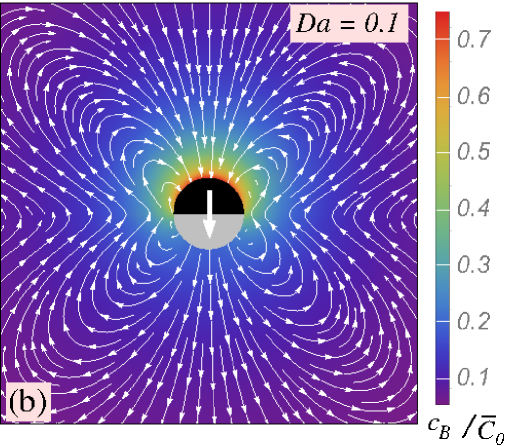
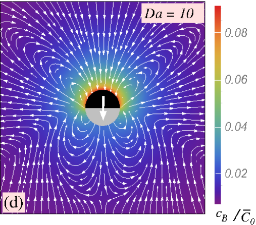
Figure 9: (a) The phoretic slip as a function of angular position $\theta$ [Eq. (10), truncated at the first 300 terms] for an active particle with chemical reaction of first order kinetics and $Da=0.1,~{}1,~{}\mathrm{and}~{}10$, respectively. (b)-(d) The force-free flow in the laboratory system (lines, Eqs. (13)) and the distribution of solute (color coded, Eq. (52)), for an active particle as in (a). For both the density and the flow the series are truncated after the first 50 terms. The thick white arrows at the particle show its direction of motion. In (a)-(d) the phoretic mobility is position independent and negative ($g(\theta)=-1$).

Figure 9(a) shows that the increase in the Damköhler number is correlated with an increasing asymmetry of the distribution of the phoretic slip along the surface: the larger the value of $Da$, the more sharply the phoretic slip is concentrated on the inert part. There are also visible changes in the magnitude of the phoretic slip. However, as emphasized above, the velocity scale $U_{0}$ itself depends on $Da$. The number density of product molecules (color coded background in Fig. 9(b)-(d)) mainly exhibits an overall change in magnitude upon increasing $Da$. (Note that also the density scale ${\bar{C}}_{0}$ itself depends on $Da$.) This translates into a reduced range of variations in $c$, consistent with the features in Fig. 9(a). On the other hand, the flow changes qualitatively. As expected, at $Da=10^{-1}$ the flow field is basically the one of a neutral squirmer (see the above discussion, Fig. 8(b), and Sec. III.1). Upon increasing the Damköhler number to $Da=1$ a front-back asymmetry of the flow pattern emerges, while further increasing the Damköhler number to $Da=10$ produces a clear puller-type flow, with a well defined stagnation point in front of the particle.

We conclude this section by remarking that the case of spatially varying phoretic mobilities can be straightforwardly addressed along the lines used for the models discussed in Sec. III.2. All necessary relations are provided in Sec. II.3. As in the other cases discussed in Sec. II.3, upon varying the sign and the magnitude of the mobilities on the active and inert parts, respectively, far-field hydrodynamic behaviors corresponding to a “pusher”, “puller”, “neutral”, or “shaker” particle can be observed.

V Effective interactions between active particles and between corresponding effective squirmers

The analyses in the previous sections illustrate the exact mapping of the hydrodynamic flow exhibited by various active colloids – suspended in an unbounded solution – onto effective hydrodynamic squirmers. Inter alia, for classical hydrodynamic squirmers an attractive or repulsive interaction between a squirmer and a wall can be used to infer a pusher, puller, or neutral character of the squirmer, respectively Spagnolie and Lauga (2012); Matas Navarro and Pagonabarraga (2010a). This naturally raises the question of whether the interaction of chemically active particles with confining boundaries (such as solid walls, fluid interfaces, inert particles, or other active colloids) can be captured – at least qualitatively – from the effective interaction with the same boundary of the corresponding effective squirmer (i.e., the one obtained via the mapping, as described in the previous sections, of the active particle in unbounded fluid). Moreover, one can further specify the above question as follows. Suppose that, e.g., an active particle exhibits, in the far field, an effective attractive or repulsive interaction with a wall. Can one then robustly infer from this observation that the effective squirmer corresponding to that particle (see above) has a pusher, puller, or neutral character Brown et al. (2016); Das et al. (2015)?

The complex behavior of the flow and of the particle motion depends sensitively on the details of both the chemical activity and the phoretic mobility. The analyses of this behavior in the previous sections point towards a negative answer to the above questions. The results in Sec. III.1 show that – up to an overall constant scale factor – identical flow patterns may emerge from seemingly different physical mechanisms of the chemical activity (e.g., the distinct models $(pi)$ and $(pa)$ are characterized by the same set of squirmer modes $B_{n}/B_{1}$). On the other hand, one can anticipate that the distinct mechanisms of activity will introduce distinct interactions with the boundary, obscuring the “effective squirmer” character of the mechanism of activity. In Sec. IV we have seen that changes in the importance of transport by diffusion relative to that of the reaction rate, i.e., the variation of the Damköhler number $Da$, may change the associated hydrodynamic flow from exhibiting a neutral squirmer character to a puller-like one. Finally, in Sec. III.2 we have seen that for a given chemical activity the character of the hydrodynamic flow induced by the active particle may vary across the whole spectrum of “pusher”, “puller”, and “neutral” behaviors via varying the pattern of phoretic mobility at the surface of the particle.

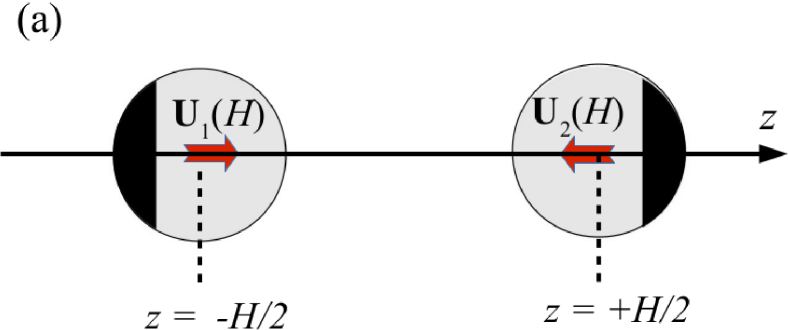
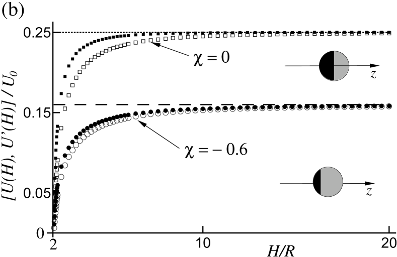
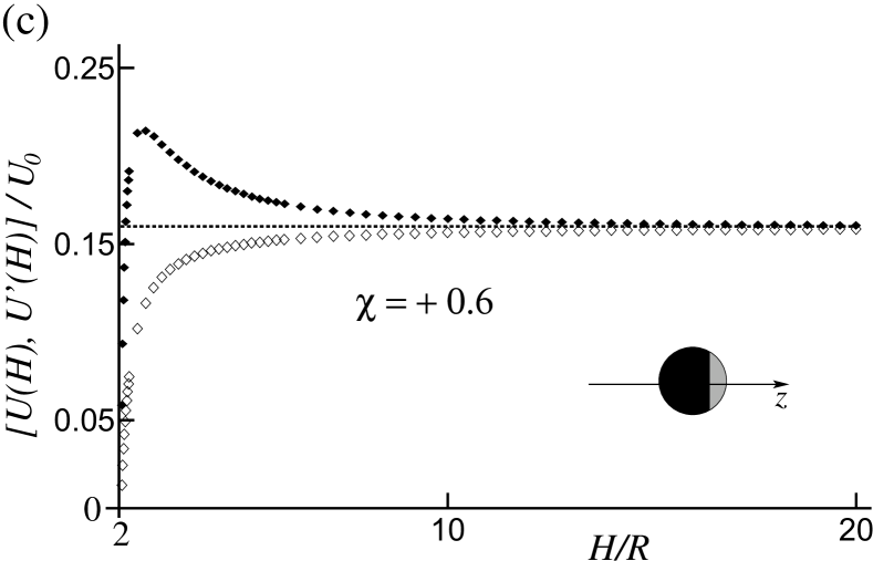
Figure 10: (a) Schematic diagram illustrating a central collision between two active particles of model $(pi)$ which are force and torque free. (b), (c) Velocity $U(H)$ (open symbols) of the active particle 1 and $U^{\prime}(H)$ (filled symbols) of the effective squirmer 1 (see the main text), respectively, in units of $U_{0}$. The results correspond to a position independent, negative phoretic mobility and to coverages (Eq. (56)) (b): $\chi=-0.6$ (effective “pusher”) and $0$ (effective “neutral”), and (c): $\chi=0.6$ (effective “puller”). The dashed line in (b) and the dotted lines in (b) and (c) indicate the value of the corresponding velocity $U^{(f)}(\chi)$ (Eq. (22)) of the particle in free space.

As a simple but insightful example, in this section we consider the set-up of the central collision between two identical active particles (i) belonging to model $(pi)$ with a position-independent phoretic mobility (see Fig. 10(a)), and their corresponding effective squirmer ersatz particles (ii). The results discussed below illustrate that there can be significant qualitative differences between the behaviors exhibited in the above two cases (i) and (ii). This implies that in the presence of geometrical confinements significant qualitative differences can exist between the behaviors exhibited by an active particle and by its corresponding “effective squirmer”, respectively. Therefore, the “inverse problem”, i.e., inferring a pusher, puller, or neutral character of the effective squirmer from the observation of a far-field attraction or repulsion of the active particle with a boundary, is in general ill-posed.

Turning to the example depicted schematically in Fig. 10(a), the two spherical, active particles are described by model $(pi)$ with a position-independent surface mobility (see the analysis in Sec. III.1); furthermore, we focus on the case that the particles are force and torque free. The number density $c(\mathbf{r})$ of solute molecules obeys the Laplace equation subject to the BC of solute-production at the catalytic caps (black areas in Fig. 10) on each of the two particles; it vanishes far from the particles. The hydrodynamic flow $\mathbf{u}(\mathbf{r})$ is the solution of the Stokes equations with the phoretic slip BC (Eq. (1)) which holds on each of the two particles and is determined by $c(\mathbf{r})$. The BC of a quiescent fluid applies far from the particles. Both these fields depend parametrically on $H=h/R$, where $h\geq 2R$ denotes the distance between the centers of the two particles of radius $R$. Due to symmetry, the two particles move along the $z$-axis, which connects their centers, with velocities $\mathbf{U}_{1,2}$ which are equal in magnitude but opposite in sign. $\mathbf{U}_{1,2}$ depend on $H$; for $H\to\infty$, the velocities take their corresponding values $\mathbf{U}^{(f)}$ for a single particle in an unbounded fluid (see Sec. III.1). The difference with the reference system of colliding “effective squirmers” is that for the latter the hydrodynamic slip at the surface is prescribed to be independent of $H$. It is set to that distribution which corresponds to the active particle as if it would be immersed in an unbounded fluid (see Eqs. (10), (19), and (21)). In order to discriminate between the active particles and the effective squirmer cases, we shall denote the corresponding velocities of the squirmers, which also depend on $H$, by a prime, i.e., $\mathbf{U}^{\prime}_{1,2}$.

Both boundary value problems (i.e., for the number density of the solute and for the hydrodynamic flow) can be solved exactly in terms of series representations in bi-polar coordinates Popescu et al. (2011); Papavassiliou and Alexander (2017); here we simply adapt and employ the solutions available in Refs. Domínguez et al. (2016); Malgaretti et al. (2018). We shall use the velocities of particle 1, $U_{1}(H):=U(H)>0$ and $U^{\prime}_{1}(H):=U^{\prime}(H)$, in order to characterize the effective interactions: an increase (decrease) relative to the free-space value $U^{(f)}=U(H\to\infty)\equiv U^{\prime}(H\to\infty)$ defines an effective attraction (repulsion) induced by the presence of particle $2$.

As discussed in Sec. III.1, the size of the catalytic cap is determined by the parameter

$$\chi=-\cos\theta_{0}\,,$$ (56)

which in the followings will be referred to as the coverage. For model $(pi)$ with a position independent phoretic mobility, this parameter allows one to tune the hydrodynamic flow of the active particle. For negative phoretic mobility the corresponding effective squirmer shows the far-field characteristics of a pusher for $\chi<0$, of a neutral squirmer for $\chi=0$, and of a puller for $\chi>0$ (see also Fig. 2(b)). We therefore choose suitable values for $\chi$ such that the model system under consideration exhibits each one of these desired behaviors.

The results $U(H)$ (open symbols) and $U^{\prime}(H)$ (filled symbols), in units of $U_{0}$ and corresponding to $\chi=-0.6$ (“pusher”) and $0$ (“neutral”) are shown in Fig. 10(b), while those corresponding to $\chi=0.6$ (“puller”) are shown in Fig. 10(c). While in the first two cases the somewhat naïve replacement of the active colloid with an effective squirmer results in a rather accurate approximation, in the last case this procedure fails. For $\chi=0.6$, the behavior is not only qualitatively different – the effective squirmers exhibit an attractive interaction, while the active colloids exhibit repulsion – but this qualitatively different behavior persists all the way to large separations $H$ (i.e., to the far field). However, this is not too surprising: it has been already pointed out in the literature (see, e.g., Refs. Golestanian et al. (2007); Uspal et al. (2015a); Simmchen et al. (2016)) that the distortions of the chemical field and those of the hydrodynamic flow induce, in general, changes in the velocity of the particle of the same order of decay as a function of the distance from the cause of distortions (boundary). As we show below, this is the case here, too. Accounting for both these distortions (rather than just for the hydrodynamic one, as it is the case for the effective squirmers) fully explains the effective repulsion exhibited in all cases by the active particle. Before we proceed, we re-emphasize that attributing the repulsion observed in Fig. 10(c) entirely to hydrodynamics and attempting to assign to this a type of squirmer leads to the erroneous inference of a “pusher” character. As a consequence, a follow-up analysis would attempt to find a surface activity such that it could be mapped onto an effective pusher, instead of searching for the correct “puller”-like mechanism (which is known to be the case for the active particle considered in Fig. 10(c)).

Focusing now solely on the results for the active particles, we look at providing a simple far-field approximation which allows one to understand their interaction. With this aim, we resort to a point particle approximation according to which we simply replace the second particle by the chemical, $c^{(2)}(\mathbf{r})$, and hydrodynamic flow field, $\mathbf{u}^{(2)}(\mathbf{r})$, which it produces as if it was single, and calculate the effects, in leading order, of these fields on particle 1. We start with the effects of the chemical field.

Colloid 1, located at $\mathbf{R}_{p}=(0,0,z=-H/2)$ in the external field $c^{(2)}(\mathbf{r})$ (see Eqs. (8) and (21) with the origin shifted to the point $(0,0,z=+H/2)$) acquires a phoretic velocity Anderson (1989)

$$\delta\mathbf{U}_{c}=(-b_{0})(\nabla c^{(2)})|_{\mathbf{r}=\mathbf{R}_{p}}\Rightarrow$$

$$\frac{\delta\mathbf{U}_{c}}{U_{0}}\simeq-\left\{f_{0}\left(\frac{R}{H}\right)^{2}-f_{1}\left(\frac{R}{H}\right)^{3}+{\cal O}\left[\left(\frac{R}{H}\right)^{4}\right]\right\}\mathbf{e}_{z}\,.$$

For the case of interest here, the particle is a net source of solute ($f_{0}\neq 0$) and the first term provides the leading order. However, there can be cases, such as the model activity $(pa)$ discussed in Sec. III, for which there is no net production (or annihilation), i.e., $f_{0}=0$. In such cases, the leading order term is the second one in the brackets. This latter term is proportional to $f_{1}$, which in turn determines the motility of the particle (see Eqs. (15) and (19)) and is nonzero for an active particle exhibiting motility in an unbounded solution.

We now turn to the effects of the flow $\mathbf{u}^{(2)}(\mathbf{r})$ on the motion of the particle 1. Faxén’s laws Happel and Brenner (1973) imply that, in the geometry shown in Fig. 10(a), particle 1 immersed in the flow $\mathbf{u}^{(2)}(\mathbf{r})$ (see Eq. (13) with $F=0$ and the origin shifted to the point $(0,0,z=+H/2)$) acquires the velocity Matas Navarro and Pagonabarraga (2010a, b); Ishikawa et al. (2006)

$$\delta\mathbf{U}_{h}=\mathbf{u}^{(2)}|_{\mathbf{r}=\mathbf{R}_{p}}\Rightarrow$$ (58)

$$\frac{\delta\mathbf{U}_{h}}{U_{0}}\simeq-\left[f_{2}\left(\frac{R}{H}\right)^{2}+\left(\frac{1}{3}f_{1}-\frac{3}{2}f_{3}\right)\left(\frac{R}{H}\right)^{3}\right]\mathbf{e}_{z}$$

$$\hskip 34.14322pt+\,{\cal O}\left[\left(\frac{R}{H}\right)^{4}\right]\mathbf{e}_{z}\,.$$ (59)

If the effective squirmer model, corresponding to the particle with uniform mobility, is either a pusher or a puller, one has $f_{2}\neq 0$ and the first term provides the leading order behavior (note that it has opposite signs for pusher and puller, respectively). On the other hand, if the effective squirmer mapping leads to a neutral squirmer, i.e., $f_{2}=0$, the first term vanishes and the leading order behavior is given by the second term, the amplitude of which involves both the modes $f_{1}$ and $f_{3}$ of the activity function.

Combining the two results above, and noting that $f_{0}>0$ for model $(pi)$ of interest here, one arrives at the following expression for the deviation $\delta\mathbf{U}$, at leading order, of the velocity of particle 1 from the “single-particle” value $U^{(f)}\mathbf{e}_{z}$:

$$\frac{\delta\mathbf{U}\cdot\mathbf{e}_{z}}{U_{0}} \simeq -\left(f_{0}+f_{2}\right)\left(\frac{R}{H}\right)^{2}$$

$$\overset{(pi)}{=} -\left(\frac{1+\chi}{2}-\frac{5}{4}\chi\sqrt{1-\chi^{2}}\right)\left(\frac{R}{H}\right)^{2}\,,$$

where in the last line we have specialized the more general result to the specific choice of the coefficients $f_{n}$ of model $(pi)$ (Eq. (21)).

Figure 11: The deviation of the velocity of particle 1 with radius $R$ from the “single particle” value $U^{(f)}$, in a central collision as depicted in Fig. 10(a), as function of the center-to-center separation $H/R$. The data correspond to a position independent, negative phoretic mobility and to coverages $\chi=\mp\,0.6$ (main panel), corresponding to an effective “pusher” or “puller”, respectively, and $\chi=0$ (inset), i.e., effectively “neutral”. The symbols show exact results obtained from series in terms of bi-polar coordinates; the data are taken from Figs. 10(b) and (c). The dashed and dotted lines show the corresponding predictions of the far-field approximation (Eq. (V)).

The first term in parentheses in the second line of Eq. (V), which accounts for the effective interaction induced by the chemical distortions, is positive and dominates the second one (which emerges from hydrodynamic interactions and changes sign at $\chi=0$) for all values of $-1<\chi<1$. Thus, the leading order far-field analysis above indeed correctly captures the main qualitative feature of the collision between these model active particles, in that they exhibit an effective repulsion irrespective of the coverage (see Figs. 10(b), 10(c), and 11). Furthermore, as can be seen in Fig. 11, in all three cases the predicted deviations from the single-particle velocity (Eq. (V)), i.e., the “effective interaction” between the two active particles, quantitatively capture the exact results at large values $H/R$, and, for $\chi\geq 0$, quasi-quantitatively down to separations as small as $H/R\gtrsim 4$ (see, also, similar reports on the accuracy of far-field approximations by, e.g., Ref. Spagnolie and Lauga (2012); Uspal et al. (2016, 2018)).

VI Summary and conclusions

We have analyzed in detail the connection between simple models of chemically active, spherical, axisymmetric particles moving by self-diffusiophoresis, as defined in Sects. II.1 and II.2, and the classic hydrodynamic squirmer model Lighthill (1952); Blake (1971).

For the motion in an unbounded fluid, this connection takes the form of an exact mapping from the model chemical activity and phoretic mobility of the particle to a set of squirming modes $B_{n}$, as reported previously Bickel et al. (2013); Michelin and Lauga (2014); Ibrahim and Liverpool (2016). For completeness, and because these results are somewhat isolated in the literature, the steps involved in constructing this mapping have been succinctly summarized in Sect. II.3. Such mappings provide the hydrodynamic flow around the active particle, i.e., the solution of the Stokes problem, in explicit form. Along the construction of this mapping, one finds as a by-product a simple derivation of the relation between the external force needed to immobilize the active particle (so-called “stall” force) and the velocity with which the particle would move in the absence of external forces (Eq. (17)).

In Sect. III we have illustrated such mappings for various, commonly used models of chemical activity and for particles with either position-independent or position-dependent phoretic mobility. For each case considered, the mapping was derived explicitly in terms of the functions describing the chemical activity and the phoretic mobility. The results have been illustrated as functions of geometrical parameters (e.g., the coverage) of the system and for various ratios of phoretic mobilities over the two parts of the particle surface: plots of (i) the number density of the solute, together with the associated hydrodynamic flow field, (ii) the distribution of the phoretic slip around the particle, and (iii) the sign and magnitude of the first two squirmer modes, based on which the particles can be classified as “pushers”, “pullers”, “neutral”, and, eventually, “shakers”. Two important conclusions have emerged from the examples discussed in Sect. III. The first is that the models of chemical activity involving arguably very distinct physical mechanisms, may map onto the same (up to a change of the velocity scale) effective squirmer (Sects. III.1.1. and III.1.2.). The second is that, for a given model of chemical activity, solely by varying the value of the ratio of phoretic mobilities over the two parts of the particle surface one arrives at effective squirmers which can exhibit any of the “pusher”, “puller”, or “neutral” characters (Sect. III.2). This highlights that even if the hydrodynamic flow around a squirmer is perfectly known, the pattern of chemical activity cannot be reliably and robustly inferred from it without knowing the phoretic mobility function and de-convoluting its contributions.

In Sect. IV we have shown how the mapping procedure can be straightforwardly extended to include the more complex case of a chemical reaction with a first order chemical kinetics. For the particular case of a Janus particle, this has been illustrated, in terms of number densities of the chemical species, the hydrodynamic flow field, and the slip distribution around the particle. By studying these at various values of the Damköhler number $Da$, which characterizes the relative importance of the transport by diffusion with respect to the reaction rate, we found changes in the resulting “effective” squirmer type from “neutral” at $Da\ll 1$ (reaction-limited kinetics) to “puller” at $Da\gg 1$ (diffusion-limited kinetics).

Finally, in order to build counter-examples, in Sect. V we have illustrated, by using the simple case of a central collision between two identical model active particles, that in the presence of geometric confinement it is not justified to replace the active particle by its effective squirmer, even if the interest is solely in the far-field behavior. Moreover, the examples shown in Figs. 10(b) and (c) highlight that attributing an observed effective interaction exhibited by the active particles entirely to hydrodynamics, and attempting to associate a type of squirmer based on such a hypothesis, may easily lead to flawed conclusions about the characteristics of a surface activity function compatible with that type of squirmer. While the direct use of the corresponding effective squirmer – if the particle operates under geometrical confinements – is thus unwise, the mapping onto an effective squirmer remains a very useful tool. By resorting to it, we have derived a far-field approximation (Eq. (V)) which rationalizes and captures (quasi)-quantitatively the effective interaction between the two active particles in the particular configuration shown in Fig. 11.

To conclude, we have highlighted both the advantages of the mapping of model chemically active colloids to effective hydrodynamic squirmers, as well as the drawbacks of unwarranted use of such approaches. As we have shown in Sect. V, carrying over the descriptions in terms of squirmers to studies of, e.g., the collective behavior in suspensions of active particles, is not well grounded even as an approximation of a “dilute limit” focused on far-field interactions. However, the success of the procedure in terms of effective interactions, which leads to Eq. (V), raises the intriguing question of whether similar results may hold in more complex, general situations. Such results would pave the way for finding simplified, yet robust and reliable models, to be employed, e.g., in large scale computer simulations of suspensions of active particles Wagner and Ripoll (2017); Delfau et al. (2016). We thus consider it as rewarding to study this issue in the context of more complex geometries, such as the motion of an active particle parallel or normal to an interface, or non-central binary collisions. For hydrodynamic squirmers in such geometries a wealth of results is available (see, e.g., Refs. Spagnolie and Lauga (2012); Matas Navarro and Pagonabarraga (2010a, b); Ishikawa et al. (2006); Ishimoto and Gaffney (2013)), which can facilitate a study as suggested above. Finally, we note that squirmer models are available for other axisymmetric shapes, such as prolate and oblate spheroids (see, e.g., Ref. Leshansky et al. (2007); Theers et al. (2016)), and thus similar mappings from chemically active particles to squirmers should also be possible for particles with elongated shapes (e.g., rods) as encountered in actual experimental studies.

Appendix A Useful relations

At various steps, the following relations Abramowitz and Stegun (1972) involving the Legendre polynomials $P_{n}$ and the associated Legendre functions $P_{n}^{m}$ of degree $n$ and order $m=1$ have been used:

$$P_{n}^{1}(\cos\theta):=-\sin\theta\,\frac{dP_{n}(\cos\theta)}{d(\cos\theta)}=\frac{dP_{n}(\cos\theta)}{d\theta}\,,$$ (61)

$$\int\limits_{0}^{\pi}d\theta\sin\theta P_{n}(\cos\theta)P_{k}(\cos\theta)=\frac{2}{(2n+1)}\,\delta_{n,k}\,,$$ (62)

$$\int\limits_{0}^{\pi}d\theta\sin\theta P_{n}^{1}(\cos\theta)P_{k}^{1}(\cos\theta)=\frac{2n(n+1)}{(2n+1)}\,\delta_{n,k}\,,$$ (63)

and

$${\cal H}_{n}(\omega_{0}:=\cos\theta_{0}):=\int\limits_{\omega_{0}}^{1}duP_{n}(u)$$ (64)

$$\hskip 28.45274pt=\begin{cases}1-\omega_{0}\,,&n=0\,,\\ ~{}~{}\\ -\frac{(1-\omega_{0}^{2})^{1/2}}{n(n+1)}P_{n}^{1}(\omega_{0})\,,&n\geq 1\,.\end{cases}$$

For $m\neq n$, one has

$$H_{n,m}(\omega_{0}:=\cos\theta_{0}):=\int\limits_{\omega_{0}}^{1}duP_{m}(u)P_{n}(u)$$ (65)

$$\hskip 28.45274pt=-(1-\omega_{0}^{2})^{1/2}\,\,\frac{P_{n}(\omega_{0})P_{m}^{1}(\omega_{0})-P_{m}(\omega_{0})P_{n}^{1}(\omega_{0})}{m(m+1)-n(n+1)}\,.$$

References

- Ismagilov et al. (2002) R.F. Ismagilov, A. Schwartz, N. Bowden, and G.M. Whitesides, “Autonomous movement and self-assembly,” Angew. Chem. Int. Ed. 41, 652–654 (2002).
- Paxton et al. (2004) W.F. Paxton, K.C. Kistler, C.C. Olmeda, A. Sen, S.K. St. Angelo, Y.Y. Cao, T.E. Mallouk, P.E. Lammert, and V.H. Crespi, “Catalytic nanomotors: Autonomous movement of striped nanorods,” J. Am. Chem. Soc. 126, 13424–13431 (2004).
- Ozin et al. (2005) G.A. Ozin, I. Manners, S. Fournier-Bidoz, and A. Arsenault, “Dream nanomachines,” Adv. Mater. 17, 3011–3018 (2005).
- Paxton et al. (2006a) W.F. Paxton, S. Sundararajan, T.E. Mallouk, and A. Sen, “Chemical locomotion,” Angew. Chem. Int. Ed. 45, 5420–5429 (2006a).
- Paxton et al. (2006b) W.F. Paxton, P.T. Baker, T.R. Kline, Y. Wang, T.E. Mallouk, and A. Sen, “Catalytically induced electrokinetics for motors and micropumps,” J. Am. Chem. Soc. 128, 14881–14888 (2006b).
- Solovev et al. (2009) A.A. Solovev, Y.F. Mei, E.B. Urena, G.S. Huang, and O.G. Schmidt, “Catalytic microtubular jet engines self-propelled by accumulated gas bubbles,” Small 5, 1688–1692 (2009).
- Mirkovic et al. (2010) T. Mirkovic, N.S. Zacharia, G.D. Scholes, and G.A. Ozin, “Nanolocomotion - catalytic nanomotors and nanorotors,” Small 6, 159–167 (2010).
- Fournier-Bidoz et al. (2005) S. Fournier-Bidoz, A.C. Arsenault, I. Manners, and G.A. Ozin, “Synthetic self-propelled nanorotors,” Chem. Commun. , 441–443 (2005).
- Howse et al. (2007) J.R. Howse, R.A.L. Jones, A.J. Ryan, T. Gough, R. Vafabakhsh, and R. Golestanian, “Self-motile colloidal particles: From directed propulsion to random walk,” Phys. Rev. Lett. 99, 048102:1–4 (2007).
- Volpe et al. (2011) G. Volpe, I. Buttinoni, D. Vogt, H.-J. Kümmerer, and C. Bechinger, “Microswimmers in patterned environments,” Soft Matter 7, 8810–8815 (2011).
- Ebbens et al. (2012) S. Ebbens, M.-H. Tu, J.R. Howse, and R. Golestanian, “Size dependence of the propulsion velocity for catalytic Janus-sphere swimmers,” Phys. Rev. E 85, 020401(R):1–4 (2012).
- Kümmel et al. (2013) F. Kümmel, B. ten Hagen, R. Wittkowski, I. Buttinoni, R. Eichhorn, G. Volpe, H. Löwen, and C. Bechinger, “Circular motion of asymmetric self-propelling particles,” Phys. Rev. Lett. 110, 198302:1–5 (2013).
- Buttinoni et al. (2013) I. Buttinoni, J. Bialké, F. Kümmel, H. Löwen, C. Bechinger, and T. Speck, “Dynamical clustering and phase separation in suspensions of self-propelled colloidal particles,” Phys. Rev. Lett. 110, 238301:1–5 (2013).
- Lee et al. (2014) T.-C. Lee, M. Alarcón-Correa, C. Miksch, K. Hahn, J.G. Gibbs, and P. Fischer, “Self-propelling nanomotors in the presence of strong Brownian forces,” Nano Lett. 14, 2407–2412 (2014).
- Ebbens et al. (2014) S. Ebbens, D.A. Gregory, G. Dunderdale, J.R. Howse, Y. Ibrahim, T.B. Liverpool, and R. Golestanian, “Electrokinetic effects in catalytic Pt-insulator Janus swimmers,” EPL 106, 58003:1–6 (2014).
- ten Hagen et al. (2014) B. ten Hagen, F. Kümmel, R. Wittkowski, D. Takagi, H. Löwen, and C. Bechinger, “Gravitaxis of asymmetric self-propelled colloidal particles,” Nature Comm. 5, 4829:1–7 (2014).
- Ma et al. (2016) X. Ma, S. Jang, M.N. Popescu, W.E. Uspal, A. Miguel-López, K. Hahn, D.-P. Kim, and S. Sánchez, “Reversed Janus micro/nanomotors with internal chemical engine,” ACS Nano 10, 8751–8759 (2016).
- Herminghaus et al. (2014) S. Herminghaus, C.C. Maas, C. Krüger, S. Thutupalli, L. Goehring, and C. Bahr, “Interfacial mechanisms in active emulsions,” Soft Matter 10, 7008–7022 (2014).
- Seemann et al. (2016) R. Seemann, J.-B. Fleury, and C.C. Maas, “Self-propelled droplets,” Eur. Phys. J. Special Topics 225, 2227–2240 (2016).
- Kroy et al. (2016) K. Kroy, D. Chakraborty, and F. Cichos, “Hot microswimmers,” Eur. Phys. J. Special Topics 225, 2207–2226 (2016).
- Lozano et al. (2016) C. Lozano, B. ten Hagen, H. Löwen, and C. Bechinger, “Phototaxis of synthetic microswimmers in optical landscapes,” Nature Comm. 7, 12828:1–10 (2016).
- Golestanian et al. (2005) R. Golestanian, T.B. Liverpool, and A. Ajdari, “Propulsion of a molecular machine by asymmetric distribution of reaction products,” Phys. Rev. Lett. 94, 220801:1–4 (2005).
- Golestanian et al. (2007) R. Golestanian, T.B. Liverpool, and A. Ajdari, “Designing phoretic micro- and nano-swimmers,” New J. Phys. 9, 126:1–8 (2007).
- Rückner and Kapral (2007) G.R. Rückner and R. Kapral, “Chemically powered nanodimers,” Phys. Rev. Lett. 98, 150603:1–4 (2007).
- Jülicher and Prost (2009) F. Jülicher and J. Prost, “Generic theory of colloidal transport,” Eur. Phys. J. E 29, 27–36 (2009).
- Popescu et al. (2011) M.N. Popescu, M. Tasinkevych, and S. Dietrich, “Pulling and pushing a cargo with a catalytically active carrier,” EPL 95, 28004:1–6 (2011).
- Sabass and Seifert (2012a) B. Sabass and U. Seifert, “Dynamics and efficiency of a self-propelled, diffusiophoretic swimmer,” J. Chem. Phys. 136, 064508:1–15 (2012a).
- Sabass and Seifert (2012b) B. Sabass and U. Seifert, “Nonlinear, electrocatalytic swimming in the presence of salt,” J. Chem. Phys. 136, 214507:1–13 (2012b).
- Kapral (2013) R. Kapral, “Nanomotors without moving parts that propel themselves in solution,” J. Chem. Phys. 138, 202901:1–10 (2013).
- Sharifi-Mood et al. (2013) N. Sharifi-Mood, J. Koplik, and C. Maldarelli, “Diffusiophoretic self-propulsion of colloids driven by a surface reaction: The sub-micron particle regime for exponential and van der Waals interactions,” Phys. Fluids 25, 012001:1–34 (2013).
- ten Hagen et al. (2011) B. ten Hagen, S. van Teeffelen, and H. Löwen, “Brownian motion of a self-propelled particle,” J. Phys.: Condens. Matter 23, 194119:1–12 (2011).
- Michelin and Lauga (2015) S. Michelin and E. Lauga, “Autophoretic locomotion from geometric asymmetry,” Eur. Phys. J. E 38, 7:1–16 (2015).
- Hu et al. (2015) J. Hu, A. Wysocki, R.G. Winkler, and G. Gompper, “Physical sensing of surface properties by microswimmers - directing bacterial motion via wall slip,” Sci. Rep. 5, 9586:1–7 (2015).
- Popescu et al. (2016) M.N. Popescu, W.E. Uspal, and S. Dietrich, “Self-diffusiophoresis of chemically active coloids,” Eur. Phys. J. Special Topics 225, 2189–2206 (2016).
- Zöttl and Stark (2016) A. Zöttl and H. Stark, “Emergent behavior in active colloids,” J. Phys.: Condens. Matter 28, 253001:1–28 (2016).
- de Graaf et al. (2015) J. de Graaf, G. Rempfer, and C. Holm, “Diffusiophoretic self-propulsion for partially catalytic spherical colloids,” IEEE Trans. NanoBiosci. 14, 272–288 (2015).
- Oshanin et al. (2017) G. Oshanin, M.N. Popescu, and S. Dietrich, “Active colloids in the context of chemical kinetics,” J. Phys. A 50, 134001:1–50 (2017).
- Lammert et al. (2016) P.E. Lammert, V.H. Crespi, and A. Nourhani, “Bypassing slip velocity: rotational and translational velocities of autophoretic colloids in terms of surface flux,” J. Fluid Mech. 802, 294–304 (2016).
- Brown et al. (2017) A.T. Brown, W.C.K. Poon, C. Holm, and J. de Graaf, “Ionic screening and dissociation are crucial for understanding chemical self-propulsion in polar solvents,” Soft Matter 13, 1200–1222 (2017).
- Lauga and Powers (2009) E. Lauga and T.R. Powers, “The hydrodynamics of swimming microorganisms,” Rep. Prog. Phys. 72, 096601:1–36 (2009).
- Ebbens and Howse (2010) S.J. Ebbens and J.R. Howse, “In pursuit of propulsion at the nanoscale,” Soft Matter 6, 726–738 (2010).
- Hong et al. (2010) Y. Hong, D. Velegol, N. Chaturvedi, and A. Sen, “Biomimetic behavior of synthetic particles: from microscopic randomness to macroscopic control,” Phys. Chem. Chem. Phys. 12, 1423–1435 (2010).
- Elgeti et al. (2015) J. Elgeti, R.G. Winkler, and G. Gompper, “Physics of microswimmers – single particle motion and collective behavior: a review,” Rep. Prog. Phys. 78, 056601:1–50 (2015).
- Bechinger et al. (2016) C. Bechinger, R. Di Leonardo, H. Löwen, C. Reichhardt, G. Volpe, and G. Volpe, “Active particles in complex and crowded environments,” Rev. Mod. Phys. 88, 045006:1–50 (2016).
- Moran and Posner (2016) J.L. Moran and J.D. Posner, “Phoretic self-propulsion,” Ann. Rev. Fluid Mech. 49, 511–540 (2016).
- Derjaguin et al. (1966) B.V. Derjaguin, Yu.I. Yalamov, and A.I. Storozhilova, “Diffusiophoresis of large aerosol particles,” J. Colloid Interface Sci. 22, 117–125 (1966).
- Anderson (1989) J.L. Anderson, “Colloid transport by interfacial forces,” Ann. Rev. Fluid Mech. 21, 61–99 (1989).
- Pozrikidis (2002) C. Pozrikidis, A Practical Guide to Boundary Element Methods with the Software Library BEMLIB (CRC Press, Boca Raton, 2002).
- Happel and Brenner (1973) J. Happel and H. Brenner, Low Reynolds number hydrodynamics (Noordhoff Int. Pub., Leyden, The Netherlands, 1973).
- Lighthill (1952) M.J. Lighthill, “On the squirming motion of nearly spherical deformable bodies through liquids at very small Reynolds numbers,” Commun. Pure App. Math. 5, 109–118 (1952).
- Blake (1971) J.R. Blake, “A spherical envelope approach to ciliary propulsion,” J. Fluid Mech. 46, 199–208 (1971).
- Pak and Lauga (2014) O.S. Pak and E. Lauga, “Generalized squirming motion of a sphere,” J. Eng. Math. 88, 1–28 (2014).
- Lauga et al. (2006) E. Lauga, W.R. DiLuzio, G.M. Whitesides, and H.A. Stone, “Swimming in circles: Motion of bacteria near solid boundaries,” Biophys. J. 90, 400–412 (2006).
- Berke et al. (2008) A.P. Berke, L. Turner, H.C. Berg, and E. Lauga, “Hydrodynamic attraction of swimming microorganisms by surfaces,” Phys. Rev. Lett. 101, 038102:1–4 (2008).
- Drescher et al. (2010) K. Drescher, R.E. Goldstein, N. Michel, M. Polin, and I. Tuval, “Direct measurement of the flow field around swimming microorganisms,” Phys. Rev. Lett. 105, 168101:1–4 (2010).
- Lopez and Lauga (2014) D. Lopez and E. Lauga, “Dynamics of swimming bacteria at complex interfaces,” Phys. Fluids 26, 071902:1–23 (2014).
- Mathijssen et al. (2016) A.J.T.M. Mathijssen, A. Doostmohammadi, J.M. Yeomans, and T.N. Shendruk, “Hydrodynamics of micro-swimmers in films,” J. Fluid Mech. 806, 35–70 (2016).
- Matas Navarro and Pagonabarraga (2010a) R. Matas Navarro and I. Pagonabarraga, “Hydrodynamic interactions in squirmer motion: swimming with a neighbour and close to a wall,” J. Non-Newtonian Fluid Mech. 165, 946–952 (2010a).
- Ishimoto and Gaffney (2013) K. Ishimoto and E.A. Gaffney, “Squirmer dynamics near a boundary,” Phys. Rev. E 88, 062702:1–12 (2013).
- de Graaf et al. (2016) J. de Graaf, A.J.T.M. Mathijssen, M. Fabritius, H. Menke, C. Holm, and T.N. Shendruk, “Understanding the onset of oscillatory swimming in microchannels,” Soft Matter 12, 4704–4708 (2016).
- Lintuvuori et al. (2016) J.S. Lintuvuori, A.T. Brown, K. Stratford, and D. Marenduzzo, “Hydrodynamic oscillations and variable swimming speed in squirmers close to repulsive walls,” Soft Matter 12, 7959–7968 (2016).
- Spagnolie and Lauga (2012) S. Spagnolie and E. Lauga, “Hydrodynamics of self-propulsion near a boundary: predictions and accuracy of far-field approximations,” J. Fluid Mech. 700, 105–147 (2012).
- Spagnolie et al. (2015) S.E. Spagnolie, G.R. Moreno-Flores, D. Bartolo, and E. Lauga, “Geometric capture and escape of a microswimmer colliding with an obstacle,” Soft Matter 11, 3396–3411 (2015).
- Takagi et al. (2014) D. Takagi, J. Palacci, A.B. Braunschweig, M.J. Shelley, and J. Zhang, “Hydrodynamic capture of microswimmers into sphere-bound orbits,” Soft Matter 10, 1784–1789 (2014).
- Ishikawa et al. (2006) T. Ishikawa, M.P. Simmonds, and T.J. Pedley, “Hydrodynamic interaction of two swimming model micro-organisms,” J. Fluid Mech. 568, 119–160 (2006).
- Papavassiliou and Alexander (2017) D. Papavassiliou and G.P. Alexander, “Exact solutions for hydrodynamic interactions of two squirming spheres,” J. Fluid Mech. 813, 618–646 (2017).
- Matas Navarro and Pagonabarraga (2010b) R. Matas Navarro and I. Pagonabarraga, “Hydrodynamic interaction between two trapped swimming model micro-organisms,” Eur. Phys. J. E 33, 27–39 (2010b).
- Alarcón and Pagonabarraga (2013) F. Alarcón and I. Pagonabarraga, “Spontaneous aggregation and global polar ordering in squirmer suspensions,” J. Molecular Liquids 185, 56–61 (2013).
- Delfau et al. (2016) J.-B. Delfau, J. Molina, and M. Sano, “Collective behavior of strongly confined suspensions of squirmers,” EPL 114, 24001:1–6 (2016).
- Saintillan and Shelley (2008) D. Saintillan and M.J. Shelley, “Instabilities, pattern formation, and mixing in active suspensions,” Phys. Fluids 20, 123304:1–16 (2008).
- Lauga and Nadal (2016) E. Lauga and F. Nadal, “Clustering instability of focused swimmers,” EPL 116, 64004:1–6 (2016).
- Bickel et al. (2013) T. Bickel, A. Majee, and A. Würger, “Flow pattern in the vicinity of self-propelling hot Janus particles,” Phys. Rev. E 88, 012301:1–6 (2013).
- Michelin and Lauga (2014) S. Michelin and E. Lauga, “Phoretic self-propulsion at finite Peclét numbers,” J. Fluid Mech. 747, 572–604 (2014).
- Ibrahim and Liverpool (2016) Y. Ibrahim and T.B. Liverpool, “How walls affect the dynamics of self-phoretic microswimmers,” Eur. Phys. J. Special Topics 225, 1843–1874 (2016).
- Baraban et al. (2012) L. Baraban, M. Tasinkevych, M.N. Popescu, S. Sánchez, S. Dietrich, and O.G. Schmidt, “Transport of cargo by catalytic Janus micro-motors,” Soft Matter 8, 48–52 (2012).
- Palacci et al. (2013) J. Palacci, S. Sacanna, A.S. Steinberg, D.J. Pine, and P.M. Chaikin, “Living crystals of light-activated colloidal surfers,” Science 339, 936–940 (2013).
- Uspal et al. (2015a) W.E. Uspal, M.N. Popescu, S. Dietrich, and M. Tasinkevych, “Self-propulsion of a catalytically active particle near a planar wall: from reflection to sliding and hovering,” Soft Matter 11, 434–438 (2015a).
- Mozaffari et al. (2016) A. Mozaffari, N. Sharifi-Mood, J. Koplik, and C. Maldarelli, “Self-diffusiophoretic colloidal propulsion near a solid boundary,” Phys. Fluids 28, 053107:1–35 (2016).
- Brown et al. (2016) A.T. Brown, I.D. Vladescu, A. Dawson, T. Vissers, J. Schwarz-Linek, J.S. Lintuvuori, and W.C.K. Poon, “Swimming in a crystal,” Soft Matter 12, 131–140 (2016).
- Leshansky et al. (1997) A.M. Leshansky, A.A. Golovin, and A. Nir, “Thermocapillary interaction between a solid particle and a liquid-gas interface,” Phys. Fluids 9, 2818–2827 (1997).
- Domínguez et al. (2016) A. Domínguez, P. Malgaretti, M.N. Popescu, and S. Dietrich, “Effective interaction between active colloids and fluid interfaces induced by Marangoni flows,” Phys. Rev. Lett. 116, 078301:1–5 (2016).
- Das et al. (2015) S. Das, A. Garg, A.I. Campbell, J.R. Howse, A. Sen, D. Velegol, R. Golestanian, and S.J. Ebbens, “Boundaries can steer active Janus spheres,” Nature Comm. 6, 8999:1–10 (2015).
- Simmchen et al. (2016) J. Simmchen, J. Katuri, W.E. Uspal, M.N. Popescu, M. Tasinkevych, and S. Sánchez, “Topographical pathways guide chemical microswimmers,” Nature Comm. 7, 10598:1–9 (2016).
- Uspal et al. (2016) W.E. Uspal, M.N. Popescu, S. Dietrich, and M. Tasinkevych, “Guiding catalytically active particles with chemically patterned surfaces,” Phys. Rev. Lett. 117, 048002:1–5 (2016).
- Popescu et al. (2017a) M.N. Popescu, W.E. Uspal, and S. Dietrich, “Chemically active colloids near osmotic-responsive walls with surface-chemistry gradients,” J. Phys.: Condens. Matter 29, 134001:1–13 (2017a).
- Uspal et al. (2018) W.E. Uspal, M.N. Popescu, M. Tasinkevych, and S. Dietrich, “Shape-dependent guidance of active Janus particles by chemically patterned surfaces,” New J. Phys. 20, 015013 (2018).
- Liu et al. (2016) C. Liu, C. Zhou, W. Wang, and H.P. Zhang, “Bimetallic microswimmers speed up in confining channels,” Phys. Rev. Lett. 117, 198001:1–6 (2016).
- Popescu et al. (2009) M.N. Popescu, S. Dietrich, and G. Oshanin, “Confinement effects on diffusiophoretic self-propellers,” J. Chem. Phys. 130, 194702:1–16 (2009).
- Uspal et al. (2015b) W.E. Uspal, M.N. Popescu, S. Dietrich, and M. Tasinkevych, “Rheotaxis of spherical active particles near a planar wall,” Soft Matter 11, 6613–6632 (2015b).
- Katuri et al. (2018) J. Katuri, W.E. Uspal, J. Simmchen, A. Miguel López, and S. Sánchez, “Cross-stream migration of active particles,” Sci. Adv. 4, eaao1755 (2018).
- Campbell and Ebbens (2013) A.I. Campbell and S.J. Ebbens, “Gravitaxis in spherical Janus swimming devices,” Langmuir 29, 14066–14073 (2013).
- Enculescu and Stark (2011) M. Enculescu and H. Stark, “Active colloidal suspensions exhibit polar order under gravity,” Phys. Rev. Lett. 107, 058301:1–5 (2011).
- Ibrahim and Liverpool (2015) Y. Ibrahim and T.B. Liverpool, “The dynamics of a self-phoretic Janus swimmer near a wall,” EPL 111, 48008:1–6 (2015).
- Popescu et al. (2017b) M.N. Popescu, W.E. Uspal, M. Tasinkevych, and S. Dietrich, “Perils of ad hoc approximations for the activity function of chemically powered colloids,” Eur. Phys. J. E 40, 42:1–7 (2017b).
- Sharifi-Mood et al. (2016) N. Sharifi-Mood, A. Mozaffari, and U.M. Córdova-Figueroa, “Pair interaction of catalytically active colloids: from assembly to escape,” J. Fluid Mech. 798, 910–954 (2016).
- Reigh and R. (2015) S.Y. Reigh and Kapral R., “Catalytic dimer nanomotors: continuum theory and microscopic dynamics,” Soft Matter 11, 3149–3158 (2015).
- Popescu et al. (2010) M.N. Popescu, S. Dietrich, M. Tasinkevych, and J. Ralston, “Phoretic motion of spheroidal particles due to self-generated solute gradients,” Eur. Phys. J. E 31, 351–367 (2010).
- Brady (2011) J.F. Brady, “Particle motion driven by solute gradients with application to autonomous motion: Continuum and colloidal perspectives,” J. Fluid Mech. 667, 216–259 (2011).
- de Groot and Mazur (1962) S.R. de Groot and P. Mazur, Non-equilibrium Thermodynamics (North-Holland, Amsterdam, 1962).
- Abramowitz and Stegun (1972) M. Abramowitz and I.R. Stegun, Eds. Handbook of mathematical functions (Dover, New York, 1972).
- Ma et al. (2015) X. Ma, A. Jannasch, U.-R. Albrecht, K. Hahn, A. Miguel-López, E. Schäffer, and S. Sánchez, “Enzyme-powered hollow mesoporous Janus nanomotors,” Nano Lett. 15, 7043–7050 (2015).
- Eskandari (2016) Z. Eskandari, “Head-on collisions of chemically active colloids,” (2016), unpublished .
- Brown and Poon (2014) A. Brown and W. Poon, “Ionic effects in self-propelled Pt-coated Janus swimmers,” Soft Matter 10, 4016–4027 (2014).
- Córdova-Figueroa and Brady (2008) Ubaldo M. Córdova-Figueroa and John F. Brady, “Osmotic propulsion: The osmotic motor,” Phys. Rev. Lett. 100, 158303:1–4 (2008).
- Collins (1961) W.D. Collins, “On some dual series equations and their application to electrostatic problems for spheroidal caps,” Math. Proc. Cambridge Phil. Soc. 57, 367–384 (1961).
- Sneddon (1966) I.N. Sneddon, Mixed boundary Value in Potential Theory (North-Holland, Amsterdam, The Netherlands, 1966).
- Samson and Deutch (1978) R. Samson and J.M. Deutch, “Diffusion-controlled reaction rate to a buried active site,” J. Chem. Phys. 68, 285–290 (1978).
- Shoup et al. (1981) D. Shoup, G. Lipari, and A. Szabo, “Diffusion-controlled bimolecular reaction rates. The effect of rotational diffusion and orientation constraints,” Biophys. J. 36, 697–714 (1981).
- Shoup and Szabo (1982) D. Shoup and A. Szabo, “Role of diffusion in ligand binding to macromolecules and cell-bound receptors,” Biophys. J. 40, 33–39 (1982).
- Traytak (1994) S.D. Traytak, “The steric factor in the time-dependent diffusion-controlled reactions,” J. Phys. Chem. 98, 7419–7421 (1994).
- Traytak (1995) S.D. Traytak, “Diffusion-controlled reaction rate to an active site,” Chem. Phys. 192, 1–7 (1995).
- Traytak and Tachiya (1995a) S.D. Traytak and M. Tachiya, “Diffusion-controlled reaction rate to asymmetric reactants under Coulomb interaction,” J. Chem. Phys. 102, 9240–9247 (1995a).
- Traytak and Tachiya (1995b) S.D. Traytak and M. Tachiya, “Diffusion-controlled reaction rate to an active site in an external electric field,” J. Chem. Phys. 102, 2760–2771 (1995b).
- Traytak and Price (2007) S.D. Traytak and W.S. Price, “Exact solution for anisotropic diffusion-controlled reactions with partially reflecting conditions,” J. Chem. Phys. 127, 184508:1–8 (2007).
- Malgaretti et al. (2018) P. Malgaretti, M.N. Popescu, and S. Dietrich, “Self-diffusiophoresis induced by fluid interfaces,” Soft Matter 14, 1375–1388 (2018).
- Wagner and Ripoll (2017) M. Wagner and M. Ripoll, “Hydrodynamic front-like swarming of phoretically active dimeric colloids,” EPL 119, 66007:1–7 (2017).
- Leshansky et al. (2007) A.M. Leshansky, O. Kenneth, O. Gat, and J.E. Avron, “A frictionless microswimmer,” New J. Phys. 9, 145:1–17 (2007).
- Theers et al. (2016) M. Theers, E. Westphal, G. Gompper, and R. G. Winkler, “Modeling a spheroidal microswimmer and cooperative swimming in a narrow slit,” Soft Matter 12, 7372–7385 (2016).