Magnetic phase diagram of the strongly frustrated quantum spin chain system PbCuSO₄(OH)₂ in tilted magnetic fields.

Abstract

We report the $\mathbf{H}-T$ phase diagram of $S=1/2$ strongly frustrated anisotropic spin chain material linarite PbCuSO₄(OH)₂ in tilted magnetic fields up to 10 T and temperatures down to 0.2 K. By means of torque magnetometry we investigate the phase diagram evolution as the magnetic field undergoes rotation in $\mathbf{ba}^{\ast}$ and $\mathbf{bc}$ planes. The key finding is the robustness of the high field spin density wave-like phase, which may persist even as the external field goes orthogonal to the chain direction $\mathbf{b}$. In contrast, the intermediate collinear antiferromagnetic phase collapses at moderate deflection angles with respect to $\mathbf{b}$ axis.

I Introduction

Frustrated quantum magnets host extreme quantum fluctuations that enable a variety of exotic novel phases of spin matter Zhitomirsky et al. (2000); Shannon et al. (2006); Sudan et al. (2009); Balents and Starykh (2016). Much attention has been given to even the simplest of models, namely the Heisenberg $S=1/2$ spin chain with ferromagnetic $J_{1}$ and next-nearest neighbor antiferromagnetic $J_{2}$ interactions Sudan et al. (2009); Zhitomirsky and Tsunetsugu (2010); Sato et al. (2013). While quantum fluctuations destabilize the semiclassical spin spiral order, substantial ferromagnetic interactions favor the formation of magnon bound states. In applied magnetic fields the bounds states may condense before single magnons do. The result is the so-called bond-nematic phase with no dipolar magnetic order, yet spontaneously broken spin rotational symmetry Andreev and Grishchuk (1984); Zhitomirsky et al. (2000). Other unusual quantum phases, such as complicated spiral structures or spin density waves (SDW) have also been predicted Sudan et al. (2009); Sato et al. (2013); Nishimoto et al. (2015).

One of the most intriguing potential experimental realizations of this model  Baran et al. (2006); Willenberg et al. (2012) is the natural mineral linarite PbCuSO₄(OH)₂ (see Fig. 1). It combines pronounced frustration with very convenient energy scales: in the exchange interactions between Cu²⁺ $S=1/2$ ions in linarite are $J_{1}\simeq-14.5$ and $J_{2}\simeq 3.93$ meV resulting in a saturation field below $10$ T. The thermodynamic properties are rather exotic: for the field applied along the chain direction one finds up to 5 distinct magnetic phases below $T_{N}\simeq 2.7$ K Willenberg et al. (2016). Among them there is especially peculiar high field phase, which was identified as the longitudinal SDW. The latter was argued to be a possible precursor to the magnon pair condensate, or possibly even the phase separation between such a condensate and a conventional dipolar order Sudan et al. (2009); Willenberg et al. (2016).

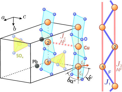
Figure 1: The crystal structure of linarite PbCuSO₄(OH)₂. The main exchange interactions (competing ferromagnetic $J_{1}$ and antiferromagnetic $J_{2}$, and interchain $J_{c}$) are indicated. The anisotropy axes $\vec{\xi}_{1}\parallel\mathbf{b}$ and $\vec{\xi}_{2}$ in the $\mathbf{ac}$ plane are also shown together with the range of magnetic field directions, studied in the present work.

Any discussion of linarite in the context of purely isotropic $J_{1}-J_{2}$ chain model Willenberg et al. (2016); Rule et al. (2017) is incomplete. Magnetic anisotropy certainly plays a role in this material, as evidenced by the dramatic difference in the phase diagrams measured for field applied parallel and perpendicular to the chain axis Schäpers et al. (2013); Povarov et al. (2016). Anisotropy effects were recently addressed in an experimental and theoretical study Cemal et al. (2018). It was shown that the magnetically ordered structures can be understood in terms of mean field model with orthorhombic (biaxial) anisotropy included. The theoretical description also accounted for a significant mismatch between the magnetic anisotropy and crystal lattice directions. The proposed easy and middle axes of the anisotropy are indicated as $\vec{\xi}_{1}$ and $\vec{\xi}_{2}$ vectors in Fig. 1. Unfortunately, the available experimental data Cemal et al. (2018) are either restricted to relatively high temperatures or specific directions of the magnetic field. A complete orientational low-temperature magnetic phase diagram of linarite is still lacking.

In the present study we use low-temperature torque magnetometry to map out this phase diagram for arbitrary magnetic field directions in $\mathbf{ba}^{\ast}$ and $\mathbf{bc}$ planes. This allows us to trace the evolution of each of the magnetic phases as the field is rotated away from the easy axis direction. Special attention is paid to the high field phase which we find to be very robust, in contrast with the fragile intermediate field Neél phase.

II Experimental

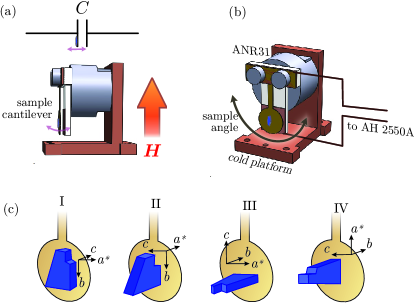
Figure 2: Schematics of the custom probe used in the measurements. (a) Principle of the torque measurement: probe senses the force, acting on the sample in the vertical magnetic field $\mathbf{H}$, by change of the capacitance between the brass cantilever and the base copper pad due to the deflection of the former. A Stycast 1226 panel (shown in white) provides an electric insulation between the effective capacitor parts. (b) The overview of the probe: the capacitance $C$ of the torque probe is measured by the capacitance bridge AH 2550A, while the angle between the field and cantilever principal axis (and hence the sample) can be tuned by the ANR31 rotator (gray). The complete assembly is fixed on a copper beryllium rack and mounted on the DR cold platform. (c) Four different measurement geometries used in the present study.

The challenge is to map out the sub-K magnetic phase diagram of a strongly anisotropic system, featuring many transitions that substantially affect the magnetization $\mathbf{M}$. This makes torque magnetometry a very advantageous probe. In our particular realization the sample is attached to the free end of a cantilever, $\mathbf{L}$ being the vector from its fixed point to the sample. Then the torque acting on the cantilever free end consists of two terms:

$$\mathcal{T}=\mathcal{T}_{\perp}+\mathcal{T}_{\parallel}=[\mathbf{M}\times\mathbf{H}]+[\mathbf{L}\times(\mathbf{M}\cdot\nabla)\mathbf{H}].$$ (1)

The $\mathcal{T}_{\perp}$ term depends only on the magnetization component that is transverse to the magnetic field $\mathbf{H}$. The other term $\mathcal{T}_{\parallel}$ is mostly sensitive to the component along the field. Therefore, the method probes the changes in both longitudinal and transverse components of the uniform magnetization, and this sensitivity progressively increases with the external field magnitude. On the down side, the the field gradient dependence in $\mathcal{T}_{\parallel}$ (which would vary depending on the magnet used or the precise sample position) makes the data difficult to interpret quantitatively. As we will show below, for the purposes of this study this is not a concern, as the transition-related features are conspicuously pronounced in the data, and a simple qualitative interpretation is sufficient to reconstruct the phase boundaries.

A schematic of a custom torquemeter probe used in this work is shown in Figs. 2(a,b). The sample is attached to the pad of the cantilever made of of $0.1$ mm thick brass foil. We measure the cantilever deflection (i.e. the torque force component normal to the pad) by observing a change in the electric capacitance $C$ between the pad and the fixed copper plate. The typical capacitance of the probe is about $0.5$ pF, and the typical deflection-induced change is within $1$% of this value. The capacitance $C$ is measured directly with the help of Andeen-Hagerling 2550A capacitance bridge. The probe is in turn mounted onto the Attocube ANR31 rotator, providing the ability to adjust the angle between the sample and the magnetic field. The measurement unit (Fig. 2b) is attached to the cold platform of the Quantum Design Dilution Refrigerator option (DR), that is used in a Quantum Design Physical Property Measurement System (PPMS) equipped with a 14 T superconducting magnet. A similar PPMS system with a 9 T magnet was also used in some of the measurements.

For the study we have used a small $m\simeq 20$ mg natural linarite single crystal (originating from Grand Reef Mine, Arizona, USA). This crystal belongs to the same batch as the samples from the previous study Povarov et al. (2016). Although some mechanically induced shape irregularities, two good facets given by $\mathbf{bc}$ and $\mathbf{a}^{\ast}\mathbf{c}$ lattice vectors are present. The linear dimensions of the crystal are approximately $3\times 2\times 1$ mm along $\mathbf{b}$, $\mathbf{a}^{\ast}$, $\mathbf{c}$. The crystal was placed onto the cantilever pad in four different configurations shown in Fig. 2(c). The adjustment of the rotator position was always done at the room temperature, as the rotator calibration is temperature-dependent. Initial positioning of the crystal on the cantilever pad is the biggest source of experimental uncertainty in the magnetic field angle. We estimate the offset that may occur during the initial positioning as not exceeding $\pm 3^{\circ}$. This offset is constant within the series of measurements in a given configuration. The error resulting from readjusting the rotator angle is negligible in comparison.

Capacitance $C(H)$ measurements were done at a set of fixed temperatures (0.2 K lowest) with the magnetic field being swept at 20 Oe/sec.

The intrinsic demagnetizing fields of linarite do not exceed 0.1 T, and are thus comparable to the typical width of the features that will be discussed below .

III Results and discussion

III.1 Torque curve and the phase transitions

The raw $\Delta C(H)=C(H)-C(0)$ curves have rather complicated shape greatly varying depending on the magnetic field direction. The most structured curves occur at $\mathbf{H}\parallel\mathbf{b}$, the chain direction. The left panels of Fig. 3 shows the data, recorded in two different configurations featuring the same field orientation $\mathbf{H}\parallel\mathbf{b}$. Right panels are the corresponding $dC/dH$ derivatives. Despite that the curves from configuration I and II appear very different at the first glance, they show a number of robust features. These allow us to reproduce the well-known phase boundaries for $\bf{H}\|\bf{b}$  Schäpers et al. (2013, 2014); Willenberg et al. (2016); Povarov et al. (2016); Cemal et al. (2018).

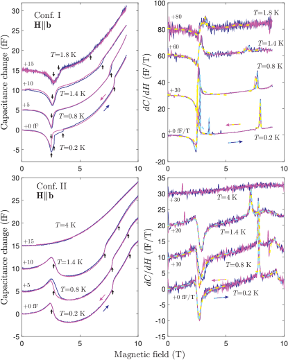
Figure 3: Selected $\Delta C(H)$ torque curves and their derivatives for $\mathbf{H}\parallel\mathbf{b}$ in configurations I (upper panels) and II (lower panels). The temperatures and offsets are indicated in the plots. Solid lines are the data; dashed lines are the fits given by Eqs. (2,3,4). Vertical arrows mark the obtained transition fields.

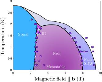
Figure 4: Magnetic $\mathbf{H}\parallel\mathbf{b}$ phase diagram of linarite, measured in configurations I (circles) and II (squares). The filled and hollow points correspond to down and up field sweeps. The solid lines correspond to the previously published phase diagram Willenberg et al. (2016); Povarov et al. (2016). Phases are labeled according to Cemal et al. (2018).

First of all, there is a low field peak-like anomaly (dip or peak around $H\simeq 3$ T), corresponding to the transition between the spin spiral and commensurate structure . This feature is rather asymmetric; however, its derivative can be conveniently described by the distorted Lorentzian function:

$$\frac{dC}{dH}=aH+b+\frac{I_{0}\sigma^{2}}{\sigma^{2}+(H-H_{0})^{2}}\left(1-\frac{\alpha}{\sigma}(H-H_{0})\right)$$ (2)

Most of the parameters in the above formula are purely empirical: the linear background coefficients $a$ and $b$, the anomaly “amplitude” $I_{0}$ and the asymmetry coefficient $\alpha$. Physically meaningful parameters are the peak center $H_{0}$ that is the transition field and width $\sigma$ that is considered as twice the experimental uncertainty.

Second, at low temperatures the broad feature may be superimposed with abrupt discontinuous jumps, as is the case for $T=0.2$ K curve in configuration I around $H\simeq 3.5$ T(Fig. 3). It is important to note that these jumps always have extremely hysteretic character and are mostly present in the sweeps with increasing magnetic field. A convenient way of fitting the jump-like features is to approximate the peak-like derivative with a Gaussian function, superimposed with linear background:

$$\frac{dC}{dH}=aH+b+\frac{I_{0}}{\sigma\sqrt{2\pi}}\text{exp}\left(\frac{-(H-H_{0})^{2}}{2\sigma^{2}}\right).$$ (3)

Again, $a$ and $b$ describe the linear background and $I_{0}$ is the Gaussian amplitude. Transition field and experimental error are given by $H_{0}$ and $0.5\sigma$ correspondingly.

The third type of features are the “smoothed” jumps, which mark the lower boundary of the most interesting high field phase. Again, the derivative of these features is well described by a biased Gaussian function (3).

Finally, the saturation field manifests itself as an apparent kink in the $\Delta C(H)$ curve. Again, a convenient way to pinpoint the transition field is an empirical approximation of the derivative with some peak-like function. Biased Gaussian (3) may serve as a good candidate, however we find that in many cases the “smoothed angle” describes the cusp in the derivative more accurately. It is defined as follows:

$$y(x) = a_{1}x+b_{1},x\leq H_{0},$$ (4)

$$y(x) = a_{2}(x-H_{0})+a_{1}H_{0}+b_{1},x>H_{0},$$

$$\frac{dC}{dH} = \int\limits_{-\infty}^{+\infty}y(x)\frac{1}{\sigma\sqrt{2\pi}}\text{exp}\left(\frac{-(H-x)^{2}}{2\sigma^{2}}\right)dx.$$

The above definition simply describes two straight lines forming a sharp angle at the anomaly position $H_{0}$, and then convoluted with the Gaussian of width $\sigma$. As before, this width is a good estimate for the experimental uncertainty.

In both configurations all features show some temperature dependence. At $T>T_{N}$ (e.g. $4$ K curve in Fig. 3) the $\Delta C(H)$ data become absolutely featureless, confirming the magnetic order origin of the anomalies at lower temperatures. Importantly, the highest-field anomaly is very sensitive to the temperature and becomes almost unobservable above 1 K. This is a general property of the enigmatic “Fan/SDW” phase: it has very weak thermodynamic manifestations at finite $T$ and therefore becomes hardly distinguishable from a fully polarized state. Empirically this sets $1.4$ K as the threshold temperature at which this phase of main interest can be resolved.

The result of treating the $\mathbf{H}\parallel\mathbf{b}$ data is summarized in Fig. 4. We certainly can reproduce the entire known phase diagram. The agreement between the data measured in two different geometries (configurations I and II) is an additional self-consistency check for our experimental approach.

III.2 Evolution in tilted magnetic field

As the magnetic field gets deflected from the $\mathbf{b}$ axis towards the $\mathbf{c}$ direction, the torque $\Delta C(H)$ curves undergo substantial changes. The most obvious but least informative trend is the deformation of overall shape of the curves. It largely depends on the multiple geometrical factors in Eq. (1) that are at least partially beyond the experimental control. The really valuable information is contained in the changing $\Delta C(H)$ anomalies.

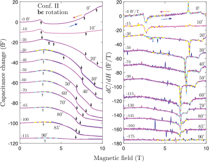
Figure 5: Evolution of the $\Delta C(H)$ torque signal as the magnetic field is rotated in the $\mathbf{bc}$ plane. The measurement geometry is configuration II. Selected torque curves and their derivatives at $T=0.2$ K are plotted as solid lines in the left and right panels correspondingly. The angles and offsets are indicated in the plots. Dashed lines indicate various anomalies approximated by Eqs. (2-5) as described in the main text. Vertical arrows mark the obtained fields (black — transitions, gray — crossovers).

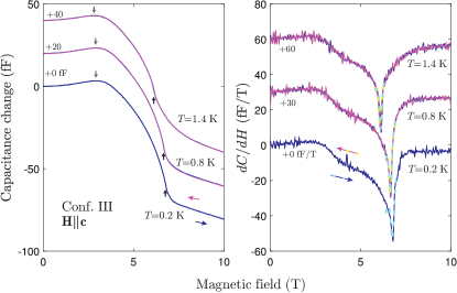
Figure 6: Selected $\Delta C(H)$ curves and their derivatives for $\mathbf{H}\parallel\mathbf{c}$ (configuration III). The temperatures and offsets are indicated in the plots. Dashed lines indicate various anomalies approximated by Eqs. (3,5) as described in the main text. Vertical arrows mark the obtained fields (black — transitions, gray — crossovers).

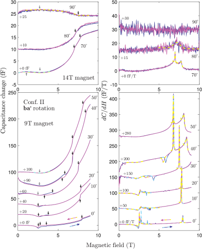
Figure 7: Evolution of the $\Delta C(H)$ torque signal as the magnetic field is rotated in the $\mathbf{ba}^{\ast}$ plane. The measurement geometry is configuration I. Selected torque curves and their derivatives at $T=0.2$ K are plotted as solid lines in the left and right panels correspondingly. The angles and offsets are indicated in the plots. Upper and lower set of panels contain the data recorded with 14 T or 9 T magnet, correspondingly. Dashed lines indicate various anomalies approximated by Eqs. (2-5) as described in the main text. Vertical arrows mark the obtained fields (black — transitions, gray — crossovers).

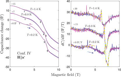
Figure 8: Selected $\Delta C(H)$ curves and their derivatives for $\mathbf{H}\parallel\mathbf{a}^{\ast}$ (configuration IV). The temperatures and offsets are indicated in the plots. Dashed lines indicate various anomalies approximated by Eqs. (2,3) as described in the main text. Vertical arrows mark the obtained fields (black — transitions, gray — crossovers).

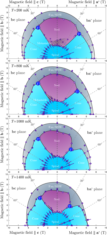
Figure 9: Angular phase diagram of linarite in $\mathbf{bc}$ and $\mathbf{ba}^{\ast}$ planes. Symbols correspond to the positions of the anomalies in the torque data; hollow symbols for sweeping the field up and filled symbols for sweeping the field down. Different symbol shapes correspond to different measurement configurations: circles, squares, downward and upward triangles — for setups I, II, III and IV correspondingly. Lines are guide to the eye. Circles labeled with “T?” mark the regions where the tricritical point is expected.

The first thing that is happening as the cantilever is rotated is the shift of the anomalies positions. This is the manifestation of shifting magnetic phase boundaries. Second, the apparent amplitudes of the anomalies may change as well. There are both intrinsic and extrinsic reasons for this. The anomalies may indeed become less pronounced as certain phases become suppressed and the corresponding order parameter vanishes. On the other hand, the cantilever sensitivity depends on the geometry which may or may not be favorable. For example, at $10^{\circ}$ tilt towards $\mathbf{c}$ (see the corresponding curve in Fig. 5) the forces acting on the cantilever become rather compensated in the deflection direction, resulting in a very weak signal. Consistently, the deflection of the cantilever goes inwards or outwards for smaller or larger field tilts. Nonetheless, in terms of transition-related anomalies the evolution is smooth until $30^{\circ}$ where the sharp wiggle related to the transition between spiral and commensurate states is gone.

At higher tilt angles this feature gives way to a broad maximum in $\Delta C(H)$. This maximum continues to carry useful information on the spin structure. The non-monotonous character of the curve signals a competition between forces resulting from transverse and longitudinal magnetization components in Eq. (1). As for a given run the geometry is fixed, the maximum (or minimum) in the deflection signals the change of balance between $\mathbf{M}\parallel\mathbf{H}$ and $\mathbf{M}\perp\mathbf{H}$ components, and hence a significant reorientation of the spin structure. It looks much more like a crossover than a proper phase transition, as the associated feature is quite broad. We can empirically describe it as a simple parabola:

$$\Delta C(H)=b\pm\left(\frac{H-H_{0}}{\sigma}\right)^{2}.$$ (5)

Again, $b$ is the purely empirical offset with no physical meaning, while $H_{0}$ and $\sigma$ serve as the feature center and width estimate. We can guess that such anomaly corresponds to a transformation from a “flat” zero-field spin spiral into a cone phase with significant polarization along the field direction. This reorientation feature persists in the data all the way to the fully transverse field geometry.

We can also resolve the anomalies corresponding to the boundaries of the high field phase at least up to $85^{\circ}$. The enigmatic “Fan/SDW” phase persists, although it shrinks as the field comes to the transverse orientation. In the fully transverse geometry with $\mathbf{H}\parallel\mathbf{c}$ in configuration II the signal is again dramatically reduced and it is impossible to draw any conclusions about the presence of the high field phase. This motivated us to use an additional geometry III, with $\mathbf{H}\parallel\mathbf{c}$ being in the sensitive torquemeter configuration. The results are shown in Fig. 6. The conclusion is that within the experimental resolution one observes just one high field anomaly even at the lowest temperatures and the high field phase is absent for $\mathbf{H}\parallel\mathbf{c}$ exact orientation.

A similar sequence of events is happening in case of magnetic field tilt from $\mathbf{b}$ to $\mathbf{a}^{\ast}$ as shown in Fig. 7. The quantitative difference is that the Neél phase is somewhat more robust in this case and holds until $40^{\circ}$ tilt. As the low-tilt series of data were measured in a machine with a 9 T magnet, we are also missing the high field saturation anomaly in some of these curves, as it was simply out of the accessible range. However, it finally appears below 9 T as the tilt exceeds $30^{\circ}$. We are able to trace the boundaries of the high field phase up to $70^{\circ}$; for higher tilts the signal-to-noise screens the fine structure of the high field anomaly. Again, this can be overcome by employing the sensitive geometry IV with $\mathbf{H}\parallel\mathbf{a}^{\ast}$. The results are shown in Fig. 8. Surprisingly, in this case we find the high field phase present and clearly resolved.

The data from all the measurements at all the temperatures is summarized in a series of angular phase diagrams present in Fig. 9. They will be discussed in detail in the next section.

IV Discussion

The main result of this study is the angular phase diagrams in Fig. 9, which can be briefly summarized as follows: the Neél phase is rather fragile and vanishes at approximately $40^{\circ}$ tilt from the $\mathbf{b}-$axis, while the enigmatic “Fan/SDW” phase that precedes full saturation turns out to be robust and may indeed persist even in the transverse magnetic field orientation. Both findings are qualitatively consistent with the theoretical predictions of Cemal et al. Cemal et al. (2018). In particular, in the close to $a$ direction of magnetic field we do observe a non-vanishing high field phase, in agreement with the direct observations of the “Fan” state by Cemal et al.. Unfortunately, the static uniform magnetization measurements do not provide us with any microscopic information, and thus it is not possible to differentiate between the “Fan” and “SDW” possibilities from our set of data to extend this comparison further.

Fig. 9 also plots the crossover from “flat” zero-field spiral to the partially polarized cone state. As discussed above, on this line the structure becomes predominantly polarized along the field around $2.8-3$ T, in agreement with neutron diffraction data Cemal et al. (2018). While in the neutron diffraction data this microscopic change of structure is rather sharp and pronounced, in torque magnetometry measurements it appears as a broad crossover. This loosely defined crossover field is replaced by a sharp transition in the narrow angular range supporting the collinear Neél phase. Metastability effects stress the first order nature of that transition. Interestingly, in the exact $\mathbf{H}\parallel\mathbf{b}$ orientation history-dependent behavior is confined to the lowest temperatures, while with the deflection towards the $\mathbf{c}$-axis they start to proliferate and become present in the whole temperature range of the study. As soon as the Neél phase ceases to exist, any history dependent behavior disappears.

An important observation is that the field at which the flat spin spiral structure is transformed, either through a crossover or a phase transition, is nearly the same for all orientations. This tells us that the same energy scale is at play, that is the main easy axis anisotropy ($\vec{\xi}_{1}\parallel\mathbf{b}$ direction in Fig. 1). On the other hand, the Neél phase is supposedly stabilized by the smaller anisotropy constant (associated with the $\vec{\xi}_{2}$ direction) Cemal et al. (2018). Thus, knowing the critical angles at which the collinear phase disappears may be essential to get an estimate of both anisotropy energies.

An interesting minor detail is the behavior of “triple” points separating the Neél, high field and cone phases. Although we do not have enough angular resolution to locate these points precisely (their possible locations are indicated by large circles in Fig.  9), it seems that around these points the stability of the high field phase is enhanced. This behavior is particularly pronounced at higher temperatures.

Another minor point concerns the intermediate small pocket of “phase III” Willenberg et al. (2016); Povarov et al. (2016) which is found at higher temperatures for $\mathbf{H}\parallel\mathbf{b}$ (as in Fig. 4). In our experiments it could not be clearly resolved in any other orientations and is therefore not indicated in the Fig. 9 phase diagrams.

V Conclusions

The complex orientational magnetic phase diagram of linarite reflects a subtle competition between anisotropy terms in the magnetic Hamiltonian. Nevertheless, it is not at all inconsistent with the “big picture” of competing quantum phases in the simplified $J_{1}-J_{2}$ Heisenberg model. On a qualitative level, our findings are consistent with the mean field model of Ref. Cemal et al. (2018). Further theoretical work is needed to enable a quantitative comparison.