Energy Minimization for Wireless Communication with Rotary-Wing UAV

Abstract

This paper studies unmanned aerial vehicle (UAV) enabled wireless communication, where a rotary-wing UAV is dispatched to send/collect data to/from multiple ground nodes (GNs). We aim to minimize the total UAV energy consumption, including both propulsion energy and communication related energy, while satisfying the communication throughput requirement of each GN. To this end, we first derive an analytical propulsion power consumption model for rotary-wing UAVs, and then formulate the energy minimization problem by jointly optimizing the UAV trajectory and communication time allocation among GNs, as well as the total mission completion time. The problem is difficult to be optimally solved, as it is non-convex and involves infinitely many variables over time. To tackle this problem, we first consider the simple fly-hover-communicate design, where the UAV successively visits a set of hovering locations and communicates with one corresponding GN when hovering at each location. For this design, we propose an efficient algorithm to optimize the hovering locations and durations, as well as the flying trajectory connecting these hovering locations, by leveraging the travelling salesman problem (TSP) and convex optimization techniques. Next, we consider the general case where the UAV communicates also when flying. We propose a new path discretization method to transform the original problem into a discretized equivalent with a finite number of optimization variables, for which we obtain a locally optimal solution by applying the successive convex approximation (SCA) technique. Numerical results show the significant performance gains of the proposed designs over benchmark schemes, in achieving energy-efficient communication with rotary-wing UAVs.

UAV communication, rotary-wing UAV, energy model, energy-efficient communication, trajectory optimization, path discretization.

I Introduction

Wireless communication using unmanned aerial platforms is a promising technology to achieve wireless coverage in areas without or with insufficient terrestrial infrastructures. Early efforts have been primarily focusing on using high altitude platforms (HAPs), which are deployed in stratosphere at altitude around 20 km, aiming to provide ubiquitous coverage in rural or remote areas. These include the Project Loon by Google with the mission of “Balloon-powered Internet for everyone”, as well as the Project Skybender by Google and the Project Aquila by Facebook, both using solar-powered drones to provide internet access from the sky. On the other hand, wireless communication using low altitude platforms (LAPs), typically below a few kilometers above the ground, has received growing interests recently. LAPs can be implemented in various ways, such as helikite [1] and unmanned aerial vehicles (UAVs) [2, 3, 4, 5, 6]. In particular, compared to other airborne solutions such as HAPs and helikite, UAV-enabled wireless communication brings new advantages [2], such as on-demand and more swift deployment, superior link quality in the presence of shorter-distance line-of-sight (LoS) communication channel with ground nodes (GNs), and higher network flexibility with the fully controllable UAV movement in three dimensional (3D) airspace. Therefore, UAV-enabled wireless communication has many potential use cases, including public safety communication, temporary traffic offloading for cellular base stations (BSs), information dissemination and data collection for Internet of Things (IoTs), as well as emergency response and fast service recovery after natural disasters.

Prior researches on UAV-enabled wireless communications can be loosely classified into two categories. In the first category, UAVs are deployed as (quasi-)stationary aerial BSs. In this case, UAVs resemble the conventional static terrestrial BSs, but at a much higher altitude and thus possesses new channel characteristics [7, 8, 9, 10, 11]. In particular, it was shown that as the UAV altitude increases, the LoS probability between the UAV and GNs also increases [12]. By exploiting such unique channel characteristics, significant efforts have been devoted to studying the various aspects of UAV-enabled BSs, such as UAV placement optimization [12, 13, 14, 15, 16, 17], performance analysis [18, 19, 20], spectrum sharing [21], and cell association [22]. In contrast, the other category considers the application scenarios where UAVs are employed as mobile BSs/relays/access points (APs) [23, 24, 25, 26, 27, 28], whose trajectories can be designed to optimize the communication performance. For example, a UAV as a mobile relay or data collector can fly closer to its associated GNs for communication to improve the overall spectrum efficiency [23] and/or save the communication energy of GNs [26]. In [23], a new framework of joint power allocation and UAV trajectory optimization was proposed for the UAV-enabled mobile relaying system, which has been extended to various other setups such as UAV-enabled data collection [26], multi-UAV coordinated/cooperative communication [27], [29], and UAV-enabled wireless power transfer [30].

One critical issue of UAV-enabled wireless communication lies in the limited on-board energy of UAVs [2], which needs to be efficiently used to enhance the communication performance and prolong the UAV’s endurance. Compared to conventional terrestrial BSs, UAVs incur additional propulsion energy consumption to maintain airborne and support their movement. In practice, the UAV propulsion power is usually much higher than the communication related power. As a result, the energy-efficient wireless communication design with UAV is significantly different from that in conventional terrestrial communication systems. An initial attempt for designing energy-efficient UAV communication via trajectory optimization was made in [25], where the energy efficiency in bits/Joule of a fixed-wing UAV enabled communication system is maximized for a given flight duration. To that end, a generic energy model as a function of the UAV’s velocity and acceleration was derived for fixed-wing UAVs. Based on the energy model in [25], the authors in [31] further revealed an interesting trade-off between UAV’s energy consumption and that of the GNs it communicating with. However, the above results for fixed-wing UAVs cannot be applied for rotary-wing UAVs, due to their fundamentally different mechanical designs and hence drastically different propulsion energy models. This thus motivates our current work to investigate energy-efficient communication for rotary-wing UAVs.

In this paper, we study a wireless communication system enabled a rotary-wing UAV. Compared to fixed-wing UAVs, rotary-wing UAVs have several appealing advantages such as the ability to take off and land vertically, as well as for hovering, which render them more popular in the current UAV market. We consider the scenario where a rotary-wing UAV is dispatched as a flying AP to communicate with multiple GNs, each of which has a target number of information bits to be transmitted/received to/from the UAV. Such a setup corresponds to many practical applications, such as UAV-enabled data collection for periodic sensing, UAV-enabled caching where the UAV pre-fetches the data and then transmits to the designated caching nodes [32], etc. Our objective is to minimize the UAV’s energy consumption, including both propulsion energy and communication energy, while ensuring that the communication requirement for each GN is satisfied. The main contributions of this paper are summarized as follows.

First, we derive an analytical model for the propulsion power consumption of rotary-wing UAVs, based on the results in aircraft literature [33], [34]. As expected, the obtained model is significantly different from that for fixed-wing UAVs derived in our prior work [25].

Based on the derived power consumption model, we formulate the energy minimization problem that jointly optimizes the UAV trajectory, the communication time allocation among the multiple GNs, as well as the total mission completion time. The problem is difficult to be optimally solved, as it is non-convex and constitutes infinite number of optimization variables that are coupled in continuous functions over time. To tackle this problem, we first consider the simple fly-hover-communicate design [17] to gain useful insights. Under this design, the UAV successively visits a set of optimized hovering locations, and communicates with each of the GNs only when hovering at the corresponding location. In this case, the problem reduces to finding the optimal hovering locations and hovering duration at each location, as well as the visiting order and flying speed among these locations. The problem is still NP hard, as it includes the classic NP hard travelling salesman problem (TSP) as a special case [35]. By leveraging the existing TSP-solving algorithm [36] and convex optimization techniques, an efficient high-quality approximate solution is obtained for our problem.

Next, we propose a general solution to the energy minimization problem where the UAV communicates also when flying. To this end, we first propose a novel discretization technique, called path discretization, to transform the original problem with infinitely many variables into a more tractable form with a finite number of variables. Different from the widely used time discretization approach for UAV trajectory design (see e.g. [23] and [25]), path discretization does not require the mission completion time to be pre-specified. This is particularly useful for problems where the mission completion time is also one of the optimization variables, as for the energy minimization problem studied in this paper. However, the path-discretized problem is still non-convex, and thus it is challenging to find its optimal solution. By utilizing the successive convex approximation (SCA) technique [23], an efficient iterative algorithm is proposed to simultaneously update the UAV trajectory and communication time allocation at each iteration, which is guaranteed to converge to at least a locally optimal solution satisfying the Karush-Kuhn-Tucker (KKT) conditions. Last, simulation results are provided to validate the proposed designs and show their significant performance gains over benchmark schemes.

It is worth noting that another related line of work is on mobile robotics, which exploits the mobility of ground robots for various applications [37], [38]. However, the design for UAV communication systems are significantly different from that for ground robotics due to the distinct air-to-ground channel characteristics [7, 8, 9, 10, 11] as well as the fundamentally different energy consumption models. For example, the power consumption of mobile robots can usually be modeled as a polynomial and monotonically increasing function with respect to its moving speed [37], which is much simpler than that for fixed-wing UAVs as in [25] and rotary-wing UAVs in Section II-B of the current work.

II System Model and Problem Formulation

II-A System Model

We consider a wireless communication system where a rotary-wing UAV is dispatched to communicate with $K$ GNs, which are denoted by the set $\mathcal{K}=\{1,\cdots,K\}$. The horizontal location of the GN $k\in\mathcal{K}$ is denoted as $\mathbf{w}_{k}\in\mathbb{R}^{2\times 1}$. We assume that the UAV flies at a constant altitude $H$ and the total number of information bits that need to be communicated with GN $k$ is $\tilde{Q}_{k}$. Let $T_{t}$ denote the total time required for the UAV to complete the mission, which is a design variable. Denote by $\mathbf{q}(t)\in\mathbb{R}^{2\times 1}$ with $0\leq t\leq T_{t}$ the UAV trajectory projected onto the horizontal plane. Let $V_{\max}$ denote the maximum UAV speed. We then have the constraint $\|\dot{\mathbf{q}}(t)\|\leq V_{\max}$. At any time instant $t\in[0,T_{t}]$, the distance between the UAV and GN $k$ is given by $d_{k}(t)=\sqrt{H^{2}+\|\mathbf{q}(t)-\mathbf{w}_{k}\|^{2}},\ k\in\mathcal{K}$.

We assume that the wireless channels between the UAV and GNs are dominated by LoS links. Thus, the channel power gain between the UAV and GT $k$ can be modeled based on the free-space path loss model as

$$h_{k}(t)=\beta_{0}d_{k}^{-2}(t)=\frac{\beta_{0}}{H^{2}+\|\mathbf{q}(t)-\mathbf{w}_{k}\|^{2}},$$ (1)

where $\beta_{0}$ represents the channel power gain at the reference distance of $1$ meter (m). Furthermore, assuming a fixed transmission power $P$ by the transmitter when it is scheduled for communication, the achievable rate in bits per second (bps) between GN $k$ and the UAV at any time instant $t$ is expressed as

$$R_{k}(t) =B\log_{2}\left(1+\frac{Ph_{k}(t)}{\sigma^{2}\Gamma}\right)=B\log_{2}\left(1+\frac{\gamma_{0}}{H^{2}+\|\mathbf{q}(t)-\mathbf{w}_{k}\|^{2}}\right),$$ (2)

where $B$ denotes the channel bandwidth in hertz (Hz), $\sigma^{2}$ is the noise power at the receiver, $\Gamma>1$ accounts for the gap from the channel capacity due to the practical modulation and coding scheme employed, and $\gamma_{0}\triangleq P\beta_{0}/(\sigma^{2}\Gamma)$ is defined as the received signal-to-noise ratio (SNR) at the reference distance of $1$ m.

We assume that the time-division multiple access (TDMA) protocol is applied for the UAV to serve the $K$ GNs, in order to fully exploit the time-varying channels with trajectory design. Let a binary variable $\lambda_{k}(t)\in\{0,1\}$ denote the user scheduling indicator at time instant $t$, with $\lambda_{k}(t)=1$ indicating that GN $k$ is scheduled for communication at instant $t$ and $\lambda_{k}(t)=0$ otherwise. As at most one GN can be scheduled at each time instant $t$, we have

$$\sum_{k=1}^{K}\lambda_{k}(t)\leq 1,\forall t\in[0,T_{t}].$$ (3)

Therefore, the aggregated communication throughput for GN $k$ is a function of $T_{t}$, $\mathbf{q}(t)$, and $\lambda_{k}(t)$, which can be expressed as

$$\bar{R}_{k} \big{(}T_{t},\{\mathbf{q}(t)\},\{\lambda_{k}(t)\}\big{)}=\int_{0}^{T_{t}}\lambda_{k}(t)R_{k}(t)dt$$

$$=B\int_{0}^{T_{t}}\lambda_{k}(t)\log_{2}\left(1+\frac{\gamma_{0}}{H^{2}+\|\mathbf{q}(t)-\mathbf{w}_{k}\|^{2}}\right)dt.$$ (4)

To ensure the target communication throughput requirement for each GN $k$, we must have

$$\bar{R}_{k}\big{(}T_{t},\{\mathbf{q}(t)\},\{\lambda_{k}(t)\}\big{)}\geq\tilde{Q}_{k},\ \forall k\in\mathcal{K}.$$ (5)

II-B Energy Consumption Model for Rotary-Wing UAV

The UAV energy consumption is in general composed of two main components, namely the communication related energy and the propulsion energy. The communication related energy includes that for communication circuitry, signal processing, signal radiation/reception, etc. In this paper, we assume that the communication related power is a constant, which is denoted as $P_{c}$ in watt (W). On the other hand, the propulsion energy consumption is needed to keep the UAV aloft and support its movement, if necessary. In general, the propulsion energy depends on the UAV flying speed as well as its acceleration. In this paper, for the purpose of exposition and drawing the essential design insight, we ignore the additional energy consumption caused by UAV acceleration, which is valid for typical communication applications where UAV manoeuvring time only takes a small portion of the total operation time. As derived in Appendix A, for a rotary-wing UAV flying with speed $V$, the propulsion power consumption can be modeled as

$$P(V)= \underbrace{P_{0}\left(1+\frac{3V^{2}}{U_{\mathrm{tip}}^{2}}\right)}_{\text{blade profile}}+\underbrace{P_{i}\left(\sqrt{1+\frac{V^{4}}{4v_{0}^{4}}}-\frac{V^{2}}{2v_{0}^{2}}\right)^{1/2}}_{\text{induced}}+\underbrace{\frac{1}{2}d_{0}\rho sAV^{3}}_{\text{parasite}},$$ (6)

where $P_{0}$ and $P_{i}$ are two constants defined in (61) of Appendix A representing the blade profile power and induced power in hovering status, respectively, $U_{\mathrm{tip}}$ denotes the tip speed of the rotor blade, $v_{0}$ is known as the mean rotor induced velocity in hover, $d_{0}$ and $s$ are the fuselage drag ratio and rotor solidity, respectively, and $\rho$ and $A$ denote the air density and rotor disc area, respectively. The relevant parameters are explained in details in Table I and Appendix A. It is observed from (6) that the propulsion power consumption of rotary-wing UAVs consists of three components: blade profile, induced, and parasite power. The blade profile power and parasite power, which increase quadratically and cubically with $V$, respectively, are needed to overcome the profile drag of the blades and the fuselage drag, respectively. On the other hand, the induced power is that required to overcome the induced drag of the blades, which decreases with $V$.

By substituting $V=0$ into (6), we obtain the power consumption for hovering status as $P_{h}=P_{0}+P_{i}$, which is a finite value depending on the aircraft weight, air density, and rotor disc area, etc. (see (61) in Appendix A for details). As $V$ increases, it can be verified that $P(V)$ in (6) firstly decreases and then increases with $V$, i.e., hovering is in general not the most power-conserving status. It can be verified that the power function $P(V)$ in (6) is neither convex nor concave with respect to $V$. It is much more involved compared to the power model for fixed-wing UAV (cf. Equation (7) of [25]), which is a convex function consisting of two simple terms: one increasing cubically and the other decreasing inversely with $V$.

When $V\gg v_{0}$, by applying the first-order Taylor approximation $(1+x)^{1/2}\approx 1+\frac{1}{2}x$ for $|x|\ll 1$, (6) can be approximated as a convex function, i.e.,

$$P(V)\approx P_{0}\left(1+\frac{3V^{2}}{U_{\mathrm{tip}}^{2}}\right)+\frac{P_{i}v_{0}}{V}+\frac{1}{2}d_{0}\rho sAV^{3}.$$ (7)

A typical plot of $P(V)$ versus UAV speed $V$ is shown in Fig. 1, together with the three individual power components and the convex approximation given in (7).

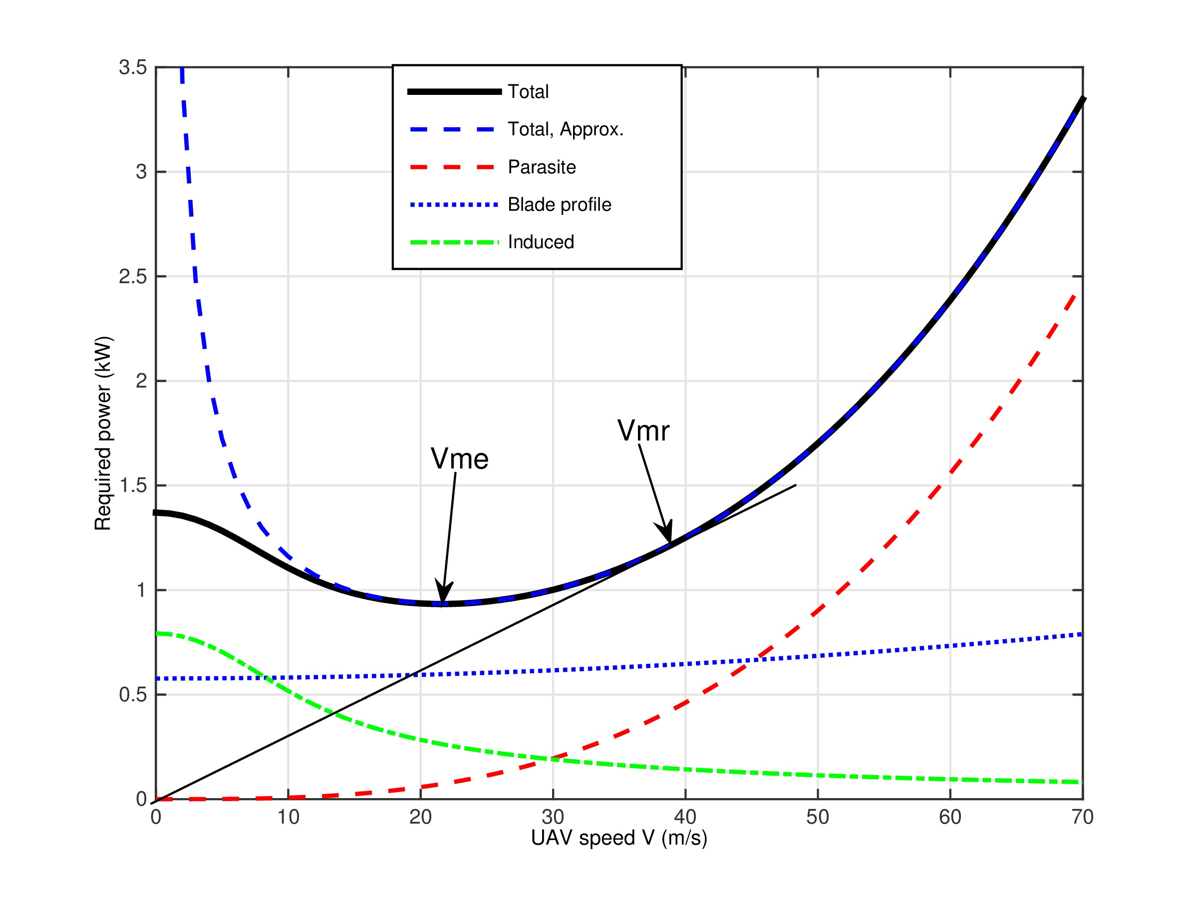
Figure 1: Propulsion power consumption versus speed $V$ for rotary-wing UAV.

Two particular UAV speeds that are of high practical interests are the maximum-endurance (ME) speed and the maximum-range (MR) speed, which are denoted as $V_{\mathrm{me}}$ and $V_{\mathrm{mr}}$, respectively.

ME speed: By definition, the ME speed $V_{\mathrm{me}}$ is the optimal UAV speed that maximizes the UAV endurance under any given onboard energy $E$. With $E$ given, the UAV endurance with constant speed $V$ is given by $\frac{E}{P(V)}$. Thus, $V_{\mathrm{me}}$ is the optimal UAV speed that minimizes the power consumption, i.e., $V_{\mathrm{me}}=\mathrm{arg}~{}\underset{V\geq 0}{\min}\ P(V)$ Though a closed-form expression for $V_{\mathrm{me}}$ is difficult to obtain due to the complicated expression of $P(V)$ in (6), it can be efficiently found numerically.

MR speed: On the other hand, the MR speed $V_{\mathrm{mr}}$ is the optimal UAV speed that maximizes the total traveling distance with any given onboard energy $E$. For any given $E$, the range with constant traveling speed $V$ can be expressed as $\frac{EV}{P(V)}$. Define the function

$$E_{0}(V)\triangleq\frac{P(V)}{V} =P_{0}\left(\frac{1}{V}+\frac{3V}{U_{\mathrm{tip}}^{2}}\right)+P_{i}\left(\sqrt{V^{-4}+\frac{1}{4v_{0}^{4}}}-\frac{1}{2v_{0}^{2}}\right)^{1/2}+\frac{1}{2}d_{0}\rho sAV^{2},$$ (8)

which physically represents the UAV energy consumption per unit travelling distance in Joule/meter (J/m) with speed $V$. Thus, $V_{\mathrm{mr}}$ can be found as $V_{\mathrm{mr}}=\mathrm{arg}~{}\underset{V\geq 0}{\min}\ E_{0}(V)$ Though a closed-form expression for $V_{\mathrm{mr}}$ is difficult to obtain, it can be efficiently found numerically. Alternatively, $V_{\mathrm{mr}}$ can also be obtained graphically based on the power-speed curve $P(V)$, by drawing the tangential line from the origin to the power curve that corresponds to the minimum slope (and hence power/speed ratio) [34], as illustrated in Fig. 1. In practice, we usually have $V_{\mathrm{me}}\leq V_{\mathrm{mr}}\leq V_{\max}$.

With given UAV trajectory $\{\mathbf{q}(t)\}$, the propulsion energy consumption can be expressed as

$$E_{1}(T_{t},\{\mathbf{q}(t)\})=\int_{0}^{T_{t}}P(\|\mathbf{v}(t)\|)dt,$$ (9)

where $\mathbf{v}(t)\triangleq\dot{\mathbf{q}}(t)$ is the UAV velocity and $\|\mathbf{v}(t)\|$ is the UAV speed at time instant $t$.

By combining both the communication related energy and the propulsion energy, the total UAV energy consumption can be expressed as

$$E(T_{t},\{\mathbf{q}(t)\},\{\lambda_{k}(t)\})=E_{1}(T_{t},\{\mathbf{q}(t)\})+P_{c}\int_{0}^{T_{t}}\left(\sum_{k=1}^{K}\lambda_{k}(t)\right)dt.$$ (10)

II-C Problem Formulation for UAV Energy Minimization

Our objective is to minimize the UAV total energy consumption, while satisfying the target communication throughput requirement for each of the $K$ GNs. The problem can be formulated as

$$\mathrm{(P1):} \underset{T_{t},\{\mathbf{q}(t)\},\{\lambda_{k}(t)\}}{\min}\ E(T_{t},\{\mathbf{q}(t)\},\{\lambda_{k}(t)\})$$

$$\mathrm{s.t.}\ \bar{R}_{k}(T_{t},\{\mathbf{q}(t)\},\{\lambda_{k}(t)\})\geq\tilde{Q}_{k},\ \forall k\in\mathcal{K},$$ (11)

$$\|\dot{\mathbf{q}}(t)\|\leq V_{\max},\ \forall t\in[0,T_{t}],$$ (12)

$$\mathbf{q}(0)=\mathbf{q}_{I},\ \mathbf{q}(T_{t})=\mathbf{q}_{F},$$ (13)

$$\lambda_{k}(t)\in\{0,1\},\ \forall k\in\mathcal{K},\ t\in[0,T_{t}],$$ (14)

$$\sum_{k=1}^{K}\lambda_{k}(t)\leq 1,\ \forall t\in[0,T_{t}],$$ (15)

where $\mathbf{q}_{I},\mathbf{q}_{F}\in\mathbb{R}^{2\times 1}$ represent the UAV’s initial and final locations projected onto the horizontal plane, respectively. Note that depending on practical application scenarios, the constraints on the initial/final UAV locations in (13) may or may not be present.

Problem $\mathrm{(P1)}$ requires optimizing the UAV trajectory $\{\mathbf{q}(t)\}$ and communication scheduling $\{\lambda_{k}(t)\}$, which are both continuous functions with respect to time $t$. Therefore, $\mathrm{(P1)}$ essentially involves infinite number of optimization variables. Furthermore, $\mathrm{(P1)}$ includes a complicated cost function for the UAV energy consumption, as well as non-convex constraints in (11) and binary constraints in (14). Therefore, $\mathrm{(P1)}$ is difficult to be directly solved. In Section III, we first consider the simple fly-hover-communicate protocol to make the problem more tractable, by which $\mathrm{(P1)}$ reduces to a problem with a finite number of optimization variables that only depends on the number of GNs $K$, instead of the (a priori unknown) mission completion time $T_{t}$. Then in Section IV, we propose a general solution to $\mathrm{(P1)}$ by utilizing the new path disretization technique to convert it into a discretized equivalent problem with a finite number of optimization variables, for which at least a locally optimal solution can be found via the SCA technique.

III Fly-Hover-Communicate Protocol

Fly-hover-communicate is a very intuitive protocol that is also easy to implement in practice. In this protocol, the UAV successively visits $K$ optimized hovering locations, each for one GN, and communicates with each GN only when it is hovering at the corresponding location. As a result, problem $\mathrm{(P1)}$ reduces to finding the optimal hovering locations and hovering (communication) time allocations for the $K$ GNs, as well as the optimal flying speed and path connecting these hovering locations. In the following, we first consider the special case with only one GN to draw useful insights, and then extend the study to the general case with multiple GNs.

III-A Optimal Fly-Hover-Communicate Scheme for One Single GN

For the special case with one single GN, the GN index $k$ is omitted for brevity. Without loss of generality, we assume that the GN is located at the origin with $\mathbf{w}=\mathbf{0}$, and the UAV’s initial horizontal location is $\mathbf{q}_{I}=[\bar{D},0]^{T}$. To illustrate the fundamental trade-off between hovering energy and flying energy minimization, we assume that there is no constraint on the UAV’s final location in this subsection, where the general case with such a constraint will be studied in Section III-B and Section IV. It is not difficult to see that under such a basic setup, the UAV should only fly along the line segment connecting $\mathbf{q}_{I}$ and the GN $\mathbf{w}$.

One extreme case of the fly-hover-communicate protocol is that the UAV simply hovers at the initial location $\mathbf{q}_{I}$ and communicates with the GN until the aggregated information bits reach the target value $\tilde{Q}$. However, when the initial horizontal distance $\bar{D}$ is large, such a strategy usually leads to a very low data rate and hence requires very long mission completion time $T_{t}$. This in turn leads to high UAV hovering and communication energy consumption. Alternatively, the UAV could fly closer to the GN and hover at a certain location with a shorter link distance to achieve a higher data rate. This strategy, though requiring additional energy for UAV traveling, reduces the time for data transmission (or hovering), and hence requires less energy for hovering and communication. Therefore, with the fly-hover-communicate protocol, in order to minimize the total UAV energy consumption, there must exist an optimal UAV hovering location that strikes an optimal balance between minimizing the traveling energy and hovering/communication energy.

Denote by $T_{\mathrm{tr}}$ the UAV traveling time before reaching the hovering location and by $V(t)$ the instantaneous traveling speed towards the GN. Thus, the total traveling distance is $D_{\mathrm{tr}}=\int_{0}^{T_{\mathrm{tr}}}V(t)dt$, where we should have $0\leq D_{\mathrm{tr}}\leq\bar{D}$. The total required energy consumption for traveling is

$$E_{\mathrm{tr}}(T_{\mathrm{tr}},\{V(t)\})=\int_{0}^{T_{\mathrm{tr}}}P(V(t))dt.$$ (16)

Furthermore, based on (2), the achievable data rate in bps when the UAV hovers at the point after traveling distance ${D}_{\mathrm{tr}}$ is

$$R(D_{\mathrm{tr}})=B\log_{2}\left(1+\frac{\gamma_{0}}{H^{2}+(\bar{D}-D_{\mathrm{tr}})^{2}}\right).$$ (17)

Thus, the required communication time (or equivalently the UAV hovering time $T_{\mathrm{hov}}$) to complete the transmission of $\tilde{Q}$ bits is

$$T_{\mathrm{hov}}=\frac{\tilde{Q}}{R(D_{\mathrm{tr}})}=\frac{Q}{\log_{2}\left(1+\frac{\gamma_{0}}{H^{2}+(\bar{D}-D_{\mathrm{tr}})^{2}}\right)},$$ (18)

where $Q\triangleq\tilde{Q}/B$ is the bandwidth-normalized throughput requirement in bits/Hz. Thus, the total required UAV hovering and communication energy consumption is

$$E_{\mathrm{hc}}(D_{\mathrm{tr}})=(P_{h}+P_{c})T_{\mathrm{hov}}=\frac{(P_{h}+P_{c})Q}{\log_{2}\left(1+\frac{\gamma_{0}}{H^{2}+(\bar{D}-D_{\mathrm{tr}})^{2}}\right)}.$$ (19)

Therefore, the total UAV energy consumption is

$$E_{\mathrm{tot}}(T_{\mathrm{tr}},\{V(t)\},D_{\mathrm{tr}})=E_{\mathrm{tr}}(T_{\mathrm{tr}},\{V(t)\})+E_{\mathrm{hc}}(D_{\mathrm{tr}}).$$ (20)

Thus, the energy minimization problem $\mathrm{(P1)}$ reduces to

$$\mathrm{(P2)}\ \underset{T_{\mathrm{tr}},\{V(t)\},D_{\mathrm{tr}}}{\min}\ E_{\mathrm{tot}}(T_{\mathrm{tr}},\{V(t)\},D_{\mathrm{tr}})$$

s.t. $$0\leq V(t)\leq V_{\max},\forall t\in[0,T_{\mathrm{tr}}],$$

$$\int_{0}^{T_{\mathrm{tr}}}V(t)dt=D_{\mathrm{tr}},$$

$$0\leq D_{\mathrm{tr}}\leq\bar{D}.$$ (21)

It is not difficult to see that with the fly-hover-communicate protocol, the scheduling variable $\lambda(t)$ in problem $\mathrm{(P1)}$ can be directly determined once the UAV traveling time $T_{\mathrm{tr}}$ and hovering time $T_{\mathrm{hov}}$ are obtained.

Lemma 1.

The optimal solution to problem $\mathrm{(P2)}$ satisfies $T_{\mathrm{tr}}=D_{\mathrm{tr}}/V_{\mathrm{mr}}$ and $V(t)=V_{\mathrm{mr}}$, $\forall t\in[0,D_{\mathrm{tr}}/V_{\mathrm{mr}}]$.

Proof:

Lemma 1 can be shown by change of variables. The details are omitted for brevity. ∎

Lemma 1 shows that with the fly-hover-communicate protocol, the UAV should travel with a constant speed, which is given by the MR speed, $V_{\mathrm{mr}}$. Let $E_{0}^{\star}=E_{0}(V_{\mathrm{mr}})$ be the minimum UAV energy consumption per unit traveling distance obtained by substituting $V_{\mathrm{mr}}$ into (8). Then problem $\mathrm{(P2)}$ reduces to the following uni-variate optimization problem

$$\underset{0\leq D_{\mathrm{tr}}\leq\bar{D}}{\min}\ D_{\mathrm{tr}}E_{0}^{\star}+\frac{(P_{h}+P_{c})Q}{\log_{2}\left(1+\frac{\gamma_{0}}{H^{2}+(\bar{D}-D_{\mathrm{tr}})^{2}}\right)}.$$ (22)

Note that the first term of (22) increases linearly with the traveling distance $D_{\mathrm{tr}}$, while the second term decreases monotonically with $D_{\mathrm{tr}}$. Therefore, the optimal solution of $D_{\mathrm{tr}}$ to problem (22) should balance the energy consumption for traveling and hovering, which can be efficiently obtained via a one-dimensional search.

For the asymptotical case in the low-SNR regime, e.g., $\gamma_{0}\ll H^{2}$, by applying the approximation $\ln(1+x)\approx x$ for $|x|\ll 1$, the optimal solution to (22) can be obtained in closed-form as $D_{\mathrm{tr}}^{*}=\max\left\{0,\bar{D}-\frac{\gamma_{0}E_{0}^{\star}}{(2\ln 2)(P_{h}+P_{c})Q}\right\}$. Define $Q^{\prime}\triangleq\frac{\gamma_{0}E_{0}^{\star}}{(2\ln 2)(P_{h}+P_{c})\bar{D}}$. The above result shows that the UAV should move closer (i.e., $D_{\mathrm{tr}}^{*}>0$) to the GN for communication only when $Q>Q^{\prime}$. Otherwise, it should simply hover at the initial location $\mathbf{q}_{I}$ for communication. Furthermore, the larger the throughput requirement $Q$ is, the closer the UAV should move towards the GT for communication. As $Q$ gets sufficiently large, we have $D_{\mathrm{tr}}^{*}\rightarrow\bar{D}$, i.e., the UAV should hover on top of the GN for commutation.

III-B Fly-Hover-Communicate for Multiple GNs

In this subsection, the fly-hover-communicate protocol is extended to the general case with multiple GNs. In this case, $\mathrm{(P1)}$ reduces to finding the optimal set of $K$ hovering locations, each for communicating with one GN, as well as the traveling path and speed among these hovering locations.

Let $\tilde{\mathbf{q}}_{k}\in\mathbb{R}^{2\times 1}$ denote the horizontal coordinate of the UAV hovering location when it communicates with GN $k$. Based on (2), the instantaneous communication rate in bps can be written as

$$R_{k}(\tilde{\mathbf{q}}_{k})=B\log_{2}\left(1+\frac{\gamma_{0}}{H^{2}+\|\tilde{\mathbf{q}}_{k}-\mathbf{w}_{k}\|^{2}}\right).$$ (23)

As a result, the total required communication time (or the hovering time at location $\tilde{\mathbf{q}}_{k}$) to ensure the target throughput $\tilde{Q}_{k}$ is given by

$$T_{k}(\tilde{\mathbf{q}}_{k})=\frac{\tilde{Q}_{k}}{R_{k}(\tilde{\mathbf{q}}_{k})}=\frac{Q_{k}}{\log_{2}\left(1+\frac{\gamma_{0}}{H^{2}+\|\tilde{\mathbf{q}}_{k}-\mathbf{w}_{k}\|^{2}}\right)},$$ (24)

where $Q_{k}\triangleq\tilde{Q}_{k}/B$ is the normalized throughput requirement in bits/Hz. Thus, the total required hovering and communication energy at the $K$ locations is a function of $\{\tilde{\mathbf{q}}_{k}\}$, which can be expressed as

$$E_{\mathrm{hc}}(\{\tilde{\mathbf{q}}_{k}\}) =(P_{h}+P_{c})\sum_{k=1}^{K}T_{k}(\tilde{\mathbf{q}}_{k})=\sum_{k=1}^{K}\frac{(P_{h}+P_{c})Q_{k}}{\log_{2}\left(1+\frac{\gamma_{0}}{H^{2}+\|\tilde{\mathbf{q}}_{k}-\mathbf{w}_{k}\|^{2}}\right)}.$$ (25)

On the other hand, the total required traveling energy depends on the total traveling distance $D_{\mathrm{tr}}$ to visit all the $K$ hovering locations $\{\tilde{\mathbf{q}}_{k}\}$, as well as the traveling speed $V(t)$ among them. Similar to Lemma 1, it can be shown that with the fly-hover-communicate protocol, the UAV should always travel with the MR speed $V_{\mathrm{mr}}$. Furthermore, for any given set of hovering locations $\{\tilde{\mathbf{q}}_{k}\}$ and initial/final locations ${\mathbf{q}}_{I}$ and ${\mathbf{q}}_{F}$, the total traveling distance $D_{\mathrm{tr}}$ depends on the visiting order of all the $K$ locations, which can be represented by the permutation variables $\pi(k)\in\{1,\cdots,K\}$. Specifically, $\pi(k)$ gives the index of the $k$th GN served by the UAV. Therefore, we have

$$D_{\mathrm{tr}}\left(\{\tilde{\mathbf{q}}_{k}\},\{\pi(k)\}\right)=\sum_{k=0}^{K}\|\tilde{\mathbf{q}}_{\pi(k+1)}-\tilde{\mathbf{q}}_{\pi(k)}\|,$$ (26)

where for convenience, we have defined $\tilde{\mathbf{q}}_{\pi(0)}={\mathbf{q}}_{I}$ and $\tilde{\mathbf{q}}_{\pi(K+1)}={\mathbf{q}}_{F}$. Thus, the total required UAV traveling energy with the optimal traveling speed $V_{\mathrm{mr}}$ can be written as

$$E_{\mathrm{tr}}\left(\{\tilde{\mathbf{q}}_{k}\},\{\pi(k)\}\right)=E_{0}^{\star}D_{\mathrm{tr}}\left(\{\tilde{\mathbf{q}}_{k}\},\{\pi(k)\}\right).$$ (27)

The total UAV energy consumption is thus given by

$$E_{\mathrm{tot}}\left(\{\tilde{\mathbf{q}}_{k}\},\{\pi(k)\}\right)=E_{\mathrm{hc}}(\{\tilde{\mathbf{q}}_{k}\})+E_{\mathrm{tr}}\left(\{\tilde{\mathbf{q}}_{k}\},\{\pi(k)\}\right).$$ (28)

As a result, the energy minimization problem $\mathrm{(P1)}$ with the fly-hover-communicate protocol reduces to

$$\mathrm{(P3)}:\ \underset{\{\tilde{\mathbf{q}}_{k}\},\{\pi(k)\}}{\min} \ E_{\mathrm{tot}}\left(\{\tilde{\mathbf{q}}_{k}\},\{\pi(k)\}\right)$$

$$\text{s.t.}\ \big{[}\pi(1),\cdots,\pi(K)\big{]}\in\mathcal{P},$$ (29)

where $\mathcal{P}$ represents the set of all the $K!$ possible permutations for the $K$ GNs. Note that with the fly-hover-communicate protocol, the user scheduling parameter $\{\lambda_{k}(t)\}$ in (P1) can be directly obtained based on the solution to $\mathrm{(P3)}$.

Problem $\mathrm{(P3)}$ is a non-convex optimization problem, whose optimal solution is difficult to obtain. In fact, even with fixed hovering locations $\{\tilde{\mathbf{q}}_{k}\}$, problem $\mathrm{(P3)}$ reduces to the classic TSP [35] with pre-determined initial and final locations [28], which is known to be NP hard. Therefore, problem $\mathrm{(P3)}$ is also NP hard as it is more general. Fortunately, by utilizing the existing techniques for solving TSP and applying convex optimization, an efficient approximate solution to $\mathrm{(P3)}$ can be obtained.

To this end, we first introduce the slack variables $D_{\mathrm{tr}}$ and $z_{k}=\|\tilde{\mathbf{q}}_{k}-\mathbf{w}_{k}\|^{2}$, by which problem $\mathrm{(P3)}$ can be equivalently written as

$$\mathrm{(P3.1)}: \underset{D_{\mathrm{tr}},\{\tilde{\mathbf{q}}_{k}\},\{\pi(k)\},\{z_{k}\}}{\min}\ E_{0}^{\star}D_{\mathrm{tr}}+\sum_{k=1}^{K}\frac{(P_{h}+P_{c})Q_{k}}{\log_{2}\left(1+\frac{\gamma_{0}}{H^{2}+z_{k}}\right)}$$

s.t. $$\big{[}\pi(1),\cdots,\pi(K)\big{]}\in\mathcal{P},$$ (30)

$$\sum_{k=0}^{K}\|\tilde{\mathbf{q}}_{\pi(k+1)}-\tilde{\mathbf{q}}_{\pi(k)}\|\leq D_{\mathrm{tr}},$$ (31)

$$\|\tilde{\mathbf{q}}_{k}-\mathbf{w}_{k}\|^{2}\leq z_{k},\ \forall k\in\mathcal{K}.$$ (32)

Note that at the optimal solution to $\mathrm{(P3.1)}$, all the constraints in (31) and (32) must be satisfied with strict equality, since otherwise, we may reduce $D_{\mathrm{tr}}$ or $z_{k}$ to further reduce the cost function of $\mathrm{(P3.1)}$.

Problem $\mathrm{(P3.1)}$ can be interpreted as follows. For each GN $k$, constraint (32) specifies a disk region centered at the GN location $\mathbf{w}_{k}$ with radius $\sqrt{z_{k}}$. The smaller $z_{k}$ is, the shorter the communication link distance between the UAV and GN $k$, and hence the less hovering-and-communication energy required (the second term of the cost function in $\mathrm{(P3.1)}$). However, due to constraint (31), this would generally require longer traveling distance $D_{\mathrm{tr}}$ and hence more traveling energy. In fact, for any fixed $\{z_{k}\}$ such that the hovering-and-communication energy is fixed, problem $\mathrm{(P3.1)}$ essentially reduces to minimizing the total traveling distance $D_{\mathrm{tr}}$, while ensuring that each of the hovering location $\tilde{\mathbf{q}}_{k}$ has a distance no greater than $\sqrt{z_{k}}$ from the GN $k$. This is essentially the classical traveling salesman problem with neighborhood (TSPN), with pre-determined initial and final locations. TSPN is a generalization of the TSP and hence is NP hard as well, where both the visiting order $\{\pi(k)\}$ and the locations $\{\tilde{\mathbf{q}}_{k}\}$ inside the disk region need to be optimized. One effective method for solving TSPN is to firstly ignore the disk radius and solve the TSP problem over the $K$ GN locations $\{\mathbf{w}_{k}\}$ to obtain the visiting order $[\hat{\pi}(1),\cdots,\hat{\pi}(K)]$ [28]. Though NP hard, TSP can be approximately solved with high-quality solutions by many existing algorithms [36]. As such, the TSPN then reduces to finding the optimal waypoints $\{\tilde{\mathbf{q}}_{k}\}$ with the obtained order $\{\hat{\pi}_{k}\}$, which is a convex optimization problem and hence can be optimally solved [28].

With the above idea, an efficient algorithm is proposed to solve problem $\mathrm{(P3.1)}$. Specifically, the visiting order $\{\pi(k)\}$ is firstly set as $\{\hat{\pi}(k)\}$ obtained by solving the TSP over the GNs’ locations $\{\mathbf{w}_{k}\}$. As such, problem $\mathrm{(P3.1)}$ reduces to

$$\mathrm{(P3.2)}: \underset{D_{\mathrm{tr}},\{\tilde{\mathbf{q}}_{k}\},\{z_{k}\},\{\eta_{k}\}}{\min}\ E_{0}^{\star}D_{\mathrm{tr}}+\sum_{k=1}^{K}\frac{(P_{h}+P_{c})Q_{k}}{\eta_{k}}$$

s.t. $$\sum_{k=0}^{K}\|\tilde{\mathbf{q}}_{\hat{\pi}(k+1)}-\tilde{\mathbf{q}}_{\hat{\pi}(k)}\|\leq D_{\mathrm{tr}},$$ (33)

$$\|\tilde{\mathbf{q}}_{k}-\mathbf{w}_{k}\|^{2}\leq z_{k},\ \forall k\in\mathcal{K}$$ (34)

$$\eta_{k}\geq 0,\ \forall k\in\mathcal{K},$$ (35)

$$\eta_{k}\leq\log_{2}\left(1+\frac{\gamma_{0}}{H^{2}+z_{k}}\right),\ \forall k\in\mathcal{K},$$ (36)

where we have introduced the slack variables $\{\eta_{k}\}$. It is noted that the cost function of $\mathrm{(P3.2)}$ and constraints (33)–(35) are all convex. However, the newly introduced constraint (36) is non-convex. Fortunately, as the right hand side (RHS) of (36) is a convex function, a global lower bound can be obtained based on the first-order Taylor approximation at the local point $z_{k}^{(l)}$, with the superscript $(l)$ denoting the $l$th iteration:

$$\log_{2}\left(1+\frac{\gamma_{0}}{H^{2}+z_{k}}\right)\geq\log_{2}\left(1+\frac{\gamma_{0}}{H^{2}+z_{k}^{(l)}}\right)+\rho_{k}(z_{k}-z_{k}^{(l)}),$$ (37)

where $\rho_{k}=\frac{-\gamma_{0}\log_{2}(e)}{(H^{2}+z_{k}^{(l)})(H^{2}+z_{k}^{(l)}+\gamma_{0})}$.

By replacing the RHS of (36) with its lower bound, we have the following problem:

$$\mathrm{(P3.3)}: \underset{D_{\mathrm{tr}},\{\tilde{\mathbf{q}}_{k}\},\{z_{k}\},\{\eta_{k}\}}{\min}\ E_{0}^{\star}D_{\mathrm{tr}}+\sum_{k=1}^{K}\frac{(P_{h}+P_{c})Q_{k}}{\eta_{k}}$$

$$\mathrm{s.t.}\ \eqref{eq:Constr4}-\eqref{eq:etakPositive},$$

$$\eta_{k}\leq\log_{2}\left(1+\frac{\gamma_{0}}{H^{2}+z_{k}^{(l)}}\right)+\rho_{k}(z_{k}-z_{k}^{(l)}),\ \forall k\in\mathcal{K}.$$ (38)

It can be verified that problem $\mathrm{(P3.3)}$ is convex, which can thus be efficiently solved by existing convex optimization toolbox such as CVX [39]. Furthermore, due to the global lower bound in (37), the optimal value of $\mathrm{(P3.3)}$ provides an upper bound to that of $\mathrm{(P3.2)}$. By successively updating the local point $\{z_{k}^{(l)}\}$, the SCA-based algorithm for solving $\mathrm{(P3.2)}$ is summarized in Algorithm 1.

Algorithm 1 SCA-based algorithm for Solving $\mathrm{(P3.2)}$.

1:  Initialization: set the initial hovering locations $\{\tilde{\mathbf{q}}_{k}^{(0)}\}$ and let $z_{k}^{(0)}=\|\tilde{\mathbf{q}}_{k}^{(0)}-\mathbf{w}_{k}\|$, $\forall k\in\mathcal{K}$. Let $l=0$.

2:  repeat

3:     Solve the convex problem $\mathrm{(P3.2)}$ and denote the optimal solution as $D_{\mathrm{tr}}^{*},\{\tilde{\mathbf{q}}_{k}^{*}\},\{z_{k}^{*}\}$, $\{\eta_{k}^{*}\}$.

4:     Update the local point as $z_{k}^{(l+1)}=z_{k}^{*},\forall k\in\mathcal{K}$.

5:     Update $l=l+1$.

6:  until the fractional decrease of the objective value of $\mathrm{(P3.2)}$ is below a given threshold $\epsilon$.

By following similar arguments as in [25] and [40], it can be shown that Algorithm 1 is guaranteed to converge to at least a locally optimal solution to problem $\mathrm{(P3.2)}$ that satisfies the KKT conditions.

IV General Solution to $\mathrm{(P1)}$ with Path Discretization and SCA

The fly-hover-communicate protocol in the preceding section gives an efficient solution to $\mathrm{(P1)}$, where the number of optimization variables only depends on $K$, rather than the mission completion time $T_{t}$. However, this protocol is strictly sub-optimal since the UAV does not communicate while flying. In this section, we propose a general solution to $\mathrm{(P1)}$ without this assumption via jointly optimizing the UAV trajectory and communication time allocation.

IV-A Path Discretization

Problem $\mathrm{(P1)}$ essentially involves an infinite number of optimization variables coupled in time-continues functions $\mathbf{q}(t)$ and $\lambda_{k}(t)$, as well as the unknown mission completion time $T_{t}$, thus making it difficult to be directly solved. To obtain a more tractable form with a finite number of optimization variables, $\mathrm{(P1)}$ can be reformulated by disretizing the variables $\{\mathbf{q}(t)\}$ and $\{\lambda_{k}(t)\}$. To this end, prior works such as [23] and [25] mostly adopted the method of time discretization, where the time horizon $[0,T_{t}]$ is discretized into a finite number of time slots with sufficiently small slot length $\delta_{t}$. However, this method requires that the UAV mission completion time $T_{t}$ to be pre-specified, which is not the case for our considered energy minimization problem with $T_{t}$ being an optimization variable as well. One method to address the above issue is by firstly assuming a certain operation time $T_{t}$, based on which the time discretization method is applied to solve the corresponding optimization problem, and then exhaustively search for the optimal $T_{t}$. However, this would require to solve a prohibitively large number of optimization problems, each for a given assumed $T_{t}$, thus making it impractical especially when the optimal $T_{t}$ is moderately large. To address this issue, in the following, we propose an alternative discretization method, called path discretization, with which only one optimization problem needs to be solved.

We first clarify the terminologies of trajectory versus path. Generally, a path specifies the route that the UAV follows, i.e., all locations along the UAV trajectory, and it does not involve the time dimension. On the other hand, a trajectory includes its path together with the instantaneous travelling speed along the path, and thus it involves the time dimension. With path discretization, the UAV path (instead of time) is discretized into $M+1$ line segments, which are represented by $M+2$ waypoints $\{\mathbf{q}_{m}\}_{m=0}^{M+1}$, with $\mathbf{q}_{0}=\mathbf{q}_{I}$ and $\mathbf{q}_{M+1}=\mathbf{q}_{F}$. We impose the following constraints:

$$\|\mathbf{q}_{m+1}-\mathbf{q}_{m}\|\leq\Delta_{\max},\ \forall m,$$ (39)

where $\Delta_{\max}$ is an appropriately chosen value so that within each line segment, the UAV is assumed to fly with a constant velocity and the distance between the UAV and each GN is approximately unchanged. For instance, $\Delta_{\max}$ could be chosen such that $\Delta_{\max}\ll H$. Let $T_{m}$ denote the duration that the UAV remains in the $m$th line segment. The UAV flying velocity along the $m$th line segment is thus given by $\mathbf{v}_{m}=\frac{\mathbf{q}_{m+1}-\mathbf{q}_{m}}{T_{m}},\ \forall m$. Furthermore, the total mission completion time $T_{t}$ is given by $T_{t}=\sum_{m=0}^{M}T_{m}$.

As a result, with path discretization, the UAV trajectory $\{\mathbf{q}(t)\}$ is represented by the $M+2$ waypoints $\{\mathbf{q}_{m}\}_{m=0}^{M+1}$, together with the duration $\{T_{m}\}_{m=0}^{M}$ representing the time that the UAV spends within each line segment. With the given $\Delta_{\max}$, $M$ is chosen to be sufficiently large so that $(M+1)\Delta_{\max}\geq\hat{D}$, where $\hat{D}$ is an upper bound of the required total UAV flying distance. With such a discretization approach, there is no need to specify the mission completion time $T_{t}$ in advance, since it can be directly determined once $\{T_{m}\}$ are obtained. In addition, to characterize the special hovering status, path discretization only requires two discretization points, i.e., by simply letting $\mathbf{q}_{m}=\mathbf{q}_{m+1}$, regardless of the hovering duration $T_{m}$. This is in a sharp contrast to the existing time discretization approach, where the number of discretization points needs to increase linearly with $T_{m}$, even when the UAV is hovering and its location remains unchanged.

As such, the distance between the UAV and each GN $k$ can be written as

$$d_{mk}=\sqrt{H^{2}+\|\mathbf{q}_{m}-\mathbf{w}_{k}\|^{2}},\forall k,m,$$ (40)

where $d_{mk}$ represents the distance between the UAV and GN $k$ when the UAV is at the $m$th line segment along its path. As a result, the corresponding achievable rate expression in (2) for GN $k$ when the UAV is at the $m$th line segment can be represented as

$$R_{mk}=B\log_{2}\left(1+\frac{\gamma_{0}}{H^{2}+\|\mathbf{q}_{m}-\mathbf{w}_{k}\|^{2}}\right).$$ (41)

Furthermore, for each line segment $m$ along the UAV path, with TDMA among the $K$ GNs, let $\tau_{mk}\geq 0$ denote the allocated time for the UAV to communicate with GN $k$. Then constraint (3) can be written as $\sum_{k=1}^{K}\tau_{mk}\leq T_{m},\ \forall m\in\{0,\cdots,M\}$.

The aggregated communication throughput for GN $k$ in (II-A) can be written as

$$\bar{R}_{k}(\{\mathbf{q}_{m}\},\{\tau_{mk}\})=B\sum_{m=0}^{M}\tau_{mk}\log_{2}\left(1+\frac{\gamma_{0}}{H^{2}+\|\mathbf{q}_{m}-\mathbf{w}_{k}\|^{2}}\right).$$ (42)

Furthermore, the UAV energy consumption in (10) can be written as

$$E (\{T_{m}\},\{\mathbf{q}_{m}\},\{\tau_{mk}\})=\sum_{m=0}^{M}T_{m}P\left(\frac{\Delta_{m}}{T_{m}}\right)+P_{c}\sum_{m=0}^{M}\sum_{k=1}^{K}\tau_{mk}$$ (43)

$$=P_{0}\sum_{m=0}^{M}\left(T_{m}+\frac{3\Delta_{m}^{2}}{U_{\mathrm{tip}}^{2}T_{m}}\right)+P_{i}\sum_{m=0}^{M}\left(\sqrt{T_{m}^{4}+\frac{\Delta_{m}^{4}}{4v_{0}^{4}}}-\frac{\Delta_{m}^{2}}{2v_{0}^{2}}\right)^{1/2}+\frac{1}{2}d_{0}\rho sA\sum_{m=0}^{M}\frac{\Delta_{m}^{3}}{T_{m}^{2}}+P_{c}\sum_{m=0}^{M}\sum_{k=1}^{K}\tau_{mk},$$

where $\Delta_{m}\triangleq\|\mathbf{q}_{m+1}-\mathbf{q}_{m}\|$ is the length of the $m$th line segment. Note that in (43), we have used the expression (6) and the fact that the UAV speed at the $m$th line segment is $\|\mathbf{v}_{m}\|=\Delta_{m}/T_{m}$.

As a result, the energy minimization problem $\mathrm{(P1)}$ can be expressed in the discrete form as

$$\mathrm{(P4):} \underset{\{\mathbf{q}_{m}\},\{T_{m}\},\{\tau_{mk}\}}{\min}\ E(\{T_{m}\},\{\mathbf{q}_{m}\},\{\tau_{mk}\})$$

$$\mathrm{s.t.}\ \sum_{m=0}^{M}\tau_{mk}\log_{2}\left(1+\frac{\gamma_{0}}{H^{2}+\|\mathbf{q}_{m}-\mathbf{w}_{k}\|^{2}}\right)\geq Q_{k},\ \forall k,$$ (44)

$$\|\mathbf{q}_{m+1}-\mathbf{q}_{m}\|\leq\min\{\Delta_{\max},T_{m}V_{\max}\},\ \forall m\in\{1,\cdots,M\},$$ (45)

$$\mathbf{q}_{0}=\mathbf{q}_{I},\ \mathbf{q}_{M+1}=\mathbf{q}_{F},$$ (46)

$$\sum_{k=1}^{K}\tau_{mk}\leq T_{m},\ \forall m\in\{0,\cdots,M\},$$ (47)

$$\tau_{mk}\geq 0,\ \forall k\in\mathcal{K},m\in\{0,\cdots,M\}.$$ (48)

where (45) corresponds to the maximum UAV speed constraint as well as the maximum segment length constraint.

Notice that in problem $\mathrm{(P4)}$, the constraints (45)–(48) are all convex. However, both the cost function $E(\{T_{m}\},\{\mathbf{q}_{m}\},\{\tau_{mk}\})$ in (43) and the throughput constraint (44) are non-convex. Therefore, problem $\mathrm{(P4)}$ is non-convex and it is difficult to find its globally optimal solution. In the following, we propose an efficient algorithm to find (at least) a locally optimal solution to $\mathrm{(P4)}$ based on the SCA technique.

IV-B Proposed Solution to $\mathrm{(P4)}$

Firstly, we deal with the non-convex cost function of $\mathrm{(P4)}$. A closer look at the expression in (43) reveals that the first, third, and fourth terms are all convex functions with the respect to $\{\mathbf{q}_{m}\}$, $\{T_{m}\}$, and $\tau_{mk}$, which can be shown by using the fact that perspective operation preserves convexity [41]. However, the second term is non-convex. To tackle this issue, we introduce slack variables $\{y_{m}\geq 0\}$ such that

$$y_{m}^{2}=\sqrt{T_{m}^{4}+\frac{\Delta_{m}^{4}}{4v_{0}^{4}}}-\frac{\Delta_{m}^{2}}{2v_{0}^{2}},\ \forall m\in\{0,\cdots,M\},$$ (49)

which is equivalent to

$$\frac{T_{m}^{4}}{y_{m}^{2}}=y_{m}^{2}+\frac{\Delta_{m}^{2}}{v_{0}^{2}},\ \forall m\in\{0,\cdots,M\}.$$ (50)

Therefore, the second term of (43) can be replaced by the linear expression $P_{i}\sum_{m=0}^{M}y_{m}$, with the additional constraint (50).

On the other hand, to deal with the non-convex constraint (44), we introduce slack variables $\{A_{mk}\}$ such that

$$A_{mk}^{2}=\tau_{mk}\log_{2}\left(1+\frac{\gamma_{0}}{H^{2}+\|\mathbf{q}_{m}-\mathbf{w}_{k}\|^{2}}\right).$$ (51)

As a result, the constraint (44) can be equivalently written as $\sum_{m=0}^{M}A_{mk}^{2}\geq Q_{k},\ \forall k$. With the above manipulations, $\mathrm{(P4)}$ can be written as

$$\mathrm{(P4.1):} \underset{\begin{subarray}{c}\{\mathbf{q}_{m}\},\{T_{m}\},\{\tau_{mk}\}\\ \{y_{m}\},\{A_{mk}\}\end{subarray}}{\min}\ P_{0}\sum_{m=0}^{M}\left(T_{m}+\frac{3\Delta_{m}^{2}}{U_{\mathrm{tip}}^{2}T_{m}}\right)+P_{i}\sum_{m=0}^{M}y_{m}+\frac{1}{2}d_{0}\rho sA\sum_{m=0}^{M}\frac{\Delta_{m}^{3}}{T_{m}^{2}}+P_{c}\sum_{m=0}^{M}\sum_{k=1}^{K}\tau_{mk}$$

s.t. $$\sum_{m=0}^{M}A_{mk}^{2}\geq Q_{k},\ \forall k,$$ (52)

$$\frac{T_{m}^{4}}{y_{m}^{2}}\leq y_{m}^{2}+\frac{\|\mathbf{q}_{m+1}-\mathbf{q}_{m}\|^{2}}{v_{0}^{2}},\ \forall m,$$ (53)

$$\frac{A_{mk}^{2}}{\tau_{mk}}\leq\log_{2}\left(1+\frac{\gamma_{0}}{H^{2}+\|\mathbf{q}_{m}-\mathbf{w}_{k}\|^{2}}\right),\ \forall m,k,$$ (54)

$$y_{m}\geq 0,\forall m,$$ (55)

$$\eqref{eq:maxSpeedConstr}\text{--}\eqref{eq:tauConstr}.$$

Note that in $\mathrm{(P4.1)}$, the constraints (53) and (54) are obtained from (50) and (51) by replacing the equality sign with inequality constraints. This does not affect the equivalence between problem $\mathrm{(P4)}$ and $\mathrm{(P4.1)}$. To see this, suppose that at the optimal solution to $\mathrm{(P4.1)}$, if any of the constraint in (53) is satisfied with strict inequality, then we may reduce the corresponding value of the slack variable $y_{m}$ to make the constraint (53) satisfied with strict equality, and at the same time reduce the cost function. Therefore, at the optimal solution to $\mathrm{(P4.1)}$, all constraints in (53) must be satisfied with equality. Similarly, there always exists an optimal solution to $\mathrm{(P4.1)}$ that makes all constraints in (54) satisfied with equality as well. Thus, problem $\mathrm{(P4)}$ and $\mathrm{(P4.1)}$ are equivalent.

Problem $\mathrm{(P4.1)}$ is still non-convex due to the non-convex constraints (52)–(54). However, all these three constraints can be effectively handled with the SCA technique by deriving the global lower bounds at a given local point. Specifically, for the constraint (52), it is noted that the left hand side (LHS) is a convex function with respect to $A_{mk}$. By using the fact that the first-order Taylor expansion is a global lower bound of a convex function, we have the following inequality

$$A_{mk}^{2}\geq{A}_{mk}^{(l)2}+2{A}_{mk}^{(l)}(A_{mk}-{A}_{mk}^{(l)}),$$ (56)

where ${A}_{mk}^{(l)}$ is the value of $A_{mk}$ at the $l$th iteration.

Similarly, for the non-convex constraint (53), the LHS is already a jointly convex function with respect to $y_{m}$ and $T_{m}$, and the RHS of the inequality constraint is also a convex function. By applying the first-order Taylor expansion of the RHS, the following global lower bound can be obtained as

$$y_{m}^{2} +\frac{\|\mathbf{q}_{m+1}-\mathbf{q}_{m}\|^{2}}{v_{0}^{2}}\geq y_{m}^{(l)2}+2y_{m}^{(l)}(y_{m}-y_{m}^{(l)})-\frac{\|\mathbf{q}_{m+1}^{(l)}-\mathbf{q}_{m}^{(l)}\|^{2}}{v_{0}^{2}}+\frac{2}{v_{0}^{2}}(\mathbf{q}_{m+1}^{(l)}-\mathbf{q}_{m}^{(l)})^{T}(\mathbf{q}_{m+1}-\mathbf{q}_{m}),$$ (57)

where $y_{m}^{(l)}$ and $\mathbf{q}_{m}^{(l)}$ are the current value of the corresponding variables at the $l$th iteration.

Furthermore, for the non-convex constraint (54), the LHS is already a jointly convex function with respect to $A_{mk}$ and $\tau_{mk}$. In addition, with similar derivation as in [23] and [25], for any given value $\{{\mathbf{q}}_{m}^{(l)}\}$ at the $l$th iteration, a global concave lower bound can be obtained for the RHS of (54) as

$$\log_{2}\left(1+\frac{\gamma_{0}}{H^{2}+\|\mathbf{q}_{m}-\mathbf{w}_{k}\|^{2}}\right)\geq R_{mk}^{(l)}(\mathbf{q}_{m}),$$ (58)

where

$$R_{mk}^{(l)}(\mathbf{q}_{m})=\log_{2}\left(1+\frac{\gamma_{0}}{H^{2}+\|\mathbf{q}^{(l)}_{m}-\mathbf{w}_{k}\|^{2}}\right)-\beta_{mk}\left(\|\mathbf{q}_{m}-\mathbf{w}_{k}\|^{2}-\|{\mathbf{q}}^{(l)}_{m}-\mathbf{w}_{k}\|^{2}\right),$$ (59)

with $\beta_{mk}=\frac{(\log_{2}e)\gamma_{0}}{(H^{2}+\|{\mathbf{q}}^{(l)}_{m}-\mathbf{w}_{k}\|^{2})(\|{\mathbf{q}}^{(l)}_{m}-\mathbf{w}_{k}\|^{2}+\gamma_{0})}$.

By replacing the non-convex constraints (52)–(54) of $\mathrm{(P4.1)}$ with their corresponding lower bounds at the $l$th iteration obtained above, we have the following optimization problem:

$$\mathrm{(P4.2):} \underset{\begin{subarray}{c}\{\mathbf{q}_{m}\},\{T_{m}\},\{\tau_{mk}\}\\ \{y_{m}\},\{A_{mk}\}\end{subarray}}{\min}\ P_{0}\sum_{m=0}^{M}\left(T_{m}+\frac{3\Delta_{m}^{2}}{U_{\mathrm{tip}}^{2}T_{m}}\right)+P_{i}\sum_{m=0}^{M}y_{m}+\frac{1}{2}d_{0}\rho sA\sum_{m=0}^{M}\frac{\Delta_{m}^{3}}{T_{m}^{2}}+P_{c}\sum_{m=0}^{M}\sum_{k=1}^{K}\tau_{mk}$$

s.t. $$\sum_{m=0}^{M}\left({A}_{mk}^{(l)2}+2{A}_{mk}^{(l)}(A_{mk}-{A}_{mk}^{(l)})\right)\geq Q_{k},\ \forall k,$$

$$\frac{T_{m}^{4}}{y_{m}^{2}}\leq y_{m}^{(l)2}+2y_{m}^{(l)}(y_{m}-y_{m}^{(l)})-\frac{\|\mathbf{q}_{m+1}^{(l)}-\mathbf{q}_{m}^{(l)}\|^{2}}{v_{0}^{2}}+\frac{2}{v_{0}^{2}}(\mathbf{q}_{m+1}^{(l)}-\mathbf{q}_{m}^{(l)})^{T}(\mathbf{q}_{m+1}-\mathbf{q}_{m}),\ \forall m,$$

$$\frac{A_{mk}^{2}}{\tau_{mk}}\leq R_{mk}^{(l)}(\mathbf{q}_{m}),\ \forall m,k,$$

$$y_{m}\geq 0,\forall m,$$

$$\eqref{eq:maxSpeedConstr}\text{--}\eqref{eq:tauConstr}.$$

It can be verified that problem $\mathrm{(P4.2)}$ is a convex optimization problem, which can thus be efficiently solved by using standard convex optimization techniques or existing software toolbox such as CVX. Note that due to the global lower bounds in (56)–(58), if the constraints of problem $\mathrm{(P4.2)}$ are satisfied, then those for the original problem $\mathrm{(P4.1)}$ are guaranteed to be satisfied as well, but the reverse is not necessarily true. Thus, the feasible region of $\mathrm{(P4.2)}$ is in general a subset of that for $\mathrm{(P4.1)}$, and the optimal value of $\mathrm{(P4.2)}$ provides an upper bound to that of $\mathrm{(P4.1)}$. By successively updating the local point at each iteration via solving $\mathrm{(P4.2)}$, an efficient algorithm is obtained for the non-convex optimization problem $\mathrm{(P4.1)}$ or its original problem $\mathrm{(P4)}$. The algorithm is summarized as Algorithm 2.

Algorithm 2 SCA-based algorithm for $\mathrm{(P4)}$.

1:  Initialization: obtain a feasible $\{\mathbf{q}_{m}^{(0)}\}$, $\{T_{m}^{(0)}\}$, and $\{\tau_{mk}^{(0)}\}$ to $\mathrm{(P4)}$. Let $l=0$.

2:  repeat

3:     Calculate the current values $\{y_{m}^{(l)}\}$ and $\{A_{mk}^{(l)}\}$ based on (49) and (51), respectively.

4:     Solve the convex problem $\mathrm{(P4.2)}$, and denote the optimal solution as $\{\mathbf{q}_{m}^{*}\}$, $\{T_{m}^{*}\}$, $\{\tau_{mk}^{*}\}$.

5:     Update the local point $\mathbf{q}^{(l+1)}_{m}=\mathbf{q}_{m}^{*}$, $T_{m}^{(l+1)}=T_{m}^{*}$, and $\tau_{mk}^{(l+1)}=\tau_{mk}^{*}$.

6:     Update $l=l+1$.

7:  until the fractional decrease of the objective value of $\mathrm{(P4.2)}$ is below a given threshold $\epsilon$.

By following similar arguments as in [25] and [40], it can be shown that Algorithm 2 is guaranteed to converge to at least a locally optimal solution that satisfies the KKT conditions of problem $\mathrm{(P4.1)}$.

Remark 1.

While Algorithm 2 is proposed to minimize the UAV energy consumption, it can be similarly applied for UAV communication with other design metrics, such as the following mission completion time minimization problem, by replacing the cost function of $\mathrm{(P4)}$ with $\sum_{m=0}^{M}T_{m}$.

V Numerical Results

This section provides numerical results to validate the proposed designs. The UAV altitude is set as $H=100$ m and the total communication bandwidth is $B=1$ MHz. The received SNR at the reference distance of 1 m is $\gamma_{0}=60$ dB. As a result, the maximum received SNR when the UAV is just above each GN is $\gamma_{0}/H^{2}=20$ dB. The communication related power consumption at the UAV is fixed as $P_{c}=50$ W. For the UAV’s propulsion power consumption, the corresponding parameters are specified in Table I. The maximum flying speed is $V_{\max}=60$ m/s. The UAV’s initial and final locations are set as $\mathbf{q}_{I}=[0,0]^{T}$ and $\mathbf{q}_{F}=[800\text{ m},800\text{ m}]^{T}$, respectively. We consider the setup with $K=3$ GNs, with their locations shown in red squares in Fig. 3. We assume that all GNs have identical throughput requirements, i.e., $\tilde{Q}_{k}=\tilde{Q}$, $\forall k\in\mathcal{K}$.

First, we study the convergence of Algorithm 2 (Note that the convergence of Algorithm 1 can be shown similarly, for which the result is omitted due to the space limitation). The UAV initial path $\{\mathbf{q}_{m}^{(0)}\}$ is set as that obtained by the optimized fly-hover-communicate protocol proposed in Section III, and the initial duration $\{T_{m}^{(0)}\}$ at each line segment and communication time allocation $\{\tau_{mk}^{(0)}\}$ is obtained by letting $T_{m}^{(0)}=\bar{T}$, $\forall m$, and $\tau_{mk}^{(0)}=\bar{T}/K$, $\forall m,k$, where $\bar{T}$ is the minimum value that makes $\mathrm{(P4)}$ feasible. Fig. 2 shows the convergence of Algorithm 2 for throughput requirement $\tilde{Q}=200$ Mbits. The curve “Upper bound” corresponds to the obtained objective value of $\mathrm{(P4.2)}$, while “Exact” refers to the true UAV energy consumption value calculated based on (43). It is firstly observed that the two curves match quite well with each other, which demonstrates that the upper bound for UAV energy consumption via solving the convex optimization problem $\mathrm{(P4.2)}$ is practically tight. Furthermore, Fig. 2 shows that the proposed algorithm converges in a few iterations, which demonstrates the effectiveness of SCA for the proposed joint trajectory and communication time allocation design.

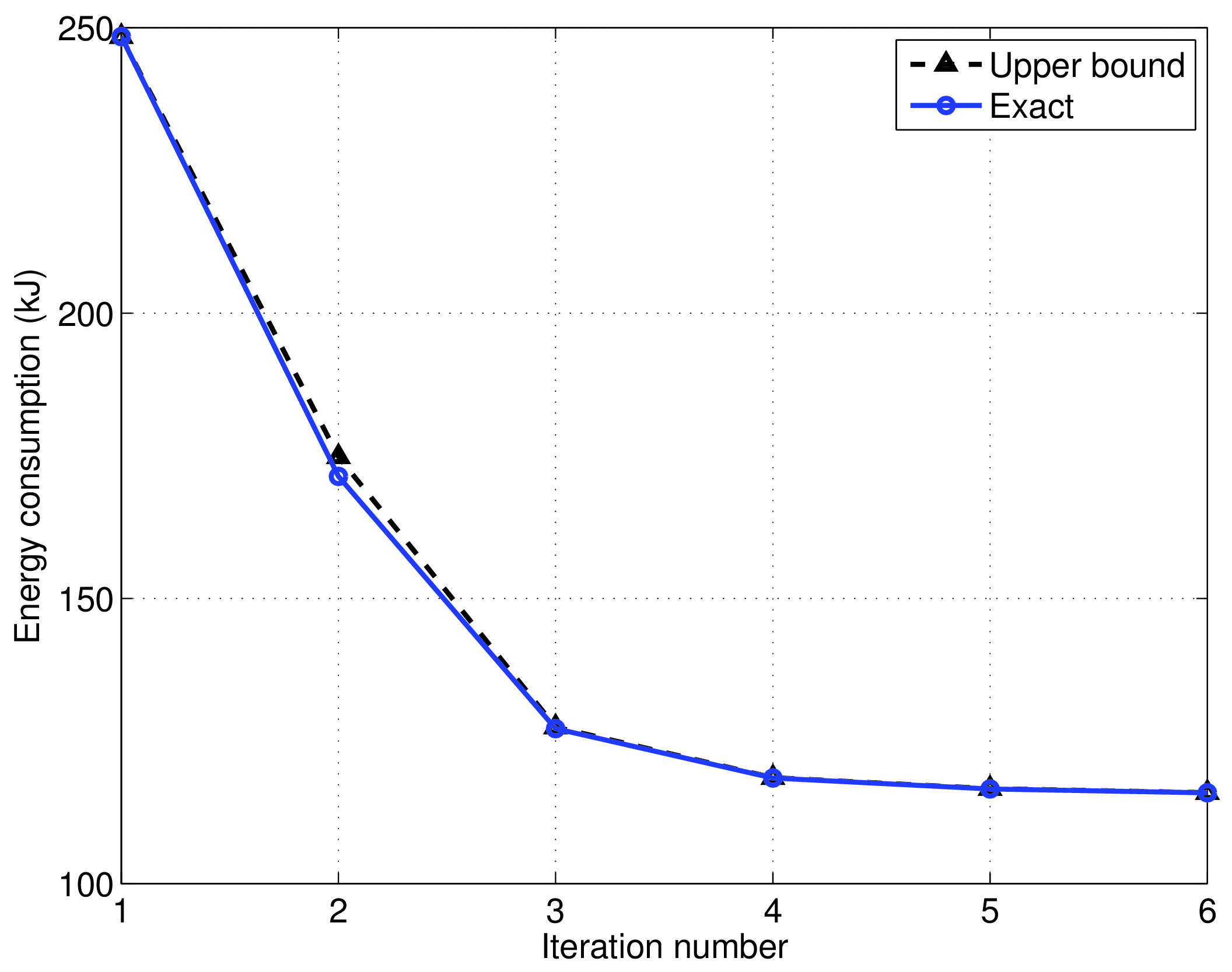
Figure 2: Convergence of Algorithm 2 for UAV energy minimization.

For $\tilde{Q}=50$ Mbits and $200$ Mbits, Fig. 3 and Fig. 4 respectively show the obtained UAV trajectories and the corresponding UAV speed with three different designs: i) Optimized fly-hover-communicate protocol proposed in Section III; ii) The SCA-based energy minimization design in Algorithm 2; and iii) The SCA-based time minimization design by similarly applying Algorithm 2. For the SCA-based energy minimization trajectory, Fig. 3 also shows the corresponding time instant when the UAV reaches the nearest position from each GN, for the convenience of illustrating the corresponding UAV speed shown in Fig. 4. It is firstly observed from Fig. 3 that for the proposed fly-hover-communicate protocol, the optimized hovering locations are in general different from the GN locations. This is expected due to the following trade-off: while hovering exactly above each GN achieves the minimal communication link distance and hence reduces the total communication time, it requires the UAV to travel longer distance and hence more energy consumption is needed for UAV flying. With the optimized fly-hover-communicate protocol, a balance between the above two conflicting objectives is achieved via optimizing the hovering locations for communication. By comparing Fig. 3(a) and Fig. 3(b), it is observed that the higher the throughput requirement is, the closer the optimized hovering locations will be from the GN locations, as expected. It is further observed from Fig. 4 that with the optimized fly-hover-communicate protocol, the UAV speed has only two status: flying with the MR speed $V_{\mathrm{mr}}$ between different optimized locations, or hovering above those locations for communicating with the corresponding GN.

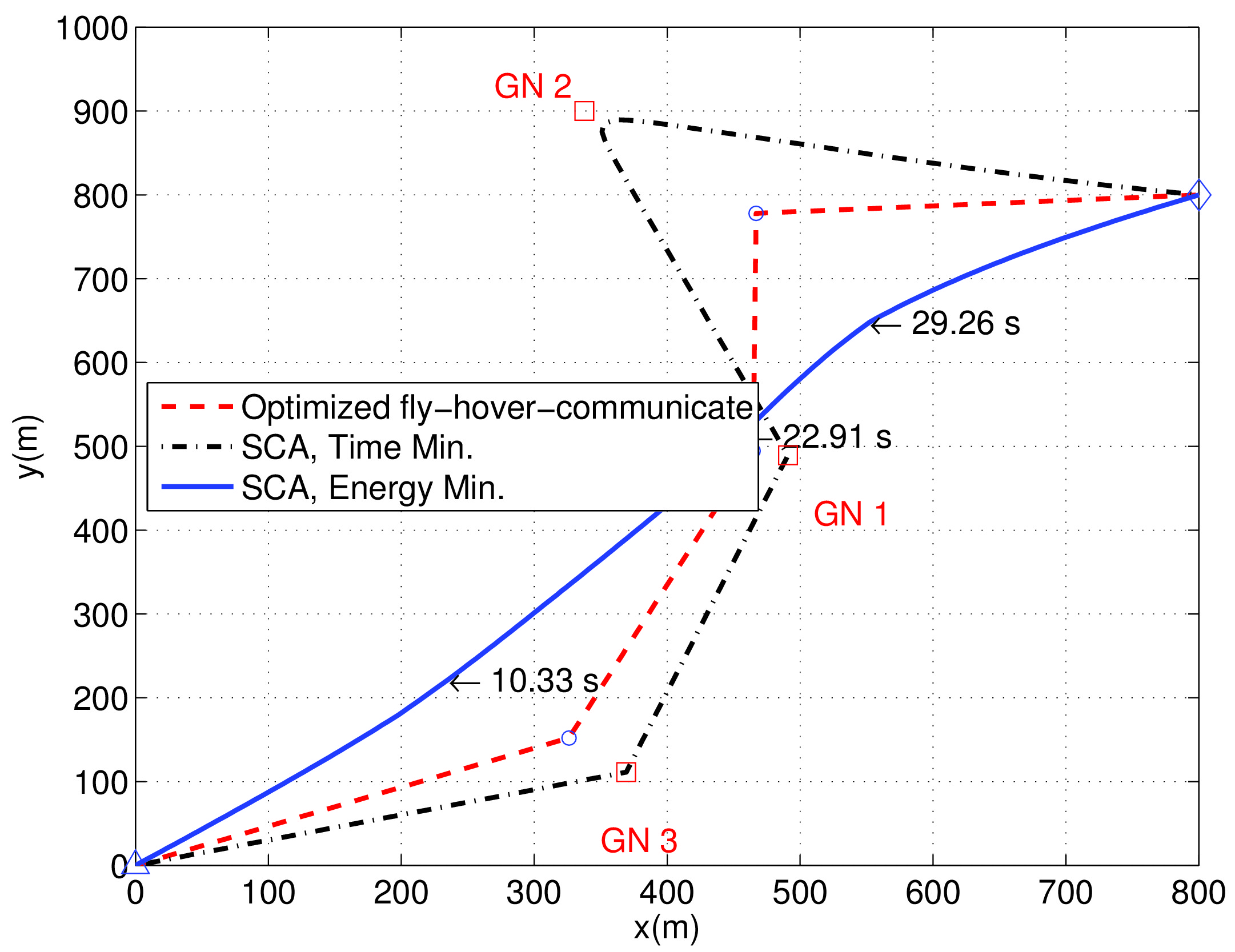
(a) $\tilde{Q}=50$ Mbits.

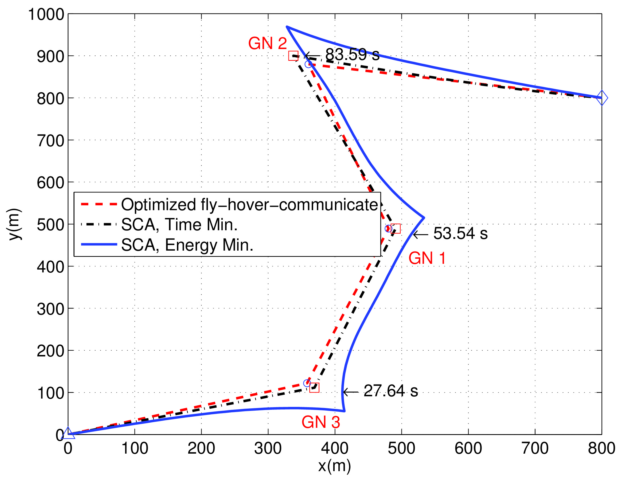
(b) $\tilde{Q}=200$ Mbits.

Figure 3: UAV trajectories with three different designs. Red squares denote GNs, and blue circles represent the optimized hovering locations in the fly-hover-communicate protocol.

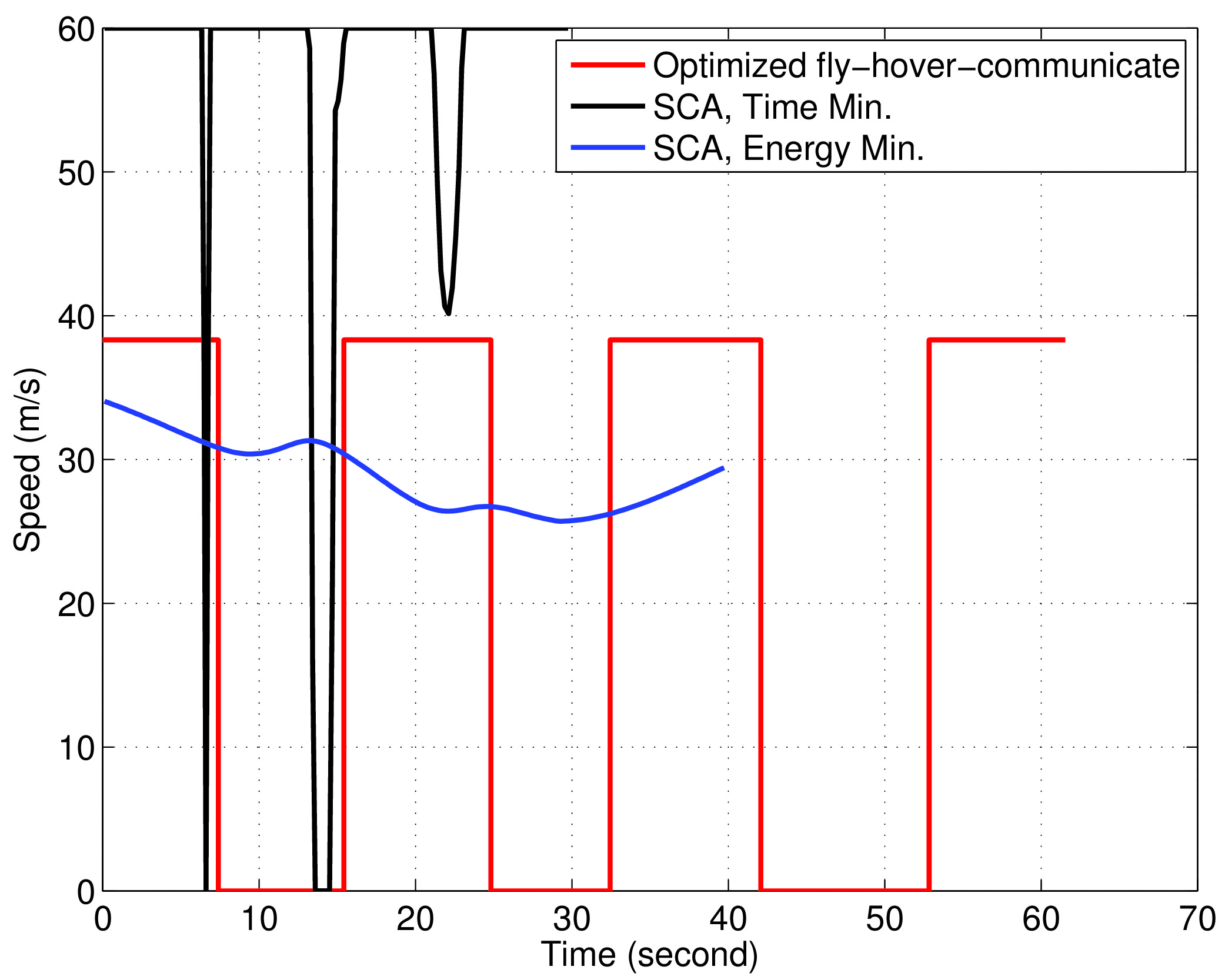
(a) $\tilde{Q}=50$ Mbits.

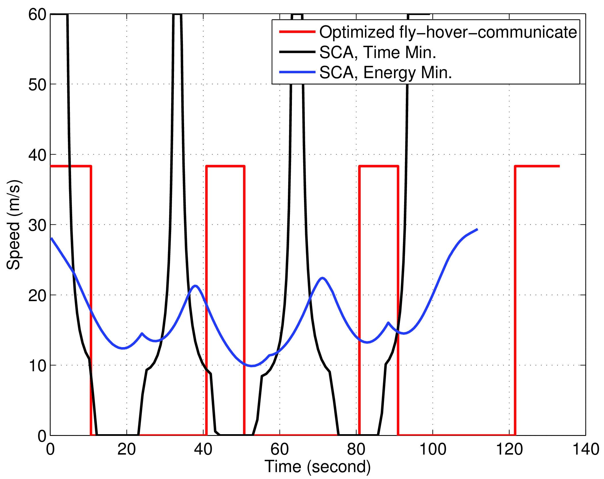
(b) $\tilde{Q}=200$ Mbits.

Figure 4: UAV speed versus time for different trajectories in Fig. 3.

For the proposed SCA-based algorithm for energy minimization, it is found from Fig. 3 that for the case with relatively low throughput requirement of $\tilde{Q}=50$ Mbits, the resulting UAV trajectory is almost a straight flight from $\mathbf{q}_{I}$ to $\mathbf{q}_{F}$. By contrast, as $\tilde{Q}$ increases to $200$ Mbits, the UAV needs to deliberately detour its path towards the GNs. Interestingly, it is observed from Fig. 3(b) and Fig. 4(b) that as the UAV approaches the GN, it tends to keep flying around it with a certain speed, instead of hovering directly above it. This is due to the fact that hovering is not the most power-conserving UAV status, as shown in Fig. 1. Therefore, the UAV tends to maintain a certain speed in order to reduce power consumption, though this may make the UAV slightly further away from the GN (thus with smaller instantaneous communication rate). By combining Fig. 3 and Fig. 4, it is found that for the SCA-based trajectory for energy minimization, the UAV will reduce its flying speed when it is close to each GN, as expected.

With the SCA-based algorithm for time minimization, Fig. 3 shows that for both $\tilde{Q}=50$ Mbits and $\tilde{Q}=200$ Mbits, the UAV tends to fly to the top of each GN. This is expected since for time minimization without considering the UAV energy consumption, it is preferable for the UAV to fly at high speed so as to approach the GN as soon as possible to enjoy the favorable communication channel. This is verified by the speed plot in Fig. 4.

For the proposed SCA-based design for energy minimization with $\tilde{Q}=200$ Mbits, Fig. 5 shows the fraction of the allocated communication time among GNs at each time instant, namely the values of $\tau_{mk}/T_{m}$. By combining Fig. 3 and Fig. 5, it is found that at each UAV location, more communication time is allocated to the nearer GN, which is expected since allocating resources to better channels in general leads to higher spectrum efficiency.

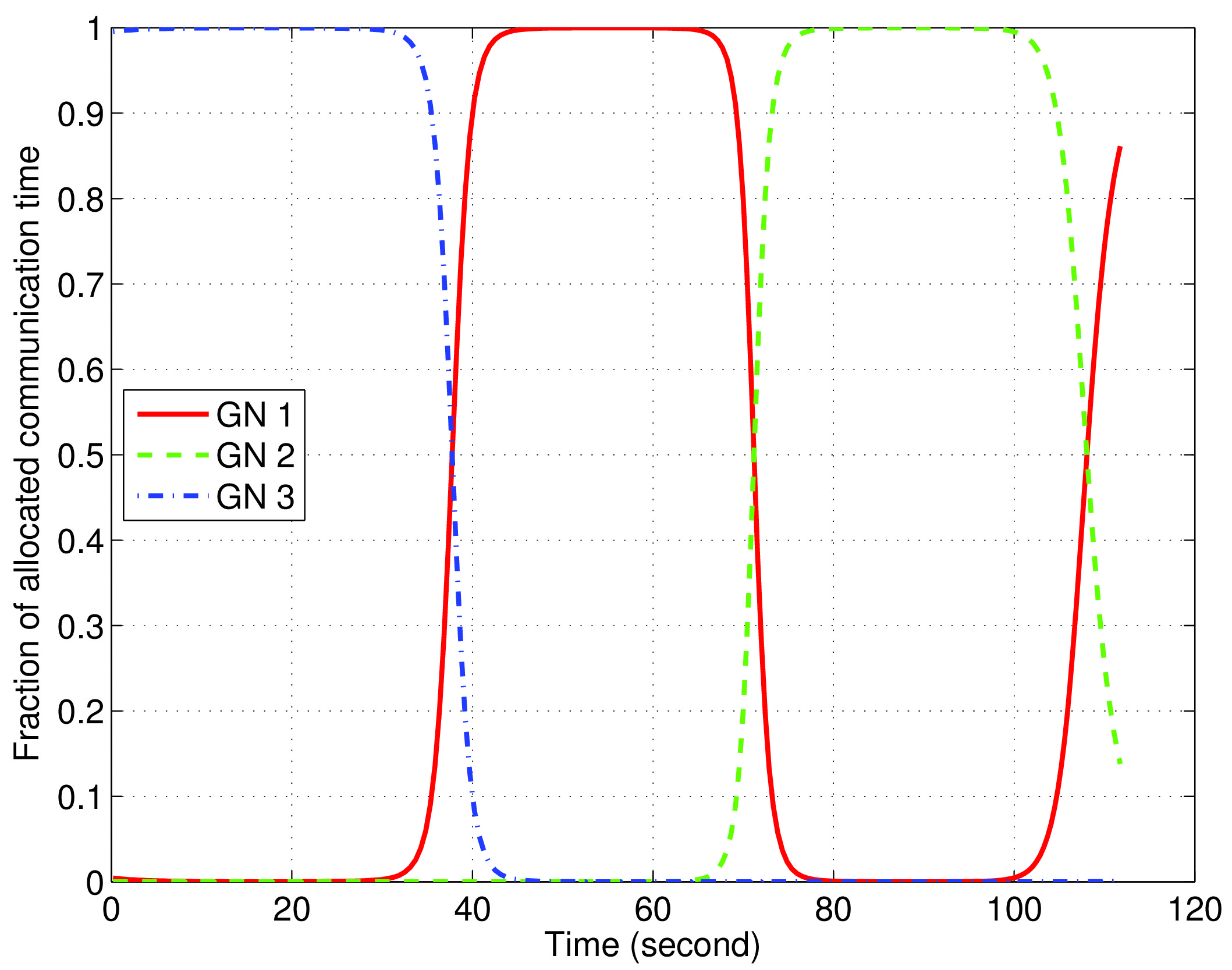
Figure 5: Fraction of allocated communicate time for SCA-based energy minimization.

Last, Fig. 6 shows the required UAV energy consumption and mission completion time versus the communication throughput requirement $\tilde{Q}$, respectively. Besides the three designs mentioned above, we also consider two alternative benchmark schemes, namely hovering at geometric center and hovering above GNs. Note that these two benchmark schemes correspond to the special cases of the general fly-hover-communicate protocol studied in Section III, where the hovering locations are fixed to either the geometric center of the $K$ GNs or each GN, instead of being optimized. It is firstly observed that in terms of both energy consumption and required mission completion time, “hovering at the geometric center” outperforms “hovering above GNs” for low throughput requirement, whereas the reverse is true as $\tilde{Q}$ increases. On the other hand, the optimized fly-hover-communicate scheme always outperforms both benchmark schemes, which is expected since it adaptively optimizes the hovering locations according to the communication requirement. Furthermore, with the proposed SCA algorithm either for energy minimization or time minimization, significant performance gains can be achieved. By comparing the two plots in Fig. 6, it is concluded that while minimizing the mission completion time can to certain extent help reduce the energy consumption and vice versa, the two design objectives in general lead to different solutions, and the explicit consideration of UAV energy consumption (instead of via the heuristic time minimization) results in further performance gains in terms of energy saving.

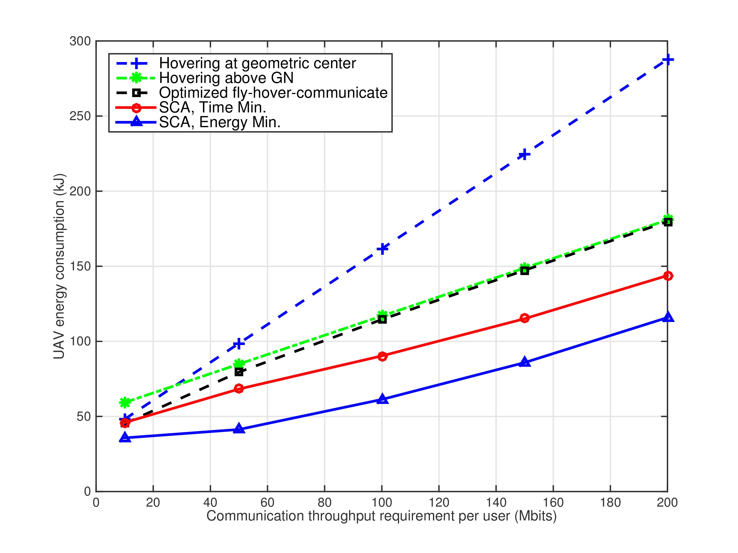
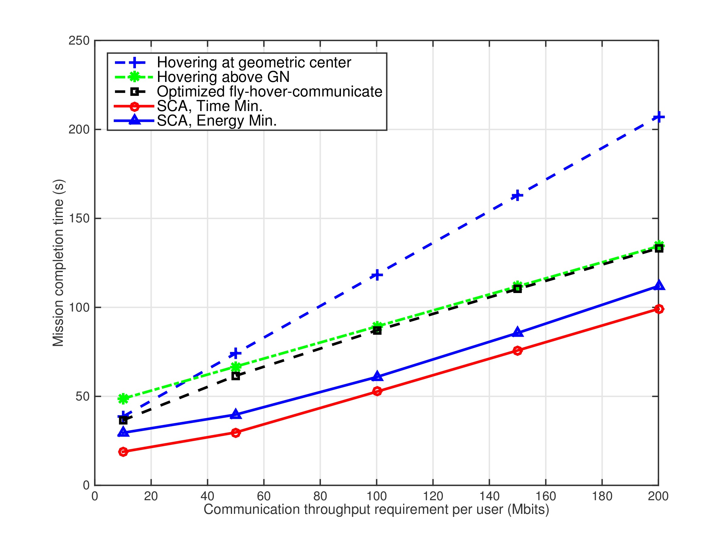
Figure 6: Energy consumption and mission completion time versus throughput requirement.

VI Conclusion

This paper studies the energy-efficient UAV communication with rotary-wing UAVs. The propulsion power consumption model of rotary-wing UAVs is derived, based on which an optimization problem is formulated to minimize the total UAV energy consumption, while satisfying the individual target communication throughput requirement for multiple GNs. We first propose an efficient solution based on the simple fly-hover-communicate protocol, which leverages the TSP and convex optimization techniques to find the optimized hovering locations and durations, as well as the visiting order and speed among these locations. Furthermore, we propose a general solution, with which the UAV communicates also when flying, by applying a new path discretization approach and the SCA technique. Numerical results show that the proposed designs achieve significant energy saving than other benchmark schemes for rotary-ring UAV enabled wireless communication systems.

Appendix A Power Consumption Model for Rotary-Wing UAVs

In this appendix, we derive the power consumption model for rotary-wing UAVs. Note that most of the notations and results follow from the textbook [33]. This appendix is NOT intended to introduce a new physical model for the power consumption of rotary-wing UAVs. Instead, it mainly aims to solicit the existing results in classic aircraft textbooks such as [33] and [34], to derive an analytical energy model that is suitable for research in UAV communications. Interested readers may refer to [33] and [34] for more detailed theoretical derivations based on actuator disc theory and blade element theory. The notations and terminologies used in this appendix are summarized in Table I.

TABLE I: Notations and terminologies for rotary-wing aircraft.

Notation	Physical meaning	Simulation value
$W$	Aircraft weight in Newton	$100$
$\rho$	Air density in kg/m3	$1.225$
$R$	Rotor radius in meter (m)	$0.5$
$A$	Rotor disc area in m2, $A\triangleq\pi R^{2}$	$0.79$
$\Omega$	Blade angular velocity in radians/second	$400$
$U_{\mathrm{tip}}$	Tip speed of the rotor blade, $U_{\mathrm{tip}}\triangleq\Omega R$	$200$
$b$	Number of blades	$4$
$c$	Blade or aerofoil chord length	$0.0196$
$s$	Rotor solidity, defined as the ratio of the total blade area $bcR$ to the disc area $A$, or $s\triangleq\frac{bc}{\pi R}$	$0.05$
$S_{FP}$	Fuselage equivalent flat plate area in $m^{2}$	$0.0118$
$d_{0}$	Fuselage drag ratio, defined as $d_{0}\triangleq\frac{S_{FP}}{sA}$	$0.3$
$k$	Incremental correction factor to induced power	$0.1$
$T$	Rotor thrust	–
$\kappa$	Thrust-to-weight ratio, $\kappa\triangleq\frac{T}{W}$	–
$t_{c}$	Thrust coefficient based on total blade area, defined as $t_{c}\triangleq\frac{T}{\rho sA\Omega^{2}R^{2}}$	–
$T_{D}$	Thrust component along the disc axes. $T_{D}\approx T$ in practice (Equation (1.39) of [33])	–
$t_{cD}$	Thrust coefficient referred to disc axes, $t_{cD}\triangleq\frac{T_{D}}{\rho sA\Omega^{2}R^{2}}\approx t_{c}$	–
$v_{0}$	Mean rotor induced velocity in hover, with $v_{0}=\sqrt{\frac{W}{2\rho A}}$ (see Equation (2.12) of [33] and Equation (12.1) of [34])	$7.2$
$v_{i0}$	Mean rotor induced velocity in forward flight	–
$\lambda_{i}$	Mean induced velocity normalized by tip speed, $\lambda_{i}\triangleq\frac{v_{i0}}{\Omega R}$	–
$\delta$	Profile drag coefficient.	$0.012$
$V$	Aircraft forward speed in m/s	–
$\hat{V}$	Forward speed normalized by tip speed, $\hat{V}\triangleq\frac{V}{\Omega R}$	–
$\alpha_{T}$	Tilt angle of the rotor disc, which is small in practice	–
$\mu$	Advance ratio, $\mu\approx\hat{V}=\frac{V}{\Omega R}$	–
$q_{c}$	Torque coefficient, which, by definition, is directly related to the required power $P$ as $P=q_{c}\rho sA\Omega^{3}R^{3}$. Note that in many text books, the required rotor power is usually given in terms of $q_{c}$.	–

For rotary-wing aircrafts in hovering status, the torque coefficient $q_{c}$ is given by Equation (2.45) of [33], i.e., $q_{c}=\frac{\delta}{8}+(1+k)\sqrt{\frac{s}{2}}t_{c}^{3/2}$. By substituting $t_{c}=\frac{T}{\rho sA\Omega^{2}R^{2}}$ and noting that the thrust $T$ balances the aircraft weight in hovering status, i.e., $T=W$, we have

$$q_{c}=\frac{\delta}{8}+(1+k)\frac{W^{3/2}}{\sqrt{2}\rho^{3/2}sA^{3/2}\Omega^{3}R^{3}}.$$ (60)

Therefore, by definition of the torque coefficient, the corresponding required power for hovering can be obtained based on the relationship $P=q_{c}\rho sA\Omega^{3}R^{3}$, which can be expressed as (see also Equation (12.13) of [34])

$$P_{h}=\underbrace{\frac{\delta}{8}\rho sA\Omega^{3}R^{3}}_{\triangleq P_{0}}+\underbrace{(1+k)\frac{W^{3/2}}{\sqrt{2\rho A}}}_{\triangleq P_{i}}.$$ (61)

The derivation of power required for forward flight of a rotary-wing aircraft is much more complicated than that of the fixed-wing counterpart [25]. Fortunately, under some mild assumptions, e.g., the drag coefficient of the blade section is constant, the torque coefficient $q_{c}$ for an aircraft in forward level flight (zero climbing angle) with speed $V$ is given by Equation (4.20) of [33], i.e.,

$$q_{c}=\frac{\delta}{8}(1+3\mu^{2})+(1+k)\lambda_{i}t_{cD}+\frac{1}{2}\hat{V}^{3}d_{0}.$$ (62)

By substituting with $\mu\approx\hat{V}=\frac{V}{\Omega R}$ and $t_{cD}=\frac{T}{\rho sA\Omega^{2}R^{2}}$, $q_{c}$ in (62) can be explicitly written as a function of the forward speed $V$ and rotor thrust $T$ as

$$q_{c}(V,T)=\frac{\delta}{8}\left(1+\frac{3V^{2}}{\Omega^{2}R^{2}}\right)+\frac{(1+k)T\lambda_{i}}{\rho sA\Omega^{2}R^{2}}+\frac{1}{2}d_{0}\frac{V^{3}}{\Omega^{3}R^{3}}.$$ (63)

By the definition of the torque coefficient, the required power can be written as a function of $V$ and $T$ as

$$P(V,T) \triangleq q_{c}(V,T)\rho sA\Omega^{3}R^{3}$$

$$=P_{0}\left(1+\frac{3V^{2}}{\Omega^{2}R^{2}}\right)+(1+k)Tv_{i0}+\frac{1}{2}d_{0}\rho sAV^{3},$$ (64)

where $v_{i0}=\lambda_{i}\Omega R$ is the mean induced velocity. Furthermore, based on Equation (3.2) of [33], for a rotary-wing aircraft with forward speed $V$ and rotor thrust $T$, the mean induced velocity can be calculated as

$$v_{i0} =\left(\sqrt{\frac{T^{2}}{4\rho^{2}A^{2}}+\frac{V^{4}}{4}}-\frac{V^{2}}{2}\right)^{1/2}=v_{0}\left(\sqrt{\kappa^{2}+\frac{V^{4}}{4v_{0}^{4}}}-\frac{V^{2}}{2v_{0}^{2}}\right)^{1/2},$$ (65)

where $v_{0}\triangleq\sqrt{\frac{W}{2\rho A}}$ is the mean induced velocity in hover and we have defined $\kappa$ as the thrust-to-weight ratio, i.e., $\kappa\triangleq\frac{T}{W}$. It can be shown that for any given thrust $T$ or $\kappa$, $v_{i0}$ is a decreasing function of $V$. By substituting (65) into (64), the required power for forward flight can be more explicitly written as

$$P(V,\kappa)= \underbrace{P_{0}\left(1+\frac{3V^{2}}{\Omega^{2}R^{2}}\right)}_{\text{blade profile}}+\underbrace{P_{i}\kappa\left(\sqrt{\kappa^{2}+\frac{V^{4}}{4v_{0}^{4}}}-\frac{V^{2}}{2v_{0}^{2}}\right)^{1/2}}_{\text{induced}}+\underbrace{\frac{1}{2}d_{0}\rho sAV^{3}}_{\text{parasite}},$$ (66)

where $P_{0}$ and $P_{i}$ are two constants defined in (61).

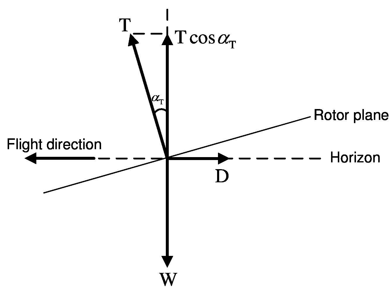
Figure 7: Schematics of the main forces acting on the aircraft in straight flight.

To obtain a more explicit expression of the required power in (66), we need to determine the rotor thrust $T$ or the thrust-to-weight ratio $\kappa$. Fig. 7 shows simplified schematics of the longitudinal forces acting on the aircraft in straight level flight (see also Figure 13.2 of [34]), which include the following forces: (i) $T$: rotor thrust, normal to the disc plane and directed upward; (ii) $D$: drag of fuselage, which is in the opposite direction of the aircraft velocity; and (iii) $W$: the aircraft weight. Due to the balance of forces in vertical direction, we have $T\cos\alpha_{T}=W$, where $\alpha_{T}$ is the tilt angle of the rotor disc. Note that in practice, $\alpha_{T}$ is usually very small, so we have $T\approx W$ or $\kappa\approx 1$ (see also Equation (4.3) of [33]). As a result, the expression in (66) reduces to (6) shown in Section II-B.

References

- [1] S. Chandrasekharan et al., “Designing and implementing future aerial communication networks,” IEEE Commun. Mag., vol. 54, no. 5, pp. 26–34, May 2016.
- [2] Y. Zeng, R. Zhang, and T. J. Lim, “Wireless communications with unmanned aerial vehicles: opportunities and challenges,” IEEE Commun. Mag., vol. 54, no. 5, pp. 36–42, May 2016.
- [3] B. V. D. Bergh, A. Chiumento, and S. Pollin, “LTE in the sky: trading off propagation benefits with interference costs for aerial nodes,” IEEE Commun. Mag., vol. 54, no. 5, pp. 44–50, May 2016.
- [4] I. B. Yaliniz and H. Yanikomeroglu, “The new frontier in RAN heterogeneity: multi-tier drone-cells,” IEEE Commun. Mag., vol. 54, no. 11, pp. 48–55, Nov. 2016.
- [5] Y. Zeng, J. Lyu, and R. Zhang, “Cellular-connected UAV: potentials, challenges and promising technologies,” submitted to IEEE Wireless Commun.
- [6] S. Sekander, H. Tabassum, and E. Hossain, “Multi-tier drone architecture for 5G/B5G cellular networks: challenges, trends, and prospects,” to appear in IEEE Commun. Mag., available online at https://arxiv.org/abs/1711.08407.
- [7] A. A. Hourani, S. Kandeepan, and A. Jamalipour, “Modeling air-to-ground path loss for low altitude platforms in urban environments,” in Proc. IEEE Global Commun. Conf. (Globecom), 2014.
- [8] D. W. Matolak and R. Sun, “Unmanned aircraft systems: air-ground channel characterization for future applications,” IEEE Veh. Technol. Mag., vol. 10, no. 2, pp. 79–85, Jun. 2015.
- [9] L. Zeng, X. Cheng, C.-X. Wang, and X. Yin, “A 3D geometry-based stochastic channel model for UAV-MIMO channels,” in Proc. IEEE Wireless Commun. Net. Conf. (WCNC), Mar. 2017.
- [10] W. Khawaja, I. Guvenc, D. W. Matolaky, U. C. Fiebigz, and N. Schneckenberger, “A survey of air-to-ground propagation channel modeling for unmanned aerial vehicles,” submitted for publication, available online at https://arxiv.org/abs/1801.01656.
- [11] A. A. Khuwaja, Y. Chen, N. Zhao, M.-S. Alouini, and P. Dobbins, “A survey of channel modeling for UAV communications,” submitted for publication, available online at https://arxiv.org/abs/1801.07359.
- [12] A. Al-Hourani, S. Kandeepan, and S. Lardner, “Optimal LAP altitude for maximum coverage,” IEEE Wireless Commun. Lett., vol. 3, no. 6, pp. 569–572, Dec. 2014.
- [13] M. Mozaffari, W. Saad, M. Bennis, and M. Debbah, “Efficient deployment of multiple unmanned aerial vehicles for optimal wireless coverage,” IEEE Commun. Lett., vol. 20, no. 8, pp. 1647–1650, Aug. 2016.
- [14] J. Lyu, Y. Zeng, R. Zhang, and T. J. Lim, “Placement optimization of UAV-mounted mobile base stations,” IEEE Commun. Lett., vol. 21, no. 3, pp. 604–607, Mar. 2017.
- [15] J. Chen and D. Gesbert, “Optimal positioning of flying relays for wireless networks: A LOS map approach,” in Proc. IEEE Int. Conf. Commun. (ICC), May 21-25, 2017.
- [16] M. Alzenad, A. El-keyi, F. Lagum, and H. Yanikomeroglu, “3D placement of an unmanned aerial vehicle base station (UAV-BS) for energy-efficient maximal coverage,” IEEE Wireless Commun. Lett., vol. 6, no. 4, pp. 434–437, Aug. 2017.
- [17] H. He, S. Zhang, Y. Zeng, and R. Zhang, “Joint altitude and beamwidth optimization for UAV-enabled multiuser communications,” IEEE Commun. Lett., vol. 22, no. 2, pp. 344–347, Feb. 2018.
- [18] A. Al-Hourani, S. Chandrasekharan, G. Kaandorp, W. Glenn, A. Jamalipour, and S. Kandeepan, “Coverage and rate analysis of aerial base stations,” IEEE Trans. Aerospace and Elect. Sys., vol. 52, no. 6, pp. 3077–3081, Dec. 2016.
- [19] M. M. Azari, F. Rosas, K.-C. Chen, and S. Pollin, “Ultra reliable UAV communication using altitude and cooperation diversity,” IEEE Trans. Commun., vol. 66, no. 1, pp. 330–344, Jan. 2018.
- [20] V. V. Chetlur and H. S. Dhillon, “Downlink coverage analysis for a finite 3-D wireless network of unmanned aerial vehicles,” IEEE Trans. Commun., vol. 65, no. 10, pp. 4543–4558, Oct. 2017.
- [21] C. Zhang and W. Zhang, “Spectrum sharing for drone networks,” IEEE J. Sel. Areas Commun., vol. 35, no. 1, pp. 136–144, Jan. 2017.
- [22] M. Mozaffari, W. Saad, M. Bennis, and M. Debbah, “Optimal transport theory for cell association in UAV-enabled cellular networks,” IEEE Commun. Lett., vol. 21, no. 9, pp. 2053–2056, Sep. 2017.
- [23] Y. Zeng, R. Zhang, and T. J. Lim, “Throughput maximization for UAV-enabled mobile relaying systems,” IEEE Trans. Commun., vol. 64, no. 12, pp. 4983–4996, Dec. 2016.
- [24] J. Lyu, Y. Zeng, and R. Zhang, “Cyclical multiple access in UAV-aided communications: a throughput-delay tradeoff,” IEEE Wireless Commun. Lett., vol. 5, no. 6, pp. 600–603, Dec. 2016.
- [25] Y. Zeng and R. Zhang, “Energy-efficient UAV communication with trajectory optimization,” IEEE Trans. Wireless Commun., vol. 16, no. 6, pp. 3747–3760, Jun. 2017.
- [26] C. Zhan, Y. Zeng, and R. Zhang, “Energy-efficient data collection in UAV enabled wireless sensor network,” IEEE Wireless Commun. Lett., Early Access.
- [27] Q. Wu, Y. Zeng, and R. Zhang, “Joint trajectory and communication design for multi-UAV enabled wireless networks,” IEEE Trans. Wireless Commun., Early Access.
- [28] Y. Zeng, X. Xu, and R. Zhang, “Trajectory design for completion time minimization in UAV-enabled multicasting,” to appear in IEEE Trans. Wireless Commun.
- [29] L. Liu, S. Zhang, and R. Zhang, “CoMP in the sky: UAV placement and movement optimization for multi-user communications,” sbumitted to IEEE Trans. Wireless Commun.
- [30] J. Xu, Y. Zeng, and R. Zhang, “UAV-enabled wireless power transfer: trajectory design and energy optimization,” submitted to IEEE Trans. Wireless Commun., available online at https://arxiv.org/abs/1709.07590.
- [31] D. Yang, Q. Wu, Y. Zeng, and R. Zhang, “Energy trade-off in ground-to-UAV communication via trajectory design,” to appear in IEEE Trans. Veh. Technol., available online at https://arxiv.org/abs/1709.02975.
- [32] X. Xu, Y. Zeng, Y.-L. Guan, and R. Zhang, “Overcoming endurance issue: UAV-enabled communications with proactive caching,” submitted to IEEE J. Sel. Areas Commmun., available online at https://arxiv.org/abs/1712.03542.
- [33] A. R. S. Bramwell, G. Done, and D. Balmford, Bramwell’s Helicopter Dynamics, 2nd ed. American Institute of Aeronautics & Ast (AIAA), 2001.
- [34] A. Filippone, Flight performance of fixed and rotary wing aircraft. American Institute of Aeronautics & Ast (AIAA), 2006.
- [35] G. Laporte, “The traveling salesman problem: an overview of exact and approximate algorithms,” EUR. J. Oper. Res., vol. 59, no. 2, pp. 231–247, Jun. 1992.
- [36] “Travelling Salesman Problem”, availabe online at https://www.mathworks.com/help/optim/ug/travelling-salesman-problem.html.
- [37] Y. Mei, Y.-H. Lu, Y. C. Hu, and C. S. G. Lee, “Energy-efficient motion planning for mobile robots,” in Proc. IEEE Int. Conf. Robot. Autom., 2004, pp. 4344–4349.
- [38] Y. Yan and Y. Mostofi, “Co-optimization of communication and motion planning of a robotic operation under resource constraints and in fading environments,” IEEE Trans. Wireless Commun., vol. 12, no. 4, pp. 1562–1572, Apr. 2013.
- [39] M. Grant and S. Boyd, CVX: Matlab software for disciplined convex programming, version 2.1, http://cvxr.com/cvx.
- [40] A. Zappone, E. Bjornson, L. Sanguinetti, and E. Jorswieck, “Globally optimal energy-efficient power control and receiver design in wireless networks,” IEEE Trans. Signal Process., vol. 65, no. 11, pp. 2844–2859, Jun. 2017.
- [41] S. Boyd and L. Vandenberghe, Convex Optimization. Cambridge, U.K.: Cambridge Univ. Press, 2004.