Ideal glass states are not purely vibrational: Insight from randomly pinned glasses

Abstract

We use computer simulations to probe the thermodynamic and dynamic properties of a glass-former that undergoes an ideal glass-transition because of the presence of randomly pinned particles. We find that even deep in the equilibrium glass state the system relaxes to some extent because of the presence of localized excitations that allow the system to access different inherent structures, giving thus rise to a non-trivial contribution to the entropy. By calculating with high accuracy the vibrational part of the entropy, we show that also in the equilibrium glass state thermodynamics and dynamics give a coherent picture and that glasses should not be seen as a disordered solid in which the particles undergo just vibrational motion but instead as a system with a highly nonlinear internal dynamics.

The nature of the glass transition is one of the most challenging research topics in condensed matter physics and has therefore been in the focus of a multitude of studies Binder and Kob (2011); berthier2011theoretical ; cavagna2009supercooled ; dyre2006colloquium ; chandler2009dynamics . Many aspects of the slow and complex dynamics of supercooled liquids and the resulting glass transition have been successfully explained in terms of the potential energy landscape (PEL) goldstein1969viscous ; stillinger1982hidden ; wales2003energy ; Sciortino (2005); heuer2008exploring . In this framework the configurational space of the system is partitioned into basins of attractions of the local energy minima (the inherent structures, IS) of the potential energy and the dynamics at low temperatures is characterized as the motion through the complex pathway that connects neighboring basins. The conventional description of glasses is that the glass state corresponds to a vibrational motion around the IS, which in real space means that the particles are trapped by the cages formed by their neighbors and vibrate around a fixed amorphous configuration. However, recent experiments challenge this view since they seem to suggest that certain types of relaxation processes are present even in the glass, implying that the motion of the atoms is more complex than pure vibrations ruta2012atomic ; bock2013cooperative ; giordano2016unveiling . However, it is difficult to decide whether or not these relaxation processes are indeed an equilibrium property of the sample or just related to aging. The existence of equilibrium relaxation processes in the glass state implies that even at low temperatures the system explores a complex landscape, i.e., it can access in a finite time many different local minima. This in turn has the consequence that the conventional definition of the configurational entropy $s_{\rm conf}$ as the difference between the total entropy $s_{\rm tot}$ of the system and its purely vibrational part $s_{\rm vib}$ should be questioned. Thus the study of (equilibrium!) relaxation processes in the equilibrium glass state will allow to advance our understanding of the meaning of the glass state on the microscopic level.

Advancing on this question has so far been hampered by the fact that it was impossible to generate equilibrium glasses (also called “ideal glasses”), i.e., equilibrium structures at very low temperatures. This situation has recently changed since it has been realized that if one pins (immobilizes) randomly a finite fraction $c$ of the particles kim2003effects , the fluid particles, i.e., non-pinned ones, undergo an equilibrium glass transition if $c$ is increased beyond a certain threshold cammarota2012ideal ; berthier2012static . Numerical simulations of simple glass-formers have confirmed that this pinning approach does indeed allow to observe an equilibrium glass transition at which the entropy shows a marked bend and hence to access the equilibrium glass state Kob and Berthier (2013); Ozawa et al. (2015b). Thus these results have opened the door to study the properties of equilibrium glasses and in the following we will demonstrate that even in the ideal glass state relaxation processes are present, implying that in the glass the entropy is not just given by the vibrational contribution.

We simulate a binary mixture of $N$ Lennard-Jones (LJ) particles in three dimensions Kob and Andersen (1995) of which a fraction $c$ are permanently pinned. $N$ is 300 or 1200 and we use the standard LJ units for the length, energy, and temperature, setting the Boltzmann constant $k_{\rm B}=1$. First we have equilibrated the system without pinned particles at a given temperature $T$, then the positions of $cN$ particles are frozen and we study the static and dynamical properties of the remaining $(1-c)N$ mobile particles of the system. To study the static properties, we use the parallel tempering (PT) molecular dynamics method with $24$ replicas hukushima1996exchange ; yamamoto2000replica (see Ref. Kob and Berthier (2013); Ozawa et al. (2015b) for details on the pinning procedure and the PT). For the dynamical properties we use the standard Monte Carlo (MC) dynamics simulation berthier2007monte , where an elementary move is a random displacement of a randomly chosen particle within a linear box size $\delta=0.15$. One MC step, which is our unit of time, consists of $(1-c)N$ such attempts. Despite the huge acceleration of the sampling due to the PT, we found that runs up to $2\cdot 10^{10}$ steps were needed to get statistically significant results. This, and the necessary averaging over the independent realizations of the pinned configurations (typically $25$ for $N=300$ and $10$ for $N=1200$).

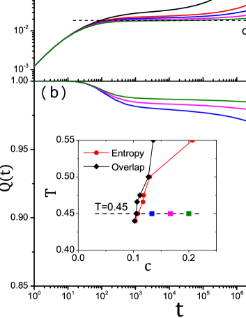
Figure 1: (a) Time dependence of the mean squared displacement $\Delta(t)$ for different concentrations of pinned particles, $c$, at $T=0.45$ for $N=1200$. The horizontal dashed line is the height of the plateau for $c=0.2$. (b) The dynamic overlap function $Q(t)$ at $T=0.45$ for $N=1200$ and concentrations $c$ at which the system is in the equilibrium glass state. The horizontal dashed arrows are the static overlap functions $Q^{\rm(static)}$ evaluated from the parallel tempering simulations. The inset shows the state points for the presented $Q(t)$ in the phase diagram from Ref. Ozawa et al. (2015b).

To probe the relaxation dynamics of the system we focus on $T=0.45$ and increase $c$, thus crossing at around $c=0.1$ the boundary between fluid and glass state (see inset of Fig. 1(b)). Figure 1(a) shows the mean squared displacement (MSD) for different values of $c$: $\Delta(t)=\sum_{i=1}^{(1-c)N}[\langle|{\bf r}_{i}(t)-{\bf r}_{i}(0)|^{2}\rangle]/(1-c)N$. Here $\langle\cdots\rangle$ and $[\cdots]$ are the thermal and disorder averages, respectively. Note that we have averaged the MSD over both species of particles. At intermediate times $\Delta(t)$ has a marked plateau that is related to the usual cage effect observed in glassy systems Binder and Kob (2011) and the horizontal dashed line indicates the plateau height of $\Delta(t)$ at $c=0.2$. Surprisingly we find that even in the equilibrium glass phase, i.e., at this temperature for $c\geq 0.10$ (see SI), $\Delta(t)$ shows at long times a marked increase above this plateau, indicating that the particles can leave their cage. To understand this behavior, we analyze the van-Hove correlation function (see SI) and find that the particles undergo an exchange motions, i.e., the particles tend to be replaced by the same kind of particles (see SI). This seems to explain the upturn of the mean squared displacement. More surprising is the results regarding the collective overlap $Q(t)=\sum_{i,j}[\langle\theta(a-|{\bf r}_{i}(t)-{\bf r}_{j}(0)|)\rangle]$, where $\theta(x)$ is the Heaviside function and $a=0.3$. This function probes the collective relaxation of the system and it is not affected by the particle exchange motions. Figure 1(b) shows that $Q(t)$ decays slightly after the plateau at intermediate times, before it decays to its long time limit (horizontal dashed lines $Q(t\to\infty)=Q^{\rm(static)}$), a quantity that can be calculated with high accuracy directly from the PT simulations. The very high value of $Q^{\rm(static)}>0.85$ and the strong $c-$dependence of this quantity, see Ref. Ozawa et al. (2015b), demonstrates that the explored state points are indeed glass states and hence we can conclude that the system shows subtle and non-trivial relaxation dynamics even in the ideal glass. In the SI we show that this is not an out-of-equilibrium effect.

The presence of this relaxation dynamics is at odds with the results of Ref. Ozawa et al. (2015b) that in the glass phase the configurational entropy $s_{\rm conf}$ seems to be zero (see red circles in Fig. 3(b)), since $s_{\rm conf}=0$ implies that there are no states into which the system can move to relax. In that work $s_{\rm conf}$ was estimated from $s_{\rm tot}-s_{\rm harm}$, where $s_{\rm harm}$ is the entropy of the strictly harmonic solid, i.e., a quantity that can be obtained directly from the vibrational density of states. Our present results rise thus the question whether $s_{\rm conf}$ can indeed be approximated reliably by this difference sciortino1999inherent ; berthier2014novel ; johari2002entropy .

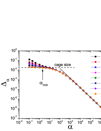
Figure 2: The mean-squared displacement $\Delta_{\alpha}$ at $T=0.45$ for $N=1200$ used for the Frenkel-Ladd thermodynamic integration. The horizontal dashed line is the plateau height for $c=0.2$ shown in Fig. 1(a). The solid line corresponds to the behavior of the Einstein solid, $\Delta_{\alpha}=3/(2\alpha)$.

To advance on this point, we have accurately determined $s_{\rm vib}$ by taking into account the effect of anharmonic vibrations, using two independent approaches. The first one makes use of the idea of Frenkel and Ladd frenkel1984new ; coluzzi1999thermodynamics ; sastry2000evaluation ; Berthier et al. (2017); williams2018experimental of introducing a series of systems which parametrically interpolates between the original system and an Einstein solid, and then to carry out a thermodynamic integration to calculate the vibrational entropy of the original system. In practice we have introduced the Hamiltonian $\beta H(\alpha)=\beta H(0)+\alpha\sum_{i=1}^{(1-c)N}|{\bf r}_{i}-{\bf r}_{0i}|^{2}$, where $H(0)$ is the original Hamiltonian, $\beta=1/T$, $\alpha$ is a spring constant, and ${\bf r}_{0i}$ is the equilibrium configuration of the particle $i$ in the original system. We then measure the MSD $\Delta_{\alpha}=\sum_{i=1}^{(1-c)N}[\langle|{\bf r}_{i}-{\bf r}_{0i}|^{2}\rangle]/(1-c)N$ from which we obtain the entropy

$$s_{\rm FL}=s_{\rm E}(\alpha_{\rm max})+\int_{0}^{\alpha_{\rm max}}\mathrm{d}\alpha\Delta_{\alpha},$$ (1)

where $s_{\rm E}(\alpha_{\rm max})$ is the entropy of the Einstein solid. Figure 2 shows $\Delta_{\alpha}$ for $10^{-1}\leq\alpha\leq 10^{7}$. For $\alpha>10^{4}$, this function follows very closely $3/(2\alpha)$, the behavior of the Einstein solid, and hence we can replace $\Delta_{\alpha}$ by this expression if $\alpha$ is large. The entropy for this Einstein solid is then given by $s_{\rm E}(\alpha_{\rm max})=\frac{3}{2}-3\ln\Lambda-\frac{3}{2}\ln\left(\frac{\alpha_{\rm max}}{\pi}\right)$, where $\Lambda$ is the de Broglie thermal wavelength. In practice we have set $\alpha_{\rm max}=10^{7}$.

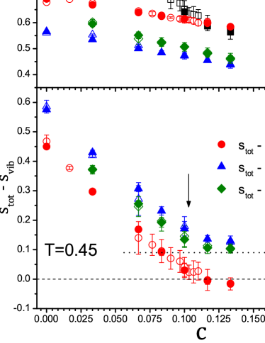
Figure 3: (a) $c-$dependence of the total entropy $s_{\rm tot}$, as well as different estimates of the vibrational entropy. (b) $c-$dependence of $s_{\rm tot}-s_{\rm vib}$. The open and filled symbols are for $N=300$ and $N=1200$, respectively. The horizontal arrows locate $T_{\rm K}(c)$ where the skewness of the overlap distribution becomes zero Ozawa et al. (2015b).

At small $\alpha$, the dependence of $\Delta_{\alpha}$ on $\alpha$ becomes weak suggesting that in this parameter range the particles are vibrating in a cage created by the original Hamiltonian and not by the one of the Einstein solid. However, at the smallest $\alpha$, $\Delta_{\alpha}$ is not completely flat, since at long times the particles are able to escape slowly from their cages. The height of the plateau in $\Delta_{\alpha}$ allows to estimate the amplitude of the vibrations in the real system, i.e., to determine the harmonic and anharmonic component of the motion. Indeed, the height of the plateau in $\Delta_{\alpha}$ is consistent with that of $\Delta(t)$ from Fig. 1(a). To estimate the entropy that is due to the vibrational motion we can evaluate the integral given by Eq. (1) by replacing the contribution to the integral for $\alpha<\alpha_{\rm min}=2$ by $\alpha_{\rm min}\Delta_{\alpha_{\rm min}}$, thus removing in this manner the contribution of the relaxational part to the entropy. The so obtained vibrational entropy $s_{\rm FL}$ is shown in Fig. 3(a) (green diamonds). As expected, the $c-$dependence of $s_{\rm FL}$ is smooth and shows no apparent singularity.

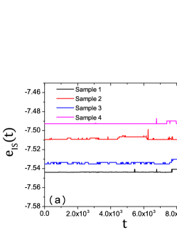
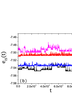
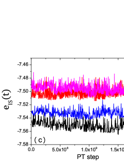
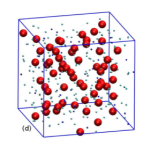
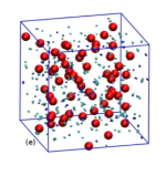
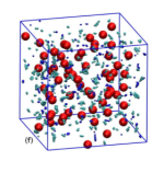
Figure 4: (a-c): $e_{\rm IS}(t)$ at $T=0.45$ and $c=0.2$ for $N=300$ samples with (a) $10^{4}$ and (b) $10^{8}$ MC time step, and (c) $2\times 10^{9}$ PT time step. Different lines correspond to different samples. (d-f): Superposition of the corresponding snapshots (sample 1) of the IS configurations with (d) $10^{4}$ and (e) $10^{8}$ MC time step, and (f) $2\times 10^{9}$ PT time step. Pinned particles are shown in red, and mobile A and B particles are shown in blue and gray, respectively.

The second approach to estimate the anharmonic contribution to the vibrational entropy is to determine the difference between the potential energy of the system and its inherent structure energy and then to subtract the harmonic part, giving thus the anharmonic part of the vibrational energy Mossa et al. (2002); Sciortino (2005). One finds that the so obtained energy is negative which makes that the resulting value for the vibrational entropy, $s_{\rm harm}+s_{\rm anh}$, is smaller than $s_{\rm harm}$ (see blue triangles in Fig. 3(a)), a result that agrees with previous studies Mossa et al. (2002); Sciortino (2005). We see that this quantity agrees very well with our estimate for the vibrational entropy as obtained from the Frenkel-Ladd procedure, indicating that we have determined it with good precision.

Figure 3(b) shows the $c-$dependence of $\Delta s=s_{\rm tot}-s_{\rm vib}$. We see that the improved estimate for $s_{\rm vib}$ makes that now $\Delta s$ no longer goes to zero even at large $c$. Instead it shows a kink at the concentration at which the order parameter had a jump Ozawa et al. (2015b), indicating that at this point the thermodynamic properties of the system have a singular behavior, i.e., that the phase diagram determined in Ref. Ozawa et al. (2015b) is not altered by this improved estimate of $s_{\rm vib}$. Note that we show data for the two system sizes and within the accuracy of the data we see no finite size effects.

To determine the origin of the finite value of $\Delta s$ in the ideal glass phase we probe the potential energy landscape of the system goldstein1969viscous ; stillinger1982hidden ; wales2003energy ; Sciortino (2005); heuer2008exploring . Since at low $T$ the configuration space can be decomposed into the basins of attraction of the inherent structures and vibrations around the IS, an investigation of the PEL should help to understand the nature of the motion of the system. Figure 4(a) shows the time dependence of the IS energy $e_{\rm IS}(t)$, schroder2000crossover ; denny2003trap , for $10^{4}$ steps of MC dynamics at $c=0.2$, a timescale that corresponds to the vibrations inside the cage (see Fig. 1(a)). We see that $e_{\rm IS}(t)$ remains basically constant but shows some spikes indicating that the system accesses for a short period an excited state before it falls back to the original IS, implying that on this time scale only a single IS is relevant heuer2008exploring . Figure 4(d) shows the superposition of the configurations for these IS’s and we see that basically all of them are identical, in agreement with the result from Fig. 1(a) that on this time scale the correlation function does not decay. (For the sake of comparison we show in the SI a corresponding plot for the fluid state.) If the time window is increased by a factor of $10^{4}$, Fig. 4(b), we find that $e_{\rm IS}(t)$ starts to make larger excursions and that these are no longer reversible, indicating that the system explores new IS. This is the reason why on this time scale the correlation function decay slightly, see Fig. 1(b). Figure 4(e) shows that now there are indeed many different IS’s, but since the corresponding positions of the particles form small clusters we can conclude that the configurations are quite similar. Finally we show in Fig. 4(c) the evolution of $e_{\rm IS}(t)$ as obtained from a PT run. We see that in this case the value of $e_{\rm IS}(t)$ fluctuates quite significantly, but that these fluctuations are still smaller than the sample to sample fluctuations and therefore we can infer that there are indeed many different IS’s even in the equilibrium glass state. This conclusion is corroborated by the real space image of the configurations, Fig. 4(f), which now shows quite a few small clusters, i.e., the positions of the particles in the different IS’s differ by a small amount. The presence of these different IS’s is thus the reason for the finite value of $\Delta s$. We emphasize that the clusters seen in Fig. 4(f) do not depend on the length of the PT run.

Our results show that the dynamic and thermodynamic properties of a system with pinned particles give a coherent picture of the equilibrium glass state. Although quantities like the self intermediate scattering function chakrabarty2015dynamics ; chakrabarty2016understanding ; Ozawa et al. (2015a) or the self van Hove function (see SI) do decay to zero, the collective functions do not, once the critical pinning concentration is surpassed. At this transition point the order parameter shows a jump Ozawa et al. (2015b) and the entropy a kink. Our finding that even in the equilibrium glass state particles are able to explore more than one IS indicates that care has to be taken in the definition of the configurational entropy: $s_{\rm conf}$ should not be identified as the difference between the total entropy and the purely vibrational part, since such a definition gives rise to a non-zero $s_{\rm conf}$ even in the ideal glass state. Instead $s_{\rm conf}$ is related to the number of local free energy minima biroli2000inherent and for the case of the pinned system such a minimum is a collection of IS that are geometrically close together. The motion of the particles inside this local free energy minimum is the reason for the partial relaxation of the collective correlation functions. Although the present study concerns a pinned system, it can be expected that bulk systems have a similar behavior since local inhomogeneities in the structure will make that certain regions in the very deeply supercooled liquid are already frozen in, thus leading to a very high value of the viscosity, whereas other regions are still mobile. So the evoked problem with the correct definition of the configurational entropy is likely to exist also in the case of bulk systems.

Supplemental Information

Appendix A Dynamics

A.1 Absence of aging

In Fig. 1(a) of the main text we show that the mean squared displacement (MSD) $\Delta(t)$ of a tagged particle shows at intermediate times the usual plateau found in glassy systems Binder and Kob (2011) but that, surprisingly, the MSD turns at long times upward even when the system is in the ideal glass phase. In order to demonstrate that this upturn is not related to any kind of non-equilibrium dynamics, see e.g. Ref Kob and Barrat (1997), we show in Fig. 5(a) the MSD as obtained for different origins of time. In practice we have taken the trajectory as obtained from the parallel tempering (PT) run and selected five different configurations from that trajectory. For each one of these configurations we have started a standard MC run and have obtained in this manner five different MSDs. The figure shows that these curves are identical with high precision, i.e., they do not depend on the starting configurations. This is hence strong evidence that the upturn of $\Delta(t)$ seen at large times is not related to aging dynamics since in that case one finds that the time for the upturn shifts to increasingly longer times if the age of the system, i.e., the time at which the initial configuration for the MC run was selected, is increased Kob and Barrat (1997). The same conclusion is reached if one considers the time dependence of the overlap, again calculated starting from different starting configurations, see Fig 5(b).

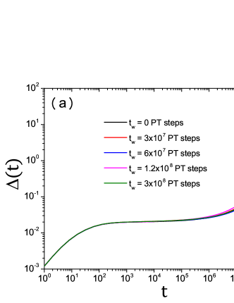
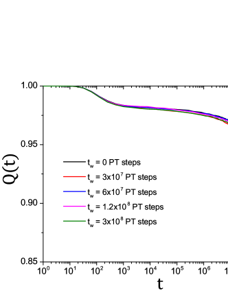
Figure 5: (a): Time dependence of the mean squared displacement $\Delta(t)$ of a single sample at $T=0.45$ and $c=0.167$ for $N=1200$. The starting configurations correspond to different times $t_{\rm w}$ in the PT trajectory and are given in the legend. (b) Same as in panel (a) but now for the collective overlap function $Q(t)$ defined in the main text.

A.2 Dynamics as characterized by the van Hove function

In Fig. 1 of the main text we show the time-dependence of the self dynamics (i.e., the mean squared displacement) as well as a collective correlation function, i.e., the collective overlap function $Q(t)$. In Ref. Ozawa et al. (2015a) we have argued that because of the presence of the pinned particles the self correlation functions behave very differently from the collective ones in that the latter will decay to a plateau with finite value whereas the former will go to zero as in a normal liquid. To understand better the motion of the particles in real space it is useful to look at the self and distinct parts of the van Hove correlation functions Hansen and McDonald (2006).

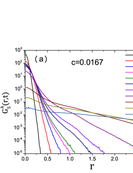
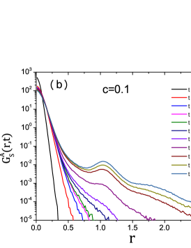
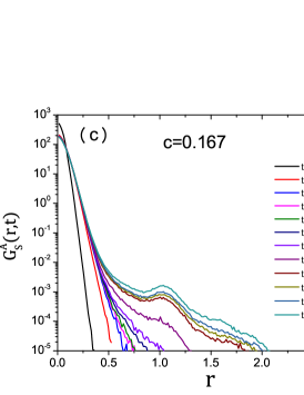
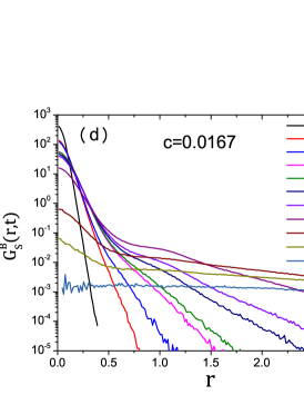
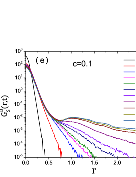
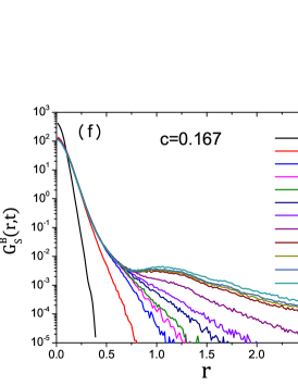
Figure 6: Self part of the van Hove correlation function at $T=0.45$ and different values of $c$ for $N=1200$. (a)-(c): Species A, (d)-(f): Species B.

The self part of the van Hove function is defined by

$$G_{\rm s}^{\alpha}(r,t)=\frac{1}{(1-c)N_{\alpha}}\sum_{i=1}^{(1-c)N_{\alpha}}\left[\left\langle\delta(r-|{\bf r}_{i}(0)-{\bf r}_{i}(t)|)\right\rangle\right],$$ (2)

where $N_{\alpha}$ is the number of particles of species $\alpha$. Here $\alpha,\beta\in\{{\rm A},{\rm B}\}$. The distinct part of the van Hove function is defined by

$$G_{\rm d}^{\alpha\alpha}(r,t) = \frac{N}{(1-c)N_{\alpha}^{2}}\sum_{i=1}^{(1-c)N_{\alpha}}\sum_{j(\neq i)}^{(1-c)N_{\beta}}\left[\left\langle\delta(r-|{\bf r}_{i}(0)-{\bf r}_{j}(t)|)\right\rangle\right],$$ (3)

$$G_{\rm d}^{\alpha\beta}(r,t) = \frac{N}{(1-c)N_{\alpha}N_{\beta}}\sum_{i=1}^{(1-c)N_{\alpha}}\sum_{j}^{(1-c)N_{\beta}}\left[\left\langle\delta(r-|{\bf r}_{i}(0)-{\bf r}_{j}(t)|)\right\rangle\right]\quad(\alpha\neq\beta).$$ (4)

The $r$-dependence of $G_{\rm s}(r,t)$ is shown in Fig. 6 for temperature $T=0.45$ and different pinning concentrations $c$. For $c=0.0167$, i.e., when the system is very similar to a glassy bulk system, the $G_{\rm s}(r,t)$ shows at very short times the Gaussian behavior expected for a harmonic system since on this time scale the particle explores its local cage. With increasing time the particle leaves that cage and accesses larger distances before becoming diffusive. If the concentration is increased to $c=0.1$, Fig. 6(b), we see that at large times the distribution function has a marked peak at $r\approx 1$, i.e., the particle hops by a nearest neighbor distance. Small peaks are seen at larger distances at $r\approx 2$ and 2.7, which correspond to the second and third nearest neighbor distances Li et al. (2015). If $c$ is increased even more, Fig. 6(c), the form of $G_{\rm s}(r,t)$ is not altered appreciably, although the probability at large distances decreases by more than one order of magnitude. Thus we can conclude that the presence of the pinned particles change the nature of the motion from a flow-like motion at low $c$ to a hopping motion at intermediate and high $c$.

The self part of the van Hove functions discussed so far were for the A particles which are larger and thus less mobile than the B particles. In Figs. 6 (d)-(f) we show the same quantity for the B particles. In agreement with the results for the bulk system Kob and Andersen (1995), we see that already for very low concentration there is a small peak at $r\approx 1$, i.e., the particles show some tendency for a hopping dynamics. If $c$ is increased the peak becomes more pronounced but remains smaller than the corresponding peak for the A particles.

The $r$-dependence of the distinct part of the van Hove function is shown in Fig. 7. By definition, $G_{\rm d}^{\alpha\beta}(r,t=0)$ is the radial distribution function, which is zero at $r\lesssim 1$ and with several distinct peaks corresponding to the nearest or next nearest distances. All panels show that the hole of $G_{\rm d}^{\alpha\beta}(r,t=0)$ at $r\lesssim 1$ is filled up by other particles at longer times. For the A-A component, panels (a)–(c), one observes that, for a fixed $t$, the peak developing at $r=0$ becomes sharper and the height of the peak becomes lower as the $c$ is increased. We find a very similar behavior for the B-B component, panels (d)–(f). The peaks are slightly higher than those of the A–A component because the B particles can undergo a hopping motion more easily since they are smaller than the A particle. On the contrary, for the A-B component, panels (g)–(i), the growth of the peak is somewhat weaker. These results imply that, in the hopping motion, the particles tend to be replaced by the same kind of particles.

Note that, although the exchange of two particles of the same type allows that the particles undergo a diffusive motion at large times, the underlying structure does not change (i.e., it is like the diffusion of defects in a crystal). Hence this type of motion will not give rise to a change in the overlap function. This is different for the exchange of an A particle with a B particle since an exchange of unlike particles will lead to a non-equivalent configurations. As mentioned above, we recognize that in this case the peak at the origin is now much smaller which is explained by the fact that the size of the A particle is significantly larger than the one of the B particles and hence it is difficult to swap the position of the unlike particles. Nevertheless, at sufficiently long times a small peak can be observed even in this case and hence the system is indeed able to access new configurations, in agreement with the findings on the entropy and PEL analysis presented in the main text.

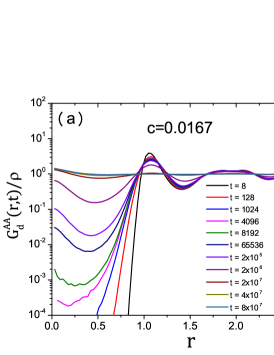
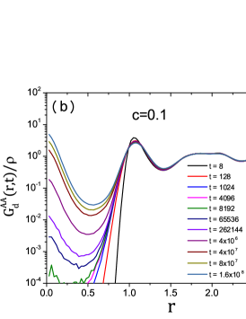
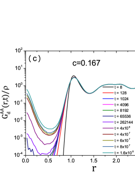
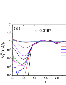
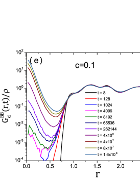
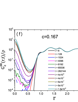
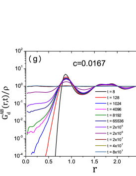
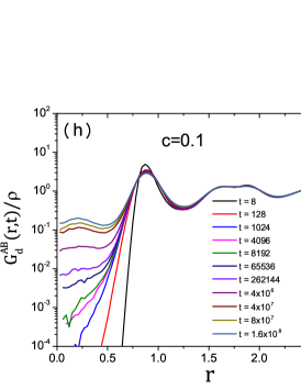
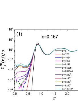
Figure 7: Distinct part of the van Hove correlation function at $T=0.45$ and different values of $c$ for $N=1200$. (a)-(c): A-A correlation, (d)-(f): B-B correlation, (g)-(i): A-B correlation.

Appendix B Thermodynamics

B.1 Anharmonic contribution for the vibrational entropy

In this section we show how to evaluate the anharmonic contribution for $s_{\rm vib}$. Details of this method are described in Refs. Mossa et al. (2002); Sciortino (2005) for the bulk system. The extension of the method to the pinned system is straightforward.

The anharmonic contribution of the total potential energy $U_{\rm anh}(c,T)$ is given by

$$U_{\rm anh}(c,T)=U(T)-U_{\rm IS}(c,T)-\frac{3}{2}(1-c)NT,$$ (5)

where $U(T)$ and $U_{\rm IS}(c,T)$ are, respectively, the equilibrium bulk potential energy and the inherent structure energy of the pinned system. The last term in Eq. (5) is the energy of the harmonic vibrations of $(1-c)N$ mobile particles.

Making a $T-$expansion of $U_{\rm anh}(c,T)$ around $T=0$ gives

$$U_{\rm anh}(c,T)=\sum_{k=2}C_{k}(c)T^{k},$$ (6)

where $C_{k}(c)$ are $T-$independent coefficients. Note that the sum starts at $k=2$ since the system is completely harmonic in the low temperature limit.

The anharmonic contribution for the vibrational entropy $S_{\rm anh}(c,T)$ is given by

$$S_{\rm anh}(c,T)=\int_{0}^{T}dT^{\prime}\frac{1}{T^{\prime}}\frac{\partial U_{\rm anh}(c,T^{\prime})}{\partial T^{\prime}}.$$ (7)

Note that we set $S_{\rm anh}(c,T=0)=0$.

Substituting Eq. (6) to Eq. (7), we obtain

$$S_{\rm anh}(c,T)=\sum_{k=2}\frac{k}{k-1}C_{k}(c)T^{k-1}.$$ (8)

To evaluate $S_{\rm anh}$ we have used the following numerical procedure: First we use the simulations to obtain $U_{\rm anh}(c,T)$ and then the coefficients $C_{k}(c)$’s are obtained by fitting $U_{\rm anh}(c,T)$ to a polynomial function of $T$. In practice we use the first two terms, $C_{2}(c)$ and $C_{3}(c)$, for this fitting Mossa et al. (2002). Finally $S_{\rm anh}(c,T)$ is evaluated using Eq. (8). It is clear that the signs of $C_{k}(c)$’s determine the sign of $S_{\rm anh}(c,T)$. In Fig. 8(a), the simulation data of $U_{\rm anh}(c,T)$ are plotted for several values of $c$. The solid lines are fits down to $T=0$. The resulting $s_{\rm anh}(c,T)=S_{\rm anh}(c,T)/(1-c)N$ are shown in Fig. 8(b). We find that $s_{\rm anh}(c,T)$ is small and negative for all $c$’s and $T$’s considered, in agreement with the results from Refs. Mossa et al. (2002); Sciortino (2005).

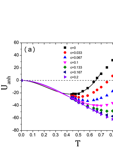
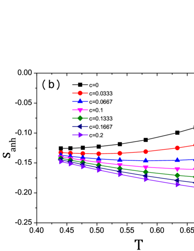
Figure 8: (a) Temperature dependence of the anharmonic potential energy $U_{\rm anh}(c,T)$ for several values of $c$’s. (b) Temperature dependence of the anharmonic contribution of the vibrational entropy $s_{\rm anh}(c,T)=S_{\rm anh}(c,T)/(1-c)N$ per a particle for several values of $c$. The data in (a) (b) are from $N=1200$.

B.2 Overlap and Finite Size Effects

In Fig. 9(a) we show the distribution $P(Q)$ of the overlap $Q_{\alpha\beta}$ between two configurations $\alpha$ and $\beta$ which is defined by

$$Q_{\alpha\beta}=\frac{1}{N}\sum_{i,j}^{N}\theta(a-|\mathbf{r}_{i}^{\alpha}-\mathbf{r}_{j}^{\beta}|),$$ (9)

where $\theta(x)$ is the Heaviside function, $\mathbf{r}_{i}^{\alpha}$ is the position of the $i$-th particle in the configuration $\alpha$, and the length-scale $a$ is set to $0.3$ Kob and Berthier (2013). For small $c$ we see a single peak at small $Q$ which shows that for weak pinning the overlap between two typical equilibrium configurations is small. For intermediate $c$ we find a pronounced double peak structure indicating the coexistence of states that have a low overlap and states that have a high overlap with each other. If $c$ is increased further one finds only a single peak at large $Q$, i.e., most configurations are very similar. These results are for $N=1200$ particles and are qualitatively very similar to the one for $N=300$ presented in Ref. Ozawa et al. (2015b). To show the $N-$independence more quantitatively, we present in Fig. 9(b) the $c-$dependence of the mean overlap $Q^{\rm(static)}$ which is given by the first moment of $P(Q)$. We see that within the accuracy of the data the curves for $N=300$ coincide with the one for $N=1200$. We also observe that the $N$-dependence of $s_{\rm tot}-s_{\rm vib}$ at the lowest temperature is small (see Fig. 9(c)). This result is somewhat surprising since one expects noticeable finite size effect in the vicinity of the ideal glass transition due to some growing static correlation lengths Fullerton and Jack (2014); Takahashi and Hukushima (2015) and, thus of the $N$-dependence of the order-parameter $Q^{\rm(static)}$. One possibility to rationalize the absence of such finite size effects is that the finite size exponents is very small in the temperature range which we explore Cammarota and Biroli (2013). In order to verify this, one must study lower temperatures with more efficient algorithms or consider other model systems Ninarello et al. (2017); Berthier et al. (2017).

On this point, we note that our results are not very sensitive to the temperature, see e.g. Fig. 9(c) for the difference $s_{\rm tot}-s_{\rm vib}$, and therefore we expect them to be relevant also at lower temperatures.

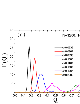
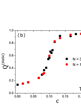
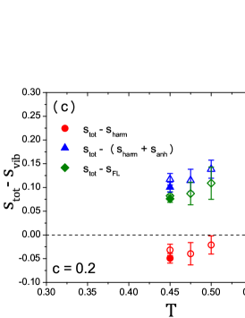
Figure 9: (a) Distribution function $P(Q)$ of the overlap for different concentration of pinned particles. $T=0.45$ and $N=1200$. (b) $c-$dependence of the average overlap for $N=300$ and $N=1200$ at $T=0.45$. (c) $T-$dependence of the configurational entropy along $c=0.2$. The open and filled symbols are for $N=300$ and $N=1200$, respectively.

Appendix C Potential energy landscape

C.1 Snapshot

In Fig. 4 of the main text we show the superposition of snapshots of IS configurations for $N=300$ particles. In Fig. 10 we present similar data for $N=1200$. Panel (a) shows the snapshots for $c=0.0167$, i.e., the case where the system is still in the liquid-like regime. We see that the position of the particles basically fill out all the accessible space, with the exception of the region around the pinned particles. For $c=0.08$, i.e., slightly below the transition, some empty regions can be spotted, indicating that now the particles can no longer access the whole space, panel (b). If the concentration is increased to $c=0.167$, i.e., a state that is deep in the glass state, most of the IS are very similar and hence the available configuration space has become very small, panel (c). However, even in this case we find that there are small clusters of particle positions that indicate that a glass state is composed of many different IS, which is thus the reason for having a non-trivial entropy.

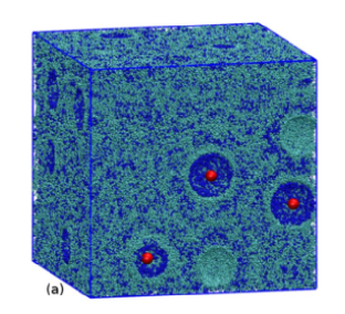
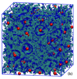
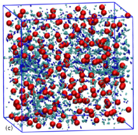
Figure 10: Snapshot of IS for $N=1200$, $T=0.45$. The size of the box is 10.0, pinned particles are shown in red, and mobile A and B particles are shown in blue and gray, respectively. (a) $c=0.0167$ (fluid), (b) $c=0.08$ (fluid close to the ideal glass transition), and (c) $c=0.1667$ (glass).

References

- Binder and Kob (2011) K. Binder and W. Kob, Glassy Materials and Disordered Solids: An Introduction to their Statistical Mechanics (World Scientific, 2011).
- Kob and Barrat (1997) W. Kob and J.-L. Barrat, Phys. Rev. Lett. 78, 4581 (1997).
- Ozawa et al. (2015a) M. Ozawa, W. Kob, A. Ikeda, and K. Miyazaki, Proc. Natl. Acad. Sci. USA 112, E4821 (2015a).
- Hansen and McDonald (2006) J.-P. Hansen and I. McDonald, Theory of Simple Liquids (Academic Press, 2006).
- Li et al. (2015) Y.-W. Li, Y.-L. Zhu, and Z.-Y. Sun, J. Chem. Phys. 142, 124507 (2015).
- Kob and Andersen (1995) W. Kob and H. C. Andersen, Phys. Rev. E 51, 4626 (1995).
- Mossa et al. (2002) S. Mossa, E. La Nave, H. Stanley, C. Donati, F. Sciortino, and P. Tartaglia, Phys. Rev. E 65, 041205 (2002).
- Sciortino (2005) F. Sciortino, J. Stat. Mech. Theory Exp. 2005, P05015 (2005).
- Kob and Berthier (2013) W. Kob and L. Berthier, Phys. Rev. Lett. 110, 245702 (2013).
- Ozawa et al. (2015b) M. Ozawa, W. Kob, A. Ikeda, and K. Miyazaki, Proc. Natl. Acad. Sci. USA 112, 6914 (2015b).
- Fullerton and Jack (2014) C. J. Fullerton and R. L. Jack, Phys. Rev. Lett. 112, 255701 (2014).
- Takahashi and Hukushima (2015) T. Takahashi and K. Hukushima, Phys. Rev. E 91, 020102 (2015).
- Cammarota and Biroli (2013) C. Cammarota and G. Biroli, J. Chem. Phys. 138, 12A547 (2013).
- Ninarello et al. (2017) A. Ninarello, L. Berthier, and D. Coslovich, Phys. Rev. X 7, 021039 (2017).
- Berthier et al. (2017) L. Berthier, P. Charbonneau, D. Coslovich, A. Ninarello, M. Ozawa, and S. Yaida, Proc. Natl. Acad. Sci. USA , 201706860 (2017).