EM short = EM, long = electromagnetic, GW short = GW, long = gravitational wave, CFI short = CFI, long = classical Fisher information, CRB short = CRB, long = Cramér-Rao bound, QCRB short = QCRB, long = quantum Cramér-Rao bound, QFI short = QFI, long = quantum Fisher information, POVM short = POVM, long = positive operator valued measurement, SNL short = SNL, long = shot-noise limit, SQL short = SQL, long = standard quantum limit,

Fundamental Quantum Limits of Multicarrier Optomechanical Sensors

Abstract

Optomechanical sensors involving multiple optical carriers can experience mechanically mediated interactions causing multi-mode correlations across the optical fields. One instance is laser-interferometric gravitational wave detectors which introduce multiple carrier frequencies for classical sensing and control purposes. An outstanding question is whether such multi-carrier optomechanical sensors outperform their single-carrier counterpart in terms of quantum-limited sensitivity. We show that the best precision is achieved by a single-carrier instance of the sensor. For the current LIGO detection system this precision is already reachable.

Introduction.—The use of quantum-mechanical systems and non-classical properties for high-precision estimation tasks has attracted interest in a number of sensing schemes, including in laser-interferometric GW detectors Caves (1981); Kimble et al. (2001); The LIGO Scientific Collaboration (2011); Demkowicz-Dobrzański et al. (2013); Miao et al. (2017) and related problems Tsang et al. (2011); Lang and Caves (2013), magnetometry Sheng et al. (2013); Baumgratz and Datta (2016), and atomic clocks Bollinger et al. (1996); Macieszczak et al. (2014). Direct detection of GW was one of the earliest problems to demand such analysis Braginsky and Khalili (1996), suggesting use of non-classical light—squeezed vacuum states—to improve precision Caves (1981); Schnabel (2017).

Sensing mechanical displacements optically, such as in laser-interferometric GW detectors Braginsky and Khalili (1992); Danilishin and Khalili (2012), relies on interactions between optical and mechanical degrees of freedom is the domain of optomechanical Chen (2013); Aspelmeyer et al. (2014) sensors. Light incident on a mechanical oscillator causes the mechanical oscillator to act as an active element which produces squeezing of optical modes Braginsky and Manukin (1967); Kimble et al. (2001)—the so-called ponderomotive squeezing. Such squeezing acts as a noise source constraining the current generation of laser-interferometric GW detectors Braginsky and Khalili (1992); Kimble et al. (2001) due to anti-squeezing of the quadrature in which the signal is encoded which manifests as a measurement backaction, with techniques to avoid such backaction drawing significant interest Tsang and Caves (2010); Ockeloen-Korppi et al. (2016); Møller et al. (2017). The same effect has been demonstrated as a squeezed light source Brooks et al. (2012); Safavi-Naeini et al. (2013); Purdy et al. (2013a), which can potentially improve sensors’ precision Caves (1981); Kimble et al. (2001); Schnabel (2017).

The extension to multi-mode optomechanical systems has proven fruitful in both the many mechanical Nielsen et al. (2017) and optical Lee et al. (2015); Slatyer et al. (2016) mode scenarios, as well as for optical frequency conversion Hill et al. (2012); Andrews et al. (2014). This includes sensors such as laser-interferometric GW detectors, particularly those encompassing modifications which utilise multiple laser frequencies: so-called multi-carrier interferometers. Originally implemented in Advanced LIGO for classical sensing and control purposes Izumi et al. (2012); Staley et al. (2014), a second carrier can improve the low-frequency sensitivity by partially cancelling the strong backaction of the main carrier Rehbein et al. (2007); Miao et al. (2014). Multiple carriers can provide a means to enhance the sensitivity and surpass the SQL Braginsky and Khalili (1992) by using the optical spring effect, while not suffering from the instabilities associated with the single-carrier case and allowing for some shaping of the sensitivity curves Rehbein et al. (2008); Korobko et al. (2015). The value of multiple carriers in improving the sensors’ fundamental quantum limit, which is more stringent than the SQL, remains open.

In this Letter we provide the fundamental quantum limits on the precision of multi-carrier optomechanical sensors, including laser-interferometric GW detectors, using quantum metrology techniques. These limits are imposed by the classical and quantum Fisher information—via the CRB on precision of an estimator—from quantum estimation theory Holevo (2011); Braunstein and Caves (1994); Hayashi (2005); Paris (2009); Tóth and Apellaniz (2014); Demkowicz-Dobrzański et al. (2015). Our multimode analysis includes optical loss at the output and squeezed light injection; as well as the optomechanical interaction—the ponderomotive squeezing effect.

Multi-mode quantum states have been studied in quantum metrology Pinel et al. (2012); Humphreys et al. (2013); Friis et al. (2015); Ciampini et al. (2016); Gagatsos et al. (2016). By including a noise source which itself introduces multi-mode correlations, ponderomotive squeezing, for the first time we show that for a large class of optomechanical sensors multiple carriers are no better than single carriers. Hitherto neglected in estimation-theoretic quantum metrology studies of GW detectors Lang and Caves (2013); Demkowicz-Dobrzański et al. (2013) ponderomotive squeezing dominates the low-frequency quantum noise of GW detectors Kimble et al. (2001) as well as smaller optomechanical systems Purdy et al. (2013b); Teufel et al. (2016); Cripe et al. (2018). We bridge this gap, providing analytical expressions for the fundamental quantum limits of multi-mode optomechanical sensors featuring ponderomotive squeezing. This should guide the development of novel optomechanical sensors and the improvement of existing ones. Our large complement of results can be navigated using Table 1.

Input & output	Fundamental limit	Freq. dependent homodyne	Signal quadrature homodyne
Squeezed & lossy	Eq. (12)	Eq. (13)	Eq. (14)
Identically squeezed & lossy	Eq. (16)	Eq. (16)	Eq. (18)
Unsqueezed & lossy	Eq. (20)	Eq. (20)	Eq. (21)
Squeezed & lossless	Eq. (22)	Eq. (22)	Supplementary material Note (1)

Table 1: Expressions for precision of various interferometer limits. The unsqueezed and lossless case can be most readily recognised from the lossy and unsqueezed case with limit $\eta=1$. We provide some discussion of these results in the context of LIGO detector in Sec. VIII of the Supplementary material Note (1).

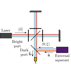
Figure 1: An instance of an optomechanical sensor—a laser-interferometric gravitational wave detector with multiple different frequency carrier-modes. Circulating light couples to the mechanical motion of the mirrors inside the interferometer arms. $\mathbf{\hat{a}}$ and $\mathbf{\hat{b}}$ describe the field of the carrier-mode sidebands, entering and exiting the interferometer respectively at the dark port.

Framework.—We describe the optical part of our optomechanical sensor with a linear input-output relation

$$\mathbf{\hat{b}}(\Omega)=\mathcal{M}(\Omega)\mathbf{\hat{a}}(\Omega)+h(\Omega)\vec{\mathcal{V}}(\Omega),$$ (1)

where $\mathcal{M}(\Omega)$ is a complex matrix which determines a Bogoliubov transformation between the incoming and outgoing fields, and $h(\Omega)\vec{\mathcal{V}}(\Omega)$ is a displacement vector which encodes the parameter $h(\Omega)$. Such input-output relations are typically expressed in terms of the two-photon formalism Caves and Schumaker (1985); Schumaker and Caves (1985), using the two operators $\hat{a}_{1}^{(\omega)}=(\hat{a}_{\omega+\Omega}+\hat{a}_{\omega-\Omega}^{\dagger})/\sqrt{2},$ and $\hat{a}_{2}^{(\omega)}=-i(\hat{a}_{\omega+\Omega}-\hat{a}_{\omega-\Omega}^{\dagger})/\sqrt{2}.$ We introduce $d$ pairs of such operators $\{\hat{a}_{1}^{(\omega_{1})},\hat{a}_{2}^{(\omega_{1})},\cdots,\hat{a}_{2}^{(\omega_{d})}\}$ to describe the EM fields in an interferometer driven by light of multiple carrier frequencies $\{\omega_{1},\omega_{2},\cdots,\omega_{d}\}$. From these creation/annihilation operators, we can form hermitian position ($\hat{x}_{1,2}^{(\omega)}$) and momentum ($\hat{p}_{1,2}^{(\omega)}$) operators, spanning the same phase space and obeying suitable commutation relations Note (1).

Suppressing the $\Omega$ argument for brevity; we focus on the case where we wish to estimate the size of the displacement $h$, with $\mathcal{M}$ and $\mathcal{V}$ consisting of the $2{\times}2$ and $2{\times}1$ blocks Rehbein et al. (2008); Miao et al. (2014), see also Sec. II of the supplementary material Note (1)

$$\begin{gathered}\mathcal{M}_{jk}=e^{i(\beta_{j}+\beta_{k})}\begin{pmatrix}\delta_{jk}&0\\ -\chi\sqrt{\kappa_{j}\kappa_{k}}&\delta_{jk}\end{pmatrix},\\ \mathcal{V}_{j}=\frac{e^{i\beta_{j}}}{h_{\text{SQL}}}\begin{pmatrix}0\\ \chi\sqrt{2\kappa_{j}}\end{pmatrix},\end{gathered}$$ (2)

where $\delta_{ij}$ is the Kronecker delta, $\beta_{i}$ are phases, $\kappa_{i}\geq 0$. $\chi\in\{-1,1\}$ is the sign of the mechanical response and can be taken to be positive, since one with a negative response is identical to one with a positive $\chi$ with a fixed phase shift preceding and succeeding it, which can be captured by rotating input squeezing and output homodyne angles respectively. The attainable precisions are thus directly related; see Sec. II of the supplementary material Note (1). The presence of the $\sqrt{\kappa_{j}\kappa_{k}}$ term on the off-diagonals produces a multi-mode squeezing across all the optical modes, which is ponderomotive in origin. The ponderomotive squeezing introduced with a single optical mode—with frequency $\omega$—is itself multi-mode with correlations between the $\omega+\Omega$ and $\omega-\Omega$. When multiple optical fields are used they each affect the mechanical motion and in turn the mechanical motion causes squeezing of each optical mode leading to entanglement between $\omega_{j}+\Omega$ and $\omega_{k}+\Omega$ optical modes.

In the case of a multi-carrier laser-interferometric GW detector as in Fig. 1 in the tuned configuration, $\kappa_{i}$ is the normalised intensity of the $i$-th carrier

$$\kappa_{i} =\frac{16I_{i}\omega_{i}\gamma_{i}}{mcL\Omega^{2}\left(\gamma_{i}^{2}+\Omega^{2}\right)}, h_{\text{SQL}} =\sqrt{\frac{8\hbar}{m\Omega^{2}L^{2}}},$$ (3)

where $I_{i}$ is the arm cavity power of the $i$th mode, $\omega_{i}$ the frequency of the $i$th mode, $\gamma_{i}$ the arm cavity half-bandwidth of the $i$th mode, $m$ the test mass, and $L$ the interferometer arm length Danilishin and Khalili (2012). The signal-recycling mirror Buonanno and Chen (2001, 2002, 2003); McClelland et al. (2017) introduces more involved input-output relations but at low-frequencies where radiation-pressure dominates the quantum noise they can be approximated with the same form of Eq. (2) Corbitt et al. (2006). Interferometer modifications such as the quantum speed meter Purdue and Chen (2002); Danilishin and Khalili (2012); McClelland et al. (2017) also have the same form of input-output relations as Eq. (2) and our results can be applied directly with appropriate definition of $\kappa_{i}$.

As Eq. (1) is a linear mapping between creation operators, the optical fields through the sensor evolve under a Gaussian unitary Adesso et al. (2014). Common input states such as (squeezed) vacuum are themselves Gaussian Caves (1981); Kimble et al. (2001); The LIGO Scientific Collaboration (2011), therefore the output state can be taken as Gaussian for relevant cases. From the evolution of the quadrature operators

$$\mathbf{\hat{x}}^{\prime} =\frac{\mathcal{M}\mathbf{\hat{a}}+\mathcal{M}^{*}\mathbf{\hat{a}}^{\dagger}+h\vec{\mathcal{V}}+h^{*}\vec{\mathcal{V}}^{*}}{\sqrt{2}},$$ (4)

$$\mathbf{\hat{p}}^{\prime} =\frac{\mathcal{M}\mathbf{\hat{a}}-\mathcal{M}^{*}\mathbf{\hat{a}}^{\dagger}+h\vec{\mathcal{V}}-h^{*}\vec{\mathcal{V}}^{*}}{i\sqrt{2}},$$

we can extract the displacement and symplectic operators

$$\vec{d}_{\mathcal{V}}=\sqrt{2}\begin{pmatrix}\Re[h\vec{\mathcal{V}}]\\ \Im[h\vec{\mathcal{V}}]\end{pmatrix}, \mathcal{S}_{\mathcal{M}}=\begin{pmatrix}\Re\mathcal{M}&-\Im\mathcal{M}\\ \Im\mathcal{M}&\Re\mathcal{M}\end{pmatrix},$$ (5)

where $\Re$ and $\Im$ denote the real and imaginary parts. The first- and second-order moments $\vec{d}_{\text{In}}$ and $\sigma_{\text{In}}$ of a Gaussian input evolve through the sensor as

$$\vec{d}_{\text{Out}} =\vec{d}_{\text{In}}+\vec{d}_{\mathcal{V}}, \sigma_{\text{Out}} =\mathcal{S}_{\mathcal{M}}\sigma_{\text{In}}\mathcal{S}_{\mathcal{M}}^{T}.$$ (6)

Quantum estimation.—The CRB and QCRB are successive lower bounds on the variance $(\Delta\tilde{h})^{2}=\mathbb{E}[\tilde{h}^{2}]-\mathbb{E}[\tilde{h}]^{2}$ of an unbiased estimator $\tilde{h}$ for a parameter $h$ which parameterises some probability distribution $P(\vec{x}|h)$ and in turn some state $\rho(h)$ which is given by

$$(\Delta\tilde{h})^{2}\geq\frac{1}{F(h)}\geq\frac{1}{H(h)},$$ (7)

where $F(h)$ is the CFI and $H(h)$ the QFI. The CFI depends on the sampled probability distribution as Braunstein and Caves (1994); Hayashi (2005); Paris (2009); Tóth and Apellaniz (2014); Demkowicz-Dobrzański et al. (2015)

$$F(h)=\sum\limits_{\{\vec{x}\}}\frac{1}{P(\vec{x}|h)}\left(\frac{\partial P(\vec{x}|h)}{\partial h}\right)^{2},$$ (8)

and the QFI can be derived from the fidelity as Braunstein and Caves (1994); Hayashi (2005); Paris (2009); Tóth and Apellaniz (2014); Demkowicz-Dobrzański et al. (2015)

$$H(h)=-4\lim_{\text{d}h\to 0}\left\{\frac{\partial^{2}}{\partial(\text{d}h)^{2}}\mathcal{F}(\rho_{h},\rho_{h+\mathrm{d}h})\right\},$$ (9)

where the fidelity is $\mathcal{F}(\rho_{1},\rho_{2})=\mathrm{Tr}\left[\sqrt{\sqrt{\rho_{1}}\rho_{2}\sqrt{\rho_{1}}}\right]$. For single-parameter estimation there always exists some POVM for which the second inequality of Eq. (7) is saturated Braunstein and Caves (1994); Paris (2009).

For a parameter encoded only in the displacements of a Gaussian state the QFI is Pinel et al. (2012); Monras (2013); Gao and Lee (2014); Šafránek et al. (2015)

$$H(h)=2(\partial_{h}\vec{d})^{T}\sigma^{-1}(\partial_{h}\vec{d}),$$ (10)

where $\vec{d}$ and $\sigma$ are the displacement vector and covariance matrix of the Gaussian state respectively.

$\mathcal{M}$ and $\vec{\mathcal{V}}$ can be expressed as $\mathcal{M}=BMB$ and $\vec{\mathcal{V}}=B\vec{V}$, where $B=\operatorname{diag}\left(e^{i\beta_{1}}\mathbb{1}_{2\times 2},\cdots,e^{i\beta_{d}}\mathbb{1}_{2\times 2}\right)$, and $M$ and $\vec{V}$ are real for all cases given by Eq. (2). With an input state that can be written as $\sigma_{\text{In}}=\sigma_{0}\oplus\sigma_{0}$, the QFI for the parameter $|h|$ is then (see Sec. III of the supplementary material Note (1)) given by

$$H(|h|)=4\vec{V}^{T}\left(M\sigma_{0}M^{T}\right)^{-1}\vec{V}.$$ (11)

As Eq. (11) is independent of $\arg(h)$ we henceforth take $h$ to be real and positive.

To compare with the spectral noise density which is typically used to describe the sensitivity of sensors Braginsky and Khalili (1992); Kimble et al. (2001); Miao et al. (2014) the CRB should be multiplied by $4$ as $S_{n}(\Omega)=4/F(h)$, see Sec. IV of the supplementary material Note (1). Our bounds therefore have a pre-factor $h_{\text{SQL}}^{2}/8$ in comparison to results using the single-sided spectral density where the equivalent pre-factor is $h_{\text{SQL}}^{2}/2$ Kimble et al. (2001); Miao et al. (2014).

Sensor scheme.—From Eq. (2) the optical modes are coupled through a multi-mode squeezing, which are weighted through the optical intensities of each mode. We model optical loss at the detector by mixing the outgoing modes $\mathbf{\hat{b}}$ with a (Gaussian) environment at a beam splitter with transmittivity $\eta$ as $\mathbf{\hat{b}}\to\sqrt{\eta}\mathbf{\hat{c}}+\sqrt{1-\eta}\mathbf{\hat{n}},$ with reflected light dumped in a set of modes $\mathbf{\hat{n}}$ which are traced out from the final state leaving only the measurable modes $\mathbf{\hat{c}}$ accessible. The effect on the final state is

$$\vec{d}\to\sqrt{\eta}\vec{d}, \sigma\to\eta\sigma+(1-\eta)\sigma_{\text{Loss}},$$

where we will take the input from the environment to be pure vacumm, namely $\sigma_{\text{Loss}}=\mathbb{1}$.

Externally squeezed light inputs can enhance precision Caves (1981); Kimble et al. (2001); The LIGO Scientific Collaboration (2011) and has already been demonstrated in current GW detectors The LIGO Scientific Collaboration (2011, 2013). With multi-mode interferometers one feasible generalisation is to have parallel squeezing for the sidebands of each carrier frequency, with some squeezing $\xi_{j}=r_{j}e^{i\phi_{j}}$ in the $\hat{x}_{1}^{(j)}$ and $\hat{x}_{2}^{(j)}$ modes.

Our main result is the fundamental quantum limit to the precision of the interferometer scheme described—with arbitrary intensity and external squeezing in each mode—which is

$$\left(\Delta h\right)^{2}\geq\frac{h_{\text{SQL}}^{2}}{8}\left\{\frac{\left[1-(1-\eta)\eta\langle S\Gamma\rangle\right]^{2}}{\eta\left[(1-\eta)\langle\Gamma\rangle+\eta\langle Q\Gamma\rangle\right]}+(1-\eta)\langle P\Gamma\rangle\right\},$$ (12)

where we define the diagonal matrices $Q_{ii}=\left(\cosh 2r_{i}+\sinh 2r_{i}\cos 2\phi_{i}\right)$, $S_{ii}=\sinh 2r_{i}\sin 2\phi_{i}$, $\Gamma_{ii}=\left\{\left[(1-\eta)^{2}+\eta^{2}\right]+2\eta(1-\eta)\cosh 2r_{i}\right\}^{-1}$, $P=\eta\mathbb{1}+(1-\eta)Q$, and $\langle A\rangle$ is defined as $\sum\limits_{i,j=1}^{d}\sqrt{\kappa_{i}\kappa_{j}}A_{ij}$. The dependency on carrier mode intensity is a function of summations over $\kappa_{i}$ weighted by various functions of the squeezing magnitude and angle in the respective mode.

Attainability of quantum-limited precision requires the application of specific measurement schemes on the quantum system. Homodyne detection covers both measurement of the signal quadrature which is in active use Kimble et al. (2001); Hild et al. (2009); Fricke et al. (2012); Danilishin and Khalili (2012) and the more general frequency-dependent homodyne Kimble et al. (2001); Danilishin and Khalili (2012); Miao et al. (2014); McClelland et al. (2017) that measures along a different quadrature for each frequency mode $\Omega$ of the signal. Both of these can be modelled by performing homodyne detection on some quadrature $\sin\theta_{i}\hat{x}^{(i)}_{1}+\cos\theta_{i}\hat{x}^{(i)}_{2}$ for each carrier mode, in which $\theta_{i}$ can be frequency dependent. This provides a precision of

$$\left(\Delta h\right)^{2}\geq\frac{h_{\text{SQL}}^{2}}{8}\Bigg{\{} \frac{\left[1-\eta\left(\langle G^{2}Y^{-1}S\rangle+\langle FGY^{-1}Q\rangle\right)\right]^{2}}{\eta\langle G^{2}Y^{-1}\rangle}$$

$$+(1-\eta)\langle QY^{-1}\rangle+\eta\langle G^{2}Y^{-1}\rangle\Bigg{\}},$$ (13)

where we further define the diagonal matrices $F_{ii}=\sin\theta_{i}$, $G_{ii}=\cos\theta_{i}$, and $Y_{ii}=1-\eta+\eta[\cosh 2r_{i}-\sinh 2r_{i}\cos(2\phi_{i}+2\theta_{i})]$.

For measurements along the signal quadrature, $F=0$, $G=\mathbb{1}$, $Y=T$ in Eq. (13) and the precision reduces to

$$\left(\Delta h\right)^{2}\geq\frac{h_{\text{SQL}}^{2}}{8}\left[\frac{\left(1-\eta\langle ST^{-1}\rangle\right)^{2}}{\eta\langle T^{-1}\rangle}+\langle PT^{-1}\rangle\right],$$ (14)

where $T$ is the diagonal matrix $T_{ii}=1-\eta+\eta\left(\cosh 2r_{i}-\sinh 2r_{i}\cos 2\phi_{i}\right)$.

The bounds in Eqns. (12)–(14) all take the form

$$\frac{\Big{(}1-\sum\limits_{i}c_{1}^{(i)}\kappa_{i}\Big{)}^{2}}{\sum\limits_{i}c_{2}^{(i)}\kappa_{i}}+\sum\limits_{i}c_{3}^{(i)}\kappa_{i},$$ (15)

for any given input squeezing configuration, with $c_{2}^{(i)}>0$ and $c_{3}^{(i)}\geq 0$ with the equality $c_{3}^{(i)}=0$ only holding if $\eta=1$ which we consider explicitly as a special case later. When $c_{2}^{(i)}>0$ and $c_{3}^{(i)}>0$, namely for $\eta<1$, Eq. (15) is always minimised (though not necessarily uniquely) over $\{\kappa_{i}\}\in[0,\infty]$ by some $\kappa_{j}=1/\sqrt{(c_{1}^{(j)})^{2}+c_{2}^{(j)}c_{3}^{(j)}}$ and $\kappa_{k}=0,\forall k\neq j$. See Sec. VII of the supplementary material Note (1) for the complete proof. This establishes our main conclusion that multi-carrier optomechanical sensors are fundamentally no better than their single carrier counterparts.

Special cases.—With an identical external squeezing of $re^{i\phi}$ in each mode, the fundamental quantum limit in Eq. (12) becomes

$$\left(\Delta h\right)^{2}\geq\frac{h_{\text{SQL}}^{2}}{8}\frac{\eta^{2}+(1-\eta)\left[\left(1-\eta\right)+2\eta\cosh 2r-2\eta\kappa_{\text{Tot}}\sinh 2r\sin 2\phi+\eta\kappa_{\text{Tot}}^{2}\left(\cosh 2r+\sinh 2r\sin 2\phi\right)\right]}{\eta\kappa_{\text{Tot}}\left[(1-\eta)+\eta\left(\cosh 2r+\sinh 2r\sin 2\phi\right)\right]},$$ (16)

where $\kappa_{\text{Tot}}=\sum\limits_{i=1}^{d}\kappa_{i}$ is the sole $\kappa$-dependent term. In this case the fundamental quantum limit given in Eq. (16) can be saturated with frequency-dependent homodyne using a homodyne angle of

$$\theta_{i}=\arctan\left(\eta\frac{\kappa_{\text{Tot}}\left(\cosh 2r+\sinh 2r\cosh 2\phi\right)-\sinh 2r\sin 2\phi}{1-\eta+\eta\left(\cosh 2r+\sinh 2r\cos 2\phi\right)}\right),\forall i.$$ (17)

Measurement along the signal quadrature in this identical squeezing regime yields a precision of

$$\left(\Delta h\right)^{2}\geq\frac{h_{\text{SQL}}^{2}}{8}\Bigg{[}\frac{1-\eta+\eta\left(\cosh 2r-\sinh 2r\cos 2\phi\right)}{\eta\kappa_{\text{Tot}}}+\kappa_{\text{Tot}}\left(\cosh 2r+\sinh 2r\cos 2\phi\right)-2\sinh 2r\sin 2\phi\Bigg{]},$$ (18)

which can be optimised by a frequency-dependent squeezing angle $\phi=\arctan\kappa_{\text{Tot}}$, to give a precision

$$\left(\Delta h\right)^{2}\geq\frac{h_{\text{SQL}}^{2}}{8}\left[\frac{1-\eta+\eta e^{-2r}}{\eta\kappa_{\text{Tot}}}+e^{-2r}\kappa_{\text{Tot}}\right].$$ (19)

In the limit of zero squeezing, the fundamental quantum limit reduces to

$$\left(\Delta h\right)^{2}\geq\frac{h_{\text{SQL}}^{2}}{8}\left[\frac{1}{\eta\kappa_{\text{Tot}}}+(1-\eta)\kappa_{\text{Tot}}\right].$$ (20)

This takes the same form as the single-mode limit Kimble et al. (2001); Miao et al. (2014) with $\kappa_{\text{Tot}}$ taking the place of the single carrier $\kappa$.

Using the frequency-dependent homodyne angle given by Eq. (17), this precision can be attained with the homodyne angle $\arctan\left(\eta\kappa_{\text{Tot}}\right)$. Considering homodyne along the signal quadrature instead, the precision given by Eq. (14) reduces to

$$\left(\Delta h\right)^{2}\geq\frac{h_{\text{SQL}}^{2}}{8}\left[\frac{1}{\eta\kappa_{\text{Tot}}}+\kappa_{\text{Tot}}\right].$$ (21)

In the lossless limit $\eta=1$ with squeezings not necessarily identical across the carriers, the fundamental quantum limit is

$$\left(\Delta h\right)^{2}\geq\frac{h_{\text{SQL}}^{2}}{8}\frac{1}{K_{\text{Tot}}},$$ (22)

where we define $K_{\text{Tot}}$ as $K_{\text{Tot}}=\sum\limits_{i=1}^{d}\kappa_{i}\left(\cosh 2r_{i}+\sinh 2r_{i}\cos 2\phi_{i}\right)$, annd the bound displays shot-noise behaviour, being minimised as $\kappa_{i}\to\infty$. This bound is attained by the frequency-dependent homodyne angle

$$\theta_{i}=\arctan\left(\frac{K_{\text{Tot}}-\sinh 2r_{i}\sin 2\phi_{i}}{\cosh 2r_{i}+\sinh 2r_{i}\cos 2\phi_{i}}\right),\forall i,$$ (23)

while a squeezing angle $\phi_{i}=0,\forall i$ optimises the precision.

Conclusions and discussions.—We have shown that no improvement is afforded in the fundamental sensitivity bound in a large class of optomechanical sensors by simultaneous use of multiple carrier modes, including under the effect of optical loss. With identical squeezing in each mode the precision is determined solely by $\kappa_{\text{Tot}}$ and no other properties of the distribution of $\{\kappa_{i}\}$. Introducing squeezing with different magnitudes of angles breaks this symmetry but the optimum interferometer configuration is not enhanced by the presence of multiple carriers.

Acknowledgements.—We would like to thank members of the LSC AIC, MQM, and QN groups for fruitful discussions. D.B. and A.D. are supported, in part, by the UK EPSRC (EP/K04057X/2), and the UK National Quantum Technologies Programme (EP/M01326X/1, EP/M013243/1). H.M. is supported by UK STFC Ernest Rutherford Fellowship (Grant No. ST/M005844/11).

References

- Caves (1981) C. M. Caves, Physical Review D 23, 1693 (1981).
- Kimble et al. (2001) H. J. Kimble, Y. Levin, A. B. Matsko, K. S. Thorne, and S. P. Vyatchanin, Physical Review D 65, 022002 (2001).
- The LIGO Scientific Collaboration (2011) The LIGO Scientific Collaboration, Nature Physics 7, 962 (2011).
- Demkowicz-Dobrzański et al. (2013) R. Demkowicz-Dobrzański, K. Banaszek, and R. Schnabel, Physical Review A 88, 041802 (2013).
- Miao et al. (2017) H. Miao, R. X. Adhikari, Y. Ma, B. Pang, and Y. Chen, Physical Review Letters 119, 050801 (2017).
- Tsang et al. (2011) M. Tsang, H. M. Wiseman, and C. M. Caves, Physical Review Letters 106, 090401 (2011).
- Lang and Caves (2013) M. D. Lang and C. M. Caves, Physical Review Letters 111, 173601 (2013).
- Sheng et al. (2013) D. Sheng, S. Li, N. Dural, and M. V. Romalis, Physical Review Letters 110, 160802 (2013).
- Baumgratz and Datta (2016) T. Baumgratz and A. Datta, Phys. Rev. Lett. 116, 030801 (2016).
- Bollinger et al. (1996) J. J. Bollinger, W. M. Itano, D. J. Wineland, and D. J. Heinzen, Physical Review A 54, R4649 (1996).
- Macieszczak et al. (2014) K. Macieszczak, M. Fraas, and R. Demkowicz-Dobrzański, New Journal of Physics 16, 113002 (2014).
- Braginsky and Khalili (1996) V. B. Braginsky and F. Y. Khalili, Reviews of Modern Physics 68, 1 (1996).
- Schnabel (2017) R. Schnabel, Physics Reports Squeezed states of light and their applications in laser interferometers, 684, 1 (2017).
- Braginsky and Khalili (1992) V. B. Braginsky and F. Y. Khalili, Quantum Measurement, edited by K. S. Thorne (Cambridge University Press, 1992).
- Danilishin and Khalili (2012) S. L. Danilishin and F. Y. Khalili, Living Reviews in Relativity 15, 5 (2012).
- Chen (2013) Y. Chen, Journal of Physics B: Atomic, Molecular and Optical Physics 46, 104001 (2013).
- Aspelmeyer et al. (2014) M. Aspelmeyer, T. J. Kippenberg, and F. Marquardt, Reviews of Modern Physics 86, 1391 (2014).
- Braginsky and Manukin (1967) V. B. Braginsky and A. B. Manukin, Journal of Experimental and Theoretical Physics 25, 653 (1967).
- Tsang and Caves (2010) M. Tsang and C. M. Caves, Physical Review Letters 105, 123601 (2010).
- Ockeloen-Korppi et al. (2016) C. Ockeloen-Korppi, E. Damskägg, J.-M. Pirkkalainen, A. Clerk, M. Woolley, and M. Sillanpää, Physical Review Letters 117, 140401 (2016).
- Møller et al. (2017) C. B. Møller, R. A. Thomas, G. Vasilakis, E. Zeuthen, Y. Tsaturyan, M. Balabas, K. Jensen, A. Schliesser, K. Hammerer, and E. S. Polzik, Nature 547, 191 (2017).
- Brooks et al. (2012) D. W. C. Brooks, T. Botter, S. Schreppler, T. P. Purdy, N. Brahms, and D. M. Stamper-Kurn, Nature 488, 476 (2012).
- Safavi-Naeini et al. (2013) A. H. Safavi-Naeini, S. Gröblacher, J. T. Hill, J. Chan, M. Aspelmeyer, and O. Painter, Nature 500, 185 (2013).
- Purdy et al. (2013a) T. P. Purdy, P.-L. Yu, R. W. Peterson, N. S. Kampel, and C. A. Regal, Physical Review X 3, 031012 (2013a).
- Nielsen et al. (2017) W. H. P. Nielsen, Y. Tsaturyan, C. B. Møller, E. S. Polzik, and A. Schliesser, Proceedings of the National Academy of Sciences 114, 62 (2017).
- Lee et al. (2015) D. Lee, M. Underwood, D. Mason, A. B. Shkarin, S. W. Hoch, and J. G. E. Harris, Nature Communications 6, 6232 (2015).
- Slatyer et al. (2016) H. J. Slatyer, G. Guccione, Y.-W. Cho, B. C. Buchler, and P. K. Lam, Journal of Physics B: Atomic, Molecular and Optical Physics 49, 125401 (2016).
- Hill et al. (2012) J. T. Hill, A. H. Safavi-Naeini, J. Chan, and O. Painter, Nature Communications 3, 1196 (2012).
- Andrews et al. (2014) R. W. Andrews, R. W. Peterson, T. P. Purdy, K. Cicak, R. W. Simmonds, C. A. Regal, and K. W. Lehnert, Nature Physics 10, 321 (2014).
- Izumi et al. (2012) K. Izumi, K. Arai, B. Barr, J. Betzwieser, A. Brooks, K. Dahl, S. Doravari, J. C. Driggers, W. Z. Korth, H. Miao, J. Rollins, S. Vass, D. Yeaton-Massey, and R. X. Adhikari, JOSA A 29, 2092 (2012).
- Staley et al. (2014) A. Staley, D. Martynov, R. Abbott, R. X. Adhikari, K. Arai, S. Ballmer, L. Barsotti, A. F. Brooks, R. T. DeRosa, S. Dwyer, A. Effler, M. Evans, P. Fritschel, V. V. Frolov, C. Gray, C. J. Guido, R. Gustafson, M. Heintze, D. Hoak, K. Izumi, K. Kawabe, E. J. King, J. S. Kissel, K. Kokeyama, M. Landry, D. E. McClelland, J. Miller, A. Mullavey, B. O’Reilly, , J. G. Rollins, J. R. Sanders, R. M. S. Schofield, D. Sigg, B. J. J. Slagmolen, N. D. Smith-Lefebvre, G. Vajente, R. L. Ward, and C. Wipf, Classical and Quantum Gravity 31, 245010 (2014).
- Rehbein et al. (2007) H. Rehbein, H. Müller-Ebhardt, K. Somiya, C. Li, R. Schnabel, K. Danzmann, and Y. Chen, Physical Review D 76, 062002 (2007).
- Miao et al. (2014) H. Miao, H. Yang, R. X. Adhikari, and Y. Chen, Classical and Quantum Gravity 31, 165010 (2014).
- Rehbein et al. (2008) H. Rehbein, H. Müller-Ebhardt, K. Somiya, S. L. Danilishin, R. Schnabel, K. Danzmann, and Y. Chen, Physical Review D 78, 062003 (2008).
- Korobko et al. (2015) M. Korobko, N. Voronchev, H. Miao, and F. Y. Khalili, Physical Review D 91, 042004 (2015).
- Holevo (2011) A. Holevo, Probabilistic and Statistical Aspects of Quantum Theory (Edizioni della Normale, Pisa, 2011).
- Braunstein and Caves (1994) S. L. Braunstein and C. M. Caves, Phys. Rev. Lett. 72, 3439 (1994).
- Hayashi (2005) M. Hayashi, Asymptotic Theory of Quantum Statistical Inference: Selected Papers (World Scientific, 2005).
- Paris (2009) M. G. A. Paris, International Journal of Quantum Information 07, 125 (2009).
- Tóth and Apellaniz (2014) G. Tóth and I. Apellaniz, Journal of Physics A: Mathematical and Theoretical 47, 424006 (2014).
- Demkowicz-Dobrzański et al. (2015) R. Demkowicz-Dobrzański, M. Jarzyna, and J. Kołodyński, in Progress in Optics, Vol. 60, edited by E. Wolf (Elsevier, 2015) pp. 345–435.
- Pinel et al. (2012) O. Pinel, J. Fade, D. Braun, P. Jian, N. Treps, and C. Fabre, Physical Review A 85, 010101 (2012).
- Humphreys et al. (2013) P. C. Humphreys, M. Barbieri, A. Datta, and I. A. Walmsley, Physical Review Letters 111, 070403 (2013).
- Friis et al. (2015) N. Friis, M. Skotiniotis, I. Fuentes, and W. Dür, Physical Review A 92, 022106 (2015).
- Ciampini et al. (2016) M. A. Ciampini, N. Spagnolo, C. Vitelli, L. Pezzè, A. Smerzi, and F. Sciarrino, Scientific Reports 6, 28881 (2016).
- Gagatsos et al. (2016) C. N. Gagatsos, D. Branford, and A. Datta, Physical Review A 94, 042342 (2016).
- Purdy et al. (2013b) T. P. Purdy, R. W. Peterson, and C. A. Regal, Science 339, 801 (2013b).
- Teufel et al. (2016) J. Teufel, F. Lecocq, and R. Simmonds, Physical Review Letters 116, 013602 (2016).
- Cripe et al. (2018) J. Cripe, N. Aggarwal, R. Lanza, A. Libson, R. Singh, P. Heu, D. Follman, G. D. Cole, N. Mavalvala, and T. Corbitt, arXiv:1802.10069 [quant-ph] (2018).
- Note (1) See supplementary material for further information, which includes Refs. [51–54].
- Miao and Chen (2012) H. Miao and Y. Chen, in Advanced Gravitational Wave Detectors, edited by D. G. Blair, E. J. Howell, L. Ju, and C. Zhao (Cambridge University Press, 2012) pp. 277–297.
- The LIGO Scientific Collaboration (2015) The LIGO Scientific Collaboration, Classical and Quantum Gravity 32, 074001 (2015).
- Thorne and Blandford (2017) K. S. Thorne and R. D. Blandford, Modern Classical Physics (Princeton University Press, 2017).
- Kay (1998) S. M. Kay, Fundamentals of Statistical Signal Processing: Estimation theory (Prentice-Hall PTR, 1998).
- Caves and Schumaker (1985) C. M. Caves and B. L. Schumaker, Physical Review A 31, 3068 (1985).
- Schumaker and Caves (1985) B. L. Schumaker and C. M. Caves, Physical Review A 31, 3093 (1985).
- Buonanno and Chen (2001) A. Buonanno and Y. Chen, Physical Review D 64, 042006 (2001).
- Buonanno and Chen (2002) A. Buonanno and Y. Chen, Physical Review D 65, 042001 (2002).
- Buonanno and Chen (2003) A. Buonanno and Y. Chen, Physical Review D 67, 062002 (2003).
- McClelland et al. (2017) D. E. McClelland, M. Evans, R. Schnabel, B. Lantz, V. Quetschke, I. Martin, and D. Coyne, LSC Instrument Science White Paper 2017-2018, Tech. Rep. LIGO-T1700231-v3 (2017).
- Corbitt et al. (2006) T. Corbitt, Y. Chen, F. Khalili, D. Ottaway, S. Vyatchanin, S. Whitcomb, and N. Mavalvala, Physical Review A 73, 023801 (2006).
- Purdue and Chen (2002) P. Purdue and Y. Chen, Physical Review D 66, 122004 (2002).
- Adesso et al. (2014) G. Adesso, S. Ragy, and A. R. Lee, Open Systems & Information Dynamics 21, 1440001 (2014).
- Monras (2013) A. Monras, arXiv:1303.3682 [quant-ph] (2013).
- Gao and Lee (2014) Y. Gao and H. Lee, The European Physical Journal D 68 (2014), 10.1140/epjd/e2014-50560-1.
- Šafránek et al. (2015) D. Šafránek, A. R. Lee, and I. Fuentes, New Journal of Physics 17, 073016 (2015).
- The LIGO Scientific Collaboration (2013) The LIGO Scientific Collaboration, Nature Photonics 7, 613 (2013).
- Hild et al. (2009) S. Hild, H. Grote, J. Degallaix, S. Chelkowski, K. Danzmann, A. Freise, M. Hewitson, J. Hough, H. Lück, M. Prijatelj, K. A. Strain, J. R. Smith, and B. Willke, Classical and Quantum Gravity 26, 055012 (2009).
- Fricke et al. (2012) T. T. Fricke, N. D. Smith-Lefebvre, R. Abbott, R. Adhikari, K. L. Dooley, Matthew Evans, P. Fritschel, V. V. Frolov, K. Kawabe, J. S. Kissel, B. J. J. Slagmolen, and S. J. Waldman, Classical and Quantum Gravity 29, 065005 (2012).