Discovering Process Maps from Event Streams

Abstract.

Automated process discovery is a class of process mining methods that allow analysts to extract business process models from event logs. Traditional process discovery methods extract process models from a snapshot of an event log stored in its entirety. In some scenarios, however, events keep coming with a high arrival rate to the extent that it is impractical to store the entire event log and to continuously re-discover a process model from scratch. Such scenarios require online process discovery approaches. Given an event stream produced by the execution of a business process, the goal of an online process discovery method is to maintain a continuously updated model of the process with a bounded amount of memory while at the same time achieving similar accuracy as offline methods. However, existing online discovery approaches require relatively large amounts of memory to achieve levels of accuracy comparable to that of offline methods. Therefore, this paper proposes an approach that addresses this limitation by mapping the problem of online process discovery to that of cache memory management, and applying well-known cache replacement policies to the problem of online process discovery. The approach has been implemented in .NET, experimentally integrated with the Minit process mining tool and comparatively evaluated against an existing baseline using real-life datasets.

1. Introduction

Contemporary enterprise systems collect and maintain detailed data about the execution of the business processes they support. In particular, it is common to find records of business process events in Customer Relationship Management (CRM) systems, Enterprise Resource Planning (ERP) systems and other packaged enterprise systems.

Process mining (van der Aalst, 2015) is a family of methods that allow users to exploit such records of business process events in order to gain insights into the performance of business processes and their conformance with respect to normative requirements. Among other things, process mining methods allow users to automatically construct a process model from a given collection of event records (i.e., an event log) generated by the execution of a business process.

The bulk of existing automated process discovery methods are designed to generate a process model from a snapshot of an event log stored in its entirety. In some scenarios, however, events are generated at a high throughput, to the extent that it is impractical to store the entire event log and to continuously re-discover a process model from scratch every time that new events arrive. The latter scenarios require online process discovery approaches. Given an event stream produced by the execution of a business process, the goal of an online process discovery method is to maintain a continuously updated model of the process with low memory requirements and fast update times. One of the challenges of online process discovery is that of striking a tradeoff between the amount of memory and CPU consumption on the one hand, and the accuracy of the discovered process models on the other. Indeed, if we accept lower accuracy, we can keep in memory a selected subset of the observed behavior, and thus achieve lower resource consumption. On the other hand, if we wish to have an accurate process model, we need to somehow store all the behavior that has been observed throughout the event stream.

This paper addresses the problem of online discovery of a specific type of process models called process maps. A process map is a directed graph where each observed activity is represented as a node, and an arc between activities A and B denotes the fact that activity B has been observed immediately after activity A in at least one instance of the process (a.k.a. case). An arc between A and B is annotated by the number of times that B directly follows A. Process maps are a popular representation in the context of process mining. They are supported by virtually all commercial tools in the field, including Celonis, Disco, Minit and MyInvenio. They are also supported by the so-called Fuzzy miner plug-in of ProM, an open-source process mining toolset, and they are the starting point for several other automated process discovery techniques such as the Heuristics Miner and the Inductive Miner (van der Aalst, 2015).

While the problem of discovering a process map is well understood in the setting where the entire log is available at once, it has been less studied in the case where events arrive one by one, and where we need to produce an up-to-date version of the process map after every event arrival. In this latter setting, the challenge is to incrementally update the process map when a new event arrives, while minimizing the amount of memory. A previous approach to this problem, namely Lossy Counting with Budget (LCB) (Burattin et al., 2014b), constructs and maintains a process map incrementally with a fixed amount of memory (the so-called memory budget). However, unless the budget is set very high (and it is unclear how high), this approach leads to loss of accuracy, meaning that the process map produced at a given point in time is not identical to the one that would be calculated if the entire set of events was available at once. In other words, in the LCB approach, there is no clear way to control the accuracy of the resulting process map.

Therefore, in this paper, we propose an alternative approach inspired by cache replacement policies used in the field of cache management (e.g., Least-Recently-Used - LRU and Least-Frequently-Used - LFU). The idea is to keep in memory the last event of every “ongoing” trace, and a subset of the process map up to a certain memory budget, meaning that if the size of the process map exceeds the available memory, some arcs and nodes in the process map may be “deleted” to create more space. The resulting approach hence requires a fixed memory budget for the process map plus a variable amount of memory to maintain the last event of each ongoing case (the latter amount of memory is bounded by the maximum number of cases that can be “active” at any given point in time). The paper also provides a formula that tells us what memory budget is required if the goal is to construct the process map in a lossless manner. Three variants of the proposed approach are studied in the paper, each one corresponding to a different cache replacement policy.

An experimental evaluation using real-life event logs is reported. This evaluation shows that the approaches based on cache replacement policies outperform the existing LCB approach when the objective is to obtain a lossless or near-lossless process map. Specifically, these approaches can incrementally maintain a process map with an accuracy of 90% or above with significantly less memory usage than what the LCB approach requires to achieve the same accuracy.

The rest of the paper is structured as follows. Section 2 provides a summary of related work in the field of online process discovery and an overview of the cache replacement policies used in our approach. Section 3 presents the proposed approach, while Section 4 discusses its empirical evaluation. Finally, Section 5 summarizes the contributions of the paper and outlines directions for future work.

2. Background and related work

This section briefly presents the problem of online process discovery, reviews existing related work, and introduces relevant concepts on cache replacement policies.

2.1. Online process discovery

Automated process discovery is an umbrella term used to refer to techniques that generate structured process descriptions (process models) from a set of business process event records. Starting from (Agrawal et al., 1998), a plethora of techniques have been proposed in this field. Detailed surveys and empirical evaluations of existing techniques in this field are reported in (De Weerdt et al., 2012; Augusto et al., 2017). The vast majority of the techniques proposed in the field assume that the input is an event log consisting of a collection of event records available all at once (offline). Only a handful of previous studies have addressed the problem of online discovery of process models from streams of events, which is the scope of this paper.

One of the early studies addressing the problem of online discovery of process models is that of Kindler et al. (Kindler et al., 2005, 2006), which addresses the following problem: given a process model (specifically a Petri net) representing the observed behavior up to a certain point in time, and given a set of process execution traces observed during a time window, compute a new version of the process model taking into account the newly observed events. In other words, the problem addressed is that of incremental process model refinement. However, the authors do not address this problem in an event streaming setting, since they do not take into account memory limitations. Specifically, the approach in (Kindler et al., 2005, 2006) maintains a process model capturing all the behavior observed in the event stream, no matter how large this model becomes. Also, in their approach, the model is not updated after every event, but only when a new case has completed (the approach takes completed traces as input). Finally, their approach relies on computationally demanding model merging techniques that are not designed for high-throughput settings. Similar remarks can be made about a related study (Sharp and McDermott, 2008), which proposes an approach for incremental translation of transition systems into Petri nets.

Closer to our work is that of Burattin et al. (Burattin et al., 2012, 2014b), which addresses the problem of online discovery of process maps under limited memory. The authors propose three approaches to solve this problem. The first one is a sliding window-based approach, wherein only the last N events (window) in the stream are maintained, and the process map is computed based on this window. The authors show that this simple approach is not sufficiently efficient in a streaming setting. The second approach is an adaptation of Lossy Counting (LC) (Manku and Motwani, 2012), a general approach for maintaining item counts over event streams. The item counts are based on items stored in partitions called “buckets”. The idea of LC is to count how many times the items (e.g., activities or directly follows relations between pairs of activities) have been observed in a bucket of a given size. When the maximum size of the bucket is reached, infrequent items are cleaned up. The accuracy of LC can be controlled by a user-defined error margin $\epsilon\in[0..1]$. The authors adapt the LC approach in order to take into account the fact that the activity instances (events) in a business process event stream refer to multiple cases. Hence, each time an event arrives with reference to a given case $c$, the directly follows relation is updated by looking at the last event that occurred in case $c$. This requires the storage of the last observed event of each case. A disadvantage of LC is that there is no limitation on the memory employed. Hence, the authors in (Burattin et al., 2012, 2014b) outline a third approach called Lossy Counting with Budget (LCB) originally proposed in (Da San Martino et al., 2013). The idea of LCB is to use buckets of variable size (as opposed to fixed size as in LC). A bucket is considered full only when the maximum available memory (the budget) is reached, then the same cleanup procedure as in LC is applied. However, if the cleanup procedure does not free-up space because no item fulfills some required conditions, then the cleanup conditions are relaxed until some items are deleted. Differently from LC, LCB cannot guarantee a given level of accuracy, however, LCB guarantees that the allocated memory budget is never exceeded.

The experimental evaluation reported in (Burattin et al., 2012, 2014b) shows that LCB has significantly better processing times (and naturally lower memory consumption) than LC. An improved version, solely with respect to processing times, of this approach has been proposed by Hassani et al. (Hassani et al., 2015). In (Maggi et al., 2013; Burattin et al., 2014a; Burattin et al., 2015), LCB has been applied for the discovery of declarative process models expressed in terms of Declare constraints (Pesic et al., 2007). Based on the same approach, in (van Zelst et al., 2018), the authors develop a generic architecture that allows for adapting different classes of offline process discovery techniques to the online setting. However, none of these mentioned approaches address the main limitation of LCB, namely that it is unclear how the memory budget should be set in order to achieve a given level of accuracy. Our work aims at tackling this limitation by putting forward an alternative approach where the tradeoff between memory and accuracy can be clearly specified.

Burattin et al. (Burattin et al., 2012, 2014b) and van Zelst et al. (van Zelst et al., 2018) have noted that a process map obtained from an event stream can be used to generate a process model in other process modeling notations – e.g., in the BPMN notation – by periodically invoking a separate algorithm that discovers a process model from the latest version of the process map. This latter idea is complementary and orthogonal to the core idea of incrementally computing a process map. Indeed, if we know how to maintain a process map from an event stream, we can then periodically invoke any (incremental) algorithm that computes a BPMN-like process model from a process map.

The problem of online discovery of process models is also related to that of business process drift detection (Bose, 2012; Maaradji et al., 2015; Ostovar et al., 2016, 2017), which can be formulated as follows: given an event log covering a given time window, to detect points in this time window where the behavior of the underlying process has changed (so-called change points), and identify specific changes that have occurred at those change points. However, note that drift detection techniques do not deal with the problem of discovering a process model, nor are they intended to update a process model incrementally.

2.2. Cache replacement policies

The web is the most important source of information and communication in the world. The majority of web objects are static, therefore caching them at HTTP proxies can reduce network traffic and response time. However, since the size of the cache is limited, some strategies are needed to identify the objects that have to be stored in the cache and the objects that have to be thrown away for clearing space for new ones. These strategies are called cache replacement policies. The cache replacement policies can be classified into three categories: recency-based, size-based and frequency-based policies, which take into account the web object properties (recency, size and frequency) for selecting the elements to keep in or delete from the cache.

Recency-based strategies are derived from a property known as temporal locality, i.e., the measure of how likely an object is to be requested again when it has been requested within a certain time span. Thus the elements to remove are those that have not been requested for the longest period of time. Size-based strategies aim at minimizing the memory consumption, through the removal of the largest objects. Frequency-based strategies use a property known as spatial locality, i.e., the likelihood that an object will appear again based on how often it has been seen before. Other extensions to the frequency-based strategies use other information to complement the frequency, e.g., they use an aging factor to delete some old elements over time.

In process discovery from event streams, the main challenge is that it is not possible to keep the whole event stream in memory. Therefore, we adapt cache replacement policies as a mechanism to “free-up” space once a certain limit is reached. Specifically, we apply cache replacement policies for clearing the memory for upcoming data from a stream of events. Particularly, in this paper (Section 3), we use recency-based and frequency-based cache replacement policies for the discovery of process maps.

Case id	Activity name	Timestamp
1	Create Fine	19/04/2017 14:00:00
2	Create Fine	19/04/2017 15:00:00
1	Send Bill	19/04/2017 15:05:00
2	Send Bill	19/04/2017 15:07:00
3	Create Fine	20/04/2017 10:00:00
3	Send Bill	20/04/2017 14:00:00
4	Create Fine	21/04/2017 11:00:00
4	Send Bill	21/04/2017 11:10:00
1	Process Payment	24/04/2017 14:30:00
1	Close Case	24/04/2017 14:32:00
2	Send Reminder	19/04/2017 10:00:00
3	Send Reminder	20/05/2017 10:00:00
2	Process Payment	22/05/2017 9:05:00
2	Close Case	22/05/2017 9:06:00
4	Send Reminder	21/05/2017 15:10:00
4	Send Reminder	21/05/2017 17:10:00
4	Process Payment	26/05/2017 14:30:00
4	Close Case	26/05/2017 14:31:00
3	Send Reminder	20/06/2017 10:00:00
3	Send Reminder	20/07/2017 10:00:00
3	Process Payment	25/07/2017 14:00:00
3	Close Case	25/07/2017 14:01:00

Event log

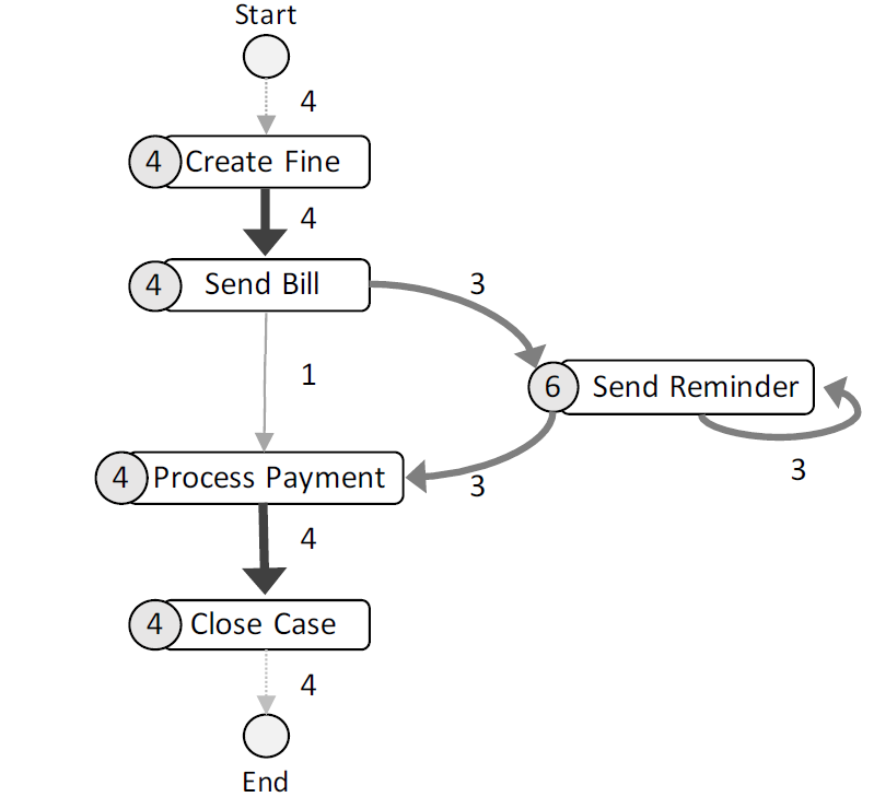
Directly follows graph

Figure 1. Event log and its corresponding process map

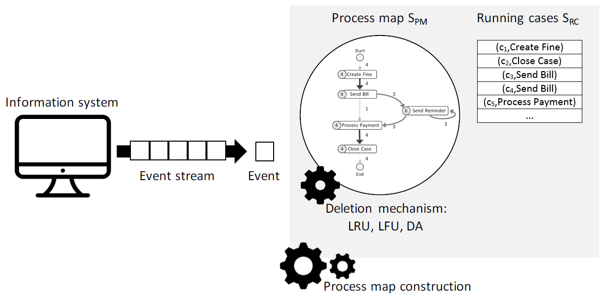
Figure 2. Overview of the proposed approach

3. Approach

This section presents the main contribution of the paper. The first subsection introduces the fundamental notions of event logs and process maps, while the second subsection presents a novel technique for the discovery of process maps from event streams.

3.1. Preliminaries

Event logs record the execution of activities in a business process. Every execution of a process constitutes a case and produces a sequence of activity occurrences called a trace. The activity occurrences are referred to as events and can have several attributes. Here, we assume that events are equipped with only three attributes: case id, activity name and timestamp. For instance, Fig. 1 shows an event log (left-hand side) with 5 activities and 22 events.

Definition 3.1 (Event).

Let $\mathcal{A}$ be the set of all activity names, $\mathcal{C}$ be the set of case identifiers and $\mathcal{T}$ be the set of timestamps of an event log. An event is a tuple $e=\langle A,C,T\rangle\in\mathcal{A}\times\mathcal{C}\times\mathcal{T}$ and represents the occurrence of activity $A$ at time $T$ in the case with id $C$. The set of all possible events is denoted as $\mathcal{E}$.

Given an event $e=\langle A,C,T\rangle$, we refer to its activity, case and timestamp as $e|_{A}=A$, $e|_{C}=C$ and $e|_{T}=T$, respectively. The timestamps reflect the order of execution of the events. The bounded sequence of ordered events (w.r.t. timestamps) occurring within the same case is called a trace; whereas, an unbounded sequence of events belonging to different cases is called an event stream.

Definition 3.2 (Trace and event stream).

Let $\mathcal{E}$ be the set of events of an event log. A trace is a bounded sequence of events $\sigma=\langle e_{1},\dots,e_{n}\rangle$, such that $e_{x}|_{T}<e_{y}|_{T}$ and $e_{x}|_{C}=e_{y}|_{C}$, for any $1\leq x<y\leq n$ and $e_{x},e_{y}\in\mathcal{E}$. An event stream is an unbounded sequence of events $\sigma=\langle e_{1},\dots\rangle$ with the same order among the events as in a trace, i.e., $e_{x}|_{T}<e_{y}|_{T}$, for any $1\leq x<y$.

Two events $e_{x}$, $e_{y}$ are said to be in a directly follows relation if they belong to the same case and they occurred consecutively.

Definition 3.3 (Directly follows relations).

Let $\sigma=\langle e_{1},e_{2},\allowbreak\dots\rangle$ be a sequence of events, either a trace or an event stream. A pair of events $e_{x}$ and $e_{y}$ are in a directly follows relation, denoted as $e_{x}\Rightarrow e_{y}$, if $e_{x}|_{C}=e_{y}|_{C}$, $e_{x}|_{T}<e_{y}|_{T}$ and $\nexists e_{z}\in\mathcal{E}:e_{z}|_{C}=e_{x}|_{C}=e_{y}|_{C}~{}\land~{}e_{x}|_{T}<e_{z}|_{T}<e_{y}|_{T}$, for any $1\leq x,y,z$.

Trace $\langle Create\ \allowbreak Fine,~{}\allowbreak Send\ \allowbreak Bill,~{}\allowbreak Process\ \allowbreak Payment,\allowbreak Close\ \allowbreak Case\rangle$ contains three directly follows relations: $Create\ \allowbreak Fine\allowbreak\Rightarrow\allowbreak Send\ \allowbreak Bill$, $Send\ \allowbreak Bill\allowbreak\Rightarrow\allowbreak Process\ \allowbreak Payment$ and $Process\ \allowbreak Payment\allowbreak\Rightarrow\allowbreak Close\ Case$.

The directly follows relations implicitly represented in a set of traces or an event stream can be abstracted into a directly follows graph, also called a process map. This abstraction is used by some process mining algorithms, such as the Heuristic Miner (Weijters et al., 2006), as a baseline for the discovery of other types of models, e.g., models in BPMN notation. Intuitively, a directly follows graph is a graph where nodes represent activities, arcs represent directly follows relations, and every node and every arc is annotated with its frequency (number of times the activity/relation has been observed in the log).

Definition 3.4 (Directly follows graph).

Let $\mathcal{A}$ be the set of all activity names of an event log. A directly follows graph is a tuple $S_{PM}=\langle V,E,\gamma\rangle$, where $V\subseteq\mathcal{A}$ is a set of nodes representing activities, $E\subseteq V\times V$ is a set of arcs representing directly follows relations between activities, and $\gamma:V\cup E\rightarrow\mathbb{N}_{0}$ is a function associating nodes and arcs to frequencies.

Figure 1 displays an event log and its representation as a directly follows graph aside, nodes and arcs are annotated with their frequency, and a start and an end node were inserted to denote start and end of traces. In this graphical representation, the thickness of the arcs vary depending on their frequency, the thicker the arrow the higher the frequency.

3.2. Online process map discovery

This subsection presents a novel technique for discovering process maps from event streams. The general idea is to maintain two memory partitions: $S_{PM}$, which is allocated to store the process map itself, and $S_{RC}$, which keeps track of the observed cases in the event stream. Then, for every event $e=\langle A,C,T\rangle$ observed in the event stream, our technique will seek for the last observed event $e^{\prime}$ in $S_{RC}$ with the same case id $c$; if $e^{\prime}$ exists then a new directly follows relation $e^{\prime}|_{A}\Rightarrow e|_{A}$ is either created (if it does not exist already) or updated (if it exists) by increasing its frequency; finally $e$ is stored in $S_{RC}$. Note that every observed event triggers the update of the process map, either by creating a new node (if the activity has not been observed), or by creating a new arc, or by increasing the frequency of a node and/or an arc. An overview of the proposed technique is displayed in Fig. 2

The storage of all the information read from an event stream can result impractical since new events, relations and cases can continuously emerge. In order to cope with possible memory limitations, $S_{RC}$ stores only the last observed event for every case; note that this information is sufficient to discover the directly follows relations. Furthermore, a memory size $B_{PM}$ and $B_{RC}$ – hereinafter referred to as budgets – can be associated to each partition $S_{PM}$ and $S_{RC}$, respectively. Both budgets determine the amount of objects (activities, relations and cases) that can be allocated for the process map and for the running cases. Thus, in order to have a lossless representation of a process map from an event stream with activity names in $\mathcal{A}$, it is necessary to allocate enough space for storing a graph with $N$ nodes, where $N$ is the number of distinct activity names in $\mathcal{A}$, and all possible arcs between every pair of activities (including self-loops). Thus, for a lossless representation, the budget $B_{PM}$ has to be equal to:

(1) $$B_{PM}=\frac{N(N+1)}{2}+N.$$

Intuitively, Equation 1 counts the number of arcs in a clique, plus the self-loops and the number of nodes. However, if the budget $B_{PM}$ is not large enough to store a lossless process map representation, then once $S_{PM}$ is full, some elements need to be deleted to give place to new relations or activities observed in the stream. The budget $B_{RC}$ controls the amount of running instances that can be stored in $S_{RC}$ and, similarly to $S_{PM}$, once it is full then some elements need to be deleted in order to memorize new observed cases. Both partitions can be maintained separately, have distinct sizes and have different deletion mechanisms.

We propose three deletion mechanisms for $S_{PM}$ based on well-known concepts from cache memory management. Cache replacement policies identify elements to be cached or deleted in HTTP proxies to reduce network traffic and response time (Arlitt et al., 2000). We adapt the three following cache replacement policies for the deletion mechanism for $S_{PM}$:

• Least Recently Used (LRU) deletes the elements in the cache that have not been used for the longest period of time. From the basics of temporal locality, the elements that have been referenced recently will be likely referenced in the near future. This policy works well when there is a high temporal locality of references in the workload. In our context, relations and activities read from the event stream are annotated with the “last seen index” attribute to keep track of their recency.

• Least Frequently Used (LFU) removes the element with the smallest frequency of occurrence. In our context, no additional attributes are required since the frequency of the relations and activities is already stored as part of the directly follows graph through the use of $\gamma$.

• LFU with Dynamic Aging (LFU-DA) removes the element with the highest value given by $K_{T}=\gamma(t)+L$, where $t$ is either a relation or an activity and $L$ is a dynamic aging factor. Initially, $L$ is set to 0, thus the policy is the same as LFU before the first deletion. However, once an element $t^{\prime}$ is deleted, $L$ is set to $K_{t^{\prime}}$.

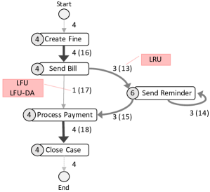
Figure 3. Relations to be deleted

Once $S_{PM}$ is full and new information needs to be stored, the elements selected by the chosen policy are deleted from the partition $S_{PM}$. The deletion procedure considers two cases: (i) if the element is a relation, then it is simply removed, but (ii) if it is an activity, then the activity and all the relations associated to it are removed. $S_{PM}$ is subdivided into $E$ and $V$ for storing the relations and the activities, respectively. With abuse of notation, let $|E|$ (resp. $|V|$) denote the size of the partition for the relations (resp. for the activities), thus $B_{PM}=|E|+|V|$.

input : Event stream $ES$, $B_{PM}$ and $B_{RC}$ 1 $E,V,S_{RC}\leftarrow\emptyset$   $idx\leftarrow 1$ // LRU   $L\leftarrow 1$ // LFU-DA 2 3Loop   4       $e=\langle A,C,T\rangle\leftarrow observe(ES)\;$ 5       if $A\in V$ then 6             $\gamma(A)=\gamma(A)+1$                update $lastSeenIdx(A)$ // LRU 7             8      else 9             if $B_{PM}=|E|+|V|$ then 10                   $deletionMechanism()$                      update $L$ // LFU-DA 11                   12             end if               $V\leftarrow V\cup\{(A,idx)\}$ // LRU                $V\leftarrow V\cup\{A\}$ // LFU                $V\leftarrow V\cup\{(A,L)\}$ // LFU-DA 13             14       end if 15       16      if $C\in S_{RC}$ then 17             $rc\leftarrow\langle C,A^{\prime}\rangle\in S_{RC}$ 18             if $r=(A^{\prime},A)\in E$ then 19                   $\gamma(r)=\gamma(r)+1$                      update $lastSeenIdx(r)$ // LRU 20                   21            else 22                   if $B_{PM}=|E|+|V|$ then 23                         $deletionMechanism()$                            update $L$ // LFU-DA 24                         25                   end if                     $E\leftarrow E\cup\{(r,idx)\}$ // LRU                      $E\leftarrow E\cup\{r\}$ // LFU                      $E\leftarrow E\cup\{(r,L)\}$ // LFU-DA 26                   27             end if 28            $S_{RC}\leftarrow(S_{RC}\backslash\{rc\})\cup\{(c,A)\}$ 29            if $isExpired(c)$ then 30                   $S_{RC}\leftarrow S_{RC}\backslash\{(C,A^{\prime\prime})\}$ for any $A^{\prime\prime}$ 31             end if 32             33      else 34             $S_{RC}\leftarrow S_{RC}\cup\{(c,A)\}$ 35       end if 36      $idx\leftarrow idx+1$ 37 EndLoop Algorithm 1 Process map construction		input : $E,V$ 1 2$min_{a}\leftarrow min\{idx|(A,idx)\in V\}$ 3 $min_{r}\leftarrow min\{idx|(r,idx)\in E\}$ 4 if $min_{a}>min_{r}$ then 5       $E\leftarrow E\backslash\{(r,idx)\}$ 6else 7       $V\leftarrow V\backslash\{(A,idx)\}$ 8       for $((A^{\prime},A^{\prime\prime}),idx)\in E$ such that $A^{\prime}=A$ or $A^{\prime\prime}=A$ do 9             $E\leftarrow E\backslash\{(r,idx)\}$ 10       end for 11       12 end if Algorithm 2 Deletion mechanism LRU
		input : $E,V$ 1 2$min_{a}\leftarrow min\{\gamma(A)|A\in V\}$ 3 $min_{r}\leftarrow min\{\gamma(r)|r\in E\}$ 4 if $min_{a}>min_{r}$ then 5       $E\leftarrow E\backslash\{r\}$ 6else 7       $V\leftarrow V\backslash\{A\}$ 8       for $(A^{\prime},A^{\prime\prime})\in E$ such that $A^{\prime}=A$ or $A^{\prime\prime}=A$ do 9             $E\leftarrow E\backslash\{r\}$ 10       end for 11       12 end if Algorithm 3 Deletion mechanism LFU
		input : $E,V$ 1 2$min_{a}\leftarrow min\{\gamma(A)+L|(A,L)\in V\}$ 3 $min_{r}\leftarrow min\{\gamma(r)+L|(r,L)\in E\}$ 4 if $min_{a}>min_{r}$ then 5       $E\leftarrow E\backslash\{(r,L)\}$ 6else 7       $V\leftarrow V\backslash\{(A,L)\}$ 8       for $((A^{\prime},A^{\prime\prime}),L)\in E$ such that $A^{\prime}=A$ or $A^{\prime\prime}=A$ do 9             $E\leftarrow E\backslash\{(r,L)\}$ 10       end for 11       12 end if Algorithm 4 Deletion mechanism LFU-DA

Table 1. Algorithms

Consider the directly follows graph in Fig. 3, where every arc is annotated with its frequency and its “last seen index” in parenthesis. If LRU is chosen as the deletion mechanism, then the arc representing $Send\ Bill\Rightarrow Send\ Reminder$ is deleted since this relation is the least recently observed. On the other hand, if LFU is chosen, then the relation to remove is $Send\ Bill\Rightarrow Process\ Payment$ (and similarly for LFU-DA during the first deletion), since this relation is the least frequent one.

The deletion mechanism for $S_{RC}$ imposes different challenges than the one used for $S_{PM}$. The information kept in $S_{RC}$ is necessary to compute the directly follows relations, but, if the amount of cases is unknown, then no ideal budget $B_{RC}$ can be defined. Clearly, if the end of every case is known (last event of every trace) then an entry can be eliminated from $S_{RC}$ once the corresponding case is ended. Nevertheless, other strategies can be implemented based on time or resources, e.g., a case can be deleted from $S_{RC}$ if it has been running longer than a given threshold. The size of $S_{RC}$ is denoted as $|S_{RC}|$.

Algorithm 1 shows the procedure to construct the process map from an event stream. The highlighted lines in Algorithm 1 apply depending on the chosen deletion mechanism: LRU, LFU or LFU-DA (see the annotation on each highlighted line). The algorithm starts by reading an incoming event $e$ from the event stream (method $observe$ at line 5). If the activity of $e$ is already in $V$, then its frequency as well as its index (in the case of LRU) are updated (lines 6-8); otherwise, if the activity is not contained in $V$ then it is necessary to check whether there is enough space to store the new activity (line 10). If the partition $S_{PM}$ is full then one of the deletion mechanisms is applied: LRU (Alg. 2), LFU (Alg. 3), or LFU-DA (Alg. 4). The procedure continues by inserting the activity into $V$ (lines 14-16). If the event belongs to a case $c$ that has been observed previously and the directly follows relation between the activities of the last observed event in $c$ and of the new event $e$ is present in $E$, then its frequency and index are updated (lines 20-22). Otherwise, the algorithm proceeds by inserting the relation in $E$ (lines 28-30), after applying the deletion mechanism if necessary (lines 24-27). The activity of the observed event is inserted into $S_{RC}$ (line 32). Finally, if the case is expired (e.g., event $e$ is the end event of the case), then it is deleted from $S_{RC}$.

Algorithms 2-4 show the deletion mechanisms. All these mechanisms work in a similar way: first, they detect the elements to delete (depending on the recency, frequency or frequency with dynamic aging) and, then, they remove them from $V$ or $E$. Note that if the element to be deleted is an activity, then all the relations involving that activity are removed as well.

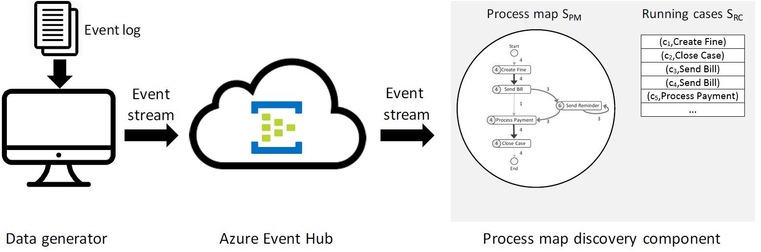
Figure 4. Evaluation setup

Dataset	# Traces	# Events	# Events per trace (Avg.)	# Activities
BPIC 2016	660,270	7,174,934	10.86	600
BPIC 2018	43,809	2,514,266	57.39	170
University log	174,842	2,099,835	12.00	310

Table 2. Datasets

Technique	Activity	Relation	Case
LCB	3	4	4
LRU	3	4	3
LFU	2	3	3
LFU-DA	3	4	3

Table 3. Words needed to store activities, relations and cases

4. Evaluation

Our approach for the discovery of directly follows graphs has been implemented in .NET and experimentally integrated into the process mining tool Minit. The tool reads an event stream from a publish-subscribe service and updates an in-memory directly follows graph whenever an event is read. In our evaluation, we use Azure event hub, a highly scalable publish-subscribe service, to play the role of a reliable channel between the originator of the event stream (customer) and the process map discovery component. In order to simulate a customer, a data generator component was also implemented in .NET. The data generator reads a log and streams every event to the publish-subscribe service. The evaluation setup is depicted in Fig. 4.

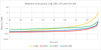
(a) BPIC 2016

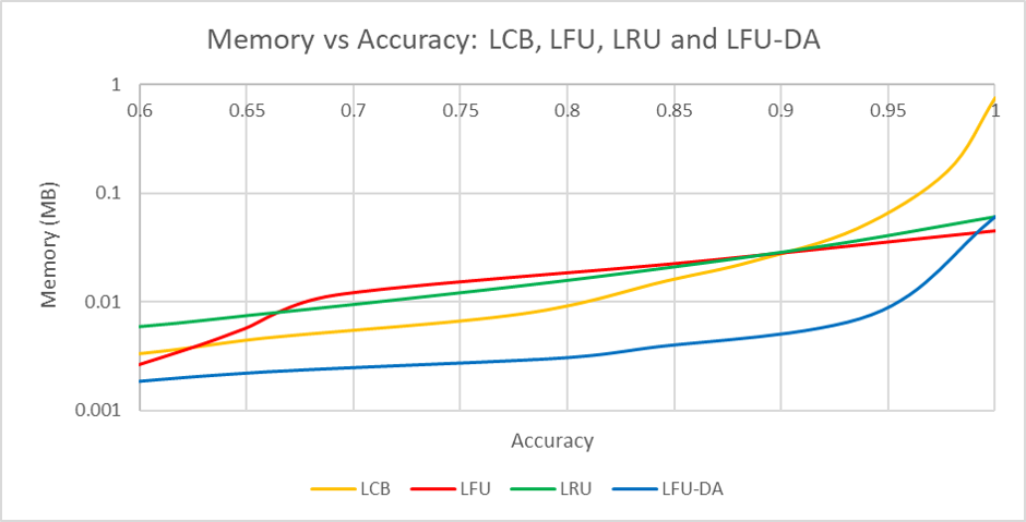
(b) BPIC 2018

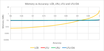
(c) University log

Figure 5. Memory vs. Accuracy

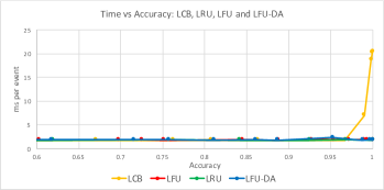
(a) BPIC 2016

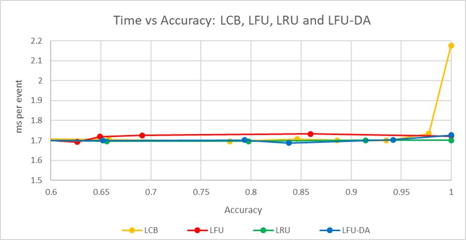
(b) BPIC 2018

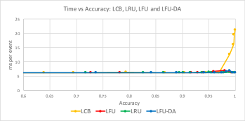
(c) University log

Figure 6. Time vs. Accuracy

We used three large event logs in our evaluation: BPI Challenge (BPIC) 2016, BPIC 2018, and a University log. BPIC 2016 is a publicly available log pertaining to the process that customers go through in a Dutch administrative authority to manage unemployment benefits. The data was collected over a period of eight months. The process considered in the BPIC 2018 covers the handling of applications for EU direct payments (basic incomes decoupled from production) for German farmers from the European Agricultural Guarantee Fund. The University log refers to a process from an accounting department of an Italian University. The number of traces, number of events, average number of events per trace, and number of distinct activities for each of these logs are shown in Table 2.

We compare the different deletion strategies in our approach (LRU, LFU and LFU-DA) against Lossy Counting with Budget (LCB) (Burattin et al., 2014b), which is, to the best of our knowledge, the most efficient online process discovery technique described in the literature. The comparison of the different approaches is done in terms of time per event (ms) and memory consumption required to obtain different levels of accuracy.

Accuracy evaluates the similarity between the exact directly follows graph, which is discovered from the entire event log, and the one discovered by each of the online techniques (LCB, LRU, LFU and LFU-DA). Specifically, accuracy counts the differences in frequencies between the relations in both directly follows graphs. If a relation is not present in either of the graphs, then its frequency is treated as 0; whereas, if an activity is missing in the directly follows graph discovered by an online technique (which exists in the complete graph), then this activity and all the relations it is involved in are added with a frequency of 0. The sum of all differences in frequencies constitutes the Loss, whereas the sum of all frequencies in the complete graph constitutes the Total frequency. Then, the accuracy of a graph created by an online technique is computed with the following formula:

(2) $$A=1-\frac{Loss}{Total\ frequency}.$$

Memory consumption shows the amount of memory used during the discovery of the directly follows graph. It is measured in terms of memory words, which refer to a fixed-size unit of memory. The number of words required by each technique to store an activity, a relation and a case is displayed in Table 3. The total memory consumption for a technique is computed with the formula:

(3) $$M=M(activity)\times|V|+M(relation)\times|E|+M(case)\times|S_{RC}|,$$

where $M(activity)$, $M(relation)$ and $M(case)$ are the number of words required to store activities, relations and cases (see Table 3).

In Fig. 5, we compare LCB with the three different deletion mechanisms of our approach: LRU, LFU and LFU-DA by evaluating the memory consumption required to obtain different levels of accuracy. In all the approaches, we assume that the end event for each case is known. Thus, as mentioned in the previous section, once the end event of a case is read from the stream, the case is deleted from $S_{RC}$. The memory is reported in terms of MB (a word is equal to 4 bytes) and we use logarithmic scale on the Memory axis.

In order to obtain a lossless directly follows graph for BPIC 2016 (Fig. 5a), the memory required is LCB = 10.76 MB, LRU = 0.2 MB, LFU = 0.15 MB, and LFU-DA = 0.2 MB. Therefore, LCB requires a considerably larger amount of memory (two orders of magnitude higher) than the three variants of our approach. The amount of memory used by LCB starts to be higher than the amount of memory required by LFU and LFU-DA when the accuracy exceeds 0.65, while in the case of LRU, it happens when the accuracy exceeds 0.85. The memory required for a lossless directly follows graph for BPIC 2018 (Fig. 5b) is LCB = 0.76 MB, LRU = 0.07 MB, LFU = 0.06 MB, and LFU-DA = 0.07 MB. Also in this case, LCB requires a larger amount of memory (one order of magnitude higher) than our approach. In this case, the amount of memory used by LCB is always higher than the amount of memory required by LFU-DA, whereas the amount of memory used by LCB starts to be higher than the amount of memory required by LRU and LFU when the accuracy exceeds 0.9. The results for the University log (Fig. 5c) show that LCB requires a larger amount of memory for an accuracy higher than 0.9, while the amount of memory is very similar for all variants of our approach. The amount of memory for a lossless directly follows graph is LCB = 2.82 MB, LRU = 0.10 MB, LFU = 0.10 MB, and LFU-DA = 0.10 MB, and LCB uses one order of magnitude more memory than our approach.

Figure 6 reports time performance (ms per event) vs. accuracy. For BPIC 2016 (Fig. 6a), LCB takes significantly longer when the accuracy approaches 1.0, while our approach performs in a similar way across its different variants. Figure 6b shows the results for BPIC 2018. We can see that, for this log, LRU, LFU and LFU-DA take around 1.7 ms per event when the accuracy is 1.0, while LCB requires 2.19 ms. The results for the University log are displayed in Fig. 6c. Here, LRU, LFU and LFU-DA take 6.22 ms per event when the accuracy is 1.0, while LCB requires 21.29 ms. The variations in time in Fig. 6 show that, when the end event of each case is known, the deletion mechanisms in all the variants of our approach are more efficient than the one in LCB.

5. Conclusion

This paper proposes an approach for the online discovery of process maps from a stream of events. The approach relies on three cache replacement policies to maintain an up-to-date in-memory representation of the process map, which is updated whenever a new process event or behavioral relation between process events is observed from the stream. The evaluation on real-life datasets shows that our approach outperforms the state of the art, in terms amount of memory and time per event. The performance is comparable if the last event of each case is not known. In addition, the approach provides a clear way to control the accuracy of the resulting process map.

As future work, we plan to use cache replacement policies for the online discovery of other types of process models such as declarative models and social networks of the interactions among process participants. We also plan to discover process maps that consider other metrics along with the frequency of the directly follows relations, such as the time difference between adjacent events, as a means to evaluate the performance of the underlying business process.

References

- (1)
- Agrawal et al. (1998) Rakesh Agrawal, Dimitrios Gunopulos, and Frank Leymann. 1998. Mining Process Models from Workflow Logs. In Advances in Database Technology - EDBT’98, 6th International Conference on Extending Database Technology, Valencia, Spain, March 23-27, 1998, Proceedings. 469–483. https://doi.org/10.1007/BFb0101003
- Arlitt et al. (2000) Martin F. Arlitt, Ludmila Cherkasova, John Dilley, Rich Friedrich, and Tai Jin. 2000. Evaluating content management techniques for Web proxy caches. SIGMETRICS Performance Evaluation Review 27, 4 (2000), 3–11. https://doi.org/10.1145/346000.346003
- Augusto et al. (2017) Adriano Augusto, Raffaele Conforti, Marlon Dumas, Marcello La Rosa, Fabrizio Maria Maggi, Andrea Marrella, Massimo Mecella, and Allar Soo. 2017. Automated Discovery of Process Models from Event Logs: Review and Benchmark. ArXiv CoRR (2017).
- Bose (2012) R.P. Jagadeesh Chandra Bose. 2012. Process Mining in the Large: Preprocessing, Discovery, and Diagnostics. Ph.D. Dissertation. Eindhoven University of Technology.
- Burattin et al. (2014a) Andrea Burattin, Marta Cimitile, and Fabrizio Maria Maggi. 2014a. Lights, Camera, Action! Business Process Movies for Online Process Discovery. In Business Process Management Workshops - BPM 2014 International Workshops, Eindhoven, The Netherlands, September 7-8, 2014, Revised Papers. 408–419. https://doi.org/10.1007/978-3-319-15895-2_34
- Burattin et al. (2015) Andrea Burattin, Marta Cimitile, Fabrizio Maria Maggi, and Alessandro Sperduti. 2015. Online Discovery of Declarative Process Models from Event Streams. IEEE Trans. Services Computing 8, 6 (2015), 833–846. https://doi.org/10.1109/TSC.2015.2459703
- Burattin et al. (2012) Andrea Burattin, Alessandro Sperduti, and Wil M. P. van der Aalst. 2012. Heuristics Miners for Streaming Event Data. ArXiv CoRR (Dec. 2012). arXiv:1212.6383 http://arxiv.org/abs/1212.6383
- Burattin et al. (2014b) Andrea Burattin, Alessandro Sperduti, and Wil M. P. van der Aalst. 2014b. Control-flow discovery from event streams. In Proceedings of the IEEE Congress on Evolutionary Computation, CEC 2014, Beijing, China, July 6-11, 2014. 2420–2427. https://doi.org/10.1109/CEC.2014.6900341
- Da San Martino et al. (2013) Giovanni Da San Martino, Nicolò Navarin, and Alessandro Sperduti. 2013. A Lossy Counting Based Approach for Learning on Streams of Graphs on a Budget. In IJCAI 2013, Proceedings of the 23rd International Joint Conference on Artificial Intelligence, Beijing, China, August 3-9, 2013. 1294–1301. http://www.aaai.org/ocs/index.php/IJCAI/IJCAI13/paper/view/6699
- De Weerdt et al. (2012) Jochen De Weerdt, Manu De Backer, Jan Vanthienen, and Bart Baesens. 2012. A multi-dimensional quality assessment of state-of-the-art process discovery algorithms using real-life event logs. Inf. Syst. 37, 7 (2012), 654–676. https://doi.org/10.1016/j.is.2012.02.004
- Hassani et al. (2015) Marwan Hassani, Sergio Siccha, Florian Richter, and Thomas Seidl. 2015. Efficient Process Discovery From Event Streams Using Sequential Pattern Mining. In IEEE Symposium Series on Computational Intelligence, SSCI 2015, Cape Town, South Africa, December 7-10, 2015. 1366–1373. https://doi.org/10.1109/SSCI.2015.195
- Kindler et al. (2005) Ekkart Kindler, Vladimir A. Rubin, and Wilhelm Schäfer. 2005. Incremental Workflow Mining Based on Document Versioning Information. In Unifying the Software Process Spectrum, International Software Process Workshop, SPW 2005, Beijing, China, May 25-27, 2005, Revised Selected Papers. 287–301. https://doi.org/10.1007/11608035_25
- Kindler et al. (2006) Ekkart Kindler, Vladimir A. Rubin, and Wilhelm Schäfer. 2006. Incremental Workflow Mining for Process Flexibility. In Proceedings of the CAISE*06 Workshop on Business Process Modelling, Development, and Support BPMDS ’06, Luxemburg, June 5-9, 2006. http://ceur-ws.org/Vol-236/paper12.pdf
- Maaradji et al. (2015) Abderrahmane Maaradji, Marlon Dumas, Marcello La Rosa, and Alireza Ostovar. 2015. Fast and Accurate Business Process Drift Detection. In Business Process Management - 13th International Conference, BPM 2015, Innsbruck, Austria, August 31 - September 3, 2015, Proceedings. 406–422. https://doi.org/10.1007/978-3-319-23063-4_27
- Maggi et al. (2013) Fabrizio Maria Maggi, Andrea Burattin, Marta Cimitile, and Alessandro Sperduti. 2013. Online Process Discovery to Detect Concept Drifts in LTL-Based Declarative Process Models. In On the Move to Meaningful Internet Systems: OTM 2013 Conferences - Confederated International Conferences: CoopIS, DOA-Trusted Cloud, and ODBASE 2013, Graz, Austria, September 9-13, 2013. Proceedings. 94–111. https://doi.org/10.1007/978-3-642-41030-7_7
- Maggi et al. (2012) Fabrizio Maria Maggi, Marco Montali, and Wil M. P. van der Aalst. 2012. An Operational Decision Support Framework for Monitoring Business Constraints. In Fundamental Approaches to Software Engineering - 15th International Conference, FASE 2012, Held as Part of the European Joint Conferences on Theory and Practice of Software, ETAPS 2012, Tallinn, Estonia, March 24 - April 1, 2012. Proceedings. 146–162.
- Maggi and Westergaard (2017) Fabrizio Maria Maggi and Michael Westergaard. 2017. Designing software for operational decision support through coloured Petri nets. Enterprise IS 11, 5 (2017), 576–596.
- Manku and Motwani (2012) Gurmeet Singh Manku and Rajeev Motwani. 2012. Approximate Frequency Counts over Data Streams. PVLDB 5, 12 (2012), 1699. http://vldb.org/pvldb/vol5/p1699_gurmeetsinghmanku_vldb2012.pdf
- Ostovar et al. (2017) Alireza Ostovar, Abderrahmane Maaradji, Marcello La Rosa, and Arthur H. M. ter Hofstede. 2017. Characterizing Drift from Event Streams of Business Processes. In Advanced Information Systems Engineering - 29th International Conference, CAiSE 2017, Essen, Germany, June 12-16, 2017, Proceedings. 210–228. https://doi.org/10.1007/978-3-319-59536-8_14
- Ostovar et al. (2016) Alireza Ostovar, Abderrahmane Maaradji, Marcello La Rosa, Arthur H. M. ter Hofstede, and Boudewijn F. van Dongen. 2016. Detecting Drift from Event Streams of Unpredictable Business Processes. In Conceptual Modeling - 35th International Conference, ER 2016, Gifu, Japan, November 14-17, 2016, Proceedings. 330–346. https://doi.org/10.1007/978-3-319-46397-1_26
- Pesic et al. (2007) Maja Pesic, Helen Schonenberg, and Wil M. P. van der Aalst. 2007. DECLARE: Full Support for Loosely-Structured Processes. In 11th IEEE International Enterprise Distributed Object Computing Conference (EDOC 2007), 15-19 October 2007, Annapolis, Maryland, USA. 287–300. https://doi.org/10.1109/EDOC.2007.14
- Sharp and McDermott (2008) Alec Sharp and Patrick McDermott. 2008. Workflow Modeling: Tools for Process Improvement and Application Development. Artech House Publishers. 449 pages.
- van der Aalst (2015) Wil M. P. van der Aalst. 2015. Process Mining: Data Science in Action, second edition. Springer.
- van Zelst et al. (2018) S. J. van Zelst, B. F. van Dongen, and W. M. P. van der Aalst. 2018. Event stream-based process discovery using abstract representations. Knowledge and Information Systems 54, 2 (2018), 407–435. https://doi.org/10.1007/s10115-017-1060-2
- Weijters et al. (2006) Ton Weijters, Wil M. P. van der Aalst, and A. K. Alves De Medeiros. 2006. Process mining with the heuristics miner-algorithm. TU/e, Tech. Rep. 166 (2006), 1–34.
- Westergaard and Maggi (2011) Michael Westergaard and Fabrizio Maria Maggi. 2011. Modeling and Verification of a Protocol for Operational Support Using Coloured Petri Nets. In Applications and Theory of Petri Nets - 32nd International Conference, PETRI NETS 2011, Newcastle, UK, June 20-24, 2011. Proceedings. 169–188.