Solving Pooling Problems by LP and SOCP Relaxations and Rescheduling Methods

Abstract

The pooling problem is an important industrial problem in the class of network flow problems for allocating gas flow in pipeline transportation networks. For P-formulation of the pooling problem with time discretization, we propose second order cone programming (SOCP) and linear programming (LP) relaxations and prove that they obtain the same optimal value as the semidefinite programming relaxation. The equivalence among the optimal values of the three relaxations is also computationally shown. Moreover, a rescheduling method is proposed to efficiently refine the solution obtained by the SOCP or LP relaxation. The efficiency of the SOCP and the LP relaxation and the proposed rescheduling method is illustrated with numerical results on the test instances from the work of Nishi in 2010, some large instances, and Foulds 3, 4, 5 test problems.

Key words. Pooling problem, Semidefinite relaxation, Second order cone relaxation, Linear programming relaxation, Rescheduling method, Computational efficiency.

AMS Classification. 90C20, 90C22, 90C25, 90C26.

1 Introduction

The pooling problem is a network flow problem for allocating gas flow in pipeline transportation networks with minimum cost. It arises from applications in the petroleum industry. Networks of the pooling problem have three types of nodes: sources, blending tanks called pools and plants. Gas flows from the sources are blended in the blending tanks and plants to produce the desired final products. To model such blending, the pooling problem is formulated as bilinear nonconvex optimization problems, thus nonconvex quadratically constrained quadratic problems (QCQPs) [11].

The pooling problem has been studied in two main formulations, the P-formulation [11] and Q-formulation [9]. Difficulties of solving the pooling problem arise from the existence of pipeline constraints formulated with binary variables and the blending process represented as nonlinear constraints. The resulting problem is a mixed-integer nonlinear program known as NP-hard [6]. Various solution methods including approximating heuristics, linear programming relaxations, decomposition techniques have been proposed for these formulations. In particular, successive linear relaxations [10, 14] approximate the pooling problem based on a first-order Taylor expansion. Another popular approach is branch-and-bound algorithms which have been implemented to solve large-scale problems [6].

While conic relaxations methods including semidefinite programming (SDP), second order cone (SOCP) and linear programming (LP) relaxations of general nonconvex QCQPs have been widely used to approximate the optimal values of the problems, they have not studied extensively for the pooling problem. In fact, no literature on SOCP and LP relaxations of the pooling problem could be found to the authors’ best knowledge. SDP relaxations of the pooling problem were studied in [16, 22]. SDP relaxations of nonconvex QCQPs are known to provide tighter bounds for the optimal value than SOCP and LP relaxations, however, solving SDP relaxations by the primal-dual interior-point methods [17, 18, 20, 21] is computationally expensive. Thus, the size of the problems that can be solved by SDP relaxations remains very limited. From a computational perspective, SOCP and LP relaxations are more efficient than SDP relaxations, as a result, large-sized problems can be solved by SOCP and LP relaxations [12].

The main purpose of this paper is to propose an efficient computational method that employs LP and SOCP relaxations and a rescheduling method for the P-formulation of the pooling problem with time discretization. The LP relaxation of nonconvex QCQPs in this paper is different from the linear programming based on a first-order Taylor expansion [10, 14]. Let $\zeta^{*}$ be the optimal value of a general nonconvex QCQP that minimizes the objective function. Among $\zeta^{*}$ and the optimal values of SDP, SOCP and LP relaxations of the QCQP, we have the following relationship:

$$\zeta_{LP}^{*}\leq\zeta_{SOCP}^{*}\leq\zeta_{SDP}^{*}\leq\zeta^{*}.$$

LP relaxations are known to be most efficient and SDP relaxations most time-consuming among the three relaxations for solving general QCQPs. For our formulation of the pooling problem, we prove that the SDP, SOCP and LP relaxations provide the equivalent optimal value:

$$\zeta_{LP}^{*}=\zeta_{SOCP}^{*}=\zeta_{SDP}^{*}\leq\zeta^{*}.$$ (1)

More precisely, the LP relaxation can be used to obtain the same quality of the optimal value as that of the SDP relaxation with much less computational efforts. Thus, larger pooling problems can be handled with the LP relaxation. We theoretically prove the equivalence (1) and present the computational results that support (1). Moreover, we demonstrate that (1) holds for other formulations of the pooling problem where bilinear terms appear with no squared terms of the variables. The LP relaxation presented in this paper can be used to efficiently solve different formulations of the pooling problem.

The solution obtained by the LP, SOCP and SDP relaxations of the pooling problem should be refined to satisfy all the constraints of the original problem. For this issue, Nishi [16] proposed a method that solves a mixed-integer linear program using the solution obtained by the SDP relaxation, then applies an iterative procedure for the nonlinear terms, and finally uses a nonlinear program solver to attain a local optimal solution. In the three steps of his method, the nonlinear program solver particularly takes long computational time, making the entire method very time-consuming. To reduce the computational burden caused by applying a nonlinear program solver, we propose a rescheduling method which successively updates a local optimal solution by applying the SOCP or LP relaxation to partial time steps of the entire time discretization. The proposed technique significantly increases the computational efficiency of the entire method, which enables us to solve large pooling problems. For one test instance with 1228 variables, the rescheduling method reduced the computational time for a general nonlinear solver by 1/60.

This paper is organized as follows: Section 2 briefly describes the pooling problem. In Section 3, we illustrate SDP, SOCP, and LP relaxations of the general nonconvex QCQPs. Section 4 includes the proof of the optimal values on the three relaxations of our formulation of the pooling problem and discusses how the result can be applied to other formulations of the pooling problem. In Section 5, we describe the proposed rescheduling methods in detail. Section 6 presents numerical results on the test problems in [16], some large instances and Foulds 3, 4, 5. We conclude in Section 7.

2 The pooling problem

We first describe the formulation of the pooling problem with time discretization in [16], then present our formulation.

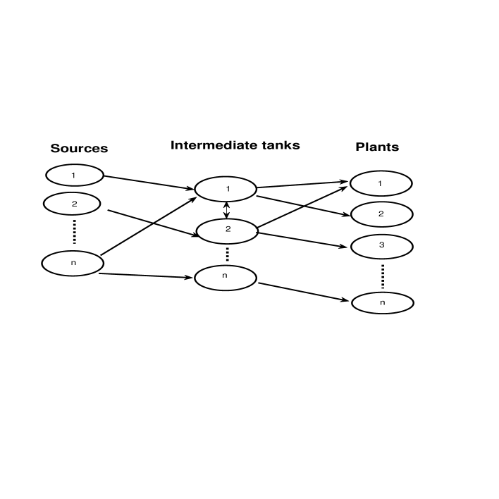
Figure 1: Overview

2.1 Notation

Let $M_{S}$, $M_{I}$ and $M_{P}$ denote the numbers of sources, intermediate tanks, and plants, respectively. We also let $V$ be the set of all nodes. The sets of sources, intermediate tanks and plants are denoted by $V_{S}$, $V_{I}$ and $V_{P}$, respectively, as follows:

$$V_{S} =\{1,2,\dots,M_{S}\},\ \ V_{I}=\{M_{S}+1,\dots,M_{S}+M_{I}\},\$$

$$V_{P} =\{M_{S}+M_{I}+1,\dots,M_{S}+M_{I}+M_{P}\},\ V=V_{S}\cup V_{I}\cup V_{P}.$$

The arrows in Figure 1 mean pipelines. The pipeline between $i$ and $j\in V$ is denoted as $(i,j)$, and the set of pipelines is denoted as $A$. Furthermore, for the $i$th node, the set of entering nodes and that of leaving nodes are denoted, respectively, as

$$I(i)=\{j\in V|(j,i)\in A\},\ E(i)=\{k\in V|(i,k)\in A\}.$$

We use $M_{T}$ to mean the number of time discretization and each time slot can be identified by $t\in T=\{1,\dots,M_{T}\}$.

As our formulation is based on time discretization, $p^{t}_{i}$ denotes the quantity stored in $i\in V$, and $q^{t}_{i}$ the quality of the $i$th node at time $t$. The flow in the pipeline $(i,j)$ is denoted as $a^{t}_{ij}$, and binary variable $u^{t}_{ij}$ means whether the pipeline $(i,j)$ is used at time $t$ or not. We also introduce $v^{t}_{i}\ (i\in V_{P})$ to evaluate the quality shortage for the requirement at the plant $i\in V_{P}$, at time $t$. The variables, constants and sets are summarized in Table 1.

2.2 Problem formulation with time discretization

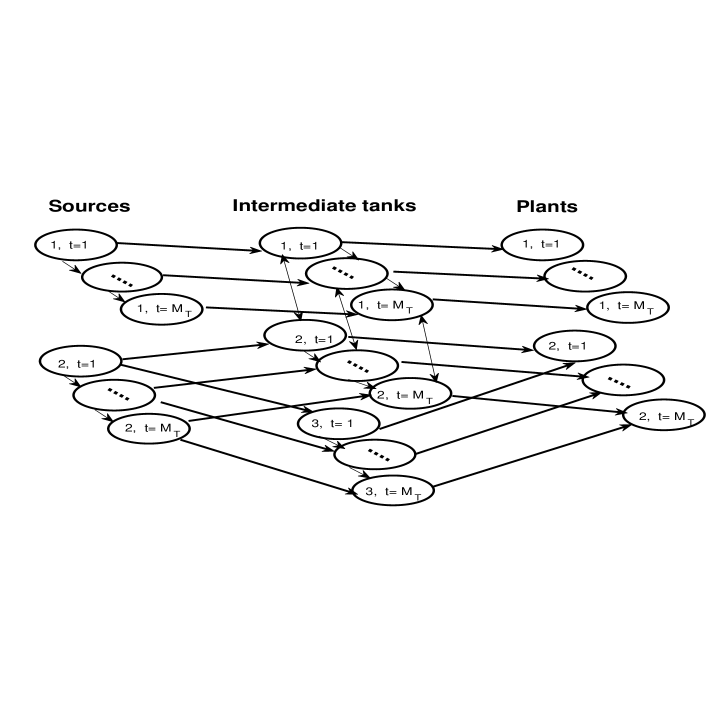
Figure 2: The pooling problem with time discretization

The pooling problem has been represented with various formulations. We formulate P-formulation with time discretization as a nonconvex mixed-integer QCQP. As shown in Figure 2, the pooling problem with time discretization can be viewed as a network with the arcs connecting sources, intermediate tanks, and plants at the same time step.

The objective function of the pooling problem can be modeled as follows:

$$\displaystyle\min_{a,p,q,v}\displaystyle\sum_{t\in T}\sum_{(i,j)\in A}CA_{ij}a_{ij}^{t}+\sum_{t\in T}\sum_{i\in V_{P}}CQ_{i}RC_{i}^{t}v_{i}^{t}.$$

Here $CA_{ij}$ is the transportation cost for the pipeline $(i,j)$, $CQ_{i}$ the penalty cost for the shortage at the $i$th node, and $RC_{i}^{t}$ the required quantity at the $i$th node. The first and second terms of the objective function represent the transportation cost and the penalty cost.

Table 1: The sets, constants and variables of P formulation

Sets
$V_{S}$	the set of sources	$V_{I}$	the set of intermediate tanks
$V_{P}$	the set of plants	$(i,j)$	the pipeline between $i$ and $j$
$I(i)$	the set of entering nodes to the $i$th nodes
$E(i)$	the set of leaving nodes from the $i$th nodes
Constants
$M_{S}$	the number of sources	$M_{I}$	the number of intermediate tanks
$M_{P}$	the number of plants	$M_{T}$	the number of time discretization
$p^{\min}_{i}$	the minimum quantity	$p^{\max}_{i}$	the maximum quantity
$SA^{t}_{i}$	the supply quantity	$SQ^{t}_{i}$	the supply quality
$U_{ij}$	the maximum flow	$L_{ij}$	the minimun flow
$RC^{t}_{i}$	the required quantity	$RQ^{t}_{i}$	the required quality
$CA_{ij}$	the transportation cost for $(i,j)$	$CQ_{i}$	the penalty cost
Variables for the $i$th node at time $t$
$a_{ij}^{t}$	flow in the pipeline $(i,j)$	$p_{i}^{t}$	the quantity
$q_{i}^{t}$	the quality	$u_{ij}^{t}$	binary variables
$v_{i}^{t}$	the quality shortage

For constraints, $v_{i}^{t}$ is introduced to denote the shortage in quality at the $i$th node. If $RQ_{i}^{t}$ is used to denote the required quality at the $i$th node, then

$$v_{i}^{t}=\max\{0,RQ_{i}^{t}-q_{i}^{t}\}\ \ \ (i\in V_{P}\ ,\ t\in T).$$

At each time $t$, each node can be connected to at most one pipeline, therefore we must have

$$u_{ij}^{t}\in\{0,1\},\ \ \sum_{j\in I(i)}u_{ji}^{t}+\sum_{k\in E(i)}u_{ik}^{t}\leq 1\ \ (i\in V,\ (i,j)\in A,\ t\in T=\{1,\dots,M_{T}\}).$$

The flow of each pipeline has a lower and upper bound,

$$u_{ij}^{t}L_{ij}\leq a_{ij}^{t}\leq u_{ij}^{t}U_{ij}\ ((i,j)\in A,t\in T),$$

where $L_{ij}$ and $U_{ij}$ are the lower bound and upper bound for the flow in the pipeline $(i,j)$.

Two constraints can be derived from mixing two kinds of oil with different quantity $p_{i}^{t}$ and quality $q_{i}^{t}$. For instance, we consider mixing oil $1$ and $2$ to produce new oil $3$ in Figure 3. Assume that each node has the quantity, $p_{1},p_{2}$ and $p_{3}$ and the quality, $q_{1},q_{2}$ and $q_{3}$.

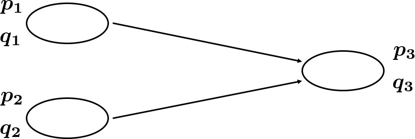
Figure 3: Flow of mixing oil

The constraint for the amount of new oil $p_{3}$ is that it should be equivalent to the sum of oil 1 and 2, i.e., $p_{3}=p_{1}+p_{2}$. Second, the quality of new oil $q_{3}$ should be computed by the weighted average of oil 1 and 2, i.e., $p_{3}q_{3}=p_{1}q_{1}+p_{2}q_{2}$ holds. Thus, necessary constraints for the pooling problem are

$$p^{t+1}_{i}=p_{i}^{t}+SA_{i}^{t}-\sum_{k\in E(i)}a_{ik}^{t},\ \ p_{i}^{t}\geq 0,\ \ p_{i}^{M_{T}+1}=0\ \ \ \ (i\in V_{S},t\in T),$$

$$p^{t+1}_{i}q_{i}^{t+1}=p_{i}^{t}q_{i}^{t}+SA_{i}^{t}SQ_{i}^{t}-\sum_{k\in E(i)}a_{ik}^{t}q_{i}^{t}\ \ \ (i\in V_{S},t\in T),$$

$$p^{t+1}_{i}=p_{i}^{t}+\sum_{k\in I(i)}a_{ki}^{t}-\sum_{k\in E(i)}a_{ik}^{t},\ \ p_{i}^{\min}\leq p_{i}^{t}\leq p_{i}^{\max}\ \ \ (i\in V_{I},t\in T),$$

$$p^{t+1}_{i}q_{i}^{t+1}=p_{i}^{t}q_{i}^{t}+\sum_{k\in I(i)}a_{ki}^{t}q_{k}^{t}-\sum_{k\in E(i)}a_{ik}^{t}q_{i}^{t}\ \ \ (i\in V_{I},t\in T),$$

$$q_{i}^{t}=\frac{1}{RC_{i}^{t}}\sum_{j\in I(i)}a_{ji}^{t}q_{j}^{t}\ \ \ (i\in V_{P},t\in T).$$

Here, $SA_{i}^{t}$ and $SQ_{i}^{t}$ are the supplied quantity and quality at the source $i\in V_{S}$. The constraint $p_{i}^{M_{T}+1}=0$ for $i\in V_{S}$ requires the quantity at the sources should be empty at time $M_{T+1}$.

We describe the formulation of the pooling problem in [16] as follows:

$$(PP) \displaystyle\min_{a,p,q,u,v} \displaystyle\sum_{t\in T}\sum_{(i,j)\in A}CA_{ij}a_{ij}^{t}+\sum_{t\in T}\sum_{i\in V_{P}}CQ_{i}RC_{i}^{t}v_{i}^{t}$$

subject to $$u_{ij}^{t}L_{ij}\leq a_{ij}^{t}\leq u_{ij}^{t}U_{ij}\ \ ((i,j)\in A,t\in T),$$

$$u_{ij}^{t}\in\{0,1\},\ \ \sum_{j\in I(i)}u_{ji}^{t}+\sum_{k\in E(i)}u_{ik}^{t}\leq 1\ \ (i\in V,\ (i,j)\in A,\ t\in T),$$

$$p^{t+1}_{i}=p_{i}^{t}+SA_{i}^{t}-\sum_{k\in E(i)}a_{ik}^{t},\ \ p_{i}^{t}\geq 0\ ,\ p^{M_{T}+1}=0\ \ \ (i\in V_{S},t\in T),$$

$$p^{t+1}_{i}q_{i}^{t+1}=p_{i}^{t}q_{i}^{t}+SA_{i}^{t}SQ_{i}^{t}-\sum_{k\in E(i)}a_{ik}^{t}q_{i}^{t}\ \ (i\in V_{S},t\in T),$$

$$p^{t+1}_{i}=p_{i}^{t}+\sum_{k\in I(i)}a_{ki}^{t}-\sum_{k\in E(i)}a_{ik}^{t},\ \ p_{i}^{\min}\leq p_{i}^{t}\leq p_{i}^{\max}\ \ (i\in V_{I},t\in T),$$

$$p^{t+1}_{i}q_{i}^{t+1}=p_{i}^{t}q_{i}^{t}+\sum_{k\in I(i)}a_{ki}^{t}q_{k}^{t}-\sum_{k\in E(i)}a_{ik}^{t}q_{i}^{t}\ \ \ (i\in V_{I},t\in T),$$

$$q_{i}^{t}=\frac{1}{RC_{i}^{t}}\sum_{j\in I(i)}a_{ji}^{t}q_{j}^{t}\ \ (i\in V_{P},t\in T),$$

$$v_{i}^{t}\geq\max\{0,RQ_{i}^{t}-q_{i}^{t}\}\ \ (i\in V_{P},t\in T).$$

Note that some of the above constraints are quadratic and nonconvex. With nonconvex constraints and the binary variables $u_{ij}^{t}\in\{0,1\}$, the formulation (PP) of the pooling problem is a nonconvex mixed-integer nonlinear programming problem. Each quadratic term of the formulation of the pooling problem is always bilinear, and no squared terms of variables appear in the constraints. Even if $u$ can be removed, the problem is nonconvex, as a result, it is difficult to apply an existing mixed-integer nonlinear programming method. It is known that global optimum solutions cannot be obtained within reasonable time, since the pooling problem has been shown to be NP-hard [5].

Eliminating binary variables

In [16], the pipeline constraints were modified to remove the binary variables $u$ before applying the SDP relaxation problem. We briefly describe the elimination of the binary variables. The constraints involving the binary variables were rewritten with $a^{t}_{ij}$ using the relation between $u^{t}_{ij}$ and $a^{t}_{ij}$. More precisely, the constraints given by

$$\sum_{j\in I(i)}u_{ji}^{t}+\sum_{k\in E(i)}u_{ik}^{t}\leq 1\ \ (i\in V,\ \ t\in T),\ Ê\ u_{ij}^{t}\in\{0,1\}\ \ ((i,j)\in A,\ \ t\in T).$$

require that at most one pipeline for all $i\in V$ and $t\in T$ should be used. Thus, an equivalent constraint can be described in terms of $a$ as follows:

$$\sum_{j,k\in I(i),j\not=k}a_{ji}^{t}a_{ki}^{t}+\sum_{j,k\in E(i),j\not=k}a_{ij}^{t}a_{ik}^{t}+\sum_{j\in I(i),k\in E(i)}a_{ji}^{t}a_{ik}^{t}=0\ \ (i\in V,\ \ t\in T).$$

To remove the binary variables from $u_{ij}^{t}L_{ij}\leq a_{ij}^{t}\leq u_{ij}^{t}U_{ij}\ ((i,j)\in A,\ \ t\in T)$, the lower bound on $a^{t}_{ij}$ was modified to the following nonnegativity,

$$0\leq a^{t}_{ij}\leq U_{ij}\ \ ((i,j)\in A,\ \ t\in T).$$ (2)

As a result, the following problem is derived:

$$\displaystyle\min_{a,p,q,v} \displaystyle\sum_{t\in T}\sum_{(i,j)\in A}CA_{ij}a_{ij}^{t}+\sum_{t\in T}\sum_{i\in V_{P}}CQ_{i}RC_{i}^{t}v_{i}^{t}$$ (3)

subject to $$\sum_{j,k\in I(i),j\not=k}a_{ji}^{t}a_{ki}^{t}+\sum_{j,k\in E(i),j\not=k}a_{ij}^{t}a_{ik}^{t}+\sum_{j,k\in I(i),j\not=k}a_{ji}^{t}a_{ki}^{t}=0\ \ (i\in V,\ \ t\in T),$$

$$0\leq a_{ij}^{t}\leq U_{ij},\ \ \ ((i,j)\in A,\ \ t\in T)$$

$$p^{t+1}_{i}=p_{i}^{t}+SA_{i}^{t}-\sum_{k\in E(i)}a_{ik}^{t}\ ,\ p_{i}^{t}\geq 0\ ,\ p^{M_{T}+1}=0\ \ \ \ (i\in V_{S},t\in T),$$

$$p^{t+1}_{i}q_{i}^{t+1}=p_{i}^{t}q_{i}^{t}+SA_{i}^{t}SQ_{i}^{t}-\sum_{k\in E(i)}a_{ik}^{t}q_{i}^{t}\ \ \ (i\in V_{S},t\in T),$$

$$p^{t+1}_{i}=p_{i}^{t}+\sum_{k\in I(i)}a_{ki}^{t}-\sum_{k\in E(i)}a_{ik}^{t}\ \ \ p_{i}^{\min}\leq p_{i}^{t}\leq p_{i}^{\max}\ \ \ (i\in V_{I},t\in T),$$

$$p^{t+1}_{i}q_{i}^{t+1}=p_{i}^{t}q_{i}^{t}+\sum_{k\in I(i)}a_{ki}^{t}q_{k}^{t},-\sum_{k\in E(i)}a_{ik}^{t}q_{i}^{t}\ \ \ (i\in V_{I},t\in T),$$

$$q_{i}^{t}=\frac{1}{RC_{i}^{t}}\sum_{j\in I(i)}a_{ji}^{t}q_{j}^{t}\ \ \ (i\in V_{P},t\in T),$$

$$v_{i}^{t}\geq\max\{0,RQ_{i}^{t}-q_{i}^{t}\}\ \ \ (i\in V_{P},t\in T).$$

While the number of constraints in (3) is the same as the number of constraints of the original pooling problem, the number of variables in (3) is small compared to the original pooling problem. Thus, (3) can be solved more efficiently by conic relaxation methods than the original pooling problem.

2.3 The proposed formulation

Although the modified problem (3) in [16] has reduced the number of variables and no binary variables, (3) may not have an interior point. If SDP relaxations are used to solve problems with no interior point, as in [16], SDP solvers based on primal-dual interior-pont methods [17, 18, 20, 21] frequently fail due to numerical instability. To avoid such numerical difficulty, we relax the equality to inequalities. For instance, we first transform equality constraints of the form $a^{T}x=b$ into $-\lambda\leq a^{T}x-b\leq\lambda$ introducing by a new variable $\lambda$. Then, we add $\lambda$ to the objective function as a penalty function.

Our formulation of the pooling problem is:

(4)

$$\displaystyle\min_{a,p,q,v} \displaystyle\sum_{t\in T}\sum_{(i,j)\in A}CA_{ij}a_{ij}^{t}+\sum_{t\in T}\sum_{i\in V_{P}}CQ_{i}RC_{i}^{t}v_{i}^{t}+\delta\sum_{t\in T}\sum_{(i,j)\in A}\lambda_{i}^{t}$$

subject to $$-\lambda_{i}^{t}\leq\sum_{j,k\in I(i),j\not=k}a_{ji}^{t}a_{ki}^{t}+\sum_{j,k\in E(i),j\not=k}a_{ij}^{t}a_{ik}^{t}+\sum_{j,k\in I(i),j\not=k}a_{ji}^{t}a_{ki}^{t}\leq\lambda_{i}^{t}\ \ (i\in V,\ \ t\in T),$$

$$0\leq a_{ij}^{t}\leq U_{ij}\ \ \ ((i,j)\in A,\ \ t\in T),$$

$$-\lambda_{i}^{t}\leq-p^{t+1}_{i}+p_{i}^{t}+SA_{i}^{t}-\sum_{k\in E(i)}a_{ik}^{t}\leq\lambda_{i}^{t},\ \ p_{i}^{t}\geq 0,\ \ p^{M_{T}+1}=0\ \ \ \ (i\in V_{S},t\in T),$$

$$-\lambda_{i}^{t}\leq-p^{t+1}_{i}q_{i}^{t+1}+p_{i}^{t}q_{i}^{t}+SA_{i}^{t}SQ_{i}^{t}-\sum_{k\in E(i)}a_{ik}^{t}q_{i}^{t}\leq\lambda_{i}^{t}\ \ \ (i\in V_{S},\ t\in T),$$

$$-\lambda_{i}^{t}\leq-p^{t+1}_{i}+p_{i}^{t}+\sum_{k\in I(i)}a_{ki}^{t}-\sum_{k\in E(i)}a_{ik}^{t}\leq\lambda_{i}^{t},\ \ \ p_{i}^{\min}\leq p_{i}^{t}\leq p_{i}^{\max}\ \ \ (i\in V_{I},\ t\in T),$$

$$-\lambda_{i}^{t}\leq-p^{t+1}_{i}q_{i}^{t+1}+p_{i}^{t}q_{i}^{t}+\sum_{k\in I(i)}a_{ki}^{t}q_{k}^{t}-\sum_{k\in E(i)}a_{ik}^{t}q_{i}^{t}\leq\lambda_{i}^{t}\ \ \ (i\in V_{I},\ t\in T),$$

$$-\lambda_{i}^{t}\leq-q_{i}^{t}+\frac{1}{RC_{i}^{t}}\sum_{j\in I(i)}a_{ji}^{t}q_{j}^{t}\leq\lambda_{i}^{t}\ \ \ (i\in V_{P},\ t\in T),$$

$$v_{i}^{t}\geq\max\{0,RQ_{i}^{t}-q_{i}^{t}\}\ \ \ (i\in V_{P},\ t\in T),\ \ \lambda_{i}^{t}\geq 0\ (i\in V,\ t\in T),$$

where $\delta$ is a penalty parameter.

For the subsequent discussion, we express (4) using variable $x$ defined as $\mbox{\boldmath$x$}=\{\mbox{\boldmath$a$},\mbox{\boldmath$p$},\mbox{\boldmath$q$},\mbox{\boldmath$v$}\}$. More precisely, each set of variables are ordered in the following order.

$$a =\{a^{1},\dots,a^{M_{T}}\},\ \$$

$$\mbox{\boldmath$a$}^{t} =\{a^{t}_{ij}\|(i,j)\in A\}\ \ (t\in T),$$

$$p =\{p^{2},\dots,p^{M_{T}},p^{M_{T}+1}\},\ \$$

$$\mbox{\boldmath$p$}^{t} =\{p^{t}_{i},\ p^{t}_{j}\|i\in V_{S},\ j\in V_{I}\}\ \ (t\in T\ \backslash\{1\}),\ \$$

$$\mbox{\boldmath$p$}^{M_{T}+1} =\{p^{M_{T}+1}_{i}\|i\in V_{I}\},\ \$$

$$q =\{q^{1},\dots,q^{M_{T}+1}\},\ \$$

$$\mbox{\boldmath$q$}^{1} =\{q^{1}_{i}\|i\in V_{P}\},\ \ \ \$$

$$\mbox{\boldmath$q$}^{t} =\{q^{t}_{i},\ q^{t}_{j},\ q^{t}_{k}\|i\in V_{S},\ j\in V_{I},\ k\in V_{P}\}\ \ (t\in T\ \backslash\{1\}),\ \$$

$$\mbox{\boldmath$q$}^{M_{T}+1} =\{q^{M_{T}+1}_{i}\|i\in V_{I}\},\ \$$

$$v =\{v^{1},\dots,v^{M_{T}}\},\ \$$

$$\mbox{\boldmath$v$}^{t} =\{v^{t}_{i}\|i\in V_{P}\}\ \ (t\in T).$$

Let $n$ be the length of $x$, that is, $\mbox{\boldmath$x$}\in\mbox{$\mathbb{R}$}^{n}_{+}$ where $\mbox{$\mathbb{R}$}^{n}_{+}$ denotes the space of $n$-dimensional column vectors of nonnegative numbers. We also let $\mbox{$\mathbb{R}$}^{n}$ be the space of $n$-dimensional column vectors $\mbox{$\mathbb{R}$}^{d\times n}$ the space of $d\times n$ real matrices, and $\mbox{$\mathbb{S}$}^{n}$ the space of $n\times n$ symmetric matrices.

Let the number of the quadratic equalities of (4) is $m$, the number of linear equality constraints $d$, the number of linear inequalities $e$. Then, with appropriately chosen matrices $\mbox{\boldmath$Q$}_{k}\in\mbox{$\mathbb{S}$}^{n}\ (k=1,\ldots,m),\ \mbox{\boldmath$L$}_{m+1}\in\mbox{$\mathbb{R}$}^{d\times n},\mbox{\boldmath$L$}_{m+2}\in\mbox{$\mathbb{R}$}^{e\times n},$ and $\mbox{\boldmath$q$}_{0}\in\mbox{$\mathbb{R}$}^{n}$, we assume that (3) can be written in the following general form:

$$\displaystyle\min_{\mbox{\boldmath$x$}\in\mathbb{R}^{n}} \mbox{\boldmath$q$}_{0}^{T}\mbox{\boldmath$x$}$$

subject to $$\mbox{\boldmath$x$}^{T}\mbox{\boldmath$Q$}_{k}\mbox{\boldmath$x$}+\mbox{\boldmath$q$}_{k}^{T}\mbox{\boldmath$x$}+\gamma_{k}=0\ \ \ (k=1,\dots,m),\ \$$

$$\ \mbox{\boldmath$L$}_{m+1}\mbox{\boldmath$x$}=\mbox{\boldmath$b$}_{m+1},\ \ \mbox{\boldmath$L$}_{m+2}\mbox{\boldmath$x$}\leq\mbox{\boldmath$b$}_{m+2},$$

$$\mbox{\boldmath$\ell$}\leq\mbox{\boldmath$x$}\leq\mbox{\boldmath$u$},\$$

where $\mbox{\boldmath$\ell$},\mbox{\boldmath$u$}\in\mbox{$\mathbb{R}$}^{n}$ mean, respectively, the lower and upper bounds for $x$, and $\mbox{\boldmath$b$}_{m+1}\in\mbox{$\mathbb{R}$}^{d},\mbox{\boldmath$b$}_{m+2}\in\mbox{$\mathbb{R}$}^{e}$.

Consequently, (4) can be expressed as the following general form:

$$\displaystyle\min_{\mbox{\boldmath$x$}\in\mathbb{R}^{n},\ \lambda\in\mathbb{R}^{m+d}} \mbox{\boldmath$q$}_{0}^{T}\mbox{\boldmath$x$}+\delta\sum_{i=1}^{m+d}\lambda_{i}$$ (5)

subject to $$-\lambda^{1}_{k}\leq\mbox{\boldmath$x$}^{T}\mbox{\boldmath$Q$}_{k}\mbox{\boldmath$x$}+\mbox{\boldmath$q$}_{k}^{T}\mbox{\boldmath$x$}+\gamma_{k}\leq\lambda^{1}_{k}\ \ \ (k=1,\dots,m),\ \$$

$$-\mbox{\boldmath$\lambda$}^{2}_{m+1}\leq\mbox{\boldmath$L$}_{m+1}\mbox{\boldmath$x$}-\mbox{\boldmath$b$}_{m+1}\leq\mbox{\boldmath$\lambda$}^{2}_{m+1},\ \ \mbox{\boldmath$L$}_{m+2}\mbox{\boldmath$x$}\leq\mbox{\boldmath$b$}_{m+2},\ \$$

$$\mbox{\boldmath$\lambda$}\geq 0\ ,\ \mbox{\boldmath$\ell$}\leq\mbox{\boldmath$x$}\leq\mbox{\boldmath$u$},$$

where $\mbox{\boldmath$\lambda$}=[\mbox{\boldmath$\lambda$}^{1},\mbox{\boldmath$\lambda$}^{2}_{m+1}]^{T}\in\mbox{$\mathbb{R}$}^{m+d}$ and $\mbox{\boldmath$\lambda$}^{2}_{m+1}\in\mbox{$\mathbb{R}$}^{d}$.

If we let $\mbox{\boldmath$q$}_{m+r}$ be the $r$th row of $\mbox{\boldmath$L$}_{m+1}\ (r=1,\ldots,d)$ and $\mbox{\boldmath$q$}_{m+d+\rho}$ be the $\rho$th row of $\mbox{\boldmath$L$}_{m+2}\ (\rho=1,\ldots,e)$, then (5) is written as follows:

$$\displaystyle\min_{\mbox{\boldmath$x$}\in\mathbb{R}^{n},\ \mbox{\boldmath$\lambda$}\in\mathbb{R}^{m+d}} \mbox{\boldmath$q$}_{0}^{T}\mbox{\boldmath$x$}+\delta\sum_{i=1}^{m+d}\lambda_{i}$$ (6)

subject to $$\mbox{\boldmath$x$}^{T}\mbox{\boldmath$Q$}_{k}\mbox{\boldmath$x$}+\mbox{\boldmath$q$}_{k}^{T}\mbox{\boldmath$x$}-\lambda^{1}_{k}+\gamma_{k}\leq 0,$$

$$-\mbox{\boldmath$x$}^{T}\mbox{\boldmath$Q$}_{k}\mbox{\boldmath$x$}-\mbox{\boldmath$q$}_{k}^{T}\mbox{\boldmath$x$}-\lambda^{1}_{k}-\gamma_{k}\leq 0\ (k=1,\dots,m),\ \$$

$$\mbox{\boldmath$q$}_{m+r}\mbox{\boldmath$x$}-(\mbox{\boldmath$\lambda$}^{2}_{m+1})_{r}-(\mbox{\boldmath$b$}_{m+1})_{r}\leq 0,$$

$$-\mbox{\boldmath$q$}_{m+r}\mbox{\boldmath$x$}-(\mbox{\boldmath$\lambda$}^{2}_{m+1})_{r}+(\mbox{\boldmath$b$}_{m+1})_{r}\leq 0\ (r=1,\ldots,d),$$

$$\mbox{\boldmath$q$}_{m+r+\rho}\mbox{\boldmath$x$}-(\mbox{\boldmath$b$}_{m+2})_{\rho}\leq 0\ (\rho=1,\ldots,e),\$$

$$\mbox{\boldmath$\lambda$}\geq 0\ ,\ \mbox{\boldmath$\ell$}\leq\mbox{\boldmath$x$}\leq\mbox{\boldmath$u$}.$$

Notice that all the diagonal elements of $\mbox{\boldmath$Q$}_{1},\ldots,\mbox{\boldmath$Q$}_{m}$ in the quadratic constraints of (6) are zeros. This will be exploited in Section 4.

3 SDP, SOCP and LP relaxations

We give a brief description of an SDP relaxation of general QCQPs which include (4). Then, SOCP [13] and LP relaxations of general QCQPs are described using the scaled diagonally dominant (SDD) matrices and diagonally dominant (DD) matrices, respectively.

3.1 SDP relaxations

Let $\mbox{\boldmath$w$}\in\mbox{$\mathbb{R}$}^{n}$. Consider a general form of QCQP:

$$\begin{array}[]{rcl}\zeta^{*}:=\min&&\mbox{\boldmath$w$}^{T}\mbox{\boldmath$Q$}_{0}\mbox{\boldmath$w$}+\mbox{\boldmath$\beta$}_{0}^{T}\mbox{\boldmath$w$}+\gamma_{0}\\ \mbox{subject to}&&\mbox{\boldmath$w$}^{T}\mbox{\boldmath$Q$}_{k}\mbox{\boldmath$w$}+\mbox{\boldmath$\beta$}_{k}^{T}\mbox{\boldmath$w$}+\gamma_{k}\leq 0\quad(k=1,\ldots,m),\end{array}$$ (9)

where $\mbox{\boldmath$Q$}_{k}\in\mbox{$\mathbb{S}$}^{n},\ \mbox{\boldmath$\beta$}_{k}\in\mbox{$\mathbb{R}$}^{n}\ (k=0,\ldots,m)$ and $\gamma_{k}\in\mbox{$\mathbb{R}$}\ (k=1,\ldots,m)$. Since $\mbox{\boldmath$Q$}_{k}\in\mbox{$\mathbb{S}$}^{n}\ (k=0,\ldots,m)$ is not necessarily positive semidefinite, (9) is a nonconvex problem.

Introducing a new variable matrix $\mbox{\boldmath$W$}\in\mbox{$\mathbb{S}$}^{n}$, we let

$$\bar{\mbox{\boldmath$Q$}}_{k}:=\left(\begin{array}[]{cc}\gamma_{k}&\mbox{\boldmath$\beta$}_{k}^{T}/2\\ \mbox{\boldmath$\beta$}_{k}/2&\mbox{\boldmath$Q$}_{k}\end{array}\right),\ \bar{\mbox{\boldmath$W$}}:=\left(\begin{array}[]{cc}w_{00}&\mbox{\boldmath$w$}^{T}\\ \mbox{\boldmath$w$}&\mbox{\boldmath$W$}\end{array}\right),\mbox{ and }\bar{\mbox{\boldmath$H$}}_{0}:=\left(\begin{array}[]{cc}1&\mbox{\bf 0}^{T}\\ \mbox{\bf 0}&\mbox{\boldmath$O$}\end{array}\right).$$

Then, an SDP relaxation of (9) is given by

$$\begin{array}[]{rcl}\zeta_{SDP}^{*}:=\min&&\bar{\mbox{\boldmath$Q$}}_{0}\bullet\bar{\mbox{\boldmath$W$}}\\ \mbox{subject to}&&\bar{\mbox{\boldmath$Q$}}_{k}\bullet\bar{\mbox{\boldmath$W$}}\leq 0\quad(k=1,\ldots,m),\\ &&\bar{\mbox{\boldmath$H$}}_{0}\bullet\bar{\mbox{\boldmath$W$}}=1,\\ &&\bar{\mbox{\boldmath$W$}}\in\mbox{$\mathbb{S}$}_{+}^{n+1},\end{array}$$ (14)

where the inner product $\bar{\mbox{\boldmath$Q$}}\bullet\bar{\mbox{\boldmath$W$}}$ means the standard inner product between two symmetric matrices, i.e., $\bar{\mbox{\boldmath$Q$}}\bullet\bar{\mbox{\boldmath$W$}}=\sum_{i}\sum_{k}\bar{Q}_{ik}\bar{W}_{ik}$.

3.2 SOCP relaxations

In [13], an SOCP relaxation was proposed using the $2\times 2$ principle submatrices of the variable matrix $\bar{\mbox{\boldmath$W$}}$ of (14). They showed that the SOCP relaxation provides the exact optimal solution for QCQP if the off-diagonal elements of $\bar{\mbox{\boldmath$Q$}}_{k}$ $(k=0,\ldots,m)$ are nopositive. The SOCP relaxation in [13] is closely related to the dual of the first level relaxation of the hierarchy of the scaled diagonally dominant sum-of-squares (SDSOS) relaxations proposed in [3]. By applying the approach in [13], we obtain the following SOCP relaxation:

$$\left.\begin{array}[]{llll}\mbox{min }&\bar{\mbox{\boldmath$Q$}}_{0}\bullet\bar{\mbox{\boldmath$W$}}\\ \mbox{subject to }&\bar{\mbox{\boldmath$Q$}}_{k}\bullet\bar{\mbox{\boldmath$W$}}\leq 0\ (1\leq k\leq m),\ \bar{\mbox{\boldmath$H$}}_{0}\bullet\bar{\mbox{\boldmath$W$}}=1,\\ &\bar{W}_{jj}\geq 0\ (1\leq j\leq n+1),\\ &(\bar{W}_{ij})^{2}\leq\bar{W}_{ii}\bar{W}_{jj}\ (1\leq i<j\leq n+1).\end{array}\right\}$$ (15)

Using

$$w^{2}\leq\xi\eta,\ \xi\geq 0\ \mbox{ and }\eta\geq 0\mbox{ if and only if }\left\|\left(\begin{array}[]{c}\xi-\eta\\ 2w\end{array}\right)\right\|\leq\xi+\eta,$$ (16)

(15) is converted to an SOCP. Thus, the following SOCP is equivalent to the problem (15).

$$\left.\begin{array}[]{llll}\zeta_{SOCP}^{*}:=\mbox{min }&\bar{\mbox{\boldmath$Q$}}_{0}\bullet\bar{\mbox{\boldmath$W$}}\\ \mbox{subject to }&\bar{\mbox{\boldmath$Q$}}_{p}\bullet\bar{\mbox{\boldmath$W$}}\leq 0\ (1\leq p\leq m),\ \bar{\mbox{\boldmath$H$}}_{0}\bullet\bar{\mbox{\boldmath$W$}}=1,\\ &\left\|\left(\begin{array}[]{c}\bar{W}_{ii}-\bar{W}_{jj}\\ 2\bar{W}_{ij}\end{array}\right)\right\|\leq\bar{W}_{ii}+\bar{W}_{jj}\ (1\leq i<j\leq n+1).\end{array}\right\}$$ (17)

Since $\bar{\mbox{\boldmath$W$}}\in\mbox{$\mathbb{S}$}^{n}_{+}$ implies $(\bar{W}_{ij})^{2}\leq\bar{W}_{ii}\bar{W}_{jj}\ (1\leq i<j\leq n+1)$, the optimal value $\zeta_{SOCP}^{*}$ of (17) is weaker than $\zeta_{SDP}^{*}$ of (14):

$$\zeta_{SOCP}^{*}\leq\zeta_{SDP}^{*}\leq\zeta^{*}.$$

3.3 LP relaxations

We derive LP relaxations of (9) using the diagonally dominant sum-of-squares relaxation (DSOS) in [3].

Consider the cone of diagonally dominant matrices of dimension $n+1$ defined by

$$\mbox{$\cal D$}^{n+1}:=\left\{\mbox{\boldmath$W$}\in\mbox{$\mathbb{S}$}^{n+1}:W_{ii}\geq\sum_{j\neq i}|W_{ij}|\quad(1\leq i\leq n+1)\right\}.$$

In [8], the dual of $\mbox{$\cal D$}^{n+1}$ is given by

$$(\mbox{$\cal D$}^{n+1})^{*} := \left\{\mbox{\boldmath$W$}\in\mbox{$\mathbb{S}$}^{n+1}:\mbox{\boldmath$w$}^{T}\mbox{\boldmath$W$}\mbox{\boldmath$w$}\geq 0\mbox{ for }\forall\mbox{\boldmath$w$}\mbox{ with at most 2 nonzero elements }1\mbox{ or -1}\right\}$$

$$= \left\{\mbox{\boldmath$W$}\in\mbox{$\mathbb{S}$}^{n+1}:W_{ii}\geq 0\ (1\leq i\leq n+1),\ W_{ii}+W_{jj}-2|W_{ij}|\geq 0\quad(1\leq i<j\leq n+1)\right\}$$

Using $(\mbox{$\cal D$}^{n+1})^{*}$, an LP relaxation of (9) can be derived as

$$\left.\begin{array}[]{llll}\zeta_{LP}^{*}:=\mbox{min }&\bar{\mbox{\boldmath$Q$}}_{0}\bullet\bar{\mbox{\boldmath$W$}}\\ \mbox{subject to }&\bar{\mbox{\boldmath$Q$}}_{k}\bullet\bar{\mbox{\boldmath$W$}}\leq 0\ (1\leq k\leq m),\ \bar{\mbox{\boldmath$H$}}_{0}\bullet\bar{\mbox{\boldmath$W$}}=1,\\ &\bar{W}_{ii}\geq 0\ (1\leq i\leq n+1),\\ &\bar{W}_{ii}+\bar{W}_{jj}-2|\bar{W}_{ij}|\geq 0\quad(1\leq i<j\leq n+1).\end{array}\right\}$$ (18)

Let $\bar{\mbox{\boldmath$W$}}$ be a feasible solution of (17). Then, $|\bar{W}_{ij}|\leq\sqrt{\bar{W}_{ii}\bar{W}_{jj}}\ \ (1\leq i<j\leq n+1).$ Since $\sqrt{\bar{W}_{ii}\bar{W}_{jj}}\leq(\bar{W}_{ii}+\bar{W}_{jj})/2$ always holds for all nonnegative $\bar{W}_{ii}$ and $\bar{W}_{jj}$, $\bar{\mbox{\boldmath$W$}}$ is a feasible solution of (18). Thus, the LP relaxation (18) is an weaker relaxation than the SOCP relaxation (17) and the following relation holds for the optimal values of the three relaxations:

$$\zeta^{*}_{LP}\leq\zeta^{*}_{SOCP}\leq\zeta^{*}_{SDP}\leq\zeta^{*}.$$ (19)

4 The equivalence of the optimal values of SDP, SOCP and LP relaxations

Now, we show the equivalence among the optimal values of (14), (17) and (18) under the following assumptions. As mentioned at the end of Section 2, the pooling problem satisfies the following assumption.

Assumption 4.1.

All the diagonal elements in $\mbox{\boldmath$Q$}_{0},\mbox{\boldmath$Q$}_{1},\ldots,\mbox{\boldmath$Q$}_{m}$ of (9) are zeros.

Theorem 4.1.

Suppose that Assumption 4.1 holds. Then, $\zeta_{SDP}^{*}=\zeta_{SOCP}^{*}=\zeta_{LP}^{*}$.

Proof.

Let $\bar{\mbox{\boldmath$W$}}=\left(\begin{array}[]{cc}w_{00}&\mbox{\boldmath$w$}^{T}\\ \mbox{\boldmath$w$}&\mbox{\boldmath$W$}\end{array}\right)$ be a feasible solution of (18). It always holds that $w_{00}=1$ by the constraint $\bar{\mbox{\boldmath$H$}}_{0}\bullet\bar{\mbox{\boldmath$W$}}=1$. If we add a sufficiently large number $\alpha\geq\lambda_{\max}\left(\frac{\mbox{\boldmath$w$}\mbox{\boldmath$w$}^{T}}{w_{00}}-\mbox{\boldmath$W$}\right)$ to the diagonal of $\bar{\mbox{\boldmath$W$}}$ except the first diagonal element $w_{00}$ of $\bar{\mbox{\boldmath$W$}}$, the resulting matrix $\left(\begin{array}[]{cc}w_{00}&\mbox{\boldmath$w$}^{T}\\ \mbox{\boldmath$w$}&\mbox{\boldmath$W$}+\alpha\mbox{\boldmath$I$}\end{array}\right)$ becomes positive semidefinite by the Schur complement. Here $\lambda_{\max}$ means the largest eigenvalue. The inequality constraints, however, still hold and the objective value remains same, since the diagonal elements in $\mbox{\boldmath$Q$}_{0},\ldots,\mbox{\boldmath$Q$}_{m}$ are zeros by Assumption 4.1. Thus, $\left(\begin{array}[]{cc}w_{00}&\mbox{\boldmath$w$}^{T}\\ \mbox{\boldmath$w$}&\mbox{\boldmath$W$}+\alpha\mbox{\boldmath$I$}\end{array}\right)$ is a feasible solution of the SDP relaxation (14). Therefore, we can construct a feasible solution in the SDP relaxation whose objective value is same as $\bar{\mbox{\boldmath$W$}}$, and this leads to $\zeta_{SDP}^{*}\leq\zeta_{LP}^{*}$. In view of this with (19), the desired result $\zeta_{SDP}^{*}=\zeta_{SOCP}^{*}=\zeta_{LP}^{*}$ follows. ∎

From Theorem 4.1, we show the relationship among the optimal values of the primal and dual problems in the subsequent discussion. The dual of (14) can be written as

$$\begin{array}[]{rcl}\mu_{SDP}^{*}:=\max&&\mu\\ \mbox{subject to}&&\bar{\mbox{\boldmath$Q$}}_{0}+\sum_{k=1}^{m}\eta_{k}\bar{\mbox{\boldmath$Q$}}_{k}-\mu\bar{\mbox{\boldmath$H$}}_{0}-\bar{\mbox{\boldmath$S$}}=\mbox{\boldmath$O$},\\ &&\eta_{1},\ldots,\eta_{m}\geq 0,\ \mu\in\mbox{$\mathbb{R}$},\\ &&\bar{\mbox{\boldmath$S$}}\in\mbox{$\mathbb{S}$}_{+}^{n+1}.\end{array}$$ (24)

By Assumption 4.1, this problem has no interior point. Thus, the positive duality gap between $\zeta_{SDP}^{*}$ and $\mu_{SDP}^{*}$ might exist as the Slater condition does not hold. In the following Corollary 4.1, we show that there is no duality gap, that is, $\zeta_{SDP}^{*}=\mu_{SDP}^{*}$, using the dual of the SOCP relaxation (17) and the LP relaxation (18). These dual problems are closely related to scaled diagonally dominant sum of squares (SDSOS) and diagonally dominant sum of squares (DSOS) in [3].

In [2], SDSOS relaxations were proposed using SDD matrices. A matrix $\mbox{\boldmath$B$}\in\mbox{$\mathbb{S}$}^{n}$ is SDD if and only if it can be expressed as

$$\mbox{\boldmath$B$}=\sum_{i=1}^{n-1}\sum_{j=i+1}^{n}\mbox{\boldmath$B$}^{ij},$$

where the nonzero elements of $\mbox{\boldmath$B$}^{ij}\in\mbox{$\mathbb{S}$}^{n}$ are from the $2\times 2$ principal submatrix of a positive semidefinite matrix $\mbox{\boldmath$C$}\in\mbox{\boldmath$S$}^{n}_{+}$ with $i$th and $j$th rows and columns of $C$ and all the other elements of $\mbox{\boldmath$B$}^{ij}$ are zero. More precisely, $\mbox{\boldmath$B$}^{ij}$ is a symmetric matrix with nonzero elements only in $(i,i)$th, $(i,j)$th, $(j,i)$th and $(j,j)$th positions such that $\left[\begin{array}[]{cc}(\mbox{\boldmath$B$}^{ij})_{ii}&(\mbox{\boldmath$B$}^{ij})_{ij}\\ (\mbox{\boldmath$B$}^{ij})_{ij}&(\mbox{\boldmath$B$}^{ij})_{jj}\end{array}\right]\in\mbox{$\mathbb{S}$}^{2}_{+}$. Thus, each $\mbox{\boldmath$B$}^{ij}\in\mbox{$\mathbb{S}$}^{n}$ is positive semidefinite. Let $\mbox{$\cal S$}\mbox{$\cal D$}^{n}$ be the cone of SDD matrices. It is well-known that any DD matrix is SDD, therefore, $\mbox{$\cal D$}^{n}\subset\mbox{$\cal S$}\mbox{$\cal D$}^{n}\subset\mbox{$\mathbb{S}$}_{+}^{n}$ holds.

Replacing $\bar{\mbox{\boldmath$S$}}\in\mbox{$\mathbb{S}$}_{+}^{n+1}$ in (24) by $\bar{\mbox{\boldmath$S$}}\in\mbox{$\cal S$}\mbox{$\cal D$}^{n+1}$ corresponds to the first level of the hierarchy of SDSOS relaxation for QCQPs in [2], and it is the dual of (17):

$$\begin{array}[]{rcl}\mu_{SOCP}^{*}:=\max&&\mu\\ \mbox{subject to}&&\bar{\mbox{\boldmath$Q$}}_{0}+\sum_{k=1}^{m}\eta_{k}\bar{\mbox{\boldmath$Q$}}_{k}-\mu\bar{\mbox{\boldmath$H$}}_{0}-\bar{\mbox{\boldmath$S$}}=\mbox{\boldmath$O$},\\ &&\eta_{1},\ldots,\eta_{m}\geq 0,\ \mu\in\mbox{$\mathbb{R}$},\\ &&\bar{\mbox{\boldmath$S$}}\in\mbox{$\cal S$}\mbox{$\cal D$}^{n+1}.\end{array}$$ (29)

The dual of (18) is given as

$$\begin{array}[]{rcl}\mu_{LP}^{*}:=\max&&\mu\\ \mbox{subject to}&&\bar{\mbox{\boldmath$Q$}}_{0}+\sum_{k=1}^{m}\eta_{k}\bar{\mbox{\boldmath$Q$}}_{k}-\mu\bar{\mbox{\boldmath$H$}}_{0}-\bar{\mbox{\boldmath$S$}}=\mbox{\boldmath$O$},\\ &&\eta_{1},\ldots,\eta_{m}\geq 0,\ \mu\in\mbox{$\mathbb{R}$},\\ &&\bar{\mbox{\boldmath$S$}}\in\mbox{$\cal D$}^{n+1}.\end{array}$$ (34)

In general,

$$\mu_{SDP}^{*}\geq\mu_{SOCP}^{*}\geq\mu_{LP}^{*}$$ (35)

holds from $\mbox{$\cal D$}^{n+1}\subset\mbox{$\cal S$}\mbox{$\cal D$}^{n+1}\subset\mbox{$\mathbb{S}$}_{+}^{n+1}$.

We will show that the primal problems and the dual problems attain the same optimal values, and this indicates that there is no duality gap between the SDP relaxation (14) and (24).

Corollary 4.1.

Under Assumption 4.1, it holds that

$$\zeta^{*}_{SDP}=\zeta^{*}_{SOCP}=\zeta^{*}_{LP}=\mu_{LP}^{*}=\mu_{SOCP}^{*}=\mu_{SDP}^{*}.$$

Proof.

For (24), we let $\bar{\mbox{\boldmath$S$}}=\left(\begin{array}[]{cc}s_{00}&\mbox{\boldmath$s$}^{T}\\ \mbox{\boldmath$s$}&\mbox{\boldmath$S$}\end{array}\right)$. From Assumption 4.1, the diagonal of $S$ is zero. Since $\mbox{\boldmath$S$}\in\mbox{$\mathbb{S}$}^{n}_{+}$, we have $\mbox{\boldmath$S$}=\mbox{\boldmath$O$}$, thus, $\bar{\mbox{\boldmath$S$}}\in\mbox{$\mathbb{S}$}^{n+1}_{+}$ leads to $\mbox{\boldmath$s$}=\mbox{\bf 0}$. Hence, $\eqref{SDPD}$ is equivalent to the following problem:

$$\begin{array}[]{rcl}\max&&\mu\\ \mbox{subject to}&&\gamma_{0}+\sum_{k=1}^{m}\eta_{k}\gamma_{k}-\mu-s_{00}\geq 0,\\ &&\mbox{\boldmath$q$}_{0}+\sum_{k=1}^{m}\eta_{k}\mbox{\boldmath$q$}_{k}=\mbox{\bf 0},\\ &&\mbox{\boldmath$Q$}_{0}+\sum_{k=1}^{m}\eta_{k}\mbox{\boldmath$Q$}_{k}=\mbox{\boldmath$O$},\\ &&\eta_{1},\ldots,\eta_{m}\geq 0,\ \mu\in\mbox{$\mathbb{R}$},\ s_{00}\geq 0.\end{array}$$ (41)

Similarly, for (34), we can show that $\mbox{\boldmath$S$}=\mbox{\boldmath$O$}$ and $\mbox{\boldmath$s$}=\mbox{\bf 0}$ using the zero diagonal of $\bar{\mbox{\boldmath$S$}}$. As a result, (34) is equivalent to (41), and the optimal values of (34) and (41) coincide, i.e., $\mu_{SDP}^{*}=\mu_{LP}^{*}$. Since the duality theorem holds on linear programming problems regardless of the existence of interior points, the optimal values of (18) and (34) are equivalent, i.e., $\zeta_{LP}^{*}=\mu_{LP}^{*}$. By $\mu_{SDP}^{*}=\mu_{LP}^{*}=\zeta_{LP}^{*}$, (19), (35) and Theorem 4.1, the desired result follows.

∎

5 Computational methods

In this section, we discuss two computational methods for adjusting and refining an approximate solution obtained by the SOCP or LP relaxation of the pooling problem. As the pooling problem is NP-hard, only approximate solutions can be obtained by the relaxation methods. In addition, the bounds for the variables of the pooling problem have been modified when binary variables have been removed in (2). As a result, an approximate solution by SOCP or LP relaxation may not be a solution to the original problem.

In Nishi’s method [16], a mixed-integer linear program was first solved for finding a feasible solution of the original pooling problem. Then, fmincon in Matlab, a nonlinear programming solver, was applied to find a local optimum solution. This step turned out to be very time-consuming. To improve the computational efficiency for finding a solution that satisfies the plant requirements, we propose a rescheduling method based on successive refining the solution obtained by solving the SOCP or LP problem.

Nishi [16]’s method can be described as follows:

Algorithm 5.1: Nishi’s method Step 1. Solve an SDP relaxation of the pooling problem (3). Step 2. Apply a procedure called FFS (finding feasible solution) to find a feasible solution $x$. Step 3. Use a general nonlinear programming solver (fmincon) starting from $x$ for a local optimal solution.

We note that the feasible solution $x$ obtained in Step 2 is not necessarily a local minimum of the original problem. Step 3 is very time-consuming, as shown in numerical results in Section 6.

In our method, the SOCP or LP relaxation is used instead of the SDP relaxation. We also propose a rescheduling method for Step 3 of Nishi’s method. More precisely, after applying applying the SOCP or LP relaxation and FFS, which is described in Section 5.1 in detail, an approximate solution is further refined by the rescheduling method. The main steps of our method is described as follows:

Algorithm 5.2: The proposed method Step 1. Solve the SOCP or LP relaxation (18) of the pooling problem. Step 2. Apply FFS to obtain a feasible solution $x$. Step 3. Perform the proposed rescheduling method.

We briefly review FFS [16] in Section 5.1 and describe our proposed rescheduling method in Section 5.2.

5.1 A method for finding a feasible solution

As a solution attained by the SDP, SOCP or LP relaxation is not necessarily feasible for the original problem, the following mixed-integer linear problem was introduced to find a feasible solution in [16] as the first step of the procedure FFS. More precisely, the solution $(\bar{\mbox{\boldmath$p$}},\bar{\mbox{\boldmath$q$}})$ obtained by the relaxation methods is used for the following problem called FFS1:

FFS1 $$(\bar{\mbox{\boldmath$p$}},\bar{\mbox{\boldmath$q$}}) \displaystyle\min_{\mbox{\boldmath$a$},\mbox{\boldmath$p$},\mbox{\boldmath$q$},\mbox{\boldmath$v$},\mbox{\boldmath$u$},\mbox{\boldmath$s$}} \ \alpha\sum_{t\in T}\sum_{i\in V}s_{i}^{t}+\sum_{t\in T}\sum_{(i,j)\in A}CA_{ij}a_{ij}^{t}+\sum_{t\in T}\sum_{i\in V_{P}}v_{i}^{t}$$:= (42)

s.t. $$-\mbox{\boldmath$s$}\leq\mbox{\boldmath$p$}-\bar{\mbox{\boldmath$p$}}\leq\mbox{\boldmath$s$},$$

$$p^{t+1}_{i}=p^{t}_{i}+SA^{t}_{i}-\sum_{k\in E(i)}a_{ik}^{t},\ \ p^{t}_{i}\geq 0\ (i\in V_{S},t\in T),$$

$$p^{t+1}_{i}=p^{t}_{i}+\sum_{j\in I(i)}a_{ji}^{t}-\sum_{k\in E(i)}a_{ik}^{t}\ (i\in V_{I},t\in T),$$

$$p_{i}^{\min}\leq p_{i}^{t}\leq p_{i}^{\max}\ (i\in V_{I},t\in T),$$

$$RC_{i}^{t}=\sum_{j\in I(i)}a_{ji}^{t}\ ,\ RC_{i}^{t}q_{i}^{t}=\sum_{j\in I(i)}a_{ji}^{t}\bar{q}^{t}_{j}(i\in V_{P},t\in T),$$

$$q_{i}^{t}\geq RQ_{i}^{t}-v_{i}^{t}\ ,\ v_{i}^{t}\geq 0\ (i\in V_{P},t\in T),$$

$$u^{t}_{ij}L_{ij}\leq a_{ij}^{t}\leq u^{t}_{ij}U_{ij}\ ,\ u_{ij}^{t}\in\{0,1\}\ ((i,j)\in A,t\in T),$$

$$\sum_{j\in I(i)}u_{ji}^{t}+\sum_{k\in E(i)}u_{ik}^{t}\leq 1\ (i\in V,t\in T),$$

where $\alpha$ denotes a weight coefficient for $\parallel\mbox{\boldmath$p$}-\bar{\mbox{\boldmath$p$}}\parallel_{1}$ in the objective function. We note that (42) is a mixed-integer linear programming problem, thus it is computationally efficient to solve (42).

After solving (42), a procedure FFS2 to further refine a feasible solution of the pooling problem is employed using the solution of (42) in [16]. More precisely, using the output $(\hat{\mbox{\boldmath$a$}},\hat{\mbox{\boldmath$u$}},\hat{\mbox{\boldmath$p$}},\hat{\mbox{\boldmath$q$}},\hat{\mbox{\boldmath$v$}})$ of (42), FFS2 produces $\tilde{\mbox{\boldmath$q$}}$ and $\tilde{\mbox{\boldmath$v$}}$ by

$$\left\{\begin{array}[]{l}\tilde{q}_{i}^{1}=q_{i}^{1}\\ \tilde{q}_{i}^{t+1}=(\hat{p}_{i}^{t}\hat{q}_{i}^{t}+SA_{i}^{t}SQ_{i}^{t}-\sum_{k\in E(i)}\hat{a}_{ik}^{t}\tilde{q}_{i}^{t})/\hat{p}_{i}^{t+1}\ \ \ (i\in V_{S},t\in T)\end{array}\right.$$ (44)

$$\left\{\begin{array}[]{l}\tilde{q}_{i}^{1}=q_{i}^{1}\\ \tilde{q}_{i}^{t+1}=(\hat{p}_{i}^{t}\hat{q}_{i}^{t}+\sum_{j\in E(i)}\hat{a}_{ji}^{t}\tilde{q}_{j}^{t}-\sum_{k\in E(i)}\hat{a}_{ik}^{t}\tilde{q}_{i}^{t})/\hat{p}_{i}^{t+1}\ \ \ (i\in V_{I},t\in T)\end{array}\right.$$ (46)

$$\left\{\begin{array}[]{l}\tilde{q}_{i}^{t}=(\sum_{j\in I(i)}\hat{a}_{ji}^{t}\tilde{q}_{j}^{t})/RC_{i}^{t}\ \ \ (i\in V_{P},t\in T)\\ \tilde{v}_{i}^{t}=\max\{0,RQ_{i}^{t}-\tilde{q}_{i}^{t}\}.\end{array}\right.$$ (49)

Consequently, a solution $(\hat{\mbox{\boldmath$a$}},\hat{\mbox{\boldmath$p$}},\tilde{\mbox{\boldmath$q$}},\hat{\mbox{\boldmath$u$}},\tilde{\mbox{\boldmath$v$}})$ of the pooling problem is attained. Notice that solving (42) determines $(\hat{\mbox{\boldmath$a$}},\hat{\mbox{\boldmath$u$}},\hat{\mbox{\boldmath$p$}})$ using $\bar{\mbox{\boldmath$p$}},\bar{\mbox{\boldmath$q$}}$, and a feasible solution $(\tilde{\mbox{\boldmath$q$}},\tilde{\mbox{\boldmath$v$}})$ is obtained by (49) using $(\hat{\mbox{\boldmath$a$}},\hat{\mbox{\boldmath$u$}},\hat{\mbox{\boldmath$p$}})$. We also note that the equations in (49) involves nonlinear terms. It should be mentioned that a feasible solution $(\hat{\mbox{\boldmath$a$}},\hat{\mbox{\boldmath$p$}},\tilde{\mbox{\boldmath$q$}},\hat{\mbox{\boldmath$u$}},\tilde{\mbox{\boldmath$v$}})$ for the pooling problem does not necessarily satisfy the quality requirement $\tilde{v}_{i}^{t}=0$. For this requirement, we refine the solution by a rescheduling method.

5.2 A rescheduling method

We propose a rescheduling method to refine the obtained solution $(\hat{\mbox{\boldmath$a$}},\hat{\mbox{\boldmath$p$}},\tilde{\mbox{\boldmath$q$}},\hat{\mbox{\boldmath$u$}},\tilde{\mbox{\boldmath$v$}})$ from the procedure in Section 5.1. The rescheduling method is based on successive refinement of the solution. The algorithm continues until all requirements are satisfied, i.e., $v_{i}^{t}=0$ $(i\in V_{P},t\in T)$, or it is determined that the successive refinement cannot satisfy the plant requirements in Step 3.6.

We denote the starting time step for the rescheduling method as $\hat{t}$. The rescheduling algorithm for Step 3 of Algorithm 5.2 is described as follows:

Algorithm 5.3: The proposed rescheduling method Step 3.1. Initialize $\hat{t}=0$. Set $\mbox{\boldmath$x$}^{*}$ as the zero vector of dimension $n$, the length of $(\mbox{\boldmath$a$},\mbox{\boldmath$p$},\mbox{\boldmath$q$},\mbox{\boldmath$u$},\mbox{\boldmath$v$})$. Step 3.2. Formulate the pooling problem with discretized time step $\hat{T}=\{\hat{t}+1,\dots,M_{T}\}$. Step 3.3. Solve SOCP (17) (or LP (18)) relaxation formulated for $\hat{T}$, apply FFS (42) and (49) to obtain a feasible solution $\mbox{\boldmath$x$}^{+}=(\hat{\mbox{\boldmath$a$}},\hat{\mbox{\boldmath$p$}},\tilde{\mbox{\boldmath$q$}},\hat{\mbox{\boldmath$u$}},\tilde{\mbox{\boldmath$v$}})$. Step 3.4. If $\mbox{\boldmath$x$}^{+}$ satisfies the requirement $\tilde{v}_{i}^{t}=0$ for all $(i,t)\in V_{P}\times\hat{T}$, then replace $\mbox{\boldmath$x$}^{*}$ with $\mbox{\boldmath$x$}^{+}$ for $t\in\hat{T}$, output $\mbox{\boldmath$x$}^{*}$ and terminate. Step 3.5. Find the smallest time step $t^{+}$ such that $\tilde{v}_{i}^{t^{+}}>0$ for some $i\in V_{P}$. Step 3.6. Modify $\mbox{\boldmath$x$}^{+}$ as $\breve{\mbox{\boldmath$x$}}=(\breve{\mbox{\boldmath$a$}},\breve{\mbox{\boldmath$p$}},\breve{\mbox{\boldmath$q$}},\hat{\mbox{\boldmath$u$}},\breve{\mbox{\boldmath$v$}})$ and replace $\mbox{\boldmath$x$}^{*}$ with $\breve{\mbox{\boldmath$x$}}$ for the time steps $\{\hat{t}+1,\dots,t^{+}\}$. Step 3.7. Let $\hat{t}=t^{+}$. Return to Step 3.2. (If $\hat{t}=M_{T}$, output $\mbox{\boldmath$x$}^{*}$ and stop.)

Note that the size of the relaxation problem solved in Step 3.3 will become smaller as $\hat{t}$ approaches to $M_{T}$. Steps 3.2 and 3.3 can be skipped at $\hat{t}=0$ as Steps 1 and 2 of Algorithm 5.2 have been performed.

Step 3.6 plays an important role for the overall performance of the rescheduling method, in particular, to successfully find a solution to the pooling problem. At Step 3.6, $\mbox{\boldmath$x$}^{+}=(\hat{\mbox{\boldmath$a$}},\hat{\mbox{\boldmath$p$}},\tilde{\mbox{\boldmath$q$}},\hat{\mbox{\boldmath$u$}},\tilde{\mbox{\boldmath$v$}})$ is modified for the time steps $\{\hat{t}+1,\dots,t^{+}\}$ to obtain a solution $\breve{\mbox{\boldmath$x$}}=(\breve{\mbox{\boldmath$a$}},\breve{\mbox{\boldmath$p$}},\breve{\mbox{\boldmath$q$}},\breve{\mbox{\boldmath$u$}},\breve{\mbox{\boldmath$v$}})$ which satisfies the plant demand in the time steps $\{\hat{t}+1,\dots,t^{+}\}$.

More precisely, in Step 3.6, for each $t\in\{\hat{t}+1,\dots,t^{+}\}$, we first check whether $\tilde{q}_{i}^{t}\ (i\in V_{P})$ satisfies the plant requirements, i.e., $\tilde{v}_{i}^{t}=0$ or not. Depending on the computed values of $\tilde{q}^{t}_{i}\ (i\in V_{P})$, we consider two cases: (Case I) if $\tilde{q}^{t}_{i}\geq RQ^{t}_{i}$ holds for all $i\in V_{P}$, it means that we have excessive supplies, (Case II) if there exists some $i\in V_{P}$ that satisfies $\tilde{q}^{t}_{i}<RQ^{t}_{i}$, then it means shortage in supplies.

For (Case I), we modify the requirement $\breve{q}_{i}^{t}$ by $RQ_{i}^{t}$ at plants $i\in V_{P}$ and time $t$, to reduce excessive supplies so that more quantities can be available at the intermediate tanks for the subsequent modifications in ${\hat{t}+1,\ldots,t^{+}}$. This modification on the requirement at plant $i\in V_{P}$ in turn affects the intermediate tanks $j\in V_{I}$ along with the network arcs determined by $\tilde{u}_{ij}^{t}=1$ in FFS1, and to the source $k\in V_{S}$. The algorithm for (Case I) is described as Algorithm 5.4(I), which is employed as Step 3.6 in Algorithm 5.3.

Algorithm 5.4(I) [The case of excessive supplies]:
For the time step $\hat{t}$, let $\breve{p}_{i}^{\hat{t}}=\hat{p}_{i}^{\hat{t}}$ and $\breve{q}_{i}^{\hat{t}}=\tilde{q}_{i}^{\hat{t}}\ (i\in V_{S}\cup V_{I})$.
For each $t=\hat{t}+1,\ldots,t^{+}$, apply the following steps: Step 3.6.(I)1. For $i\in V_{P}$, set $\breve{q}^{t}_{i}=RQ^{t}_{i}$ and $\breve{v}^{t}_{i}=0$. Step 3.6.(I)2. For $j\in V_{I}$ and $i\in V_{P}$ such that $(j,i)\in A$, if $\tilde{u}_{ji}^{t}=1$, compute $\breve{a}^{t}_{ji}=\hat{a}^{t}_{ji}-RC^{t}_{i}(\tilde{q}^{t}_{i}-RQ^{t}_{i})/\breve{q}^{t}_{j}\$, otherwise set $\breve{a}^{t}_{ji}=\hat{a}^{t}_{ji}$. Step 3.6.(I)3. For $i\in V_{P}$, compute $\breve{p}^{t+1}_{i}=\hat{p}^{t+1}_{i}$ and $\breve{q}^{t+1}_{i}=\frac{1}{RC^{t}_{i}}\sum_{j\in I(i)}\breve{a}^{t}_{ji}\breve{q}^{t}_{j}.$ Step 3.6.(I)4. For $j\in V_{I}$, compute $\breve{p}^{t+1}_{j}=\breve{p}^{t}_{j}-\breve{a}^{t}_{ji}$ and $\breve{q}^{t+1}_{j}=\breve{q}^{t}_{j}$. Step 3.6.(I)5. For $k\in V_{S}$, set $\breve{p}_{k}^{t+1}=\breve{p}_{k}^{t}$ and $\breve{q}_{k}^{t+1}=\breve{q}_{k}^{t}$. Step 3.6.(I)6. For $k\in V_{S}$ and $j\in V_{I}$ such that $(k,j)\in A$, if $\tilde{u}_{kj}^{t}=1$, compute $\breve{a}^{t}_{kj}=\min\{U_{kj},\ \breve{p}^{t}_{k},\ p^{\max}_{j}-\breve{p}^{t}_{j}\}$, and adjust $\breve{p}^{t+1}_{k},\ \breve{q}^{t+1}_{k},\ \breve{p}^{t+1}_{j}$ and $\breve{q}^{t+1}_{j}$ by $\displaystyle\breve{p}^{t+1}_{k}=\breve{p}^{t}_{k}-\breve{a}_{kj}^{t},\ \breve{q}^{t+1}_{k}=\breve{q}^{t}_{k}\ \mbox{(if $\breve{p}^{t+1}_{k}=0$, then set $\breve{q}^{t+1}_{k}=0),$}$ $\displaystyle\breve{p}^{t+1}_{j}=\breve{p}^{t}_{j}+\breve{a}_{kj}^{t},\ \breve{q}^{t+1}_{j}=(\breve{p}^{t}_{j}\breve{q}^{t}_{j}+\breve{a}^{t}_{kj}\breve{q}^{t}_{k})/\breve{p}^{t+1}_{j}.$ Step 3.6.(I)7. For $(i,j)\in A$ such that $\tilde{u}_{ij}^{t}=0$, set $\breve{a}_{ij}^{t}=0$. Step 3.6.(I)8. For $i\in V_{P}$, recalculate $\breve{q}^{t+1}_{i}=\frac{1}{RC^{t}_{i}}\sum_{j\in I(i)}\breve{a}^{t}_{ji}\breve{q}^{t}_{j}.$

For (Case II), Algorithm 5.4(II) is applied. The output of the FFS procedure is $\hat{u}_{ij}^{t}$. If $\hat{u}_{ij}^{t}=1$, then it means that the arc $(i,j)\in A$ should be connected at time $t$. With the connected arcs constructed from the output $\hat{u}_{ij}^{t}$, it cannot be guaranteed that the quality requirements at the plants are satisfied. Thus, we perform the following steps to meet the quality requirements: Between the intermediate tanks $V_{I}$ and the plants $V_{P}$, we first consider the arcs (denoted in $A_{IP}$ in Algorithm 5.4(II)) that need the greatest requirements at the plants. Then, between the sources $V_{S}$ and the intermediate tanks $V_{I}$, the arcs (denoted in $A_{SI}$ in Algorithm 5.4(II)) that provide more quantities to the intermediate tanks from the sources are used.

Algorithm 5.4(II): [The case of insufficient supplies]
For the time step $\hat{t}$, let $\breve{p}_{i}^{\hat{t}}=\hat{p}_{i}^{\hat{t}}$ and $\breve{q}_{i}^{\hat{t}}=\tilde{q}_{i}^{\hat{t}}\ (i\in V)$.
For each $t=\hat{t}+1,\ldots,t^{+}$, apply the following steps: Step 3.6.(II)1. For each plant node $i\in V_{P}$, compute the requirements $D_{i}^{t}:=RC^{t}_{i}\times RQ^{t}_{i}$. For each intermediate tank $j\in V_{I}$, calculate the maximum supply value defined by $S_{j}:=\min\{\breve{p}^{t}_{j}-p^{\min}_{j},\ U_{ji}\}\times\breve{q}^{t}_{j}$. Sort the plants and intermediate tanks in the descending order such that $D_{M_{S}+M_{I}+1}^{t}\geq\ldots\geq D_{M_{S}+M_{I}+M_{P}}^{t}$ and $S_{M_{S}+1}^{t}\geq\ldots\geq S_{M_{S}+M_{I}}^{t}$. Step 3.6.(II)2. For each $i\in V_{P}$, find $j_{i}\in V_{I}$ such that $(j_{i},i)\in A$, $S_{j_{i}}^{t}\geq D_{i}^{t}$ and $j_{i}>j_{i-1}>\cdots>j_{M_{S}+M_{I}+1}$. We denote the set of such matching arcs by $A_{IP}:=\{(j_{i},i)\in A:i=M_{S}+M_{I}+1,\ldots,M_{S}+M_{I}+M_{P}$}. If such matching arcs cannot be found, return $\mbox{\boldmath$x$}^{+}$. Step 3.6.(II)3. For $i\in V_{P}$, set $\breve{v}^{t}_{i}=0$. For $(j,i)\in A_{IP}$, calculate $\breve{q}^{t}_{i},\ \breve{a}^{t}_{ji},\ \breve{p}^{t+1}_{j}$ and $\breve{q}^{t+1}_{j}$ by $\breve{q}^{t}_{i}=RQ^{t}_{i},\ \breve{a}^{t}_{ji}=\frac{1}{\breve{q}^{t}_{j}}RC^{t}_{i}RQ^{t}_{i},\ \breve{p}^{t+1}_{j}=\breve{p}^{t}_{j}-\breve{a}^{t}_{ji},$ and $\breve{q}^{t+1}_{j}=\breve{q}^{t}_{j}.$ Step 3.6.(II)4. For each source $k\in V_{S}$, compute the maximum supply value of $\bar{S}_{k}^{t}:=\min\{\breve{p}^{t}_{k},\ U_{kj}\}\times\breve{q}^{t}_{k}$. Sort the sources in the descending order such that $\bar{S}_{1}^{t}\geq\ldots\geq\bar{S}_{V_{S}}^{t}$. Let $J:=V_{I}\backslash\{j\in V_{I}:(j,i)\in A_{IP}\ \mbox{for some}\ i\in V_{P}\}$ and $\bar{M}:=\min\{M_{S},(M_{I}-M_{P})\}$. Find an arc set $A_{SI}:=\{(k_{\alpha},j_{\alpha})\in(V_{S}\times J)\cap A|\alpha=1,\ldots,\bar{M}\}$ such that $\bar{S}_{k_{\alpha}}\geq\bar{S}_{j_{\beta}}$ and $\bar{S}_{j_{\alpha}}\leq\bar{S}_{j_{\beta}}$ for $\alpha<\beta$. Step 3.6.(II)5. For $(k,j)\in A_{SI}$, compute $\breve{a}^{t}_{kj},\breve{p}^{t+1}_{k},\breve{q}^{t+1}_{k},\breve{p}^{t+1}_{j}$ and $\breve{q}^{t+1}_{j}$ by $\displaystyle\breve{a}^{t}_{kj}=\min\{\breve{p}^{t}_{k},\ U_{kj},\ p^{\max}_{j}-\breve{p}^{t}_{j}\},\ \breve{p}^{t+1}_{k}=\breve{p}^{t}_{k}-\breve{a}^{t}_{kj},\ \breve{q}^{t+1}_{k}=\breve{q}^{t}_{k},$ $\displaystyle\breve{p}^{t+1}_{j}=\breve{p}^{t}_{j}+\breve{a}^{t}_{kj},\ \breve{q}^{t+1}_{j}=(\breve{p}^{t}_{j}\breve{q}^{t}_{j}+\breve{a}^{t}_{kj}\breve{q}^{t}_{k})/\breve{p}^{t+1}_{j}.$ Step 3.6.(II)6. For each arc $(i,j)\in A$ whose two nodes ($i$ and $j$) have not been updated in the previous steps, set $\breve{a}^{t}_{ij}=0$ to indicate that the arc $(i,j)$ is unused at time $t$. Compute $\breve{p}^{t+1}_{i}=\breve{p}^{t}_{i},\ \breve{q}^{t+1}_{i}=\breve{q}^{t}_{i},\ \breve{p}^{t+1}_{j}=\breve{p}^{t}_{j}$ and $\breve{q}^{t+1}_{j}=\breve{q}^{t}_{j}$. Step 3.6.(II)7. For $i\in V_{P}$, recalculate $\breve{q}^{t+1}_{i}=\frac{1}{RC^{t}_{i}}\sum_{j\in I(i)}\breve{a}^{t}_{ji}\breve{q}^{t}_{j}.$

Note that the proposed rescheduling method is a heuristic method, therefore, there still remains possibility that the rescheduling method cannot meet all quality requirements. In that case, the rescheduling method terminates with $\mbox{\boldmath$x$}^{+}$ at Step 3.6.(II).2.

6 Numerical results

The main purposes of our numerical experiments are to see whether the optimal values of the SDP, SOCP and LP relaxation coincide as shown in Theorem 4.1, and to demonstrate the numerical efficiency of the rescheduling method over Matlab function fmincon used in Nishi’s method [16]. We also illustrate the computational efficiency of the proposed method by solving large-sized problems from the standard pooling test problems.

For numerical experiments, we first test the eight instances in Nishi [16] to compare our results with those in [16]. The eight test instances in [16] which have a solution satisfying the plant requirements are illustrated in Figures 4 and 5, and their sizes are shown in Table 2. For example, instance 8 has 2 sources, 4 intermediate tanks and 2 plants with time discretization 28, which has the same number of nodes as an instance with $8\times 28$ nodes without time discretization. The intermediate tanks in the test instances are connected to each other as the complete graph. Second, we generated two larger test instances, instance 9 and 10, whose sizes are shown in Table 2. More precisely, the numbers of sources, intermediate tanks and plants of the test instances are increased up to 20, 10, respectively, with time discretization $M_{T}=2$, to see the computational efficiency of the SOCP and LP relaxation. The pipelines between the intermediate tanks of the instances 9 and 10 are also connected as the complete graph. The number of variables of the two instances are 1344 and 1616, respectively. Third, we tested on Foulds 3, Foulds 4 and Foulds 5 whose sizes are larger than the other standard pooling test problems [6].

Numerical experiments were conducted on a Mac with OS X EI Captin version $10.11$, processor $3.2$GHz Intel Core i$5$, memory $8$GB, $1867$MHz DDR$3$, MATLAB_R$2016$a.

To implement Nishi’s method [16] based on Algorithm 5.1, SparsePOP [19], a general polynomial optimization problem solver that includes fmincon after solving the SDP relaxation, was applied to the test instances. When fmincon was used as a nonlinear programming solver for Nishi’s method, parameters were changed with TolFun=$10^{-1}$ and TolCon=$10^{-3}$. For our proposed method described in Algorithm 5.2, we used SPOTless [4] and MOSEK [7] to solve the SOCP (17) and LP relaxation (18) and CPLEX [1] to solve FFS (42), and applied our rescheduling method Algorithm 5.3.

We used $10^{-4}$ for the penalty weight $\delta$ in our proposed formulation (5).

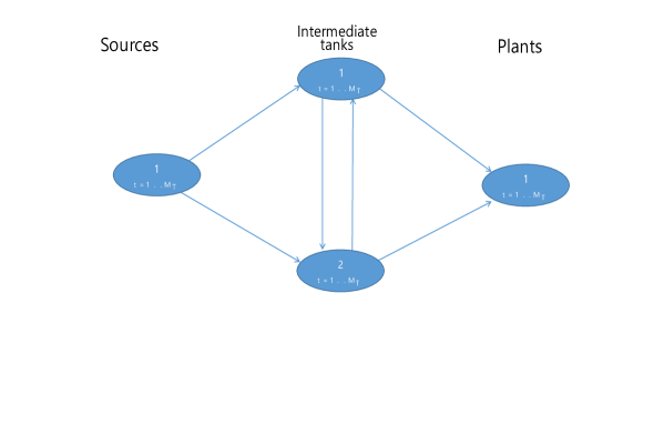
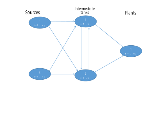
Figure 4: Instances 1, 2, 3, and 4

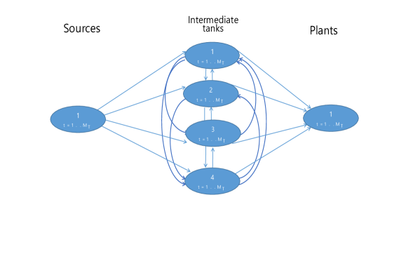
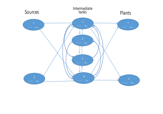
Figure 5: Instances 5, 6, 7, and 8

Table 2: $M_{S}$: the number of sources, $M_{I}$: the number of intermediate tanks, $M_{P}$: the number of plants, $(\#a,\#p,\#q,\#v)$: the numbers of variables, $|A|$: the number of pipelines, $n$: sum of all variables.

Instance	$M_{S}$	$M_{I}$	$M_{P}$	$M_{T}$	$|A|$	$\#a$	$\#p$	$\#q$	$\#v$	$n$
1	1	2	1	10	6	60	29	39	10	138
2	1	2	1	20	6	120	59	79	20	298
3	2	2	1	10	8	80	38	48	10	176
4	2	2	1	20	8	160	78	98	10	356
5	1	4	1	7	20	140	34	41	7	222
6	1	4	1	14	20	280	69	83	14	446
7	2	4	2	28	28	784	166	222	56	1228
8	2	4	2	28	28	784	166	222	56	1228
9	10	18	7	2	612	1224	46	60	14	1344
10	8	20	10	2	740	1480	48	68	20	1616
Foulds 3	11	8	16	1	160	160	0	8	0	168
Foulds 4	11	8	16	1	160	160	0	8	0	168
Foulds 5	11	4	16	1	96	96	0	4	0	100

The experimental results of each instance are summarized in Tables 3, 4 and 5. We use the following ratio to measure how much the obtained solution successfully satisfies the requirements of all nodes:

sucs.ratio $$= \left(\displaystyle\sum_{t\in T}\sum_{i\in V_{P}}RQ_{i}^{t}-\sum_{t\in T}\sum_{i\in V_{P}}v_{i}^{t}\right)\left/\displaystyle\sum_{t\in T}\sum_{i\in V_{P}}RQ_{i}^{t}\right.$$

$$= \frac{{\text{(the sum of the requirements)}}-{\text{(the sum of insuffcienct values)}}}{{\text{(the sum of requirements)}}}.$$

Note that sucs.ratio in the rescheduling method is less than $100\%$ only when the rescheduling method terminates at Step 3.6.(II)2., as it cannot meet the quality requirements. In the tables, we show sucs.ratio, the optimal values of the relaxation methods, the computed objectives values of the test instances, execution time for each relaxation, and fmincon or the rescheduling method in Section 5. Sdp.ffs.nls means applying three procedures: (i) the SDP relaxation, (ii) FFS and (iii) fmincon. Socp and Lp mean the SOCP and LP relaxation, respectively. Socp.ffs.reschd and Lp.ffs.reschd denote that the instances were solved by applying the rescheduling method including the SOCP or LP relaxation, and FFS as described in Section 5. We note that Nishi’s method employs the SDP relaxation of (3). The SDP relaxation in Sdp.ffs.nls is obtained from (4). As the number of constraints in (4) is larger than that of (3), it takes longer to solve the SDP relaxation of (4) than that of Nishi’s method. In the column “Ffs.fmincon or Ffs.reschd”, the computation time by FFS and fmincon for the methods that employ fmincon is shown. FFS took very short time and most of CPU time was consumed by fmincon in the experiments. For the rescheduling method, the computational time for the entire rescheduling method excluding the conic relaxation is shown.

Table 3 displays the results on the test instances 1-4 in [16] whose number of variables varies from $n=138$ to $n=356$. For all instances, we see in the column Total that the SOCP and LP relaxation consumed much shorter CPU time than Nishi’s method and the SDP relaxation of (4). The rescheduling method took much shorter CPU time than the nonlinear program solver fmincon. As a result, Socp.ffs.reschd and Lp.ffs.reschd show shorter total CPU time than the other methods, except for the instance 2. For the instance 2, the optimal value could be found by the SDP relaxation of (3), thus, fmincon did not take long to converge with the stopping criteria. In the column Relax, the CPU time by Socp.ffs.reschd and Lp.ffs.reschd is longer than that of Socp.ffs.nls and Lp.ffs.nls as the SOCP and LP relaxations are repeatedly solved in the rescheduling method as described in Algorithm 5.3.

For the objective values obtained by the methods in Table 3, we confirm that the SDP, SOCP and LP relaxations of (4) compute the equivalent objective values, as described in Section 4. For Socp.ffs.reschd and Lp.ffs.reschd, two values are shown for the column of Relax.obj.val to denote the objective value at the starting time and the final time, respectively, as the SOCP and LP relaxations are repeatedly solved. Socp.ffs.reschd and Lp.ffs.reschd frequently provide 100% sucs.ratio with the smallest objective values in the column of Obj.val. We observe that Socp.ffs.reschd and Lp.ffs.reschd are computationally efficient and effective to obtain smaller objective values than the other methods.

Table 3: The results for the instances 1, 2, 3, and 4. “more than 24 hours” means that the method could not provide a solution within 24 hours.

Problem	Instance 1 ($n=138$)
				CPU time (seconds)
Methods	Sucs.ratio	Relax.obj.val	Obj.val	Relax	Ffs.fmincon or Ffs.reschd	Total
Nishi’s method	$97.61\%$	$202.3$	$11243.44$	6.95	1925.17	$1932.12$
Sdp.ffs.nls	$95.70\%$	$222.5$	$19827.98$	$142.67$	$340.28$	$482.95$
Socp.ffs.nls	$97.83\%$	$222.5$	$10262.53$	$12.51$	$218.38$	$230.89$
Lp.ffs.nls	$95.27\%$	$222.5$	$21792.29$	$11.76$	$5.96$	$17.72$
Socp.ffs.reschd	$100.00\%$	$222.5,\ 122.5$	$470.00$	$30.46$	$2.05$	$32.51$
Lp.ffs.reschd	$98.34\%$	$222.5,\ 162.5$	$7944.94$	$20.29$	$1.25$	$21.54$
Problem	Instance 2 ($n=298$)
	Sucs.ratio	Relax.obj.val	Obj.val	Relax	Ffs.fmincon or Ffs.reschd	Total
Nishi’s method	$99.78\%$	$617.92$	$3058.10$	8.83	16.30	$25.13$
Sdp.ffs.nls	-	-	-	more than $24$ hours
Socp.ffs.nls	$99.74\%$	$800.00$	$3407.69$	$40.60$	$15.74$	$56.34$
Lp.ffs.nls	$99.87\%$	$800.00$	$2253.85$	$29.54$	$15.73$	$45.28$
Socp.ffs.reschd	$100.00\%$	$800.00,\ 687.06$	$1092.94$	$75.15$	$1.99$	$77.14$
Lp.ffs.reschd	$100.00\%$	$800.00,\ 687.06$	$1092.94$	$61.69$	$1.92$	$63.61$
Problem	Instance 3 ($n=176$)
	Sucs.ratio	Relax.obj.val	Obj.val	Relax	Ffs.fmincon or Ffs.reschd	Total
Nishi’s method	$98.66\%$	$181.14$	$6594.55$	$7.82$	$2866.87$	$2874.69$
Sdp.ffs.nls	$99.99\%$	$300.00$	$546.91$	$548.06$	$2856.68$	$3404.74$
Socp.ffs.nls	$80.11\%$	$300.00$	$89974.73$	$16.21$	$2885.36$	$2901.57$
Lp.ffs.nls	$99.99\%$	$300.00$	$510.81$	$14.17$	$2892.56$	$2906.73$
Socp.ffs.reschd	$100.00\%$	$300.00,\ 91.57$	$503.97$	$36.49$	$1.62$	$38.11$
Lp.ffs.reschd	$99.70\%$	$300.00,\ 55.57$	$1852.02$	$32.75$	$1.78$	$34.52$
Problem	Instance 4 ($n=356$)
	Sucs.ratio	Relax.obj.val	Obj.val	Relax	Ffs.fmincon or Ffs.reschd	Total
Nishi’s method	$96.06\%$	$728.18$	$36635.41$	13.20	7044.23	$7057.45$
Sdp.ffs.nls	-	-	-	more than $24$ hours
Socp.ffs.nls	$97.03\%$	$900.00$	$27842.37$	$77.87$	$4294.91$	$4372.78$
Lp.ffs.nls	$99.48\%$	$900.00$	$5758.37$	$58.74$	$7334.06$	$7392.80$
Socp.ffs.reschd	$100.00\%$	$900.00,\ 41.87$	$1076.34$	$186.49$	$4.28$	$190.77$
Lp.ffs.reschd	$100.00\%$	$900.00,\ 170.71$	$1062.41$	$161.04$	$5.71$	$166.75$

Table 4 shows the results for the instances 5, 6, 7, and 8 in [16] where $n$ ranges from 222 to 1228. We also see in the column Total that the CPU time spend by Socp.ffs.reschd and Lp.ffs.reschd is much shorter than the other methods. In the column of Obj.val, the smallest objective values were obtained by Lp.ffs.reschd except for the instance 5. We notice that the highest sucs.ratio leads to the smallest objective value for all instances. For the instances 7 and 8 where $n$ is large, Socp.ffs.reschd and Lp.ffs.resched achieve 100% sucs.ratio, and Lp.ffs.reschd consumed the shortest CPU time.

Table 4: The results for the instances 5, 6, 7, and 8. “more than 24 hours” means that the method could not provide a solution within 24 hours.

Problem	Instance 5 ($n=222$)
				CPU time (seconds)
Methods	Sucs.ratio	Relax.obj.val	Obj.val	Relax	Ffs.fmincon or Ffs.reschd	Total
Nishi’s method	$99.44\%$	$17.87$	$3046.25$	13.33	185.67	$198.99$
Sdp.ffs.nls	$92.59\%$	$134.00$	$35658.10$	$3239.96$	$14.54$	$3254.50$
Socp.ffs.nls	$91.60\%$	$134.00$	$40381.10$	$19.27$	$153.36$	$172.63$
Lp.ffs.nls	$92.76\%$	$134.00$	$34890.66$	$17.81$	$786.83$	$804.64$
Socp.ffs.reschd	$92.62\%$	$134.00,\ 54.00$	$35483.11$	$29.10$	$1.73$	$30.84$
Lp.ffs.reschd	$94.34\%$	$134.00,\ 54.00$	$27358.17$	$30.07$	$1.60$	$31.67$
Problem	Instance 6 ($n=446$)
	Sucs.ratio	Relax.obj.val	Obj.val	Relax	Ffs.fmincon or Ffs.reschd	Total
Nishi’s method	$95.74\%$	$186.81$	$41470.49$	33.55	18000.13	$18033.68$
Sdp.ffs.nls	-	-	-	more than $24$ hours
Socp.ffs.nls	$93.14\%$	$334.00$	$66194.84$	$102.33$	$1055.38$	$1157.71$
Lp.ffs.nls	$96.51\%$	$334.00$	$34102.63$	$80.02$	$9738.29$	$9818.31$
Socp.ffs.reschd	$96.11\%$	$334.00,\ 134.00$	$37889.83$	$189.82$	$8.90$	$198.72$
Lp.ffs.reschd	$97.85\%$	$334.00,\ 38.37$	$21272.54$	$226.01$	$8.09$	$234.10$
Problem	Instance 7 ($n=1228$)
	Sucs.ratio	Relax.obj.val	Obj.val	Relax	Ffs.fmincon or Ffs.reschd	Total
Nishi’s method	$99.51\%$	$475.33$	$7176.40$	$263.59$	$39716.96$	$39980.55$
Sdp.ffs.nls	-	-	-	more than $24$ hours
Socp.ffs.nls	$99.99\%$	$824.00$	$1649.13$	$1754.10$	$32448.45$	$34202.55$
Lp.ffs.nls	$99.99\%$	$824.00$	$1667.51$	$1368.04$	$9707.45$	$11075.49$
Socp.ffs.reschd	$100.00\%$	$824.00,\ 1916.96$	$1605.70$	$11761.98$	$674.45$	$12436.43$
Lp.ffs.reschd	$100.00\%$	$824.00,\ 1996.89$	$1599.44$	$9177.46$	$688.87$	$9866.32$
Problem	Instance 8 ($n=1228$)
	Sucs.ratio	Relax.obj.val	Obj.val	Relax	Ffs.fmincon or Ffs.reschd	Total
Nishi’s method	$98.27\%$	$458.22$	$22214.26$	$256.89$	$39443.43$	$39700.32$
Sdp.ffs.nls	-	-	-	more than $24$ hours
Socp.ffs.nls	$99.99\%$	$824.00$	$1714.70$	$1746.94$	$20929.01$	$22675.94$
Lp.ffs.nls	$99.33\%$	$824.00$	$8957.09$	$1368.09$	$39583.53$	$40951.62$
Socp.ffs.reschd	$100.00\%$	$824.00,\ 20.07$	$1636.82$	$13311.83$	$800.91$	$14112.74$
Lp.ffs.reschd	$100.00\%$	$824.00,\ 20.07$	$1634.99$	$8835.86$	$660.60$	$9496.46$

Table 5: The results for the instances 9 and 10. The instances 9 and 10 with $M_{T}=2$. “$>$ 24 hours” means that the method could not provide a solution within 24 hours.

Problem	Instance 9 ($n=1344$)
				CPU time (seconds)
	Sucs.ratio	Relax.obj.val	Obj.val	Relax	Ffs.fmincon or Ffs.reschd	Total
Nishi’s method	Fail to solve the SDP relaxation due to out-of-memory
Socp.ffs.nls	$82.83\%$	$490.05$	$81347.30$	$805.78$	$>24$ hours	$-$
Lp.ffs.nls	$91.39\%$	$490.05$	$41146.81$	$588.55$	$>24$ hours	$-$
Socp.ffs.reschd	$100.00\%$	$490.05,\ 95.12$	$657.35$	$919.18$	$112.92$	$1032.10$
Lp.ffs.reschd	$100.00\%$	$490.05,\ 94.77$	$657.35$	$674.68$	$112.96$	$787.64$
Problem	Instance 10 ($n=1616$)
				CPU time (seconds)
	Sucs.ratio	Relax.obj.val	Obj.val	Relax	Ffs.fmincon or Ffs.reschd	Total
Nishi’s method	Fail to solve the SDP relaxation due to out-of-memory
Socp.ffs.nls	$86.00\%$	$511.00$	$105842.11$	$1236.56$	$>24$ hours	$-$
Lp.ffs.nls	$89.53\%$	$511.00$	$81377.36$	$911.34$	$>24$ hours	$-$
Socp.ffs.reschd	$100.00\%$	$511.00,\ 108.87$	$759.06$	$1425.09$	$28.29$	$1453.38$
Lp.ffs.reschd	$100.00\%$	$511.00,\ 102.26$	$759.06$	$1050.38$	$30.07$	$1080.45$

Next, we tested the proposed method on the problems with the minimum number of time discretization to see how large number of variables can be solved with the proposed method. The number of sources, intermediate tanks, and plants are shown in Table 2 and the intermediate tanks in the instances 9 and 10 are connected as a complete graph shown in Figure 5. The SDP relaxations for Nishi’s method and (14) could not be solved since the sizes of the SDP relaxations were too large to handle on our computer. In Table 5, we observe that fmincon used in the methods Socp.ffs.nls and Lp.ffs.nls took long time, and could not provide a solution within 24 hours for the instances 9 and 10. On the other hand, the rescheduling method, Socp.ffs.reschd and Lp.ffs.reschd, successfully solve the problems in much shorter time. The objective values obtained by Socp.ffs.reschd and Lp.ffs.reschd are smaller than those of Socp.ffs.nls and Lp.ffs.nls, providing 100% sucs.ratio.

We tested the proposed method on Foulds 3, 4 and 5 which have the largest number of variables among the standard test problems for the pooling problem in P-formulation such as Haverly, Ben-Tal, Foulds, Adhya, and RT2. As time discretization is not used in the problems, the SDP, SOCP and LP relaxations and FFS are applied to Foulds 3, 4 and 5. Table 6 displays the numerical results on the test problems. We see that the objective value obtained by the SDP, SOCP and LP relaxations are equivalent. FFS was applied to find a feasible solution of the original pooling problem. From the CPU time spent by the SDP, SOCP and LP relaxations, we observe that the LP relaxation is most efficient. The optimal values of Foulds 3, 4 are known as -8 [15]. The proposed method finds an approximate solution of Foulds 3, 4 with $n=168$ with much shorter computational time than that in [15]. As the instances 9 and10 are much larger than Foulds 3, 4 and 5, the proposed method can be applied to larger pooling problems than the standard pooling test problems.

Table 6: Numerical results on Foulds problems

Problem	Foulds 3 $(n=168)$
Relaxation			CPU time (seconds)
	Relax.obj.val	FFS.obj.val	Relax.	Ffs	Total
Sdp.ffs	$-9.00$	$-3.82$	$317.63$	$0.81$	$318.44$
Socp.ffs	$-9.00$	$-3.82$	$9.81$	$0.45$	$10.26$
Lp.ffs	$-9.00$	$-3.82$	$8.83$	$0.43$	$9.26$
Problem	Foulds 4 $(n=168)$
	Relax.obj.val	FFS.obj.val	Relax.	Ffs	Total
Sdp.ffs	$-9.00$	$-2.64$	$300.51$	$0.44$	$300.95$
Socp.ffs	$-9.00$	$-2.64$	$10.02$	$0.44$	$10.46$
Lp.ffs	$-9.00$	$-2.64$	$9.24$	$0.44$	$9.68$
Problem	Foulds 5 $(n=100)$
	Relax.obj.val	FFS.obj.val	Relax.	Ffs	Total
Sdp.ffs	$-11.00$	$-0.83$	$23.47$	$0.45$	$23.92$
Socp.ffs	$-11.00$	$-0.83$	$6.56$	$45$	$7.01$
Lp.ffs	$-11.00$	$-0.83$	$5.97$	$0.47$	$6.42$

7 Concluding remarks

We have proposed an efficient computational method for the pooling problem with time discretization using the SOCP and LP relaxations and the rescheduling method. From the form of QCQPs for the pooling problem in [16], our formulation with time discretization has been obtained by relaxing the equality constraints into inequality constraints and introducing penalty terms in the objective function. We have shown theoretically that there exists no gap among the optimal values of the SDP, SOCP and LP relaxations of our formulation. This theoretical result can be used in other formulations of the pooling problem where only bilinear terms appear.

Computational results have been presented to show the efficiency of the proposed method over the SDP relaxations of the pooling problems and applying a nonlinear programming solver. From the numerical results, we have demonstrated that the SOCP and LP relaxations are more computationally efficient than the SDP relaxations while obtaining the same optimal value. Moreover, our proposed rescheduling method is much faster than the nonlinear programming solver fmincon and effective in obtaining a solution that satisfies all the requirements. As a result, large instances up to $n=1616$ could be solved with the LP relaxation and the rescheduling method.

As the pooling problem is a bilinear problem, it may be possible to utilize the structure [15] of the problem to further improve the computational efficiency. We hope to investigate the underlying structure of the pooling problem for solving large-scale problems.

References

- [1] IBM ILOG CPLEX user’s manual. IBM, Tech. Rep., 2015.
- [2] A. A. Ahmadi, S. Dashb, and G. Hal. Optimization over structured subsets of positive semidefinite matrices via column generation. Discrete Optim., 24:129–151, 2017.
- [3] A. A. Ahmadi and A. Majumbar. DSOS and SDSOS optimization: Lp and socp-based alternatives to sum of squares optimization. In Proceedings of the 48th Annual Conference on Information Sciences and Systems, pages 1–5, 2014.
- [4] A. A. Ahmadi and A. Majumdar. Spotless: Software for DSOS and SDSOS optimization, 2014.
- [5] M. Alfaki. Models and Solution Methods for the Pooling Problem. PhD thesis, University of Bergen, Department of Informatics, University of Bergen, March 2012.
- [6] M. Alfaki and D. Haugland. Strong formulations for the pooling problem. J. Global Optim., 56:897–916, 2013.
- [7] MOSEK ApS. The mosek optimization toolbox for matlab manual. version 7.1 (revision 28.), 2015.
- [8] G. P. Barker and D. Carlson. Cones of diagonally dominant matrices. Pacific Journal of Mathematics, 57(1):15–32, 1975.
- [9] A. Ben-Tal, G. Eiger, and V. Gershovitz. Global minimization by reducing the duality gap. Math. Program., 63(1-3):193–212, 1994.
- [10] C.E. Gounaris, R. Misener, and C.A. Floudas. Computational comparison of piecewise-linear relaxations for pooling problems. Ind. Eng. Chem. Res., 48(12):5742–5766, 2009.
- [11] C.A. Haverly. Studies of the behavior of recursion for the pooling problem. ACM SIGMAP Bull., 25:19–28, 1978.
- [12] S. Kim and M. Kojima. Second order cone programming relaxation of nonconvex quadratic optimization problems. Optim. Methods and Softw., 15(3-4):201–224, 2001.
- [13] S. Kim and M. Kojima. Exact solutions of some nonconvex quadratic optimization problems via SDP and SOCP relaxations. Comput. Optim. Appl., 26:143–154, 2003.
- [14] L. Libertu and C.C. Pantelides. An exact reformulation algorithm for large nonconvex nlps involving bilinear terms. J. Global Optim., 36(2):161–189, 2006.
- [15] A. Marandia, E. de Klerk, and J. Dahlc. Solving sparse polynomial optimization problems with chordal structure using the sparse, bounded-degree sum-of-squares hierarchy. Discrete Appl. Math., to appear, 2018.
- [16] T. Nishi. A semidefinite programming relaxation approach for the pooling problem a semidefinite programming relaxation approach for the pooling problem. Master’s thesis, Kyoto University, Department of Applied Mathematics and Physics, Kyoto University, February 2010.
- [17] J. F. Sturm. SeDuMi 1.02, a MATLAB toolbox for optimization over symmetric cones. Optim. Methods and Softw., 11&12:625–653, 1999.
- [18] R. H. Tütüncü, K. C. Toh, and M. J. Todd. Solving semidefinite-quadratic-linear programs using SDPT3. Math. Program., 95:189–217, 2003.
- [19] H. Waki, S. Kim, M. Kojima, M. Muramatsu, and H. Sugimoto. Algorithm 883: SparsePOP: a sparse semidefinite programming relaxation of polynomial optimization problems. ACM Trans. Math. Softw., 35(15), 2008.
- [20] M. Yamashita, K. Fujisawa, M. Fukuda, K. Kobayashi, K. Nakata, and M. Nakata. Latest developments in the SDPA family for solving large-scale SDPs. In Handbook on semidefinite, conic and polynomial optimization, pages 687–713. Springer, 2012.
- [21] M. Yamashita, K. Fujisawa, and M. Kojima. Implementation and evaluation of SDPA 6.0 (semidefinite programming algorithm 6.0). Optim. Methods and Softw., 18(4):491–505, 2003.
- [22] E. Zanni. Can semidefinite programming be a key approach to the pooling problem? University of Edinburgh, March 2013.