Characterizing Star-PCGs

Abstract

A graph $G$ is called a pairwise compatibility graph (PCG, for short) if it admits a tuple $(T,w,d_{\min},d_{\max})$ of a tree $T$ whose leaf set is equal to the vertex set of $G$, a non-negative edge weight $w$, and two non-negative reals $d_{\min}\leq d_{\max}$ such that $G$ has an edge between two vertices $u,v\in V$ if and only if the distance between the two leaves $u$ and $v$ in the weighted tree $(T,w)$ is in the interval $[d_{\min},d_{\max}]$. The tree $T$ is also called a witness tree of the PCG $G$. The problem of testing if a given graph is a PCG is not known to be NP-hard yet. To obtain a complete characterization of PCGs is a wide open problem in computational biology and graph theory. In literature, most witness trees admitted by known PCGs are stars and caterpillars. In this paper, we give a complete characterization for a graph to be a star-PCG (a PCG that admits a star as its witness tree), which provides us the first polynomial-time algorithm for recognizing star-PCGs.

Key words.   Pairwise Compatibility Graph; Polynomial-time Algorithm; Graph Algorithm; Graph Theory

1 Introduction

Pairwise compatibility graph is a graph class originally motivated from computational biology. In biology, the evolutionary history of a set of organisms is represented by a phylogenetic tree, which is a tree with leaves representing known taxa and internal nodes representing ancestors that might have led to these taxa through evolution. Moreover, the edges in the phylogenetic tree may be assigned weights to represent the evolutionary distance among species. Given a set of taxa and some relations among the taxa, we may want to construct a phylogenetic tree of the taxa. The set of taxa may be a subset of taxa from a large phylogenetic tree, subject to some biologically-motivated constraints. Kearney, Munro and Phillips [12] considered the following constraint on sampling based on the observation in [10]: the pairwise distance between any two leaves in the sample phylogenetic tree is between two given integers $d_{min}$ and $d_{max}$. This motivates the introduction of pairwise compatibility graphs (PCGs). Given a phylogenetic tree $T$ with an edge weight $w$ and two real numbers $d_{min}$ and $d_{max}$, we can construct a graph $G$ each vertex of which is corresponding to a leaf of $T$ so that there is an edge between two vertices in $G$ if and only if the corresponding two leaves of $T$ are at a distance within the interval $[d_{min},d_{max}]$ in $T$. The graph $G$ is called the PCG of the tuple $(T,w,d_{min},d_{max})$. Nowadays, PCG becomes an interesting graph class and topic in graph theory. Plenty of structural results have been developed.

It is straightforward to construct a PCG from a given tuple $(T,w,d_{min},d_{max})$. However, the inverse direction seems a considerably hard task. Few methods have been known for constructing a corresponding tuple $(T,w,d_{min},d_{max})$ from a given graph $G$. The inverse problem attracts certain interests in graph algorithms, which may also have potential applications in computational biology. It has been extensively studied from many aspects after the introduction of PCG [3, 6, 7, 9, 19, 18].

A natural question was whether all graphs are PCGs. This was proposed as a conjecture in [12], and was confuted in [18] by giving a counterexample of a bipartite graph with with 15 vertices. Later, a counterexample with eight vertices and a counterexample of a planar graph with 20 vertices were found [9]. It has been checked that all graphs with at most seven vertices are PCGs [3] and all bipartite graphs with at most eight vertices are PCGs [14]. In fact, it is even not easy to check whether a graph with a small constant number of vertices is a PCG or not. Whether recognizing PCGs is NP-hard or not is currently open. Some references conjecture the NP-hardness of the problem [7, 9]. A generalized version of PCG recognition is shown to be NP-hard [9].

PCG also becomes an interesting graph class in graph theory. It contains the well-studied graph class of leaf power graphs (LPGs) as a subset of instances such that $d_{min}=0$, which was introduced in the context of constructing phylogenies from species similarity data [8, 13, 15]. Another natural relaxation of PCG is to set $d_{max}=\infty$. This graph class is known as min leaf power graph (mLPG) [6], which is the complement of LPG. Several other known graph classes have been shown to be subclasses of PCG, e.g., disjoint union of cliques [2], forests [11], chordless cycles and single chord cycles [19], tree power graphs [18], threshold graphs [6], triangle-free outerplanar 3-graphs [16], some particular subclasses of split matrogenic graphs [6], Dilworth 2 graphs [5], the complement of a forest [11] and so on. It is also known that a PCG with a witness tree being a caterpillar also allows a witness tree being a centipede [4]. A method for constructing PCGs is derived [17], where it is shown that a graph $G$ consisting two graphs $G_{1}$ and $G_{2}$ that share a vertex as a cut-vertex in $G$ is a PCG if and only both $G_{1}$ and $G_{2}$ are PCGs.

How to recognize PCGs or construct a corresponding phylogenetic tree for a PCG has become an interesting open problem in this area. To make a step toward this open problem, we consider PCGs with a witness tree being a star in this paper, which we call star-PCGs. One motivation why we consider stars is that: in the literature, most of the witness trees of PCGs have simple graph structures, such as stars and caterpillars [7]. It is also fundamental to consider the problem of characterizing subclasses of PCGs derived from a specific topology of trees. Although stars are trees with a rather simple topology, star-PCG recognition is not easy at all. It is known that threshold graphs are star-PCGs (even in star-LPG and star-mLPG) and the class of star-PCGs is nearly the class of three-threshold graphs, a graph class extended from the threshold graphs [6]. However, no complete characterization of star-PCGs and no polynomial-time recognition of star-PCGs are known. In this paper, we give a complete characterization for a graph to be a star-PCG, which provides us the first polynomial-time algorithm for recognizing star-PCGs.

The main idea of our algorithm is as follows. Without loss of generality, we always rank the leaves of the witness star $T_{V}$ (and the corresponding vertices in the star-PCG $G$) according to the weight of the edges incident on it. When such an ordering of the vertices in a star-PCG $G$ is given, we can see that all the neighbors of each vertex in $G$ must appear consecutively in the ordering. This motivates us to define such an ordering to be “consecutive ordering.” To check if a graph is a star-PCG, we can first check if the graph can have a consecutive ordering of vertices. Consecutive orderings can be computed in polynomial time by reducing to the problem of recognizing interval graphs. However, this is not enough to test star-PCGs. A graph may not be a star-PCG even if it has a consecutive ordering of vertices. We further investigate the structural properties of star-PCGs on a fixed consecutive ordering of vertices. We find that three cases of non-adjacent vertex pairs, called gaps, can be used to characterize star-PCGs. A graph is a star-PCG if and only if it admits a consecutive ordering of vertices that is gap-free (Theorem 4.1). Finally, to show that whether a given graph is gap-free or not can be tested in polynomial time (Theorem 5.1), we also use a notion of “contiguous orderings.” All these together contribute to a polynomial-time algorithm for our problem.

The paper is organized as follows. Section 2 introduces some basic notions and notations necessary to this paper. Section 3 discusses how to test whether a given family $\mathcal{S}$ of subsets of an element set $V$ admits a special ordering on $V$, called “consecutive” or “contiguous” orderings and proves the uniqueness of such orderings under some conditions on $\mathcal{S}$. This uniqueness plays a key role to prove that whether a given graph is a star-PCG or not can tested in polynomial time. Section 4 characterizes the class of star-PCGs $G=(V,E)$ in terms of an ordering $\sigma$ of the vertex set $V$, called a “gap-free” ordering, and shows that given a gap-free ordering of $V$, a tuple $(T,w,d_{\min},d_{\max})$ that represents $G$ can be computed in polynomial time. Section 5 first derives structural properties on a graph that admits a “gap-free” ordering, and then presents a method for testing if a given graph is a star-PCG or not in polynomial time by using the result on contiguous orderings to a family of sets. Finally Section 6 makes some concluding remarks. Due to the space limitation, some proofs are moved to Appendix.

2 Preliminaries

For two integers $a$ and $b$, let $[a,b]$ denote the set of integers $i$ with $a\leq i\leq b$. For a sequence $\sigma$ of elements, let $\overline{\sigma}$ denote the reversal of $\sigma$. A sequence obtained by concatenating two sequences $\sigma_{1}$ and $\sigma_{2}$ in this order is denoted by $(\sigma_{1},\sigma_{2})$.

Families of Sets.

Let $V$ be a set of $n\geq 1$ elements. We call a subset $S\in V$ trivial in $V$ if $|S|\leq 1$ or $S=V$. We say that a set $X$ has a common element with a set $Y$ if $X\cap Y\neq\emptyset$. We say that two subsets $X,Y\subseteq V$ intersect (or $X$ intersects $Y$) if three sets $X\cap Y$, $X\setminus Y$, and $Y\setminus X$ are all non-empty sets. A partition $\{V_{1},V_{2},\ldots,V_{k}\}$ of $V$ is defined to be a collection of disjoint non-empty subsets $V_{i}$ of $V$ such that their union is $V$, where possibly $k=1$.

Let $\mathcal{S}\subseteq 2^{V}$ be a family of $m$ subsets of $V$. A total ordering $u_{1},u_{2},\ldots,u_{n}$ of elements in $V$ is called consecutive to $\mathcal{S}$ if each non-empty set $S\in\mathcal{S}$ consists of elements with consecutive indices, i.e., $S$ is equal to $\{u_{i},u_{i+1},\ldots,u_{i+|S|-1}\}$ for some $i\in[1,n-|S|-1]$. A consecutive ordering $u_{1},u_{2},\ldots,u_{n}$ of elements in $V$ to $\mathcal{S}$ is called contiguous if any two sets $S,S^{\prime}\in\mathcal{S}$ with $S^{\prime}\subseteq S$ start from or end with the same element along the ordering, i.e., $S^{\prime}=\{u_{j},u_{j+1},\ldots,u_{j+|S^{\prime}|-1}\}$ and $S=\{u_{i},u_{i+1},\ldots,u_{i+|S|-1}\}$ satisfy $j=i$ or $j+|S^{\prime}|=i+|S|$.

Graphs.

Let a graph stand for a simple undirected graph. A graph (resp., bipartite graph) with a vertex set $V$ and an edge set $E$ (resp., an edge set $E$ between two vertex sets $V_{1}$ and $V_{2}=V\setminus V_{1}$) is denoted by $G=(V,E)$ (resp., $(V_{1},V_{2},E)$). Let $G$ be a graph, where $V(G)$ and $E(G)$ denote the sets of vertices and edges in a graph $G$, respectively. For a vertex $v$ in $G$, we denote by $N_{G}(v)$ the set of neighbors of a vertex $v$ in $G$, and define degree $\mathrm{deg}_{G}(v)$ to be the $|N_{G}(v)|$. We call a pair of vertices $u$ and $v$ in $G$ a mirror pair if $N_{G}(v)\setminus\{u\}=N_{G}(u)\setminus\{v\}$. Let $X$ be a subset of $V(G)$. Define $N_{G}(X)$ to be the set of neighbors of $X$, i.e., $N_{G}(X)=\{u\in N_{G}(v)\setminus X\mid v\in X\}$. Let $G-X$ denote the graph obtained from $G$ by removing vertices in $X$ together with all edges incident to vertices in $X$, where $G-\{v\}$ for a vertex $v$ may be written as $G-v$. Let $G[X]$ denote the graph induced by $X$, i.e., $G[X]=G-(V(G)\setminus X)$.

Let $T$ be a tree. A vertex $v$ in $T$ is called an inner vertex if $\mathrm{dege}_{T}(v)\geq 2$ and is called a leaf otherwise. Let $L(T)$ denote the set of leaves. An edge incident to a leaf in $T$ is called a leaf edge of $T$. A tree $T$ is called a star if it has at most one inner vertex.

Weighted Graphs.

An edge-weighted graph $(G,w)$ is defined to be a pair of a graph $G$ and a non-negative weight function $w:E(G)\to\Re_{+}$. For a subgraph $G^{\prime}$ of $G$, let $w(G^{\prime})$ denote the sum $\sum_{e\in E(G^{\prime})}w(e)$ of edge weights in $G^{\prime}$.

Let $(T,w)$ be an edge-weighted tree. For two vertices $u,v\in V(T)$, let $\mathrm{d}_{T,w}(u,v)$ denote the sum of weights of edges in the unique path of $T$ between $u$ and $v$.

PCGs.

For a tuple $(T,w,d_{\min},d_{\max})$ of an edge-weighted tree $(T,w)$ and two non-negative reals $d_{\min}$ and $d_{\max}$, define $G(T,w,d_{\min},d_{\max})$ to be the simple graph $(L(T),E)$ such that, for any two distinct vertices $u,v\in L(T)$, $uv\in E$ if and only if $d_{\min}\leq\mathrm{d}_{T,w}(u,v)\leq d_{\max}$. Note that $G(T,w,d_{\min},d_{\max})$ is not necessarily connected.

A graph $G$ is called a pairwise compatibility graph (PCG, for short) if there exists a tuple $(T,w,d_{\min},d_{\max})$ such that $G$ is isomorphic to the graph $G(T,d_{\min},d_{\max})$, where we call such a tuple a pairwise compatibility representation (PCR, for short) of $G$, and call a tree $T$ in a PCR of $G$ a pairwise compatibility tree (PCT, for short) of $G$. The tree $T$ is called a witness tree of $G$. We call a PCG $G$ a star-PCG if it admits a PCR $(T,w,d_{\min},d_{\max})$ such that $T$ is a star. Fig. 1 illustrates examples of star-PCGs and PCRs of them. Although phylogenetic trees may not have edges with weight 0 or degree-2 vertices by some biological motivations [4], our PCTs do not have these constraints. This relaxation will be helpful for us to analyze structural properties of PCGs from graph theory. Furthermore, it is easy to get rid of edges with weight 0 or degree-2 vertices in a tree by contracting an edge.

Lemma 1

Every PCG admits a PCR $(T,w,d_{\min},d_{\max})$ such that $0<d_{\min}<d_{\max}$ and $w(e)>0$ for all edges $e\in E(T)$.

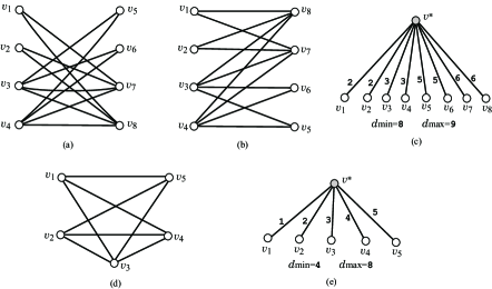
Figure 1: Illustration of examples of star-PCG. (a) A connected and bipartite star-PCG $G_{1}=(V_{1},V_{2},E)$, where ordering $\sigma_{a}=v_{1},v_{2},v_{3},v_{4},v_{8},v_{7},v_{6},v_{5}$ is not gap-free to $G_{1}$. (b) $G_{1}$ in (a) with a gap-free ordering $\sigma_{b}=v_{1},v_{2},\ldots,v_{8}$. (c) A PCR $(T,w,d_{\min}=8,d_{\max}=9)$ of $G_{1}$ in (b). (d) A connected and non-bipartite star-PCG $G_{2}$. (e) A PCR $(T,w,d_{\min}=4,d_{\max}=8)$ of $G_{2}$ in (d).

3 Consecutive/Contiguous Orderings of Elements

Let $\mathcal{S}\subseteq 2^{V}$ be a family of $m$ subsets of a set $V$ of $n\geq 1$ elements in this section. Let $V(\mathcal{S})$ denote the union of all subsets in $\mathcal{S}$, and $\pi(\mathcal{S})$ denote the partition $\{V_{1},V_{2},\ldots,V_{p}\}$ of $V(\mathcal{S})$ such that $u,v\in V_{i}$ for some $i$ if and only if $\mathcal{S}$ has no set $S$ with $|\{u,v\}\cap S|=1$. An auxiliary graph $H_{\mathcal{S}}$ for $\mathcal{S}$ is defined to be the graph $(\mathcal{S},E_{\mathcal{S}})$ that joins two sets $S,S^{\prime}\in\mathcal{S}$ with an edge $SS^{\prime}\in E_{\mathcal{S}}$ if and only if $S$ and $S^{\prime}$ intersect.

3.1 Consecutive Orderings of Elements

Observe that when $\mathcal{S}$ admits a consecutive ordering of $V(\mathcal{S})$, any subfamily $\mathcal{S}^{\prime}\subseteq\mathcal{S}$ admits a consecutive ordering of $V(\mathcal{S}^{\prime})$. We call a non-trivial set $C\subseteq V$ a cut to $\mathcal{S}$ if no set $S\in\mathcal{S}$ intersects $C$, i.e., each $S\in\mathcal{S}$ satisfies one of $S\supseteq C$, $S\subseteq C$ and $S\cap C=\emptyset$. We call $\mathcal{S}$ cut-free if $\mathcal{S}$ has no cut.

Theorem 3.1

For a set $V$ of $n\geq 1$ elements and a family $\mathcal{S}\subseteq 2^{V}$ of $m\geq 1$ sets, a consecutive ordering of $V$ to $\mathcal{S}$ can be found in $O(nm^{2})$ time, if one exists. Moreover if $\mathcal{S}$ is cut-free, then a consecutive ordering of $V$ to $\mathcal{S}$ is unique up to reversal.

3.2 Contiguous Orderings of Elements

We call two elements $u,v\in V$ equivalent in $\mathcal{S}$ if no set $S\in\mathcal{S}$ satisfies $|\{u,v\}\cap S|=1$. We call $\mathcal{S}$ simple if there is no pair of equivalent elements $u,v\in V$. Define $\mathcal{X}_{\mathcal{S}}$ to be the family of maximal sets $X\subseteq V$ such that any two vertices in $X$ are equivalent and $X$ is maximal subject to this property.

A non-trivial set $S\in\mathcal{S}$ is called a separator if no other set $S^{\prime}\in\mathcal{S}$ contains or intersects $S$, i.e., each $S^{\prime}\in\mathcal{S}$ satisfies $S^{\prime}\subseteq S$ or $S^{\prime}\cap S=\emptyset$. We call $\mathcal{S}$ separator-free in $\mathcal{S}$ if $\mathcal{S}$ has no separator.

Theorem 3.2

For a set $V$ of $n\geq 1$ elements and a family $\mathcal{S}\subseteq 2^{V}$ of $m\geq 1$ sets, a contiguous ordering of $V$ to $\mathcal{S}$ can be found in $O(nm^{2})$ time, if one exists. Moreover all elements in each set $X\in\mathcal{X}_{\mathcal{S}}$ appear consecutively in any contiguous ordering of $V$ to $\mathcal{S}$, and a contiguous ordering of $V$ to $\mathcal{S}$ is unique up to reversal of the entire ordering and arbitrariness of orderings of elements in each set $X\in\mathcal{X}_{\mathcal{S}}$.

4 Star-PCGs

Let $G=(V,E)$ be a graph with $n\geq 2$ vertices, not necessarily connected. Let $M_{G}$ denote the set of mirror pairs $\{u,v\}\subseteq V$ in $G$, i.e., $N_{G}(u)\setminus\{v\}=N_{G}(v)\setminus\{u\}$, where $u$ and $v$ are not necessarily adjacent. Let $T_{V}$ be a star with a center $v^{*}$ and $L(T)=V$. An ordering of $V$ is defined to be a bijection $\sigma:V\to\{1,2,\ldots,n\}$, and we simply write a vertex $v$ with $\sigma(v)=i$ with $v_{i}$. For an edge weight $w$ in $T_{V}$, we simply denote $w(v^{*}v_{i})$ by $w_{i}$. When $G$ is a star-PCG of a tuple $(T_{V},w,d_{\min},d_{\max})$, there is an ordering $\sigma$ of $V$ such that $w_{1}\leq w_{2}\leq\cdots\leq w_{n}$. Conversely this section derives a necessary and sufficient condition for a pair $(G,\sigma)$ of a graph $G$ and an ordering $\sigma$ of $V$ to admit a PCR $(T_{V},w,d_{\min},d_{\max})$ of $G$ such that $w_{1}\leq w_{2}\leq\cdots\leq w_{n}$.

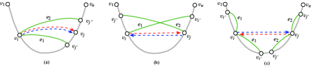
Figure 2: Illustration of a gap $\{v_{i},v_{j}\}$ in an ordered graph $G=(V=\{v_{1},v_{2},\ldots,v_{n}\},E)$: (a) $e_{1}=v_{i}v_{j^{\prime}}$ and $e_{2}=v_{i}v_{j^{\prime\prime}}$ such that $j^{\prime}<j<j^{\prime\prime}$, (b) $e_{1}=v_{i}v_{i^{\prime}}$ and $e_{2}=v_{j}v_{j^{\prime}}$ such that $j^{\prime}<i$ and $j<i^{\prime}$, (c) $e_{1}=v_{i}v_{i^{\prime}}$ and $e_{2}=v_{j}v_{j^{\prime}}$ such that $i^{\prime}<j$ and $i<j^{\prime}$, where possibly $j^{\prime}\leq i^{\prime}$ or $i^{\prime}<j^{\prime}$.

For an ordering $\sigma$ of $V$, a non-adjacent vertex pair $\{v_{i},v_{j}\}$ with $i<j$ in $G$ is called a gap (with respect to edges $e_{1},e_{2}\in E$) if there are edges $e_{1},e_{2}\in E$ that satisfy one of the following:
  (g1) $e_{1}=v_{i}v_{j^{\prime}}$ and $e_{2}=v_{i}v_{j^{\prime\prime}}$ such that $j^{\prime}<j<j^{\prime\prime}$ (or $e_{1}=v_{i^{\prime}}v_{j}$ and
     $e_{2}=v_{i^{\prime\prime}}v_{j}$ such that $i^{\prime}<i<i^{\prime\prime}$), as illustrated in Fig. 2(a);
  (g2) $e_{1}=v_{i}v_{i^{\prime}}$ and $e_{2}=v_{j}v_{j^{\prime}}$ such that $j^{\prime}<i$ and $j<i^{\prime}$, as illustrated
     in Fig. 2(b); and
  (g3) $e_{1}=v_{i}v_{i^{\prime}}$ and $e_{2}=v_{j}v_{j^{\prime}}$ such that $i^{\prime}<j$ and $i<j^{\prime}$, as illustrated
     in Fig. 2(c).
We call an ordering $\sigma$ of $V$ gap-free in $G$ if it has no gap. Clearly the reversal of a gap-free ordering of $V$ is also gap-free. We can test if a given ordering is gap-free or not in $O(n^{4})$ time by checking the conditions (a)-(c) for each non-adjacent vertex pair $\{v_{i},v_{j}\}$ in $G$.

Fig. 1(a) and (b) illustrate the same graph $G_{1}$ with different orderings $\sigma_{a}=u_{1},u_{2},\ldots,u_{8}$ and $\sigma_{b}=v_{1},v_{2},\ldots,v_{8}$, where $\sigma_{a}$ is not gap-free while $\sigma_{b}$ is gap-free.

We have the following result, which implies that a graph $G=(V,E)$ is a star-PCG if and only if it admits a gap-free ordering of $V$.

Theorem 4.1

For a graph $G=(V,E)$, let $\sigma$ be an ordering of $V$. Then there is a PCR $(T_{V},w,d_{\min},d_{\max})$ of $G$ such that $w_{1}\leq w_{2}\leq\cdots\leq w_{n}$ if and only if $\sigma$ is gap-free.

The necessity of this theorem is relatively easy to prove (see Lemma 9 in the Appendix). Next we consider the sufficiency of Theorem 4.1, which is implied by the next lemma.

Lemma 2

For a graph $G=(V,E)$, let $\sigma=v_{1},v_{2},\ldots,v_{n}$ be an gap-free ordering of $V$. There is a PCR $(T_{V},w,d_{\min},d_{\max})$ of $G$ such that $w_{1}\leq w_{2}\leq\cdots\leq w_{n}$. Such a set $\{w_{1},w_{2},\ldots,w_{n},d_{\min},d_{\max}\}$ of weights and bounds can be obtained in $O(n^{3})$ time.

Note that when two vertices $u$ and $v$ are not adjacent in a PCG $G$, there are two reasons: one is that the distance between them in the PCR $(T,w,d_{\min},d_{\max})$ is smaller than $d_{\min}$, and the other is that the distance is larger than $d_{\max}$. Before we try to assign some value to each $w_{i}$, we first detect this by coloring edges in the complete graph $K_{V}=(V,E\cup\overline{E})$ on the vertex set $V$ obtained from a graph $G$ by adding an edge between each non-adjacent vertex pair in $G$, where $\overline{E}={{V}\choose{2}}\setminus E$.

For a function $c:E\cup\overline{E}\to\{{\tt red},{\tt green},{\tt blue}\}$, we call an edge $e$ with $c(e)={\tt red}$ (resp., green and blue) a red (resp., green and blue) edge, and let $E_{\tt red}$ (resp., $E_{\tt green}$ and $E_{\tt blue}$) denote the sets of red (resp., green and blue) edges. We denote by $N_{\tt red}(v)$ the set of neighbors of a vertex $v$ via red edges. We define $N_{\tt green}(v)$ and $N_{\tt blue}(v)$ analogously.

A coloring of $G=(V,E)$ is defined to be a function $c:E\cup\overline{E}\to\{{\tt red},{\tt green},{\tt blue}\}$ such that $E_{\tt green}=E$. When an ordering $\sigma$ of $V$ is fixed, we simply write $(i,j)\in{\tt red}$ (resp., $(i,j)\in{\tt green}$ and $(i,j)\in{\tt blue}$) if an edge $v_{i}v_{j}\in E\cup\overline{E}$ is a red (resp., green and blue) edge. For $(G,\sigma)$ and a coloring $c$ of $G$, we wish to determine weights $w_{i}$, $i-1,2,\ldots,n$ and bounds $d_{\min}$ and $d_{\max}$ so that the next holds:
    $w_{1}\leq w_{2}\leq\cdots\leq w_{n}$;
    $d_{\min}\leq w_{i}+w_{j}\leq d_{\max}$ for $(i,j)\in{\tt red}$;
    $w_{i}+w_{j}<d_{\min}$ for $(i,j)\in{\tt green}$; and
    $w_{i}+w_{j}>d_{\max}$ for $(i,j)\in{\tt blue}$.
To have such a set $\{w_{1},\ldots,w_{n},d_{\min},d_{\max}\}$ of values for an ordering $\sigma$ and a coloring $c$ of $G$, the coloring $c$ must satisfy the following conditions:
each $v_{i}\in V$ admits integers $a(i),b(i)\in[1,n]$ such that

$$N_{\tt red}(v_{i})=\{v_{j}\mid 1\leq j\leq a(i)-1\}\setminus\{v_{i}\} N_{\tt blue}(v_{i})=\{v_{j}\mid b(i)+1\leq j\leq n\}\setminus\{v_{i}\}$$ and ,

where $a(i)=1$ if $N_{\tt red}(v_{i})=\emptyset$; $b(i)=n$ if $N_{\tt blue}(v_{i})=\emptyset$; and $N_{\tt green}(v_{i})=V\setminus(N_{\tt red}(v_{i})\cup N_{\tt blue}(v_{i})\cup\{v_{i}\})=\{v_{j}\mid a(i)\leq j\leq b(i)\}\setminus\{v_{i}\}\setminus\{v_{i}\}$, and $N_{\tt green}(v_{i})=\emptyset$ if $b(i)<a(i)$. Such a coloring $c$ of $G$ is called proper to $(G,\sigma)$.

Lemma 3

For a graph $G=(V,E)$ and a gap-free ordering $\sigma$ of $V$, there is a coloring $c$ of $G$ that is proper to $(G,\sigma)$, which can be found in in $O(n^{2})$ time.

Define integers $i_{\tt red}$ and $i_{\tt blue}$ as follows.

$$i_{\tt red}=\left\{\begin{array}[]{cc}\mbox{the largest index $i$ such that $i<a(i)$}&\mbox{ if $E_{\tt red}\neq\emptyset$},\\ 0&\mbox{ if $E_{\tt red}=\emptyset$},\end{array}\right.$$

$$i_{\tt blue}=\left\{\begin{array}[]{cc}\mbox{the smallest index $i$ such that $b(i)<i$}&\mbox{ if $E_{\tt blue}\neq\emptyset$},\\ n+1&\mbox{ if $E_{\tt blue}=\emptyset$}.\end{array}\right.$$

In other words, $i_{\tt red}\neq 0$ is the largest $i$ with $(i,i+1)\in{\tt red}$, and $i_{\tt red}<n$, whereas $i_{\tt blue}\neq n+1$ is the smallest $i$ with $(i-1,i)\in{\tt blue}$, and $i_{\tt blue}>1$. Given a graph $G$, a gap-free ordering $\sigma=v_{1},v_{2},\ldots,v_{n}$ of $V$, and a coloring $c$ proper to $(G,\sigma)$, we can find the set $\{a(i),b(i)\mid i=1,2,\ldots,n\}\cup\{i_{\tt red},i_{\tt blue}\}$ of indices in $O(n^{2})$ time. We also compute the set $M_{G}$ of all mirror pairs in $O(n^{3})$ time. Equipped with above results, we can prove the sufficiency of Theorem 4.1 by designing an $O(n)$-time algorithm that assigns the right values to weights $w_{1},w_{2},\ldots,w_{n}$ in $T_{V}$. The details can be found in Appendix 0.E.

5 Recognizing Star-PCGS

Based on Theorem 4.1, we can test whether a graph $G=(V,E)$ is a star-PCG or not by generating all $n!$ orderings of $V$. In this section, we show that testing whether a graph has a gap-free ordering of $V$ can be tested in polynomial time.

Theorem 5.1

Whether a given graph $G=(V,E)$ with $n$ vertices has a gap-free ordering of $V$ can be tested in $O(n^{6})$ time.

In a graph $G=(V,E)$, let $E^{\tt t}$ denote the union of edge sets of all cycles of length 3 in $G$, $V^{\tt t}$ denote the set of end-vertices of edges in $E^{\tt t}$, and $N_{G}^{\tt t}(v)$ denote the set of neighbors $u\in N_{G}(v)$ of a vertex $v\in V$ such that $uv\in E^{\tt t}$.

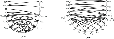
Figure 3: (a) A disconnected graph $G=(V,E)$, (b) A connected non-bipartite graph $G=(V,E)$, where the edges between two vertices in $V^{*}=\{u_{7},u_{8},u_{9},u_{10},u_{11},u_{12},u_{13},u_{14}\}$ are not depicted.

Lemma 4

For a graph $G=(V,E)$ with a gap-free ordering $\sigma=v_{1},v_{2},\ldots,v_{n}$ of $V$ and a coloring $c$ proper to $\sigma$, let $V_{1}=\{v_{i}\mid 1\leq i\leq i_{\tt red}\}$, $V_{2}=\{v_{i}\mid i_{\tt blue}\leq i\leq n\}$, and $V^{*}=\{v_{i}\mid i_{\tt red}-1\leq i\leq i_{\tt blue}+1\}$. Then

1. If two edges $v_{i}v_{j}$ and $v_{i^{\prime}}v_{j^{\prime}}$ with $i<j$ and $i^{\prime}<j^{\prime}$ cross $($i.e., $i<i^{\prime}<j<j^{\prime}$ or $i^{\prime}<i<j^{\prime}<j)$, then they belong to the same component of $G$;

2. It holds $i_{\tt red}+1\leq i_{\tt blue}-1$. The graph $G[V^{*}]$ is a complete graph, and $G-V^{*}$ is a bipartite graph between vertex sets $V_{1}$ and $V_{2}$;

3. Every two vertices $v_{i},v_{j}\in V_{1}\cap N_{G}(V^{*})$ with $i<j$ satisfy $v_{i_{\tt blue}-1}\in N_{G}(v_{i})\cap V^{*}\subseteq N_{G}(v_{j})\cap V^{*}\subseteq V^{*}\setminus\{v_{i_{\tt red}+1}\}$; and
   Every two vertices $v_{i},v_{j}\in V_{2}\cap N_{G}(V^{*})$ with $i<j$ satisfy $v_{i_{\tt red}+1}\in N_{G}(v_{j})\cap V^{*}\subseteq N_{G}(v_{i})\cap V^{*}\subseteq V^{*}\setminus\{v_{i_{\tt blue}-1}\}$.

We call the complete graph $G[V^{*}]$ in Lemma 4(ii) the core of $G$. Based on the next lemma, we can treat each component of a disconnected graph $G$ separately to test whether $G$ is a star-PCG or not.

Lemma 5

Let $G=(V,E)$ be a graph with at least two components.

1. If $G$ admits a gap-free ordering of $V$, then each component of $G$ admits a gap-free ordering of its vertex set, and there is at most one non-bipartite component in $G$; and

2. Let $G^{\prime}=(V^{\prime}_{1},V^{\prime}_{2},E^{\prime})$ be a bipartite component of $G$, and $G^{\prime\prime}=G-V(G^{\prime})$. Assume that $G^{\prime}$ admits a gap-free ordering $v^{\prime}_{1},v^{\prime}_{2},\ldots,v^{\prime}_{p}$ of $V^{\prime}_{1}\cup V^{\prime}_{2}$ and $G^{\prime\prime}$ admits a gap-free ordering $v_{1},v_{2},\ldots,v_{q}$ of $V_{2}$. Then there is an index $k$ such that $\{\{v^{\prime}_{1},v^{\prime}_{2},\ldots,v^{\prime}_{k}\},\{v^{\prime}_{k+1},v^{\prime}_{k+2},\ldots,v^{\prime}_{p}\}\}=\{V^{\prime}_{1},V^{\prime}_{2}\}$. Moreover, the ordering $v^{\prime}_{1},v^{\prime}_{2},\ldots,v^{\prime}_{k},v_{1},v_{2},\ldots,v_{q},v^{\prime}_{k+1},v^{\prime}_{k+2},\ldots,v^{\prime}_{p}$ of $V$ is gap-free to $G$.

Proof. (i) Let $G$ admit a gap-free ordering of $V$. Any induced subgraph $G$ such as a component of $G$ is a star-PCG, and a gap-free ordering of its vertex set by Theorem 4.1. By Lemma 4(i), at most one component $H$ containing a complete graph with at least three vertices can be non-bipartite, and the remaining graph $G-V(H)$ must be a collection of bipartite graphs.

(ii) Immediate from the definition of gap-free orderings. ∎

We first consider the problem of testing if a given connected bipartite graph is a star-PCG or not. We reduce this to the problem of finding contiguous ordering to a family of sets. For a bipartite graph $G=(V_{1},V_{2},E)$, define $\mathcal{S}_{i}$ to be the family $\{N_{G}(v)\mid v\in V_{j}\}$ for the $j\in\{1,2\}-\{i,j\}$, where even if there are distinct vertices $u,v\in V_{j}$ with $N_{G}(u)=N_{G}(v)$, $\mathcal{S}_{i}$ contains exactly one set $S=N_{G}(u)=N_{G}(v)$.

For the example of a connected bipartite graph $G_{1}=(V_{1},V_{2},E)$ in Fig. 1(a), we have $\mathcal{S}_{1}=\{\{v_{3},v_{4}\},\{v_{1},v_{2},v_{3},v_{4}\}\}$, and $\mathcal{S}_{2}=\{\{v_{5},v_{6}\},\{v_{5},v_{6},v_{7},v_{8}\}\}$.

Lemma 6

Let $G=(V_{1},V_{2},E)$ be a connected bipartite graph with $|E|\geq 1$. Then family $\mathcal{S}_{i}$ is separator-free for each $i=1,2$, and $G$ has a gap-free ordering of $V$ if and only if for each $i=1,2$, family $\mathcal{S}_{i}$ admits a contiguous ordering $\sigma_{i}$ of $V_{i}$. For any contiguous ordering $\sigma_{i}$ of $V_{i}$, $i=1,2$, one of orderings $(\sigma_{1},\sigma_{2})$ and $(\sigma_{1},\overline{\sigma_{2}})$ of $V$ is a gap-free ordering to $G$.

Note that $|\mathcal{S}_{1}|+|\mathcal{S}_{2}|+|V(\mathcal{S}_{1})|+|V(\mathcal{S}_{2})|=O(n)$. By Theorem 3.2, a contiguous ordering of $V(\mathcal{S}_{i})$ for each $i=1,2$ can be computed in $O(|V(\mathcal{S}_{i})||\mathcal{S}_{i}|^{2})=O(n^{3})$ time.

Fig. 1(a) illustrates an ordering $\sigma_{a}=v_{1},v_{2},v_{3},v_{4},v_{8},v_{7},v_{6},v_{5}$ of $V(G_{1})$ of a connected bipartite graph $G_{1}=(V_{1},V_{2},E)$, where $\sigma_{a}$ consists of a contiguous ordering $\sigma_{1}=v_{1},v_{2},v_{3},v_{4}$ of $V_{1}$ and a contiguous ordering $\sigma_{2}=v_{8},v_{7},v_{6},v_{5}$ of $V_{2}$. Although $\sigma_{a}$ is not gap-free in $G$, the other ordering $\sigma_{b}$ of $V(G_{1})$ that consists of $\sigma_{1}$ and the reversal of $\sigma_{2}$ is gap-free, as illustrated in Fig. 1(b).

Finally we consider the case where a given graph $G$ is a connected and non-bipartite graph. Fig. 1(d) illustrates a connected and non-bipartite star-PCG whose maximum clique is not unique.

Lemma 7

For a connected non-bipartite graph $G=(V,E)$ with $V^{\tt t}\neq\emptyset$, and let $v^{*}_{1},v^{*}_{2}$ be two adjacent vertices in $V^{\tt t}$. Let $V^{*}=\{v^{*}_{1},v^{*}_{2}\}\cup(N_{G}(v^{*}_{1})\cap N_{G}(v^{*}_{2}))$, $V^{\prime}_{1}=N_{G}(v^{*}_{2})\setminus V^{*}$, and $V^{\prime}_{2}=N_{G}(v^{*}_{1})\setminus V^{*}$. Assume that $G$ has a gap-free ordering $\sigma$ of $V$ and a proper coloring $c$ to $\sigma$ such that $v^{*}_{1}=v_{i_{\tt red}+1}$, $v^{*}_{2}=v_{i_{\tt blue}-1}$. Then:

1. A maximal clique $K_{v^{*}_{1},v^{*}_{2}}$ of $G$ that contains edge $v^{*}_{1},v^{*}_{2}$ is uniquely given as $G[V^{*}]$. The graph $G[V^{*}]$ is the core of the ordering $\sigma$, and $G-V^{*}$ is a bipartite graph $(V_{1},V_{2},E^{\prime})$; and

2. Let $\mathcal{S}_{i}$ denote the family $\{N_{G}(v)\mid v\in V_{j}\}$ for $\{i,j\}=\{1,2\}$, and $\mathcal{S}=\mathcal{S}_{1}\cup\mathcal{S}_{2}\cup\{V^{*}\}$. Then $\mathcal{S}$ is a separator-free family that admits a contiguous ordering $\sigma$ of $V$, and any contiguous ordering $\sigma$ of $V$ is a gap-free ordering to $G$.

For example, when we choose vertices $v^{*}_{1}=u_{7}$ and $v^{*}_{2}=u_{14}$ in the connected non-bipartite graph $G=(V,E)$ in Fig. 3(b), we have $V^{*}=\{u_{7},u_{8},u_{9},u_{10},u_{11},$ $u_{12},u_{13},u_{14}\}$, $\mathcal{S}_{1}=\{\{u_{1},u_{2}\},$ $\{u_{2},u_{3},u_{4}\},\{u_{3},u_{4},u_{5}\},$ $\{u_{3},u_{4},u_{5},u_{6},u_{7},u_{8}\},$ $\{u_{5},u_{6},u_{7},u_{8},u_{9},u_{10},u_{11}\}\}$, and $\mathcal{S}_{2}=\{\{u_{19}\},$ $\{u_{18},u_{19}\},\{u_{16},u_{17},u_{18}\},$ $\{u_{13},$ $u_{14},u_{15},u_{16},u_{17}\},$ $\{u_{10},u_{11},u_{12},u_{13},u_{14},u_{15},u_{16}\}\}$.

For a fixed $V^{*}$ in Lemma 7, we can test whether the separator-free family $\mathcal{S}$ in Lemma 7(ii) is constructed from $V^{*}$ in $O(|V(\mathcal{S})||\mathcal{S}|^{2})=O(n^{3})$ time by Theorem 3.2, since $|\mathcal{S}|+|V(\mathcal{S})|=O(n)$ holds. It takes $O(n^{4})$ time to check a given ordering is gap-free or not. To find the right choice of a vertex pair $v^{*}_{1}=v_{i_{\tt red}+1}$ and $v^{*}_{2}=v_{i_{\tt blue}-1}$ of some gap-free ordering $\sigma$ of $V$, we need to try $O(n^{2})$ combinations of vertices to construct $V^{*}$ according to the lemma. Then we can find a gap-free ordering of a given graph, if one exists in $O(n^{6})$ time, proving Theorem 5.1.

By Theorems 4.1 and 5.1, we conclude that whether a given graph with $n$ vertices is a star-PCG or not can be tested in $O(n^{6})$ time.

6 Concluding Remarks

Pairwise compatibility graphs were initially introduced from the context of phylogenetics in computational biology and later became an interesting graph class in graph theory. PCG recognition is a hard task and we are still far from a complete characterization of PCG. Significant progresses toward PCG recognition would be interesting from a graph theory perspective and also be helpful in designing sampling algorithms for phylogenetic trees. In this paper, we give the first polynomial-time algorithm to recognize star-PCGs. Although stars are trees of a simple topology, it is not an easy task to recognize star-PCGs. For further study, it is an interesting topic to study the characterization of PCGs with witness trees of other particular topologies.

Appendix

Appendix 0.A Proof of Lemma 1

Lemma 1 Every PCG admits a PCR $(T,w,d_{\min},d_{\max})$ such that $0<d_{\min}<d_{\max}$ and for all edges $e\in E(T)$.

Proof. Since the case where a given PCG $G$ has at most two vertices is trivial, we assume that $G$ has at least three vertices. Let $(T,w^{\prime},d^{\prime}_{\min},d^{\prime}_{\max})$ be a PCR of $G$, where each path between two leaves in $T$ contains exactly two leaf edges since $|L(T)|=|V(G)|\geq 3$. We increase some values of $w^{\prime}(e)$, $e\in E(T)$ and $d^{\prime}_{\min}$ and $d^{\prime}_{\max}$ so that the resulting tuple satisfies the lemma. For two positive reals $\delta$ and $\varepsilon<\min_{uv\not\in E}\mathrm{d}_{T,w^{\prime}}(u,v)-d^{\prime}_{\max}$, let $w(e):=w^{\prime}(e)+\delta$ for each leaf edge $e\in E(T)$, $w(e):=w^{\prime}(e)$ for all non-leaf edges $e\in E(T)$, $d_{\min}:=d^{\prime}_{\min}+2\delta$, and $d_{\max}:=d^{\prime}_{\max}+2\delta+\varepsilon$. We observe that $(T,w,d_{\min},d_{\max})$ is a PCR of $G$ satisfying the lemma because each path between two leaves in $T$ contains exactly two leaf edges ∎

Appendix 0.B Proof of Theorem 3.1

First we prove the time complexity of the theorem. A graph $H$ with $n\geq 1$ vertices is called an interval graph if each vertex $v\in V(H)$ can represented by an ordered pair $(a_{v},b_{v})$ of reals $a_{v}\leq b_{v}$ so that two vertices $u,v\in V(H)$ are adjacent if and only if there is a real $c$ such that two intervals $a_{u}\leq c\leq b_{u}$ and $a_{v}\leq c\leq b_{v}$. It is know that testing if a given graph $H$ is an interval graph and finding such a representation $(a_{v},b_{v})$, $v\in V(H)$, if one exists can be done in $O(|V(H)|+|E(H)|)$ time [1]. Given a family $\mathcal{S}\subseteq 2^{V}$, we see that $\mathcal{S}$ admits a consecutive ordering if and only if the auxiliary graph $H_{\mathcal{S}}$ for $\mathcal{S}$ is an interval graph by the definition of $H_{\mathcal{S}}$. The time to construct $H_{\mathcal{S}}$ from $\mathcal{S}$ is $O(nm^{2})$ since we can check in $O(n)$ time whether two sets $S,S^{\prime}\in\mathcal{S}$ intersect, i.e., vertices $S,S^{\prime}\in V(H)$ are adjacent in $H$. Clearly $|V(H)|=|\mathcal{S}|=m$ and $|E(H)|\leq|\mathcal{S}|^{2}=O(m^{2})$. Then testing if $H_{\mathcal{S}}$ is an interval graph and finding a representation $(a_{v},b_{v})$, $v\in V(H)$ can be done in $O(n+m^{2})$ time. In total, it takes $O(nm^{2})$ time to find a consecutive ordering for $\mathcal{S}$, if one exits.

Next we prove that a consecutive ordering of $V$ to a cut-free family $\mathcal{S}$ is unique up to reversal. Assume that $\mathcal{S}$ admits another consecutive ordering $\tau\not\in\{\sigma,\overline{\sigma}\}$ to derive a contradiction that $\mathcal{S}$ would have a cut. Since $\tau\not\in\{\sigma,\overline{\sigma}\}$, some two elements $a,b\in V$ appear consecutively in $\sigma$, but another element $c\in V\setminus\{a,b\}$ appears in the subsequence $\tau_{ab}$ of $\tau$ between $a$ and $b$. Hence $a=v_{k}$, $b=v_{k+1}$ and $c=v_{p}$ for $\sigma=v_{1},v_{2},\ldots,v_{n}$, where $k+1<p$ is assumed without loss of generality and $c=v_{p}$ is chosen from $\tau_{ab}$ so that the index $p$ is maximized. We claim that the set $C=\{v_{k+1},v_{k+2},\dots,v_{p}\}$ is a cut to $\mathcal{S}$. To derive a contradiction, $C$ intersects a set $S\in\mathcal{S}$, where $S=\{v_{s},v_{s+1},\ldots,v_{t}\}$ for $s\leq k<k+1\leq t<p$ or $k+1<s\leq p<t$ by the consecutiveness of $S$ in $\sigma$. In the former, $S$ with $a,b\in S$ contains $\tau_{ab}$, implying $c=v_{p}\in S$, a contradiction. In the latter, $S$ is contained in $\tau_{ab}$, since $a,b\not\in S$ and $c\in S$, implying that $v_{t}$ with $p<t$ belongs to $\tau_{ab}$, a contradiction to the choice of $c=v_{p}$.

Appendix 0.C Proof of Theorem 3.2

To prove Theorem 3.2, we show that an instance $(V,\mathcal{S})$ of the problem of finding a contiguous ordering of $V$ to $\mathcal{S}$ can be modified to an instance $(V,\mathcal{S}^{\prime})$ of the problem of finding a consecutive ordering of $V$ to $\mathcal{S}^{\prime}$ by introducing some new subsets of $V$.

A set $S\in\mathcal{S}$ is called minimal (resp., maximal) if $\mathcal{S}$ contains no proper subset (resp., superset) of $S$. Define $\mathcal{S}_{\min}$ (resp., $\mathcal{S}_{\max}$) to be the family of minimal (resp., maximal) sets in $\mathcal{S}$.

Theorem 3.2 follows from (iv) and (v) of the next lemma.

Lemma 8

For a set $V$ of $n\geq 1$ elements, let $\mathcal{S}\subseteq 2^{V}\setminus\{\emptyset\}$ be a family with $m\geq 1$ sets.

1. If some set $B\in\mathcal{S}_{\max}$ contains at least three sets from $\mathcal{S}_{\min}$, then $\mathcal{S}$ cannot have a contiguous ordering of $V$;

2. Assume that $\mathcal{S}$ is separator-free. Let $X$ be a maximal set of elements any two of which are equivalent. Then the elements in $X$ appear consecutively in any contiguous ordering of $V$ to $\mathcal{S}$;

3. Assume that $\mathcal{S}$ is simple and separator-free. Let $\mathcal{S}^{\prime}$ denote the family obtained from $\mathcal{S}$ by adding a new set $S_{A,B}=B\setminus A$ for each pair of sets $A\in\mathcal{S}_{\min}$ and $B\in\mathcal{S}_{\max}$ such that $A\subsetneq B$ and $B\setminus A\not\in\mathcal{S}$. Then $\mathcal{S}^{\prime}$ is cut-free and any consecutive ordering of $V$ to $\mathcal{S}^{\prime}$ is a contiguous ordering of $V$ to $\mathcal{S}$; and

4. Assume that $\mathcal{S}$ is separator-free. Then a contiguous ordering of $V$ to $\mathcal{S}$ can be found in $O(nm^{2})$ time, if one exists. Moreover all elements in each set $X\in\mathcal{X}_{\mathcal{S}}$ appear consecutively in any contiguous ordering of $V$ to $\mathcal{S}$, and a contiguous ordering of $V$ to $\mathcal{S}$ is unique up to reversal of the entire ordering and arbitrariness of orderings of elements in each set $X\in\mathcal{X}_{\mathcal{S}}$; and

5. A contiguous ordering of $V$ to $\mathcal{S}$ can be found in $O(nm^{2})$ time, if one exists.

Proof. (i) Let three sets $A_{i}\in\mathcal{S}_{\min}$, $i=1,2,3$ be contained in some set $B\in\mathcal{S}_{\max}$. Note that each $A_{i}$ is a proper subset of $B$, and no set $A_{i}$ is contained in any other set $A_{j}$ with $j\neq i$. Hence in any contiguous ordering of $V$ to $\mathcal{S}$, at least one of the three sets $A_{i}$, $i=1,2,3$ cannot share the first element in $B$ or the last element in $B$. This means that $\mathcal{S}$ cannot have a contiguous ordering of $V$.

(ii) To derive a contradiction, assume that there is a contiguous ordering $u_{1},u_{2},\ldots,u_{n}$ of $V$ to $\mathcal{S}$ wherein the indices of elements $X$ are not consecutive, i.e., there are elements $u_{i},u_{j},u_{k}\in V$ with $i<j<k$ and a set $S\in\mathcal{S}$ such that $\{u_{i},u_{j},u_{k}\}\cap S=\{u_{j}\}$. Since $\mathcal{S}$ is separator-free, there is a set $S^{\prime}\in\mathcal{S}$ that intersects $S$ or contains $S$. Since any two elements in $X$ are equivalent, it holds that either $X\subseteq S^{\prime}$ or $X\cap S^{\prime}=\emptyset$. If $S^{\prime}$ intersects $S$, then $S^{\prime}\setminus S\neq\emptyset$ means that $S^{\prime}\supseteq X$ and $S^{\prime}$ would contain $S$ too since the indices of elements in $S^{\prime}$ are consecutive in the ordering. Hence $S^{\prime}$ always contains $S$, and it also contains $X$, where $S^{\prime}\setminus S\supseteq X$. Now $S$ does not contain the first element or the last element of $S^{\prime}$ in the ordering. This contradicts that the ordering is contiguous to $\mathcal{S}$.

(iii) For any two sets $A\in\mathcal{S}_{\min}$ and $B\in\mathcal{S}_{\max}$ such that $A\subseteq B$ and $B\setminus A\neq\emptyset$, the set $B\setminus A$ must consist of elements with consecutive indices in a contiguous ordering of $V$ to $\mathcal{S}$. Hence after adding such a set $B\setminus A$ to $\mathcal{S}$, the contiguous ordering of $V$ to $\mathcal{S}$ is a consecutive ordering of $V$ to $\mathcal{S}^{\prime}$. We show that any consecutive ordering of $V$ to $\mathcal{S}^{\prime}$ is a contiguous ordering of $V$ to $\mathcal{S}^{\prime}$. Assume that, for a consecutive ordering $u_{1},u_{2},\ldots,u_{n}$ of $V$ to $\mathcal{S}^{\prime}$, there are sets $X,Y\in\mathcal{S^{\prime}}$ such that $X\subseteq Y=\{u_{i},u_{i+1},\ldots,u_{i+|Y|-1}\}$ but $X$ does not contain any of $u_{i}$ and $u_{i+|Y|-1}$. Let $A_{X}\in\mathcal{S}_{\min}$ be a set such that $A_{X}\subseteq X$ and let $B_{Y}\in\mathcal{S}_{\max}$ be a set such that $Y\subseteq B_{Y}$. Note that $\mathcal{S^{\prime}}$ contains $B_{Y}\setminus A_{X}$, where $u_{i},u_{i+|Y|-1}\in B_{Y}\setminus A_{X}$. However $B_{Y}\setminus A_{X}$ does not consist of elements with consecutive indices in a the consecutive ordering $u_{1},u_{2},\ldots,u_{n}$, a contradiction. Hence any consecutive ordering of $V$ to $\mathcal{S}^{\prime}$ is a contiguous ordering of $V$ to $\mathcal{S}^{\prime}$.

We next prove that $\mathcal{S}^{\prime}$ is cut-free. Let $C$ be a non-trivial subset of $V$, and assume that no set $\mathcal{S}$ intersects $C$. Since $|C|\geq 2$ and $\mathcal{S}$ is simple, there is a set $S\in\mathcal{S}$ such that $S\cap C\neq\emptyset\neq C\setminus S$. If $S\setminus C\neq\emptyset$, then $S$ would intersect $C$. Hence $S\setminus C$. If each set $S^{\prime}\in\mathcal{S}$ with $S^{\prime}\cap(V\setminus C)\neq\emptyset$ is disjoint with $C$, then this would contradict that $\mathcal{S}$ is separator-free. Hence there is a set $S^{\prime}\in\mathcal{S}$ with $S^{\prime}\cap(V\setminus C)\neq\emptyset$ and $S^{\prime}\supseteq C$. After the above procedure, the resulting family $\mathcal{S}^{\prime}$ contains a set $S^{\prime\prime}$ such that $S\setminus S^{\prime\prime}\neq\emptyset$ and $S^{\prime\prime}\subseteq S^{\prime}\setminus S$, where $C\cap S^{\prime\prime}\supseteq C\setminus S\neq\emptyset$, $C\setminus S^{\prime\prime}\supseteq S\setminus S^{\prime\prime}\neq\emptyset$, and $S^{\prime\prime}\setminus C\supseteq S^{\prime}\cap(V\setminus C)\neq\emptyset$. Therefore $S^{\prime\prime}$ intersects $C$. This proves that $\mathcal{S}^{\prime}$ is cut-free.

(iv) Let $\mathcal{S}_{0}\subseteq 2^{V}$ be a given separator-free family with $m\geq 1$ subsets. First we compute the family $\mathcal{X}_{\mathcal{S}_{0}}$ of all maximal subsets. This takes $O(nm^{2})$ time. By (ii) of this lemma, all elements in each $X\in\mathcal{X}_{\mathcal{S}_{0}}$ appear consecutively in any contiguous ordering of $V$. Next we construct a simple family $\mathcal{S}$ from $\mathcal{S}_{0}$ as follows. For each set $X\in\mathcal{X}_{\mathcal{S}_{0}}$, we choose one element $v_{X}$ from $X$ and replace $X$ with $X\setminus\{u_{X}\}$ in the family. Note that the resulting family $\mathcal{S}$ is simple and separator-free and $|\mathcal{S}|\leq|\mathcal{S}_{0}|$. If $\mathcal{S}_{0}$ admits a contiguous ordering of $V$ then so does $\mathcal{S}$. For the family $\mathcal{S}$, we then compute the families $\mathcal{S}_{\min}$ and $\mathcal{S}_{\max}$ and construct a bipartite graph $\mathcal{B}=(\mathcal{S}_{\min},\mathcal{S}_{\max},E^{*})$ such that for each pair of sets $A\in\mathcal{S}_{\min}$, $B\in\mathcal{S}_{\max}$, $AB\in E^{*}$ if and only if $A\subseteq B$. This also can be done in $O(nm^{2})$ time. Now testing whether there is a set $B\in\mathcal{S}_{\max}$ satisfying the condition (i) of this lemma can be done in $O(m^{2}n)$ time, because a set $B\in\mathcal{S}_{\max}$ contains three sets in $\mathcal{S}_{\min}$ if and only if the degree of vertex $B\in\mathcal{S}_{\max}$ in $\mathcal{B}$ is at least 3. When there exists such a set $B\in\mathcal{S}_{\max}$, we conclude that $\mathcal{S}_{0}$ does not admits any contiguous ordering of $V$. Assume that no set $B\in\mathcal{S}_{\max}$ satisfies the condition (i) of this lemma, and construct from $\mathcal{S}$ the cut-free family $\mathcal{S}^{\prime}$ in (iii) of this lemma, where we see that $|\mathcal{S}^{\prime}|\leq|\mathcal{S}|+2|\mathcal{S}_{\max}|\leq 3m$. By Theorem 3.1 applied to $\mathcal{S}^{\prime}$, we can find a consecutive ordering $\sigma$ of $V(\mathcal{S}^{\prime})$ to the cut-free family $\mathcal{S}^{\prime}$ in $O(m^{2}n)$ time, if one exists, where $\sigma$ is unique up to reversal. By (iii) of this lemma,, the ordering $\sigma$ is contiguous to $\mathcal{S}$. All contiguous orderings of $V$ to the input separator-free family $\mathcal{S}_{0}$ can be obtained by replacing the representative element $v_{X}$ in $\sigma$ for each set $X\in\mathcal{X}_{\mathcal{S}_{0}}$ with an arbitrary ordering of $X$. Therefore a contiguous ordering $\sigma^{*}$ of $V$ to $\mathcal{S}_{0}$ can be found in $O(nm^{2})$ time, if one exists, and $\sigma^{*}$ is unique up to reversal and arbitrariness of orderings of elements in each set $X\in\mathcal{X}_{\mathcal{S}_{0}}$.

(v) Given a family $\mathcal{S}\subseteq 2^{V}$, we can test in $O(nm)$ time if a set $X\in\mathcal{S}$ is a cut of $\mathcal{S}$, i.e., $X$ does not intersect any other set $S\in\mathcal{S}\setminus\{X\}$. Then the family $\mathcal{C}_{\mathcal{S}}$ of all cuts of $\mathcal{S}$ can be found in $O(nm^{2})$ time, where $|\mathcal{C}_{\mathcal{S}}|\leq 2n$ since $\mathcal{C}_{\mathcal{S}}$ is a laminar. Note that any inclusion-wise maximal set in $\mathcal{C}_{\mathcal{S}}$ is a separator of $\mathcal{S}$. For each cut $X\in\mathcal{C}_{\mathcal{S}}$, let $\mathcal{C}(X)$ denote the family of sets $Y\in\mathcal{C}_{\mathcal{S}}$ such that $Y\subsetneq X$ and $Y$ is maximal, i.e., no other set $S\in\mathcal{C}_{\mathcal{S}}$ satisfies $Y\subsetneq S\subsetneq X$. For each set $X\in\mathcal{C}_{\mathcal{S}}$, let $\mathcal{S}[X]$ denote the family of sets $S\in\mathcal{S}$ with $S\subseteq X$, and $\mathcal{S}\langle X\rangle$ denote the family obtained from $\mathcal{S}[X]$ by contracting each set $Y\in\mathcal{C}(X)$ into a single element $v_{Y}$, ignoring all sets $S\in\mathcal{S}$ with $S\subseteq Y$, where $|V(\mathcal{S}\langle X\rangle)|=|X|-\sum_{Y\in\mathcal{C}(X)}(|Y|-1)$ and $|\mathcal{S}\langle X\rangle|=|\mathcal{S}[X]|-\sum_{T\in\mathcal{C}(X)}|\mathcal{S}[Y]|$. We easily see that $\sum_{X\in\mathcal{C}_{\mathcal{S}}}|V(\mathcal{S}\langle X\rangle)|\leq n+|\mathcal{C}_{\mathcal{S}}|\leq 3n$, and $\sum_{X\in\mathcal{C}_{\mathcal{S}}}|\mathcal{S}\langle X\rangle|\leq m$. Observe that, for each set $X\in\mathcal{C}_{\mathcal{S}}$, the family $\mathcal{S}\langle X\rangle$ is separator-free, and $\mathcal{S}[X]$ admits a contiguous ordering of $V$ if and only if $\mathcal{S}\langle X\rangle$ admits a contiguous ordering of $V(\mathcal{S}\langle X\rangle)$ and $\mathcal{S}[Y]$ for each set $Y\in\mathcal{C}(X)$ admits a contiguous ordering of $V(\mathcal{S}[Y])$. To construct a contiguous ordering of $V$ to $\mathcal{S}$, we choose each set $X\in\mathcal{C}_{\mathcal{S}}$ in a non-decreasing order of size $|X|$, where contiguous orderings $\sigma_{[Y]}$ for families $\mathcal{S}[Y]$ with sets $Y\in\mathcal{C}(X)$ are available by induction. We then find a contiguous ordering $\sigma_{\langle X\rangle}$ for family $\mathcal{S}\langle X\rangle$ in $O(|V(\mathcal{S}\langle X\rangle)||\mathcal{S}\langle X\rangle|^{2})$ time, if one exists by (iv) of this lemma, and construct a contiguous ordering $\sigma_{[X]}$ for $\mathcal{S}[X]$ by replacing the element $v_{Y}$ in $\sigma_{\langle X\rangle}$ with ordering $\sigma_{[Y]}$ for each set $Y\in\mathcal{C}(X)$ in $O(n)$ time. Since $\sum_{X\in\mathcal{C}_{\mathcal{S}}}|V(\mathcal{S}\langle X\rangle)||\mathcal{S}\langle X\rangle|^{2}=O(nm^{2})$, we can find a contiguous ordering of $V$ to $\mathcal{S}$ in $O(nm^{2})$ time, if one exists. ∎

Appendix 0.D The Necessity of Theorem 4.1

The necessity of Theorem 4.1 is given by the following lemma.

Lemma 9

For a graph $G=(V,E)$, let $\sigma=v_{1},v_{2},\ldots,v_{n}$ be an ordering of $V$. If $\sigma$ is not gap-free, then there is no PCR $(T_{V},w,d_{\min},d_{\max})$ of $G$ such that $w_{1}\leq w_{2}\leq\cdots\leq w_{n}$.

Proof. Let $(G,\sigma)$ admit a PCR $(T_{V},w,d_{\min},d_{\max})$ with $w_{1}\leq w_{2}\leq\cdots\leq w_{n}$. To derive a contradiction, assume that $\sigma$ has a gap $\{v_{i},v_{j}\}$ with $i<j$. If it satisfies the condition (g1) with respect to edges $e_{1}=v_{i}v_{j^{\prime}}$ and $e_{2}=v_{i}v_{j^{\prime\prime}}$ such that $j^{\prime}<j<j^{\prime\prime}$ (or $e_{1}=v_{i^{\prime}}v_{j}$ and $e_{2}=v_{i^{\prime\prime}}v_{j}$ such that $i^{\prime}<i<i^{\prime\prime}$), then $d_{\min}\leq w_{i}+w_{j^{\prime}}\leq w_{i}+w_{j}\leq w_{i}+w_{j^{\prime\prime}}\leq d_{\max}$ (or $d_{\min}\leq w_{i^{\prime}}+w_{j}\leq w_{i}+w_{j}\leq w_{i^{\prime\prime}}+w_{j}\leq d_{\max}$), which implies $v_{i}v_{j}\in E$, i.e., $v_{i}$ and $v_{j}$ must be adjacent in $G$, a contradiction. If the gap satisfies the condition (g2) with respect to edges $e_{1}=v_{i}v_{i^{\prime}}$ and $e_{2}=v_{j}v_{j^{\prime}}$ such that $j^{\prime}<i$ and $j<i^{\prime}$, then $d_{\min}\leq w_{j^{\prime}}+w_{j}\leq w_{i}+w_{j}\leq w_{i}+w_{i^{\prime}}\leq d_{\max}$, again implying that $v_{i}$ and $v_{j}$ must be adjacent, a contradiction. Analogously with the case where the gap satisfies the condition (g3) with respect to edges $e_{1}=v_{i}v_{i^{\prime}}$ and $e_{2}=v_{j}v_{j^{\prime}}$ such that $i^{\prime}<j$ and $i<j^{\prime}$, where $d_{\min}\leq w_{i}+w_{i^{\prime}}\leq w_{i}+w_{j}\leq w_{j^{\prime}}+w_{j}\leq d_{\max}$ would imply that $v_{i}$ and $v_{j}$ are adjacent in $G$. ∎

Appendix 0.E Proof of Lemma 2: The Sufficiency of Theorem 4.1

For the sufficiency of Theorem 4.1, we prove Lemma 2 by designing an $O(n)$-time algorithm that assigns the right values to weights $w_{1},w_{2},\ldots,w_{n}$ in $T_{V}$.

We start with proving Lemma 3.

Lemma 3 For a graph $G=(V,E)$, let $\sigma=v_{1},v_{2},\ldots,v_{n}$ be an ordering of $V$. For a graph $G=(V,E)$ and a gap-free ordering $\sigma$ of $V$, there is a coloring $c$ of $G$ that is proper to $(G,\sigma)$, which can be found in in $O(n^{2})$ time.

Proof. First we assign color green all edges in $E$. Since $(G,\sigma)$ has no gap in the condition (g1), the neighbor set $N_{G}(v_{i})$ of each vertex $v_{i}\in V$ is given by a set $\{v_{a_{i}},v_{a_{i}+1},\ldots,v_{b_{i}}\}\setminus\{v_{i}\}$ of vertices with consecutive indices. Next we assign color red to all edges $v_{j}v_{i}\in\overline{E}$ with $j<a_{i}$ and color blue to all edges $v_{i}v_{k}\in\overline{E}$ with $b_{i}<k$. It suffices to show that no edge $v_{i}v_{j}\in\overline{E}$ with $i<j$ is assigned two colors at the same time, in such a way that either
  (i) color red from $v_{i}$ and color blue from $v_{j}$; or
  (ii) color blue from $v_{i}$ and color red from $v_{j}$.
When (i) (resp., (ii)) occurs, there are edges $v_{i}v_{i^{\prime}}\in E$ and $v_{j^{\prime}}v_{j}\in E$ such that $j^{\prime}<i<j<i^{\prime}$ (resp., $i^{\prime}<j$ and $i<j^{\prime}$), which means that $\{v_{i},v_{j}\}$ would be a gap in the condition (g2) (resp., (g3)), a contradiction. Hence the above procedure constructs a coloring $c$ proper to $(G,\sigma)$. We easily see that the procedure can be implemented to run in $O(n^{2})$ time. ∎

By the lemma, we consider the case where a given graph $G=(V,E)$ with an ordering $\sigma$ of $V$ admits a coloring $c$ of $G$ proper to $(G,\sigma)$. By the definition of indices $a(i)$, $b(i)$, $i_{\tt red}$ and $i_{\tt blue}$ for a coloring $c$ of $G$, we easily observe the following property.

Lemma 10

For a graph $G=(V,E)$ with $n\geq 2$, an ordering $\sigma=v_{1},v_{2},\ldots,v_{n}$ of $V$ and a coloring $c$ of $G$ proper to $(G,\sigma)$, the following holds.

1. Every two indices $i$ and $j$ with $1\leq i<j\leq n$ satisfy $a(j)\leq a(i)$ and $b(j)\leq b(i)$;

2. It holds that $i_{\tt red}+1\leq i_{\tt blue}-1$, $(i,j)\in{\tt red}$ for $i<j\leq i_{\tt red}$, $(i,j)\in{\tt blue}$ for $i_{\tt blue}\leq i<j$, and $(i,j)\in{\tt green}$ for $i_{\tt red}<i<j<i_{\tt blue}$.

3. Each index $p\in[1,i_{\tt red}]$ satisfies $p+2\leq i_{\tt red}+2\leq a(i_{\tt red})\leq a(p)$; and

4. Each index $q\in[i_{\tt blue},n]$ satisfies $b(q)\leq b(i_{\tt blue})\leq i_{\tt blue}-2\leq q-2$.

Proof. (i) Let $1\leq i<j\leq n$. If $a(i)<a(j)$, then $(i,a(i))\in{\tt green}$ while $(j,a(i))\in{\tt red}$, contradicting that coloring $c$ is proper to $\sigma$. If $b(i)<b(j)$, then $(b(j),j)\in{\tt green}$ while $(b(j),i)\in{\tt blue}$, contradicting that coloring $c$ is proper to $\sigma$.

(ii) By definition, $i_{\tt red}\leq n-1$ and $i_{\tt blue}\geq 2$. Then if $i_{\tt red}=0$ or $i_{\tt blue}=n+1$, then $i_{\tt red}+2\leq i_{\tt blue}$ holds. When $E_{\tt red},E_{\tt blue}\neq\emptyset$, the index $i_{\tt red}$ is the largest $i$ with $(i,i+1)\in{\tt red}$, while $i_{\tt red}$ is the smallest $i$ with $(i-1,i)\in{\tt blue}$. See Fig. 5 for an illustration of a star $T_{V}$. The former implies that $(j,i_{\tt red}+1)\in{\tt red}$ for all $j\leq i_{\tt red}$. Hence if $(i-1,i)\in{\tt blue}$ then $i_{\tt red}+1\leq i-1$, indicating that $i_{\tt red}+1\leq i_{\tt blue}-1$, as required.

For every $i_{\tt red}<i<j$, it holds $(i,j)\not\in{\tt red}$ by the definition of $i_{\tt red}$, and for every $i<j<i_{\tt blue}$, it holds $(i,j)\not\in{\tt blue}$ by the definition of $i_{\tt blue}$. This means that $(i,j)\in{\tt red}$ for $i<j\leq i_{\tt red}$, $(i,j)\in{\tt blue}$ for $i_{\tt blue}\leq i<j$, and $(i,j)\in{\tt green}$ for $i_{\tt red}<i<j<i_{\tt blue}$.

(iii) By choice of $p$, it holds that $p+2\leq i_{\tt red}+2$. By this and (i), it holds that $a(i_{\tt red})\leq a(p)$. By definition of $i_{\tt red}$, it holds that $i_{\tt red}+2\leq a(i_{\tt red})$.

(iv) Analogous with (iii). ∎

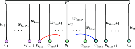
Figure 4: Illustration of a star $T_{V}$ with weights $w_{i}=w(v^{*}v_{i})$ of edge $v^{*}v_{i}\in E(T)$.

We determine a real value to each weight $w_{i}$, where the value may be negative. Recall that we can convert the weights of leaf edges into positive values if necessary without changing the tree in a PCR.

For some $p,q\in[1,n]$ with $p<q$, suppose that weights $w_{i}$ with $p+1\leq i\leq q-1$ and bounds $d_{\min}$ and $d_{\max}$ have been determined so that
  (a) $w_{p+1}\leq w_{p+2}\leq\cdots\leq w_{q-1}$;
  (b) $w_{j}<w_{j+1}$ for $\{v_{j},v_{j+1}\}\not\in M_{G}$ with $j\in[p+1,q-2]$;
  (c) $w_{j}+w_{k}>d_{\min}$ for $(j,k)\in{\tt green}$ with $p+1\leq j<k\leq q-1$,
    $w_{j}+w_{k}<d_{\min}$ for $(j,k)\in{\tt red}$ with $p+1\leq j<k\leq q-1$,
    $w_{h}+w_{j}<d_{\max}$ for $(h,j)\in{\tt green}$ with $p+1\leq h<j\leq q-1$,
    $w_{h}+w_{j}>d_{\max}$ for $(h,j)\in{\tt blue}$ with $p+1\leq h<j\leq q-1$.
Hence for distinct $i,i^{\prime}\in[p+1,q-1]$, it holds $d_{\min}>w_{i}+w_{i^{\prime}}$ if $(i,i^{\prime})\in{\tt red}$; $d_{\min}<w_{i}+w_{i^{\prime}}<d_{\max}$ if $(i,i^{\prime})\in{\tt green}$; and $w_{i}+w_{i^{\prime}}>d_{\max}$ if $(i,i^{\prime})\in{\tt blue}$.

With the next lemma, we start with weights $w_{i}$ with $p+1\leq i\leq q-1$ and bounds $d_{\min}$ and $d_{\max}$ for $p=i_{\tt red}$ and $q=i_{\tt blue}$.

Lemma 11

For a graph $G=(V,E)$ with $n\geq 2$ and an ordering $\sigma=v_{1},v_{2},\ldots,v_{n}$ of $V$, let $c$ be a coloring $c$ of $G$ proper to $(G,\sigma)$. For $p=i_{\tt red}$ and $q=i_{\tt blue}$, there is a set $\{w_{p+1},w_{p+2},\ldots,w_{q-1},d_{\min},d_{\max}\}$ of weights and bounds that satisfies condition (a)-(c).

Proof. Since $(i,j)\in{\tt green}$ for all $i_{\tt red}<i<j<i_{\tt blue}$ by Lemma 10(i), we can easily find required weights $w_{i}$ for all $i$ with $i_{\tt red}<i<i_{\tt blue}$ so that $d_{\min}<w_{i}+w_{i^{\prime}}<d_{\max}$ for all $i,i^{\prime}$ with $i_{\tt red}<i<i^{\prime}<i_{\tt blue}$. For example, such weights $w_{i}$ and bounds $d_{\min}$ and $d_{\max}$ can be obtained as follows.

$d_{\min}:=0$; $w_{i_{\tt red}+1}:=1$;
     for $i=i_{\tt red}+2,i_{\tt red}+3,\ldots,i_{\tt blue}-1$ do
     if $\{v_{i},v_{i+1}\}\in M_{G}$ then
        $w_{i+1}:=w_{i}$
     else
        $w_{i}:=w_{i+1}+1$
     end if;
     $d_{\max}:=2w_{i_{\tt blue}-1}+1$.
∎

Then without changing the determined values to $w_{p+1},w_{p+2},\ldots,w_{q-1}$, we determine $w_{p}$ or $w_{q}$ so that the above condition holds for $(p:=p-1,q)$ or $(p,q:=q+1)$.

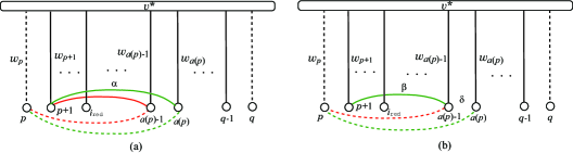
Figure 5: Illustration of a process of determining weight $w_{p}$, where vertex $v_{i}$ is indicated with its index $i$: (a) Case (ii) where $\{v_{p},v_{p+1}\}\not\in M_{G}$ and $a(p+1)=a(p)\leq q-1$; (b) Case (iii) where $\{v_{p},v_{p+1}\}\not\in M_{G}$ and $a(p+1)<a(p)\leq q-1$.

We can determine values to weights $w_{i_{\tt red}},w_{i_{\tt red}-1},\ldots,w_{1}$ in this order as follows.

Lemma 12

For a graph $G=(V,E)$ with $n\geq 2$ and an ordering $\sigma=v_{1},v_{2},\ldots,v_{n}$ of $V$, let $c$ be a coloring $c$ of $G$ proper to $(G,\sigma)$. For $p\leq i_{\tt red}$ and $q\geq i_{\tt blue}$, assume that a set $\{w_{p+1},w_{p+2},\ldots,w_{q-1},$ $d_{\min},d_{\max}\}$ of weights and bounds satisfies conditions (a)-(c). When $p\geq 1$, let weight $w_{p}$ be determined such that

$$w_{p}=\left\{\begin{array}[]{cl}w_{p+1}&\mbox{ if $\{v_{p},v_{p+1}\}\in M_{G}$, }\\ w_{p+1}-\alpha/2&\mbox{ if $\{v_{p},v_{p+1}\}\not\in M_{G}$ and $a(p+1)=a(p)\leq q-1$, }\\ &\mbox{~{}~{}~{} where $\alpha=w_{p+1}+w_{a(p)}-d_{\min}~{}(>0)$, }\\ w_{p+1}-\beta-\delta/2&\mbox{ if $\{v_{p},v_{p+1}\}\not\in M_{G}$ and $a(p+1)<a(p)\leq q-1$, }\\ &\mbox{~{}~{}~{} where $\beta=w_{p+1}+w_{a(p)-1}-d_{\min}~{}(>0)$ and}\\ &\mbox{~{}~{}~{}~{}~{}~{}$\delta=w_{a(p)}-w_{a(p)-1}~{}(>0)$, }\\ \min\{w_{p+1},d_{\min}\!-\!w_{q-1}\}\!-\!1&\mbox{ otherwise, i.e., $\{v_{p},v_{p+1}\}\not\in M_{G}$ and $q\leq a(p)$.}\end{array}\right.$$

Then the set $\{w_{p},w_{p+1},w_{p+2},\ldots,w_{q-1},d_{\min},d_{\max}\}$ of weights and bounds satisfies conditions (a)-(c) for $p^{\prime}=p-1$ and $q$.

Proof. We distinguish the four cases.

(i) $\{v_{p},v_{p+1}\}\in M_{G}$: Since $\{v_{p},v_{p+1}\}\in M_{G}$ and $w_{p}=w_{p+1}$, we see that for each $i\in[p+2,q]$ with $(p,i)\in{\tt green}$ (resp., $(p,i)\in{\tt red}$, ${\tt blue}$) $d_{\min}<w_{p}+w_{i}=w_{p+1}+w_{i}<d_{\max}$ (resp., $w_{p}+w_{i}=w_{p+1}+w_{i}<d_{\min}$ and $w_{p}+w_{i}=w_{p+1}+w_{i}>d_{\max}$). To show that conditions (a)-(c) hold for $(p^{\prime}:=p-1,q)$, it suffices to show that $(p,p+1)\in{\tt red}$ and $w_{p}+w_{p+1}<d_{\min}$. If $p=i_{\tt red}$ then $i_{\tt red}$ would be larger than the current $p$ since $\{v_{p},v_{p+1}\}\in M_{G}$. Hence $p<i_{\tt red}$, which implies that $p+2\leq{\tt red}+1$ and $(p,p+1),(p+1,p+2)\in{\tt red}$. Since ${\tt red}+2\leq i_{blue}$ by Lemma 10(ii), Then $w_{p+1}$ and $w_{p+2}$ have been determined so that $w_{p+1}+w_{p+2}<d_{\min}$ since condition (c) holds. Therefore $w_{p}+w_{p+1}\leq w_{p+1}+w_{p+2}<d_{\min}$ since condition (a) holds.

(ii) $\{v_{p},v_{p+1}\}\not\in M_{G}$ and $a(p+1)=a(p)\leq q-1$: Fig. 5(a) illustrates the case where $\{v_{p},v_{p+1}\}\not\in M_{G}$ and $a(p+1)=a(p)\leq q-1$. Since condition (a) holds and $a(p)\leq q-1$, it holds that $w_{p+1}\leq\cdots\leq w_{a(q)-1}\leq w_{a(q)}\leq w_{q-1}$. Since $a(p+1)=a(p)$, we see that $(p,a(p)-1),(p+1,a(p)-1)\in{\tt red}$ and $(p,a(a)),(p+1,a(p))\in{\tt green}$. Since condition (c) holds for $(p+1,a(p))\in{\tt green}$, we see that $\alpha=w_{p+1}+w_{a(p)}-d_{\min}$ is positive. To show that conditions (a)-(c) hold for $(p^{\prime}:=p-1,q)$, it suffices to show that $w_{p}<w_{p+1}$; $w_{p}+w_{a(p)}>d_{\min}$; and $w_{p}+w_{a(p)-1}<d_{\min}$. Since $\alpha>0$, we have $w_{p}=w_{p+1}-\alpha/2<w_{p+1}$. We next see that $w_{p}+w_{a(p)}=(w_{p+1}-\alpha/2)+w_{a(p)}=d_{\min}+\alpha/2>d_{\min}$, as required. Finally we observe that $w_{p}+w_{a(p)-1}<w_{p+1}+w_{a(p)-1}<d_{\min}$ since condition (c) holds for $(p+1,a(p)-1)\in{\tt red}$.

(iii) $\{v_{p},v_{p+1}\}\not\in M_{G}$ and $a(p+1)<a(p)\leq q-1$: Fig. 5(b) illustrates the case where $\{v_{p},v_{p+1}\}\not\in M_{G}$ and $a(p+1)<a(p)\leq q-1$ As in (ii), we see that $w_{p+1}\leq\cdots\leq w_{a(q)-1}\leq w_{a(q)}\leq w_{q-1}$. Since $a(p+1)<a(p)$, we see that $(p,a(p)-1)\in{\tt red}$ and $(p+1,a(p)-1)\in{\tt green}$. This means that $\{v_{a(p)-1},v_{a(p)}\}\not\in M_{G}$, where $w_{a(q)-1}<w_{a(q)}$ by condition (b) and $\delta=w_{a(p)}-w_{a(p)-1}$ is positive. Since condition (c) holds for $(p+1,a(p)-1)\in{\tt green}$, $\beta=w_{p+1}+w_{a(p)-1}-d_{\min}$ is positive. To show that conditions (a)-(c) hold for $(p^{\prime}:=p-1,q)$, it suffices to show that $w_{p}<w_{p+1}$; $w_{p}+w_{a(p)}>d_{\min}$; and $w_{p}+w_{a(p)-1}<d_{\min}$. Since $\beta,\delta>0$, we have $w_{p}=w_{p+1}-\beta-\delta/2<w_{p+1}$. We next see that $w_{p}+w_{a(p)}=(w_{p+1}-\beta-\delta/2)+(w_{a(p)-1}+\delta)=d_{\min}+\delta/2>d_{\min}$, as required. Finally we observe that $w_{p}+w_{a(p)-1}=(w_{p+1}-\beta-\delta/2)+w_{a(p)-1}=d_{\min}-\delta/2<d_{\min}$, as required.

(iv) $\{v_{p},v_{p+1}\}\not\in M_{G}$ and $q\leq a(p)$: Since $q\leq a(p)$, $(p,i)\in{\tt red}$ for all $i\in[p+1,q-1]$. As in (ii), we see that $w_{p+1}\leq\cdots\leq w_{q-1}$. To show that conditions (a)-(c) hold for $(p^{\prime}:=p-1,q)$, it suffices to show that $w_{p}<w_{p+1}$; and $w_{p}+w_{q-1}<d_{\min}$. Obviously $w_{p}=\min\{w_{p+1},d_{\min}-w_{q-1}\}-1\leq w_{p+1}-1<w_{p+1}$, as required. Finally we observe that $w_{p}+w_{q-1}\leq(d_{\min}-w_{q-1}-1)+w_{q-1}=d_{\min}-1<d_{\min}$, as required. ∎

Analogously with the process of computing weights $w_{i_{\tt red}},w_{i_{\tt red}-1},\ldots,w_{1}$ by Lemma 12, we can choose weights $w_{i_{\tt blue}},w_{i_{\tt blue}+1},\ldots,w_{n}$ in this order as follows.

Lemma 13

For a graph $G=(V,E)$ with $n\geq 2$ and an ordering $\sigma=v_{1},v_{2},\ldots,v_{n}$ of $V$, let $c$ be a coloring $c$ of $G$ proper to $(G,\sigma)$. For $p\leq i_{\tt red}$ and $q\geq i_{\tt blue}$, assume that a set $\{w_{p+1},w_{p+2},\ldots,w_{q-1},$ $d_{\min},d_{\max}\}$ of weights and bounds satisfies conditions (a)-(c). When $q\leq n$, let weight $w_{q}$ be determined such that

$$w_{q}=\left\{\begin{array}[]{cl}w_{q-1}&\mbox{ if $\{v_{q-1},v_{q}\}\in M_{G}$, }\\ w_{q-1}+\alpha/2&\mbox{ if $\{v_{q-1},v_{q}\}\not\in M_{G}$ and $p+1\leq b(q)=b(q-1)$, }\\ &\mbox{~{}~{}~{} where $\alpha=d_{\max}-(w_{b(p)}+w_{q-1})~{}(>0)$, }\\ w_{q-1}+\beta+\delta/2&\mbox{ if $\{v_{q-1},v_{q}\}\not\in M_{G}$ and $p+1\leq b(q)<b(q-1)$, }\\ &\mbox{~{}~{}~{} where $\beta=d_{\max}-(w_{b(p)+1}+w_{q-1})~{}(>0)$ and}\\ &\mbox{~{}~{}~{}~{}~{}~{}$\delta=w_{b(q)+1}-w_{b(q)}~{}(>0)$, }\\ \max\{w_{q-1},d_{\max}\!-\!w_{q-1}\}\!+\!1&\mbox{ otherwise, i.e., $\{v_{q-1},v_{q}\}\not\in M_{G}$ and $b(q)\leq p$.}\end{array}\right.$$

Then the set $\{w_{p+1},w_{p+2},\ldots,w_{q-1},w_{q},d_{\min},d_{\max}\}$ of weights and bounds satisfies conditions (a)-(c) for $p$ and $q^{\prime}:=q+1$.

Proof. Analogously with the proof of Lemma 12. ∎

We are ready to prove Lemma 2. Given a graph $G=(V,E)$ with an gap-free ordering $\sigma=v_{1},v_{2},\ldots,v_{n}$ of $V$, a coloring $c$ of $G$ proper to $(G,\sigma)$ can be obtained in $O(n^{2})$ time by Lemma 3. For the coloring $c$, we first comput $M_{G}$, indices $a(i),b(i)$, $i=1,2,\ldots,n$ and $i_{\tt red}$ and $i_{\tt blue}$ for in $O(n^{3})$ time. Based on these, we can determine weights $w_{i}$ with $i_{\tt red}<i<i_{\tt blue}$ in $O(n)$ time by the method in the proof of Lemma 11. Finally we determine weights $w_{i}$ with $1\leq i\leq i_{\tt red}$ and $i_{\tt blue}\leq i\leq n$ in $O(n)$ time by Lemmas 12 and 13, respectively. This gives a PCR $(T_{V},w,d_{\min},d_{\max})$ of $G$ such that $w_{1}\leq w_{2}\leq\cdots\leq w_{n}$ in $O(n^{3})$ time. This proves Lemma 2.

Appendix 0.F Proof of Lemma 4

Lemma 4 For a graph $G=(V,E)$ with a gap-free ordering $\sigma=v_{1},v_{2},\ldots,v_{n}$ of $V$ and a coloring $c$ proper to $\sigma$, let $V_{1}=\{v_{i}\mid 1\leq i\leq i_{\tt red}\}$, $V_{2}=\{v_{i}\mid i_{\tt blue}\leq i\leq n\}$, and $V^{*}=\{v_{i}\mid i_{\tt red}-1\leq i\leq i_{\tt blue}+1\}$. Then

1. If two edges $v_{i}v_{j}$ and $v_{i^{\prime}}v_{j^{\prime}}$ with $i<j$ and $i^{\prime}<j^{\prime}$ cross $($i.e., $i<i^{\prime}<j<j^{\prime}$ or $i^{\prime}<i<j^{\prime}<j)$, then they belong to the same component of $G$;

2. It holds $i_{\tt red}+1\leq i_{\tt blue}-1$. The graph $G[V^{*}]$ is a complete graph, and $G-V^{*}$ is a bipartite graph between vertex sets $V_{1}$ and $V_{2}$; and

3. Every two vertices $v_{i},v_{j}\in V_{1}\cap N_{G}(V^{*})$ with $i<j$ satisfy $v_{i_{\tt blue}-1}\in N_{G}(v_{i})\cap V^{*}\subseteq N_{G}(v_{j})\cap V^{*}\subseteq V^{*}\setminus\{v_{i_{\tt red}+1}\}$; and
   Every two vertices $v_{i},v_{j}\in V_{2}\cap N_{G}(V^{*})$ with $i<j$ satisfy $v_{i_{\tt red}+1}\in N_{G}(v_{j})\cap V^{*}\subseteq N_{G}(v_{i})\cap V^{*}\subseteq V^{*}\setminus\{v_{i_{\tt blue}-1}\}$.

Proof. (i) Let edges $e=v_{i}v_{j},e^{\prime}=v_{i^{\prime}}v_{j^{\prime}}\in E$ cross, where $i<i^{\prime}<j<j^{\prime}$. If $e$ and $e^{\prime}$ belong to different components of $G$, then $\{v_{i^{\prime}},v_{j}\}$ would a gap with respect to edges $e$ and $e^{\prime}$.

(ii) Immediate from Lemma 10(ii).

(iii) We show that every two vertices $v_{i},v_{j}\in V_{1}\cap N_{G}(V^{*})$ with $i<j$ satisfy $v_{i_{\tt blue}-1}\in N_{G}(v_{i})\cap V^{*}\subseteq N_{G}(v_{j})\cap V^{*}\subseteq V^{*}\setminus\{v_{i_{\tt red}+1}\}$ (the other case can be treated symmetrically). For this, it suffices to show that, for any vertex $v_{i}\in V_{1}$ with $N_{G}(v_{i})\cap V^{*}\neq\emptyset$,
   (a) it holds $v_{i_{\tt blue}-1}\in N_{G}(v_{i})$; and
   (b) for any vertex $v\in N_{G}(v_{j})\cap V^{*}$ with $v_{j}\in V_{1}$ and $i<j$,
      it holds that $v\in N_{G}(v_{i})$.
In (a), otherwise $\{v_{i},v_{i_{\tt blue}-1}\}$ would be a gap with respect to edges $v_{i}v$ and $vv_{i_{\tt blue}-1}$ for any vertex $v\in N_{G}(v_{i})\cap V^{*}$. In (b), otherwise $\{v_{j},v\}$ would be a gap with respect to edges $v_{i}v$ and $v_{j}v_{i_{\tt blue}-1}$. ∎

Appendix 0.G Proof of Lemma 6

Lemma 6 Let $G=(V_{1},V_{2},E)$ be a connected bipartite graph with $|E|\geq 1$. Then family $\mathcal{S}_{i}$ is separator-free for each $i=1,2$, and $G$ has a gap-free ordering of $V$ if and only if for each $i=1,2$, family $\mathcal{S}_{i}$ admits a contiguous ordering $\sigma_{i}$ of $V_{i}$. For any contiguous ordering $\sigma_{i}$ of $V_{i}$, $i=1,2$, one of orderings $(\sigma_{1},\sigma_{2})$ and $(\sigma_{1},\overline{\sigma_{2}})$ of $V$ is a gap-free ordering to $G$.

Proof. Since $G$ is connected, we see that, for each $i=1,2$, the family $\mathcal{S}_{i}$ is separation-free.

The only if part: Let $v_{1},v_{2},\ldots,v_{k},v_{k+1},\ldots,v_{n}$ be a gap-free ordering of $V$ to $G$, where $V_{1}=\{v_{1},v_{2},\ldots,v_{k}\}$ and $V_{2}=\{v_{k+1},\ldots,v_{n}\}$. Since there is no gap, for each vertex $v\in V_{2}$, the neighbors in $N_{G}(v)$ appear consecutively as a subsequence of $v_{1},v_{2},\ldots,v_{k}$. Also for any two vertices $u,v\in V_{2}$ such that $N_{G}(u)$ is a proper subset of $N_{G}(v)$, the subsequence $v_{i},v_{i+1},\ldots,v_{j}$ for $N_{G}(u)$ must contain the first vertex or the last vertex in the subsequence $v_{h},v_{h+1},\ldots,v_{p}$ for $N_{G}(v)$. This is because otherwise $v_{h},v_{p}\not\in N_{G}(u)$ would imply that $\{u,v_{h}\}$ (or $\{u,v_{p}\}$) is a gap with respect to edges $e_{1}=uv_{i}$ and $e_{1}=vv_{h}$ (or $e_{1}=uv_{j}$ and $e_{1}=vv_{p}$). Therefore $v_{1},v_{2},\ldots,v_{k}$ is a contiguous ordering of $V_{1}$ to $\mathcal{S}_{1}$. Analogously with $V_{2}$ and $\mathcal{S}_{2}$.

The if part: Assume that for each $i=1,2$, the family $\mathcal{S}_{i}$ has a contiguous ordering $\sigma_{i}$ of $V_{i}$. Note that any set $X\in\mathcal{X}_{\mathcal{S}_{i}}$, $i=1,2$ is either contained in $N_{G}(v)$ or disjoint with $N_{G}(v)$ for each vertex $v\in V_{j}$, $j\neq i$. By Theorem 3.2 applied to $\mathcal{S}_{i}$, the vertices in each maximal set $X\in\mathcal{X}_{\mathcal{S}_{i}}$ appear consecutively in any contiguous ordering of $V(\mathcal{S}_{i})$. Also a contiguous ordering of $V(\mathcal{S}_{i})$ is unique up to reversal and choice of an ordering of each set $X\in\mathcal{X}_{\mathcal{S}_{i}}$. This means that an ordering $\sigma=(\sigma_{1},\sigma_{2})$ or $(\sigma_{1},\overline{\sigma_{2}})$ of $V$ is gap-free if and only if any ordering obtained from $\sigma$ by changing an ordering of vertices in each set $X\in\mathcal{X}_{\mathcal{S}_{1}}\cup\mathcal{X}_{\mathcal{S}_{2}}$. Therefore, to see if $G$ admits a gap-free ordering of $V$, we only need to check if at least one of $(\sigma_{1},\sigma_{2})$ and $(\sigma_{1},\overline{\sigma_{2}})$ is gap-free in $G$. ∎

Appendix 0.H Proof of Lemma 7

Lemma 7 For a connected non-bipartite graph $G=(V,E)$ with $V^{\tt t}\neq\emptyset$, and let $v^{*}_{1},v^{*}_{2}$ be two adjacent vertices in $V^{\tt t}$. Let $V^{*}=\{v^{*}_{1},v^{*}_{2}\}\cup(N_{G}(v^{*}_{1})\cap N_{G}(v^{*}_{2}))$, $V^{\prime}_{1}=N_{G}(v^{*}_{2})\setminus V^{*}$, and $V^{\prime}_{2}=N_{G}(v^{*}_{1})\setminus V^{*}$. Assume that $G$ has a gap-free ordering $\sigma$ of $V$ and a proper coloring $c$ to $\sigma$ such that $v^{*}_{1}=v_{i_{\tt red}+1}$, $v^{*}_{2}=v_{i_{\tt blue}-1}$. Then:

1. A maximal clique $K_{v^{*}_{1},v^{*}_{2}}$ of $G$ that contains edge $v^{*}_{1},v^{*}_{2}$ is uniquely given as $G[V^{*}]$. The graph $G[V^{*}]$ is the core of the ordering $\sigma$, and $G-V^{*}$ is a bipartite graph $(V_{1},V_{2},E^{\prime})$; and

2. Let $\mathcal{S}_{i}$ be the family $\{N_{G}(v)\mid v\in V_{j}\}$ for $\{i,j\}=\{1,2\}$, and $\mathcal{S}=\mathcal{S}_{1}\cup\mathcal{S}_{2}\cup\{V^{*}\}$. Then $\mathcal{S}$ is a separator-free family that admits a contiguous ordering $\sigma$ of $V$, and any contiguous ordering $\sigma$ of $V$ is a gap-free ordering to $G$.

Proof. (i) By Lemma 5(ii), we see that $\{v_{i}\mid i_{\tt red}+1<i<i_{\tt blue}-1\}\subseteq N_{G}(v_{i_{\tt red}+1})\cap N_{G}(v_{i_{\tt blue}-1})$. On the other hand, by Lemma 5(ii), vertex $v_{i_{\tt red}+1}$ (resp., $v_{i_{\tt blue}-1}$) is not adjacent to any vertex in $V_{2}$ (resp., $V_{1}$) in $G$. Hence $\{v_{i_{\tt red}+1},v_{i_{\tt blue}-1}\}\cup(N_{G}(v_{i_{\tt red}+1})\cap N_{G}(v_{i_{\tt blue}-1}))$ induces uniquely a maximal clique that contains $v_{i_{\tt red}+1}$ and $v_{i_{\tt blue}-1}$. Hence the clique is the core of the gap-free ordering of $V$. By Lemma 4(ii), $G-V^{*}$ is a bipartite graph $(V_{1},V_{2},E^{\prime})$.

(ii) Since $G$ is connected, we see that $\mathcal{S}_{i}$ is separation-free. First we prove that $\mathcal{S}$ admits a contiguous ordering of $V$. Any set $S\in\mathcal{S}$ with $S\cap V^{*}\neq\emptyset$ satisfies one of the following:
  - $v_{i_{\tt red}+1}\not\in S$ and $v_{i_{\tt blue}-1}\in S\in\mathcal{S}_{2}$;
  - $v_{i_{\tt blue}-1}\not\in S$ and $v_{i_{\tt red}+1}\in S\in\mathcal{S}_{1}$; and
  - $v_{i_{\tt red}+1},v_{i_{\tt blue}-1}\in S=V^{*}$.
This means that any two sets $S,S^{\prime}\in\mathcal{S}$ with $S\subseteq S^{\prime}$ belong to the same family $\mathcal{S}_{i}$. Hence any gap-free ordering $\sigma$ of $V$ to $G$ is a contiguous ordering of $V$ to $\mathcal{S}$, as discussed in the proof of the only if part of Lemma 6.

Next we prove that any contiguous ordering $\sigma$ of $V$ to $\mathcal{S}$ is a gap-free ordering of $V$ in $G$. Since $G$ is connected, each $\mathcal{S}_{i}$ is separator-free in $V(\mathcal{S}_{i})$. We see that $\mathcal{S}=\mathcal{S}_{1}\cup\mathcal{S}_{2}\cup\{V^{*}\}$ is separator-free in $V$ even if $V(\mathcal{S}_{1})\cap V(\mathcal{S}_{2})\neq\emptyset$. Note that any set $X\in\mathcal{X}_{\mathcal{S}}$ is either contained in $N_{G}(v)$ or disjoint with $N_{G}(v)$ for each vertex $v\in V_{j}$, $j\neq i$. By Theorem 3.2 applied to $\mathcal{S}$, the vertices in each maximal set $X\in\mathcal{X}_{\mathcal{S}}$ appear consecutively in any contiguous ordering of $V(\mathcal{S})$. Also a contiguous ordering of $V(\mathcal{S})$ is unique up to reversal and choice of an ordering of each set $X\in\mathcal{X}_{\mathcal{S}}$. This means that an ordering $\sigma$ of $V$ is gap-free if and only if any ordering obtained from $\sigma$ by changing an ordering of vertices in each set $X\in\mathcal{X}_{\mathcal{S}}$. Therefore any contiguous ordering $\sigma$ of $V$ to $\mathcal{S}$ is a gap-free ordering of $V$ in $G$. ∎

References

- [1] S. Booth and S. Lueker, Testing for the consecutive ones property, interval graphs, and graph planarity using PQ-tree algorithms, J. Comput. Syst. Sci., 13 (1976) 335–379
- [2] A. Brandstädt, On leaf powers, Technical report, University of Rostock, 2010.
- [3] T. Calamoneri, D. Frascaria, and B. Sinaimeri, All graphs with at most seven vertices are pairwise compatibility graphs, The Computer Journal, 56(7) (2013) 882–886
- [4] T. Calamoneri, A. Frangioni, and B. Sinaimeri, Pairwise compatibility graphs of caterpillars, The Computer Journal, 57(11) (2014) 1616–1623
- [5] T. Calamoneri and R. Petreschi, On pairwise compatibility graphs having Dilworth number two, Theoret. Comput. Sci., 524 (2014) 34–40
- [6] T. Calamoneri, R. Petreschi, and B. Sinaimeri, On the pairwise compatibility property of some superclasses of threshold graphs, Discrete Math. Algorithms Appl., 5(2) (2013), article 360002
- [7] T. Calamoneri and B. Sinaimeri, Pairwise compatibility graphs: A survey, SIAM Review 58(3)(2016) 445–460
- [8] Z.-Z. Chen, T. Jiang, and G. Lin, Computing phylogenetic roots with bounded degrees and errors, SIAM J. Comput., 32 (2003) 864–879
- [9] S. Durocher, D. Mondal, and Md. S. Rahman, On graphs that are not PCGs, Theoret. Comput. Sci., 571 (2015) 78–87
- [10] J. Felsenstein, Cases in which parsimony or compatibility methods will be positively misleading, Systematic Zoology, 27 (1978) 401–410
- [11] Md. I. Hossain, S. A. Salma, Md. S. Rahman, and D. Mondal, A necessary condition and a sufficient condition for pairwise compatibility graphs, J. Graph Algorithms Appl. 21(3) (2017) 341–352
- [12] P. E. Kearney, J. I. Munro, and D. Phillips, Efficient generation of uniform samples from phylogenetic trees, in Algorithms in Bioinformatics, G. Benson and R. Page, eds., LNCS 2812, Springer, Berlin, Heidelberg, 2003, 177–189
- [13] G. Lin, P. E. Kearney, and T. Jiang, Phylogenetic k-root and Steiner k-root, in Algorithms and Computation, G. Goos, J. Hartmanis, J. van Leeuwen, D. T. Lee, and S.-H. Teng, eds., LNCS 1969, Springer, Berlin, Heidelberg, 2000, 539–551
- [14] S. Mehnaz and Md. S. Rahman, Pairwise compatibility graphs revisited, in Proceedings of the 2013 International Conference on Informatics, Electronics Vision (ICIEV), 2013, 1–6
- [15] N. Nishimura, P. Ragde, and D. M. Thilikos, On graph powers for leaf-labeled trees, J. Algorithms, 42 (2002) 69–108
- [16] S. A. Salma, Md. S. Rahman, and Md. I. Hossain, Triangle-free outerplanar 3-graphs are pairwise compatibility graphs, J. Graph Algorithms Appl., 17 (2013) 81–102
- [17] M. Xiao and H. Nagamochi, Some reduction operations to pairwise compatibility graphs, Technical report 2017-003, December 1, 2017, http://www-or.amp.i.kyoto-u.ac.jp/members/nag/Technicalreport/TR2017-003.pdf
- [18] M. N. Yanhaona, Md. S. Bayzid, and Md. S. Rahman, Discovering pairwise compatibility graphs. Discrete Math., Alg. and Appl. 2(4)(2010) 607–624
- [19] M. N. Yanhaona, K. S. M. T. Hossain, and Md. S. Rahman, Pairwise compatibility graphs, in: WALCOM 2008, 2008, 222–233