Invariant measures of disagreement with stochastic dominance.

Abstract

An essential feature of stochastic order is its invariance against increasing maps. In this paper, we analyze a family of invariant indices of disagreement with respect to stochastic dominance. The indices in this family admit the representation $\theta(F,G)=P(X>Y)$, where $(X,Y)$ is a random vector with marginal distribution functions $F$ and $G$. This includes the case of independent marginals, but also other interesting indices related to a contamination model or to a joint quantile representation. For some choices of $\theta$ the condition $\theta(F,G)=0$ is equivalent to stochastic dominance of $G$ over $F$. We show that the index associated to the contamination model achieves the minimal value within this family. The plug-in sample-based versions of these indices lead to the Mann-Whitney, the one-sided Kolmogorov-Smirnov, and the Galton statistics. For some of the most interesting indices this fact provides sufficient theoretical support for asymptotic inference. However, this is not the case for Galton’s statistic, for which we provide additional theory for its resampling behaviour. We stress on the complementary roles of some of these indices, which beyond measuring disagreement with respect to stochastic order allow to describe the maximum possible difference in status of a value $x\in\mbox{$\mathbb{R}$}$ under $F$ or $G$. We apply these indices to some real data sets.

Keywords: relaxed stochastic dominance, asymptotics, inferential procedures, $P(X>Y)$-representation, Galton’s rank statistic.

1 Introduction

Comparison is a customary task in any type of research or activity. However, although being almost instinctive when it involves measurements on just two individuals, it is far from being obvious when it refers to two populations; for instance, if we are interested in comparing a feature over two given populations, except in the trivial case where all the members of one population exhibit lower values than all of the other population, the task admits very different points of view. Often it is approached through the comparison of the means or some other summary value (median, Gini index,…), but the real meaning of such comparison is not so obvious and, sometimes, it is even wrongly interpreted by the practitioners. This situation was addressed in Álvarez-Esteban et al. (2017), emphasizing on location-scale models, defending the stochastic order as the natural gold standard behind two-sample comparison problems. To pursue in that direction, here we will come back to the very principles of comparison, by considering the real meaning of stochastic order between probability distributions and analyzing some natural relaxations intended to measure the disagreement level with such stochastic order.

Let us begin by considering a simple generic statement like “people is richer today than four years ago”. If we understand that expression in terms of per capita income, its precise meaning would be that if we compute the mean income of a (randomly) chosen group of individuals today and that of another group four years ago, both large enough, almost certainly the per capita income of the former would be greater than the second. Nonetheless, as it is stressed, for instance, in Álvarez-Esteban et al. (2017), such a comparison is compatible with very different shapes of the parent distributions, and could lead to a false picture, highly unsuitable e.g. when a skewed, very heavy tailed distribution is involved. An order between populations or distributions should indicate a comprehensive relation between them, improving those based on making comparisons through single indices or features of the distributions.

To simplify the initial exposition and produce sensible pictures, let us begin by considering the comparison of the incomes of two equal-sized populations ($n=20$) of individuals today and four years ago, represented in Figure 1 through black and white bars. In the left-graphic there, we can observe that there is some trend towards higher values of the black bars on the white bars in spite of there are white bars that are larger than some black ones. To check if the black population stochastically dominates the white one, the right-graphic shows the same bars but now matching the smallest black bar with the smallest white, the second with the second, …, and so on. By comparing the ordered elements with equal rank in their respective populations, we see that any black bar is larger than its paired white one. This is a relationship we recognise as stochastic dominance of the incomes of the first population over the second one: The comparison between the individuals with same rank is just the comparison between quantile functions given in (1).

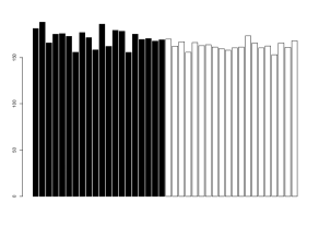
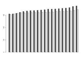
Figure 1: Barplots of the incomes of a sample of 20 individuals today (black bars) and those of another sample, with the same size, four years ago (white bars). The right-picture pairs the individual incomes corresponding to the ordered values in each sample.

Let be given two probability distributions on the real line, $\mathbb{R}$, defined through their distribution functions (d.f.’s) $F$ and $G$. Denoting by $F^{-1}$ to the quantile function of $F$ (that we recall is defined by $F^{-1}(t):=\inf\{x:\ t\leq F(x)\}$, for $t\in(0,1)$), we say that $F$ is stochastically dominated by $G$, denoted $F\leq_{st}G$, if

$$F^{-1}(t)\leq G^{-1}(t)\mbox{ for every }t\in(0,1).$$ (1)

This definition is equivalent to the usual definition of stochastic dominance, namely:

$$F\leq_{st}G\mbox{ \it whenever }F(x)\geq G(x)\mbox{ \it for every }x\in\mbox{$\mathbb{R}$},$$ (2)

while, as noted in Lehmann (1955), (1) is more intuitive.

Note that for a value, $x$, obtained from the distribution $F$ (resp. $G$), the value $F(x)$ (resp. $G(x)$) can be considered as the “status” of that value in the first (resp. second) population. In this sense, the meaning of (2) is that the status of any individual value would be higher when considered in the first population than when considered in the second. On the other hand, recall that when defined on the unit interval $(0,1)$ equipped with the Lebesgue measure, $\ell$, the quantile function $F^{-1}$ is a random variable (r.v.) with d.f. $F$. This fact and (1) lead to a further equivalent and appealing characterization of stochastic dominance:

$$\begin{array}[]{c}F\leq_{st}G\ \mbox{\it if and only if there exist r.v.'s }X,Y\mbox{\it defined on some probability}\\[5.69054pt] \mbox{ \it space }(\Omega,\sigma,P),\mbox{ \it with d.f.'s }F,G,\mbox{\it such that }{P(X\leq Y)=1.}\end{array}$$ (3)

Remark 1.1

This representation, makes it clear that the stochastic dominance is invariant through increasing functions because if $X,Y$ are two r.v.’s whose respective d.f.’s satisfy $F\leq_{st}G$, and $\psi:\mbox{$\mathbb{R}$}\to\mbox{$\mathbb{R}$}$ is increasing, then the d.f. of $\psi(Y)$ also stochastically dominates this one of $\psi(X)$. $\bullet$

Through representation (3) in terms of pairs of r.v.’s $X,Y$, we are fixing a joint distribution with marginals $F$ and $G$, which makes possible to design a sampling procedure able to produce simultaneous samples from both distributions. Therefore, after (3), the meaning of the stochastic dominance $F\leq_{st}G$ is that we can design a joint simulation procedure for $F$ and $G$ such that for every realization, the value from $F$ is lower or equal than that obtained from $G$. The quantile functions give a canonical representation that allows to characterize the stochastic dominance, but (3) opens the possibility to other representations of stochastic dominance in terms of almost sure dominance.

While it is hard to argue against the interest of the stochastic order dominance, it is often observed that such a relation is too strong as to be guaranteed in practice. As an example of this kind of claim, Arcones et al. (2002) notes that the dominance (2) may well hold over an important part of the range but it may fail over another small part of the range, or may simply be unknown or unknowable over the entire range (a fact also implicit in Leshno and Levy (2002) although presented in terms of utility functions). Even worse, from an inferential point of view, as noted in Berger (1988), it is not possible to statistically guarantee the existence of stochastic dominance: If we want to conclude that stochastic order holds we should gather statistical evidence to reject the null in the testing problem of $H_{0}:F\nleq_{st}G\mbox{ vs }H_{a}:F\leq_{st}G.$ But, on the basis of samples obtained from the corresponding distributions, the test that rejects the null tossing a coin with probability of heads equal to $\alpha$, paying no attention to the data, is the uniformly most powerful at level $\alpha$.

Following ideas that go back to Hodges and Lehmann (1954), these facts invite to consider relaxed versions of stochastic order for which feasible statistical tests can be designed. This is often carried out say through a suitable distance, say through contamination neighbourhoods or through combinations of both methods. In any case the goal is to enlarge the null by including “similar” distributions leading to reject it just if there are “relevant changes” on the original hypothesis (Rudas et al. (1994), Munk and Czado (1998), Liu and Lindsay (2009), Álvarez-Esteban et al. (2012), or recently Dette and Wied (2016) and Dette and Wu (2018) share this point of view).

We can mention several interesting examples of relaxations of stochastic order. The ‘stochastic precedence’ relation, introduced in Arcones et al. (2002), is related to the probability of obtaining greater values under $F$ than under $G$ when independently sampled (see Subsection 2.2). More easily interpretable are some indices intended to measure the extent to which stochastic dominance is violated. In this line, we are aware of the approach for “almost stochastic dominance”, introduced in Leshno and Levy (2002), which is based on measuring the relative contribution of $|F-G|$ on the set $(F<G)$, where (2) is not satisfied, to the $L_{1}$ distance between $F$ and $G$. Yet, Álvarez-Esteban et al. (2016) proposed another index based on the contamination model (see Subsection 2.3).

Our objective is to analyse indices to evaluate the extent to which a d.f. $G$ stochastically dominates another $F$, having in mind that the invariance of the stochastic order with respect to increasing maps in the sense of Remark 1.1 makes it desirable that any proposed index should share this invariance. This goal, makes natural considering pairs of r.v.’s $(X,Y)$ with marginal d.f.’s $F$ and $G$ and take indices defined as $P(X>Y)$, although this index will strongly depend of the joint law of $(X,Y)$, relating the marginal laws $F$ and $G$.

An index in this line appears in Álvarez-Esteban et al. (2017), measuring the size of the set where the associated quantile functions do not satisfy the point-wise order (1). For a better understanding of our general approach, we will present that index by resorting to the comparison of finite populations, handling two new populations similar to those considered in Figure 1. The barplot on the left of Figure 2 has been produced in the same way as in the right one in Figure 1. In these populations most black bars are larger than the corresponding white ones, but it is not the case for the third and fourth pairs, thus, in these populations, according to (1), there is no stochastic dominance of the inputs of the second population over those in the earlier. However we can give a precise measure of the extent at which the dominance is not satisfied: 2/20. More precisely, for 90% of the individuals associated to white bars, their status according to their income level would be worse if they were considered in the population associated to black bars. The worsening of status of a person would mean that he/she would be considered less rich today than it was four years ago if its income does not vary. We notice that this index is just the same used by Galton to answer a query by Darwin in 1876 (see Subsection 2.1).

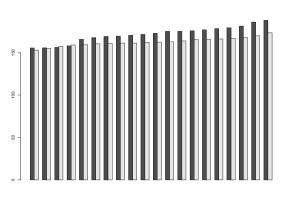
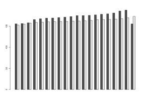
Figure 2: Left: Barplot obtained pairing the 20 individuals with equal rank in their respective sample. Right: White bars concide with the ones in the left; black bars are moved one position to the left, excepting the first one that is moved to the last position.

Let us stress that ranking the individuals of both populations results on an easier comparison of the populations, based on just comparing the pairs formed by the elements sharing identical rank, which is a particular application of the philosophy inspirating (3). However, in principle, any joint representation $(X,Y)$ of the two populations, defined on a suitable probability space, would give a sense to a question like “how large is $P(X>Y)$?”; thus we could choose a different coupling strategy for comparison. In fact, if we couple the highest white bar with the smallest black one and pair the remaining ones by order (see the right graph in Figure 2), we could measure the disagreement with the stochastic order as 1/20. Moreover, it is easy to see that there is no coupling improving this index. To our best knowledge, the consideration of the coupling most compatible with pointwise order has not been addressed until now in the literature. This is adressed in Section 2.3.

As we show in this paper, several proposals of relaxed versions of stochastic order can be analyzed through this common framework that takes advantage of basic coupling ideas. In particular we will solve the already mentioned problem of obtaining a coupling $(X,Y)$ whose associated index $P(X>Y)$ takes the minimum possible value. Unexpectedly, this problem is related to the contamination index introduced in Álvarez-Esteban et al. (2016), which also plays a keynote role in this approach (see Section 2.4).

We notice at this point that among the already mentioned indices, only the index associated to the Leshno and Levy (2002) approach, defined by

$$\epsilon(F,G):=\frac{\int(G(x)-F(x))^{+}dx}{\int|G(x)-F(x)|dx},$$ (4)

fails to satisfy the invariance with respect to increasing maps (it is only invariant with respect to increasing linear functions). In particular, this shows that $\epsilon(F,G)$ does not admit a $P(X>Y)$-representation.

We show that our relaxed versions of stochastic order can be assessed through valid inferential procedures using the corresponding plug-in estimators of the indices. That is, the indices computed on the basis of sample distribution functions. Let us also notice that the statistical analysis of $P(X>Y)$ began in Birnbaum (1965), and under the suggestive title of Stress-Strength Model is widely recognized by its multiple applications (see Kotz et al. (2003) for a general account). We will see that the considered indices involve well known statistics: the Mann-Whitney version of the Wilcoxon statistic (for the $\rho$-index), the one-sided Kolmogorov-Smirnov statistic (for the $\pi$-index), and Galton’s rank order statistic (for the $\gamma$-index). While the available literature on the asymptotics for the first and second statistics suffices for their use in this setting, for the Galton statistic just recent findings on its complex behaviour allow to handle it with some generality. However, the disappointing fact that the ordinary bootstrap does not work for Galton’s statistic has forced us to develop some new additional theory (included in the Appendix) concerning resampling techniques for this statistic leading to Theorem 3.3.

Obviously, the considered indices give different values to the disagreement with the stochastic dominance of $G$ over $F$. Firstly, the $\rho$ index (see the definition in (6)) can be as close as desired to a half in cases in which $G\geq_{st}F$ and equal to a half in cases in which $G$ is very far to dominate $F$. However, this index is useful if, for instance, we are interested into compare two treatments to be applied to independent populations.

Secondly, the $\gamma$ and $\pi$ indices (definitions in (5) and (8)) are more precise evaluations of the lack of stochastic dominance because, for instance, $\gamma(F,G)=0$ (resp. $\pi(F,G)=0$) is equivalent to $G\geq_{st}F$. Moreover, the discussion in Remark 2.8, allows to conclude that $\gamma$ and $\pi$ enjoy some kind of complementarity. First, $\gamma$ gives a more accurate idea than $\pi$ on how far is $G$ to stochastically dominate $F$: for instance, $\gamma(F,G)=1$ is equivalent to $G\geq_{st}F$. However, it is not difficult to imagine situations in which $G\geq_{st}F$, while $F$ and $G$ are as close as desired. Then $\pi$ (through its characterization in (10)) helps to measure this closeness: if we consider the value $F(x)$ (resp. $G(x)$) as the “status” of the value $x\in\mbox{$\mathbb{R}$}$ inside a population with d.f. $F$ (resp. $G$) then $\pi$ gives the biggest possible difference in those status for any value $x$. Obviously, this difference will be small in those cases in which $F$ and $G$ are similar irrespective of the value of $\gamma$.

The paper is structured in the following way: First, through the Subsections 2.1, 2.2 and 2.3 we give a quick overview of the already mentioned indices. Then, in Subsection 2.4, we introduce the framework to analyze these indices from a common perspective. Section 3 includes the pertinent comments and theory for the statistical use of the indices. We also provide, in Section 4, the analysis of several real data sets showing the performance of these indices in applied settings. The mentioned Appendix also contains supplementary information on these data sets.

Let us include now some words on notation. Through the paper $\mathcal{L}(X)$ will denote the law of the random vector or variable $X$, and ${\mathcal{L}}(X/A)$ and ${\mathcal{L}}(X/Z)$ the conditional laws of $X$ given the event $A$ and the, possibly infinite-dimensional, random vector $Z$. We will consider a generic probability space $(\Omega,\sigma,P)$, where the involved random objects are defined and verify the current assumptions ad hoc. $\ell$ will denote the Lebesgue measure on the unit interval $(0,1)$. Convergences in the almost surely or in law (or weak) senses will respectively denoted by $\rightarrow_{\mbox{a.s.}}$ and $\rightarrow_{w}$. Given a real value, $x$, we will write $x^{+}$ for $\max(x,0)$.

The symbols $X,Y$, with or without sub/super-indices, will denote real r.v.’s with respective d.f.’s $F$ and $G$. In particular, $\{X_{n}\}$ and $\{Y_{m}\}$ are independent random samples taken respectively from $F$ and $G$. The empirical d.f.’s associated to random samples with sizes $n$ and $m$ are respectively denoted $F_{n}$ and $G_{m}$.

Finally, we notice that throughout the term increasing means strictly increasing and that sometimes we use the word dominance as an abbreviation for stochastic dominance.

2 Measuring departures from stochastic order

In this section we discuss some indices to measure the departures from the stochastic order. In order to give an intuitive idea of the ways that the different approaches focus to measure the lack of stochastic dominance, we consider the case in which two populations with the same number of individuals are involved. More precisely, we will consider the following example.

Example 2.1

Assume that ${\mathcal{X}}=\{x_{1},\dots,x_{n}\}$ and ${\mathcal{Y}}=\{y_{1},\dots,y_{n}\}$ are the heights of some individuals belonging to different populations.

To analize a possible dominance of the height of population ${\mathcal{Y}}$ over that of ${\mathcal{X}}$, we can reorder the individuals of both populations according to their heights leading to ${\mathcal{X}}=\{x^{*}_{1}\leq\dots\leq x^{*}_{n}\}$ and ${\mathcal{Y}}=\{y^{*}_{1}\leq\dots\leq y^{*}_{n}\}$. In this way, stochastic dominance would be equivalent to $x^{*}_{i}\leq y^{*}_{i}$ for every $i=1,\dots,n$, corresponding just to the comparison between the individuals with identical height rank in each population.

Additionally, to illustrate the behaviour of the different indices, we include comparisons between some fixed normal distributions that play a kind of reference role. To get a quick visual perspective of the relation between some of these indices to measure stochastic dominance, we refer to the contour plots relating normal distributions in Álvarez-Esteban et al. (2017).

Example 2.1 (Cont.) The index $\epsilon$ defined in (4) depends not only on how many pairs $(x_{i}^{*},y_{i}^{*})$ do verify $x^{*}_{i}>y^{*}_{i}$, but, according to (4), it also does on the quantities ${x^{*}_{i}-y^{*}_{i}},$ because, its value in this case is $\sum_{i=1}^{n}({x^{*}_{i}-y^{*}_{i}})^{+}/\sum_{i=1}^{n}|{x^{*}_{i}-y^{*}_{i}}|.$

2.1 The quantile approach

The quantile representation $X^{*}=F^{-1}$ and $Y^{*}=G^{-1}$ defined on $(0,1)$ with the uniform distribution translates the arguably more abstract concept of stochastic order to the more familiar pointwise ordering between $X^{*}$ and $Y^{*}$. We note that from the quantile characterization it follows easily that if $X,Y$ have normal distributions $N(\mu_{1},\sigma_{1}^{2})$ and $N(\mu_{2},\sigma_{2}^{2})$, respectively, $X\leq_{st}Y$ will hold if and only if $\sigma_{1}=\sigma_{2}$ and $\mu_{1}\leq\mu_{2}$. Therefore, if e.g. $\sigma_{1}=10,\sigma_{2}=20,$ the stochastic order relation would be impossible, although, for example, if $\mu_{1}=0,\mu_{2}=16$, the subset of $(0,1)$ where (1) fails is the interval $(0,0.055)$. In other words, a mechanism generating data using $X^{*}$ and $Y^{*}$ would only produce lower values for $Y^{*}$ than for $X^{*}$ in around 5% of cases, while for $\mu_{2}=5$ it would be about 30%. This observation led to define in Álvarez-Esteban et al. (2017) the following index to measure the disagreement level with the stochastic order between distributions

$$\gamma(F,G):=\ell(t:F^{-1}(t)>G^{-1}(t)).$$ (5)

Example 2.1 (Cont.) If there exist $m$ pairs $(x_{i}^{*},y_{i}^{*})$ in Example 2.1, such that $x^{*}_{i}>y^{*}_{i}$, then the $\gamma$-index approach would report the value $m/n$ as the measure of lack of dominance.

The index $\gamma$ allows to quantify the importance of the set where a (restricted) stochastic dominance holds, a concept already considered in Berger (1988), Lehmann and Rojo (1992) and Davidson and Duclos (2013). We also notice that the theory developed in Álvarez-Esteban et al. (2017) was adapted in Zhuang et al. (2019) under the additional assumption of an exponential density ratio model and using semiparametric estimates of the quantile functions. Notice that invariance makes no sense under this semiparametric approach because the exponential density ratio model is lost under most of increasing transformations.

An statement like $\gamma(F,G)\leq\gamma_{0}$, for some fixed (small) $\gamma_{0}$ would give a quantified approach to an approximate stochastic order. Let us also note the trivial facts that $\gamma(F,G)=0$ if and only if $F\leq_{st}G$ and that, for any pair of continuous d.f.’s which coincide, at most on a denumerable set of points, the relation $\gamma(F,G)+\gamma(G,F)=1$ holds.

In the two-sample setting this index would be the value of Galton statistic. This statistic has been considered in the literature just to reject, for small enough values of $\gamma(F,G)$, the null hypothesis that the treatment is without effect ($F=G$), in favour of the alternative that the treatment tends to increase the measurements ($F\lneq_{st}G$).

As explained in Example III.1 b) in Feller (1968) or in Hodges (1955), Galton used this procedure to answer in the positive sense to a query of Charles Darwin on a data set composed by two samples of size 15 for which only two times the order was reversed. Probably this was the first documented in the literature use of a rank statistic, although Galton was not able to quantify through a significance level his argument. In fact, Chung and Feller (1949) (see also Sparre-Andersen (1953) or Hodges (1955) for alternative proofs)) showed that under the null ($F=G$), the number of times that an $x$ of given rank exceeded the $y$ of the same rank is uniformly distributed on the set $\{0,1,\dots,n\}$, thus the $p$-value associated to Galton argument for the Darwin data should be 3/16, which is not as rare as Galton suspected.

2.2 The independent sampling approach

Assume now that $X^{*},Y^{*}$ are independent r.v.’s such that $\mathcal{L}(X^{*})=\mathcal{L}(X)$ and $\mathcal{L}(Y^{*})=\mathcal{L}(Y)$. Under this joint structure, the relation $P(X^{*}\leq Y^{*})=1$ would be too extreme, because it demands that for some value $z\in\mbox{$\mathbb{R}$}$ the support of $\mathcal{L}(X)$ is contained in $(-\infty,z]$ while the support of $\mathcal{L}(Y)$ is contained in $[z,\infty)$. However, in order to compare say treatments applied to different populations, it would also be very informative to know that

$$\rho(F,G):=P(X^{*}>Y^{*})$$ (6)

is very small. In fact, this would mean that with large probability, treatment $X$ will not produce better results than treatment $Y$ when used on independent samples of patients. For the parameters already considered in Subsection 2.1, $\rho(N(0,10^{2}),N(16,20^{2}))\approx 0.24$ while $\rho(N(0,10^{2}),N(5,20^{2}))\approx 0.41.$

In the two-sample setting this index is just the value of the Mann-Whitney statistic. Notice that $\rho(F,G)+\rho(G,F)\leq 1$ with equality if $F$ or $G$ is continuous. Moreover, $\rho(F,G)=0$ implies that $F\leq_{st}G$ but the opposite fails.

The concept of ‘stochastic precedence’ of $F$ to $G$ (noted $F\leq_{sp}G$) introduced in Arcones et al. (2002) corresponds to the case $\rho(F,G)\leq 1/2$, leading to a weaker relation than the stochastic order. In fact, if $F\leq_{st}G$ then we see that

$$\rho(F,G)=\int_{-\infty}^{\infty}G(x-)dF(x)\leq\int_{-\infty}^{\infty}F(x-)dF(x)=P(X>X^{*})\leq\frac{1}{2},$$

where $X^{*}$ is an independent copy of $X$. Of course the value 1/2 can be considered as a maximal value of $\rho(F,G)$ to guarantee some advantage of $Y$ over $X$ in the sense considered in (6), but lower values of $\rho$ would confirm a larger guarantee of improvement.

Example 2.1 (Cont.) Although not explicitly considered as an index in Arcones et al. (2002), the corresponding $\rho$ index would be computed as the number of pairs $(x_{i},y_{j})$ satisfying $x_{i}>y_{j}$ divided by $n^{2}$.

Arcones et al. (2002) mention, as a convenient feature of stochastic precedence, that it holds for normal distributions whenever their means satisfy the corresponding order. It is easy to show that this generalizes to other situations involving location-scale families:

Proposition 2.2

Let $X_{0},Y_{0}$ be two r.v.’s whose distributions are symmetrical w.r.t. zero. Let $F_{0},G_{0}$ be their d.f.’s which we assume increasing on $(-\varepsilon,\varepsilon)$ for some $\varepsilon>0$. Let $\mu_{1},\mu_{2}\in\mbox{$\mathbb{R}$}$ and $\sigma_{1},\sigma_{2}>0$ and let $F,G$ be respectively the d.f.’s of $\sigma_{1}X_{0}+\mu_{1}$ and $\sigma_{2}Y_{0}+\mu_{2}$. Then, $F\leq_{sp}G$ if and only if $\mu_{1}\leq\mu_{2}$.

Proof: W.l.o.g. we can assume that $X_{0},Y_{0}$ are independent. We have $\mathcal{L}((X_{0},Y_{0}))=\mathcal{L}((-X_{0},-Y_{0}))$, hence

$$P[X_{0}<Y_{0}]=P[-X_{0}<-Y_{0}]=P[X_{0}>Y_{0}]\ \mbox{ and }P[X_{0}\leq Y_{0}]=P[X_{0}\geq Y_{0}]\geq 1/2.$$

Thus, $F_{0}\leq_{sp}G_{0}$ is always true, a property that share the distribution functions of $\sigma_{1}X_{0}$ and $\sigma_{2}Y_{0}$, because they also verify the hypotheses. If we take $\mu_{1}\leq\mu_{2}$, then obviously $P[\mu_{1}+X_{0}\leq\mu_{2}+Y_{0}]\geq P[X_{0}\leq Y_{0}]\geq 1/2.$ In fact, if the reverse inequality $\mu_{1}>\mu_{2}$ holds and $P[\mu_{1}+X_{0}\leq\mu_{2}+Y_{0}]\geq 1/2,$ under the symmetry hypothesis, it should happen $P[|X_{0}-Y_{0}|<a]=0$ for any $0<a\leq\mu_{2}-\mu_{1},$ what is impossible by assumption. $\bullet$

However, stochastic precedence seems to be a too loose condition to describe stochastic dominance, while a quantification, like that provided by $\rho(F,G)$ could improve the information.

2.3 The contamination approach

This approach was proposed in Álvarez-Esteban et al. (2016). It is based on the fact that always exists some $\pi\in[0,1]$, allowing decompositions of $F$ and $G$ in the way

$$\left\{\begin{matrix}F&=&(1-\pi)\tilde{F}+\pi R\\[5.69054pt] G&=&(1-\pi)\tilde{G}+\pi S\end{matrix}\right.\qquad\mbox{ for some d.f.'s }\tilde{F},\tilde{G},R,S\mbox{ such that }\tilde{F}\leq_{st}\tilde{G}.$$ (7)

We can interpret these mixture decompositions in terms of a two stage random generation consisting in a Bernoulli distribution that, when generating values from $F$ (resp. $G$), with probability equal to $1-\pi$, chooses the distribution $\tilde{F}$ (resp. $\tilde{G}$) that effectively satisfy the stochastic order. Therefore, if such a $\pi$ is small enough, we could say that the greater part of the distribution $G$ dominates that of $F$. Therefore, the lowest $\pi$ compatible with such decompositions:

$$\pi(F,G):=\inf\{\pi\in[0,1]\mbox{: (\ref{modelocontaminadotwosample1}) holds}\},$$ (8)

can be considered as a level of disagreement with the stochastic order.

The index $\pi(F,G)$ defined through (8) can be successfully characterized resorting to the intrinsic relation between trimmings and contamination mixtures pointed out e.g. in Proposition 2.1 in Álvarez-Esteban et al. (2011). For that purpose we must introduce a general version of trimming which allows partial trimming of data. In the sample setting, for a fixed $\pi\in[0,1)$, trimming a data set $\chi=\{x_{1},...,x_{n}\}$ (at most) at the level $\pi$ consists in giving a weight function, $w$, on $\chi$ that satisfies

$$\textstyle 0\leq w(x_{i})\leq 1,\ i=1,...,n\ \mbox{ and }\ S_{w}:=\frac{1}{n}\sum_{i=1}^{n}w(x_{i})\geq 1-\pi.$$

where $w(x_{i})$ is the remaining proportion of $x_{i}$ after trimming. Thus, $w(x_{i})=0$ means that observation $x_{i}$ is deleted, $w(x_{i})=1$ means that observation $x_{i}$ remains, and intermediate values $w(x_{i})\in(0,1)$ accordingly dismiss the relevance of $x_{i}$ in the sample. Each trimming function has an associated trimmed probability given by $\tilde{P}_{w}(x_{i})=\frac{1}{n}\frac{w(x_{i})}{S_{w}}$.

The extension to general probability measures is simple. The probability $\tilde{P}$ is a $\pi$-trimming of the probability $P$, a fact denoted by $\tilde{P}\in\mathcal{R}_{\pi}(P),$ if there exists a function $w$ satisfying $0\leq w\leq 1$, $P$-a.s., and $S_{w}:=\int w\ dP\geq 1-\pi$ such that

$$\tilde{P}(B)=\frac{1}{S_{w}}\int_{B}w\ dP.$$ (9)

Proposition 2.3 shows the link between the contamination model and trimmings as well as some relevant facts in our present setting. It is included in Propositions 2.3 and 2.4 in Álvarez-Esteban et al. (2016) where more details and additional discussion can be found.

Proposition 2.3

Let $\pi\in[0,1)$ and $\tilde{P},P$ be probability distributions on $\mathbb{R}$ with d.f.’s $\tilde{F}$ and $F$, respectively. Also define the d.f.’s

$$F^{\pi}(x)=\max({\textstyle\frac{1}{1-\pi}}(F(x)-\pi),0)\quad\mbox{and}\quad F_{\pi}(x)=\min({\textstyle\frac{1}{1-\pi}}F(x),1).$$

Then, the relation $\tilde{P}\in\mathcal{R}_{\pi}(P)$:

• implies the relations $F_{\pi}\leq_{st}\tilde{F}\leq_{st}F^{\pi}$, and

• is equivalent to $F=(1-\pi)\tilde{F}+\pi R,$ for some d.f. $R$.

Statement a) implies that the set of the trimmed versions of a given distribution on $\mathbb{R}$ has a minimum and a maximum with respect to the stochastic order, just characterized by $F_{\pi}$ and $F^{\pi}$ and that the d.f.’s of the probabilities in $\mathcal{R}_{\pi}(P)$ are included in the interval $[F_{\pi},F^{\pi}]$ (however, probabilities whose d.f.’s $H$ verify $F_{\pi}\leq_{st}H\leq_{st}F^{\pi}$ do not necessarily belong to $\mathcal{R}_{\pi}(P)$).

The extreme d.f.’s, $F_{\pi}$ and $F^{\pi}$ are respectively obtained by trimming at level $\pi$ just on the right (resp. left) tail the probability with d.f. $F$. From this, it is easy to show that the decompositions (7) hold for $\pi\in[0,1)$ if and only if $F_{\pi}\leq_{st}G^{\pi}$, and this holds if and only if $\pi\geq\sup_{x\in\mathbb{R}}(G(x)-F(x))$. This leads to the appealing characterization of $\pi(F,G)$,

$$\pi(F,G)=\sup_{x\in\mathbb{R}}(G(x)-F(x)),$$ (10)

allowing to define a quantified approximation to the stochastic order, denoted $F\leq_{st}^{\pi}G$, whenever $\pi\geq\pi(F,G)$.

The theory developed in Álvarez-Esteban et al. (2016) has been recently adapted in Zhuang et al. (2021) under the additional assumption of an exponential density ratio model and using semiparametric estimates of the distribution functions. As already noted for the $\gamma$ index, we remark that the invariance mentioned in Remark has not sense under this semiparametric approach because the exponential density ratio model is lost under most of increasing transformations.

Example 2.1 (Cont.) To compute the $\pi$-index in this example we would consider the infimum value, say $k/n$, such that deleting the $k$ greatest ranked individuals in $\mathcal{X}$ and the $k$ lowest ranked in $\mathcal{Y}$, the remaining subsets $\mathcal{X}_{k}=\{x_{1}^{*},\dots,x_{n-k}^{*}\}$ and ${\mathcal{Y}}_{k}=\{y_{k+1}^{*},\dots,y_{n}^{*}\}$ verify the stochastic dominance (thus $x_{i}^{*}\leq y_{k+i}^{*}$ for every $i=1,\dots,n-k$).

Returning to the example already considered in the preceding subsections, we have $\pi(N(0,10^{2}),N(16,20^{2}))\approx 0.015$, while $\pi(N(0,10^{2}),N(5,20^{2}))\approx 0.09.$ More comments on this index and on its interpretation appear after Proposition 2.5 and Remark 2.8.

In the two-sample setting, (10) is the value of the one-sided Kolmogorov-Smirnov statistic. Obviously, $\pi(F,G)=0$ if and only if $F\leq_{st}G$. Also the relation $\pi(F,G)+\pi(G,F)\leq 1$ holds, although strict inequality is the typical situation and even $\pi(F,G)$ and $\pi(G,F)$ can be simultaneously small.

2.4 A unifying framework

Now, it is time to study the relations and similarities between these indices. In spite of their different meanings, $\gamma(F,G)$ and $\rho(F,G)$ share a common principle that can be generalized in the following way. If $(X,Y)$ is any bivariate random vector with marginal distribution functions $F$ and $G$, the laws of $X$ and $Y$ can be decomposed as the mixtures:

$$\mathcal{L}(X) = \mathcal{L}(X/X\leq Y)P(X\leq Y)+\mathcal{L}(X/X>Y)P(X>Y)$$

$$\mathcal{L}(Y) = \mathcal{L}(Y/X\leq Y)P(X\leq Y)+\mathcal{L}(Y/X>Y)P(X>Y).$$ (11)

Of course, if $P(X>Y)=0$ (resp. 1) we would have stochastic order $F\leq_{st}G$ (resp. $G\leq_{st}F$). In general, if $\lambda:=P(X>Y)\in(0,1),$ regardless the joint distribution of $(X,Y),$ the relations

$$P(X\leq x/X\leq Y)\geq P(Y\leq x/X\leq Y)\mbox{ and }P(X\leq x/X>Y)\leq P(Y\leq x/X>Y)$$

hold for all $x\in\mbox{$\mathbb{R}$}$. Therefore the conditional laws satisfy the stochastic order relations

$$\mathcal{L}(X/X\leq Y)\leq_{st}\mathcal{L}(Y/X\leq Y)\mbox{ and }\mathcal{L}(X/X>Y)\geq_{st}\mathcal{L}(Y/X>Y),$$

that embedded in (2.4) result in a decomposition of $F$ and $G$ (that depends of the joint law $\mathcal{L}(X,Y)$) as

$$F=(1-\lambda)F_{1}+\lambda F_{2},G=(1-\lambda)G_{1}+\lambda G_{2},\mbox{ with }F_{1}\leq_{st}G_{1}\mbox{ and }F_{2}\geq_{st}G_{2}.$$ (12)

As a first byproduct, from (8) we conclude that $\lambda\geq\pi(F,G)$ regardless of the chosen representation. Particularizing (2.4) for the pair given by the quantile functions $(F^{-1},G^{-1})$, $\lambda$ takes the value $\gamma(F,G)$, and the d.f.’s $F_{1}$ and $F_{2}$ (resp. $G_{1}$ and $G_{2}$) are the d.f.’s of the quantile function $F^{-1}$ (resp. $G^{-1}$) conditioned to the subsets $\{F^{-1}\leq G^{-1}\}$ and $\{F^{-1}>G^{-1}\}$ of $(0,1).$ Therefore,

$$\pi(F,G)\leq\gamma(F,G).$$

Recall that $\rho(F,G)=P(X>Y)$ for independent r.v.’s $X$ and $Y$ with respective d.f.’s $F$ and $G$, leading to (12) with $\lambda=\rho(F,G)$, and $F_{1}$ and $F_{2}$ (resp. $G_{1}$ and $G_{2}$) being the d.f.’s of the first (resp. second) coordinate conditioned to the half-spaces $\{(x,y)\in\mbox{$\mathbb{R}$}^{2}:x\leq y\}$ and $\{(x,y)\in\mbox{$\mathbb{R}$}^{2}:x>y\}$ of $\mbox{$\mathbb{R}$}^{2}$ equipped with the (product) probability associated to the d.f. $F(x)G(y)$ on $\mbox{$\mathbb{R}$}^{2}$.

Other decompositions based on different dependence structures may be of some interest, but instead let us focus on the problem of searching for a pair $(X,Y)$, if it exists, that minimizes $\lambda$ in the decompositions (12). This would result in the new suggestive index

$$\upsilon(F,G):=\inf\{P(X>Y):\ (X,Y)\mbox{ has marginal d.f.'s }F\mbox{ and }G\},$$ (13)

that, taking into account that $\pi(F,G)$ is a lower bound for any $\lambda$ satisfying (12), verifies

$$\pi(F,G)\leq\upsilon(F,G)\leq\gamma(F,G).$$ (14)

Now recall that the quantile functions are just realizations of Strassen’s theorem on existence of stochastic representations of the stochastic order (see e.g. Lindvall (1999)). This result states that, if $F\leq_{st}G$, then there exists a pair $(X,Y)$ of r.v.’s with marginal d.f.’s $F$ and $G$ which minimizes $P(X>Y)$ and we know that $(F^{-1},G^{-1})$ gives such a pair. Therefore the inequalities in (14) suggest the following one-sided Strassen coupling problems:

• Is the first inequality in (14) strict?

• Is the minimum in the definition of $\upsilon(F,G)$ attained? And, in case of positive answer, which is the pair $(X,Y)$ that yields that minimum?

The answers to these questions appear in Proposition 2.5. The following new characterization of the approximate stochastic order $\leq_{st}^{\pi}$ in terms of quantile representations will be used there. We want to remark the interplay with the way to obtain the index $\pi$ for the finite populations explained in the continuation of Example 2.1 in Subsection 2.3.

Proposition 2.4

For d.f.’s $F$ and $G$ we have $F\leq_{st}^{\pi}G$ if and only if

$$F^{-1}(y)\leq G^{-1}(\pi+y),\quad 0<y<1-\pi.$$ (15)

Proof: We use the d.f.’s $F_{\pi}$ and $F^{\pi}$ introduced in Proposition 2.3. A simple computation shows that their associated quantile functions are

$$(F_{\pi})^{-1}(t)=F^{-1}((1-\pi)t),\quad(F^{\pi})^{-1}(t)=F^{-1}(\pi+(1-\pi)t),\quad 0<t<1.$$

As a consequence of Proposition 2.3, the quantile function of any d.f. $\tilde{F}$ in $\mathcal{R}_{\pi}(F)$ satisfies

$$F^{-1}((1-\pi)t)\leq\tilde{F}^{-1}(t)\leq F^{-1}(\pi+(1-\pi)t),\quad 0<t<1,$$

thus the characterizations following Proposition 2.3 lead to $F\leq_{st}^{\pi}G$ if and only if

$$F^{-1}((1-\pi)t)\leq G^{-1}(\pi+(1-\pi)t),\quad 0<t<1$$

or, equivalently, if and only if (15) holds. $\bullet$

Now, returning to items a) and b) above, first note that under the stochastic order $F\leq_{st}G$ we would have $\ell(F^{-1}>G^{-1})=0$ thus both inequalities in (14) would be equalities. On the other hand, if $0<\pi(F,G)=\pi_{0}$, then $F\leq_{st}^{\pi_{0}}G$. Thus, by Proposition 2.4, $F^{-1}(y)\leq G^{-1}(\pi_{0}+y)$ holds for every $y\in(0,1-\pi_{0})$. We introduce the following rearrangement, $\overline{G^{-1}}$, of the quantile function $G^{-1}$,

$$\overline{G^{-1}}(y)=\left\{\begin{matrix}G^{-1}(\pi_{0}+y),\quad&\mbox{ if }&y\in(0,1-\pi_{0})\\[5.69054pt] G^{-1}(y-(1-\pi_{0})),\quad&\mbox{ if }&y\in[1-\pi_{0},1).\end{matrix}\right.$$ (16)

It is easy to see that (seen as a r.v. defined on $(0,1)$ with the uniform distribution) the d.f. of $\overline{G^{-1}}$ is also $G$. Our construction guarantees that $F^{-1}(y)\leq\overline{G^{-1}}(y)$ for every $y\in(0,1-\pi_{0})$. Therefore $\ell(F^{-1}>\overline{G^{-1}})\leq\pi_{0}$, hence by definition of $\upsilon(F,G)$ and the first inequality in (14),

$$\pi_{0}\leq\upsilon(F,G)\leq\ell(F^{-1}>\overline{G^{-1}})\leq\pi_{0}.$$

This shows that $\pi(F,G)=\upsilon(F,G),$ providing an alternative characterization of $\pi(F,G)$ and a representation for which the minimum $\upsilon(F,G)$ is attained. We summarize all these facts in the following proposition.

Proposition 2.5

Let $F,G$ arbitrary d.f.’s and $\gamma(F,G),\rho(F,G),\pi(F,G)$, and $\upsilon(F,G)$ be the indices defined in (5), (6), (8) and (13), respectively. We have that

$$\pi(F,G)=\ell(F^{-1}>\overline{G^{-1}})=\min\{P(X>Y):\ (X,Y)\mbox{ has marginal d.f.'s }F\mbox{ and }G\}.$$

In particular $\pi(F,G)\leq\gamma(F,G)$, $\pi(F,G)\leq\rho(F,G)$ and $\pi(F,G)=\upsilon(F,G)$.

Remark 2.6

Last equality in Proposition 2.5 shows that the indices $\pi$ and $\upsilon$ coincide. Thus, from now on, we make no further reference to $\upsilon$. Additionally, this proposition shows that the considered indices can be expressed as $P(X>Y)$ for some random vector $(X,Y)$ with marginal d.f.’s $F$ and $G$, realizables as quantiles $(F^{-1},G^{-1})$ in the case of $\gamma(F,G)$, as independent r.v.’s in the case of $\rho(F,G)$ and as $(F^{-1},\overline{G^{-1}})$ in the case of $\pi(F,G)$ and $\upsilon(F,G)$.

The value $\pi(N(0,10^{2}),N(16,20^{2}))\approx 0.015$ shows that it is possible to create a right random generator of the involved distributions which would produce smaller values for the $N(16,20^{2})$ distribution than for the $N(0,10^{2})$ only nearly the 1.5% of the times. And it is impossible to create another one able to improve this rate (remember that the quantile functions generator increased this proportion to 5%).

Of course, to obtain a right coupling for particular d.f.’s $F,G$ we need to know the value $\pi(F,G)$. This was not required for the quantile coupling which provides a universal representation. However, given $F$ and $G$, it is often possible to consider “less extreme” couplings to obtain the same result. For a better understanding of this fact, we can resort to our example in Figure 2. The pairing provided in the right graph there is that associated through $(F^{-1},\overline{G^{-1}})$, corresponding to the pairing between the taller woman and the smaller man while the rest of individuals are paired according their (updated) ranks. The same effect could be obtained by transposing the third and fourth white bars, keeping the rest of the bars without changes. These observations allow to consider the meaning of the index $\pi$ in the terms “there exist subpopulations, containing $\pi(F,G)\times 100\%$ of their respective original populations for which stochastic dominance holds”.

Remark 2.7

Since we are mainly interested in using indices able to evaluate small departures from stochastic dominance, a property to demand to any index should be that of being zero whenever dominance holds. This is a property that $\pi$ and $\gamma$ share (or even $\epsilon$ as defined in (4)) but it is not verified by $\rho$. $\bullet$

Remark 2.8

It also worth to notice that indices $\gamma$ and $\pi$ are loosely independent, except for the inequality $\pi(F,G)\leq\gamma(F,G)$. Thus, in the cases in which $\gamma$ is small, both indices have similar values. However, using (10) it is easy to construct examples in which $\gamma(F,G)$ is large (or, even, equal to one) while $\pi(F,G)>0$ but as small as desired. It is enough to consider $G$ uniform on $(0,1)$ and $F$ uniform on $(\delta,1+\delta)$ for $\delta>0$ small enough. A real example of this situation happens in the data starting in year 2007 in the INE data (see Section 4.2.1).

To make more clear the role of the indices, let us assume that $F$ and $G$ respectively correspond to some measure of the wealth of each individual in a population four years ago and today. If so, in a time of economic prosperity, the wealth should show a general improvement. This improvement would be mathematically described through the stochastic domination of $F$ by $G$ or, instead of strict dominance, by confidence intervals for $\gamma$ and $\pi$ with the upper extreme close to 0.

On the opposite, in a time of economic contraction, we should obtain a large index for $\gamma$ and a value for $\pi$ stating the maximum possible difference in status of a given income. A small (resp. large) value of $\pi$ means that situation has worsened but not too much (resp. seriously).

The $\rho$-index is related to the comparison of arbitrarily selected individuals of both populations. When samples of size $n$ of both populations are randomly coupled, the number of pairs which disagree with the improvement has a binomial distribution with parameters $(n,\rho(F,G))$. Of course, small values would be associated to economic prosperity, while large values would be associated to contraction time. $\bullet$

Remark 2.9

Taking $\vartheta(F,G):=1-\pi(G,F),$ we obtain

$$\vartheta(F,G)=\sup\{P(X\geq Y):\ (X,Y)\mbox{ has marginal d.f.'s }F\mbox{ and }G\},$$

giving an upper bound for the probability $P(X>Y)$ and the less favorable decomposition (if we are looking for dominance of $G$ over $F$) in the way considered in (12). $\bullet$

3 Testing the levels of dominance

In this section $X_{1},\dots,X_{n}$ and $Y_{1},\dots,Y_{m}$ are independent samples of i.i.d. r.v.’s with d.f.’s $F$ and $G$ and that $F_{n}$ and $G_{m}$ denote the respective sample d.f.’s based on the $X^{\prime}s$ and $Y^{\prime}s$ samples.

The Mann-Whitney version of Wilcoxon statistic (Mann and Whitney (1947)):

$$U_{n,m}:=\#\{(i,j)\in\{1,\dots,n\}\times\{1,\dots,m\}:(X_{i}>Y_{j})\}$$

allows to obtain a natural estimator for $\rho(F,G)$ through

$$\hat{\rho}_{n,m}=\rho(F_{n},G_{m})=\frac{U_{n,m}}{nm}.$$

This estimator has been widely analyzed in the statistical literature from the beginning 1950s (see Birnbaum (1965) and references therein, Govindarajulu (1968), Yu and Govindarajulu (1995)). Chapter 5 in Kotz et al. (2003) is mainly devoted to describe the asymptotic properties of $\hat{\rho}_{n,m}$ and the obtention of asymptotic confidence intervals and bounds for $\rho(F,G)$ based on that asymptotic normality. Therefore we do not pursue on this topic here.

Characterization (10) of $\pi(F,G)$ also invites to consider the plug-in estimator

$$\hat{\pi}_{n,m}:=\sup_{x\in\mathbb{R}}\left(G_{m}(x)-F_{n}(x)\right)=\pi(F_{n},G_{m})$$ (17)

of the index $\pi(F,G)$. This is widely known as the one sided Kolmogorov-Smirnov statistic, with an important role in the framework of nonparametric goodness of fit and also in the framework of testing dominance (see e.g. McFadden (1989), Barrett and Donald (2003), Linton et al. (2005)), although mainly in the context of testing $H_{0}:F\leq_{st}G$ vs $H_{a}:F\nleq_{st}G$.

The asymptotic distribution of (17) under the hypothesis $F=G$ was already obtained by Smirnov in the late 1930’s, while Raghavachari (1973) obtained the general case, that we state below:

Theorem 3.1 (Raghavachari (1973))

Let $F$ and $G$ be continuous, and $n,m\to\infty$ in such a way that $\frac{n}{n+m}\to\lambda\in(0,1)$. If we denote $\Gamma(F,G):=\{x\in\mathbb{R}:G(x)-F(x)=\pi(F,G)\}$ and $B_{1}(t)$ and $B_{2}(t)$ are independent Brownian Bridges on $[0,1]$, then

$${\textstyle\sqrt{\frac{mn}{m+n}}}\left(\pi(F_{n},G_{m})-\pi(F,G)\right)\rightarrow_{w}\sup_{x\in\Gamma(F,G)}\left(\sqrt{\lambda}\ B_{1}(G(x))-\sqrt{1-\lambda}\ B_{2}(F(x))\right).$$ (18)

A general result including a bootstrap version appears in Álvarez-Esteban et al. (2014). That paper also shows that the quantiles of the limit law in (18) can be suitably bounded below by normal quantiles and above by the quantiles of the law of:

$$\bar{B}({\pi(F,G)},\lambda):=\sup_{t\in[{\pi(F,G)},1]}\left(\sqrt{\lambda}\ B_{1}(t)-\sqrt{1-\lambda}\ B_{2}(t-{\pi(F,G)}\right).$$ (19)

Moreover, that paper also contains an useful expression for the computation of the quantiles of $\bar{B}({\pi(F,G)},\lambda)$ through numerical integration in a feasible way.

These facts provide the bases for the statistical inference on $\pi(F,G)$. In particular, uniformly exponentially consistent tests have been obtained even for the more interesting problem $H_{0}:\pi(F,G)>\pi_{0}$ vs $H_{a}:\pi(F,G)<\pi_{0}$, thus allowing statistical assessment of almost stochastic dominance like $F\leq_{st}^{\pi_{0}}G$ when rejecting the null at the fixed level. We refer to Álvarez-Esteban et al. (2016) and its extended version, Álvarez-Esteban et al. (2014), for details and extensive simulations showing the sample performance of the tests and confidence bounds relative to this index. As already mentioned, in Zhuang et al. (2021), the behaviour of this index has been analyzed under a semi-parametric exponential density ratio model and additional hypotheses.

In contrast, so far, the apparently more simple index between those considered in Section 2, $\gamma(F,G)$, was only scarcely analyzed. The available results included Gross and Holland (1968), where the homogeneous $(F=G)$ case and an intermediate case, when non-necessarily $F=G$ but $\ell(F^{-1}=G^{-1})>0$, were treated. Then, Álvarez-Esteban et al. (2017) analyses the case of d.f.’s with just one crossing point (as it usually holds in a location-scatter family). We must also cite Zhuang et al. (2019), that considered the case of a finite number of crossings in a semi-parametric exponential density ratio model. Finally, del Barrio et al. (2021) shows the complex behavior that the plug-in estimator $\hat{\gamma}_{n,m}:=\gamma(F_{n},G_{m})$ can exhibit in the case of a finite number of crossings in a non-parametric setting. Therefore, we include some pertinent theory and briefly discuss on the limitations underlying this index.

It is intuitively obvious that for d.f.’s that coincide on some interval $\gamma(F,G)$ cannot be consistently estimated by the plug-in version on the basis of finite samples. This was shown for equal sized samples in Gross and Holland (1968) and completed in del Barrio et al. (2021). In that paper, instead of considering crosses between $F$ and $G$, the authors show that the key of the problem is the comparison between the composed function $F[G^{-1}]$ (or $G[F^{-1}]$) and the identity. In fact, Theorem 1.1 in del Barrio et al. (2021) shows that as $m,n\to\infty$,

$$\hat{\gamma}_{n,m}\rightarrow_{\mbox{a.s.}}\gamma(F,G),\mbox{ if and only if }\ell(t\in(0,1):F(G^{-1}(t))=t)=0.$$

Concerning the asymptotic distribution of $\hat{\gamma}_{n,m}$ the complete analysis carried in del Barrio et al. (2021) shows that the rate of convergence can be $(n+m)^{-c}$ for any $c\in[0,1]$. That rate will depend on the greater “intensity of the contact” between the curves $F^{-1}$ and $G^{-1}$ (see Theorem 3.3 below), where the contact points include (even some extensions of) crosses and tangencies, and the intensity of every contact point can be described in terms of generalized local expansions of the composed functions $F(G^{-1})$ and $G(F^{-1})$: For a point $t_{0}\in[0,1]$ such that $F(G^{-1}(t_{0}))=t_{0}$, let us consider the function

$$\Delta(h):=F(G^{-1}(t_{0}+h))-t_{0}-h.$$

The assumptions for a regular contact point includes that $\Delta$ is locally Lipschitz at $0$ and additionally that there exist $\eta>0$, $r_{L},r_{R}\geq 1$ and $C_{L},C_{R}\neq 0$, depending on $t_{0}$, such that

$$\Delta(h)=\left\{\begin{matrix}C_{L}|h|^{r_{L}}+o(|h|^{r_{L}}),&&\mbox{ if }h\in(-\eta,0),\\[5.69054pt] C_{R}|h|^{r_{R}}+o(|h|^{r_{R}}),&&\mbox{ if }h\in(0,\eta).\end{matrix}\right.$$

In these cases, $r_{L}$ (resp. $r_{R}$) is the intensity or order of the contact on the left (resp. on the right) between $F^{-1}$ and $G^{-1}$ at $t_{0}$. Of course, such assumptions cover the case of smooth enough d.f.’s with at most a finite number of crossing or tangency points. Obviously, considering contact points on the left (resp. on the right) when $t_{0}=0$ (resp. $t_{0}=1$) has no sense; but, with an abuse of notation we can take $r_{L}=C_{L}=0$ (resp. $r_{R}=C_{R}=0$) in these cases in which the expression on the right (resp. on the left) has sense.

When $\ell(F^{-1}=G^{-1})>0$ and $F(G^{-1})$ is Lipschitz, $\hat{\gamma}_{n,m}$ has a non-degenerate limit law, while if the set of generalized contact points is finite, the rate will depend on the greater intensity of the contacts and on the location (inner or extremal) of the contact points with such greater intensity. We refer to del Barrio et al. (2021) for the general treatment but, with statistical applications in mind, we give here a simplified version of Theorem 1.7 there, which emphasizes on the rates of convergence without additional details on the (non-degenerated) limit laws.

Theorem 3.2

Assume that $\{t_{1},\ldots,t_{k}\}$ is the set of generalized contact points of $F^{-1}$ and $G^{-1}$, where $t_{i}$ is a regular contact point with left and right intensities $r_{L}(t_{i}),r_{R}(t_{i})$, $i=1,\ldots,k$. Set $r_{i}=\max(r_{L}(t_{i}),r_{R}(t_{i}))$ if $t_{i}\in(0,1)$, and $r_{i}=\max(r_{L}(t_{i}),r_{R}(t_{i}))-\frac{1}{2}$ if $t_{i}\in\{0,1\}$, and let $r_{0}=\max_{1\leq i\leq k}r_{i}$. Then, as $m,n\to\infty$ with $\frac{n}{n+m}\to\lambda\in(0,1)$:

$$(n+m)^{\frac{1}{2r_{0}}}(\gamma(F_{n},G_{m})-\gamma(F,G))\rightarrow_{w}\mbox{ to a non-degenerate law.}$$

Notice that Theorem 3.2 widely covers all the situations involving crosses or tangencies between smooth enough distribution functions, in particular, if $F$ and $G$ have positive densities $f$ and $g$ on possibly unbounded intervals where they are continuously differentiable with $F^{-1}(t_{i})=G^{-1}(t_{i})$ and $f(F^{-1}(t_{i}))\neq g(G^{-1}(t_{i})),$ on the non-empty finite set of contact points; then, the above rate is $(n+m)^{-1/2}$ and the limit law is gaussian, but that is the only case of a gaussian limit (see Theorem 4.9 in del Barrio et al. (2021)). Such limit law is also the one obtained in the setting treated in Zhuang et al. (2019) for the semiparametric estimator of $\gamma(F,G)$ under the additional assumption of a density ratio model.

Taking into account the different rates and possible limit laws, arguably the better way to produce asymptotic upper and lower $(1-\alpha)$ confidence bounds for $\gamma(F,G)$ would be through the bootstrap as follows. For samples $x_{1},\dots,x_{n}$ and $y_{1},\dots,y_{m}$, we compute $\hat{\gamma}_{n,m}$. Bootstrapping with resampling sizes $\tilde{n},\tilde{m}$ (sampling with replacement) from the original samples, we obtain $B$ bootstrap d.f.’s $\tilde{F}_{\tilde{n}},\tilde{G}_{\tilde{m}}$, and compute $\tilde{\gamma}_{\tilde{n},\tilde{m}}:=\gamma(\tilde{F}_{\tilde{n}},\tilde{G}_{\tilde{m}})$. If the bootstrap works for the index $\gamma$, we could use $\tilde{z}_{\alpha},$ the $\alpha-$quantile of the bootstrap estimates $\tilde{\gamma}_{\tilde{n},\tilde{m}}-\hat{\gamma}_{n,m}$, to obtain upper and lower $(1-\alpha)$ confidence bounds for $\gamma(F,G)$ for all of them. In particular, if the naive bootstrap (this is the case $\tilde{n}=n$ and $\tilde{m}=m$) works, it would produce the bounds

$$U_{n,m}^{\alpha}:=\hat{\gamma}_{n,m}-\tilde{z}_{\alpha}\ \mbox{ and }\ V_{n,m}^{\alpha}:=\hat{\gamma}_{n,m}-\tilde{z}_{1-\alpha}.$$ (20)

The disappointing fact is that the naive bootstrap does not produce a consistent procedure for the index $\gamma$, even in the case of a single crossing point, despite this having been taken for granted in Álvarez-Esteban et al. (2017) and Zhuang et al. (2019). This can be proved following the lines for the proof of Theorem 1.5 in del Barrio et al. (2021) using the representations of the bootstrap quantiles handled later in the Appendix. However, to circumvent this problem we can use the bootstrap with lower resampling sizes according with the following new theorem.

Theorem 3.3

Let $\tilde{n}=\tilde{n}(n),\tilde{m}=\tilde{m}(m)$ such that $\tilde{n}=o(\frac{n}{\log\log n}),\tilde{m}=o(\frac{m}{\log\log m})$ and $\tilde{F}_{\tilde{n}},\tilde{G}_{\tilde{m}}$ be the bootstrap distribution functions based on the samples $X_{1},\dots,X_{n}$ and $Y_{1},\dots,Y_{m}$, with resampling sizes $\tilde{n},\tilde{m}$ and with replacement. Under the hypotheses of Theorem 3.2, if there are not extremal contact points, we have that, when $n,m,\tilde{n},\tilde{m}\to\infty,$ with $\frac{\tilde{n}}{\tilde{n}+\tilde{m}}\to\lambda$ and $\frac{n}{n+m}\to\lambda$, the conditional laws given the samples:

$$\mathcal{L}\left[(\tilde{n}+\tilde{m})^{1/2r_{0}}\left(\gamma(\tilde{F}_{\tilde{n}},\tilde{G}_{\tilde{m}})-\gamma(F_{n},G_{m})\right)\diagup X_{1},\dots,X_{n},\dots;Y_{1},\dots,Y_{m}\dots\right]$$ (21)

weakly converge, for almost every realization of the samples, to the same law as

$$\mathcal{L}\left[(n+m)^{1/2r_{0}}\left(\gamma(F_{n},G_{m})-\gamma(F,G)\right)\right].$$

The proof of this theorem is included in the Appendix. It goes along the same lines as those leading to Theorem 4.9 in del Barrio et al. (2021). The main novelty is the version of Lemma 3.3 in del Barrio et al. (2021), elaborated for the bootstrap distributions, given in Lemma A.2 in the Appendix.

Remark 3.4

Taking into account the different sizes of the original and the bootstrap samples, to obtain upper and lower $(1-\alpha)$ confidence bounds for $\gamma(F,G)$, we must re-scale the differences $\tilde{\gamma}_{\tilde{n},\tilde{m}}-\hat{\gamma}_{n,m}$, so instead of (20) we must consider the modified bounds

$$U_{n,m,\tilde{n},\tilde{m}}^{\alpha}:=\hat{\gamma}_{n,m}-\tilde{z}_{\alpha}\left(\frac{\tilde{n}+\tilde{m}}{n+m}\right)^{1/2r_{0}}\ \mbox{ and }\ V_{n,m,\tilde{n},\tilde{m}}^{\alpha}:=\hat{\gamma}_{n,m}-\tilde{z}_{1-\alpha}\left(\frac{\tilde{n}+\tilde{m}}{n+m}\right)^{1/2r_{0}}.$$ (22)

Note that the value $r_{0}$ is unknown in the applications. However, since Theorem 3.3 covers different resampling rates, the involved approximations can be repeatedly invoked, as in (22). Therefore, considering resampling sizes with different orders, say $\tilde{\tilde{n}},\tilde{\tilde{m}}$ and $\tilde{n},\tilde{m}$, we would produce different values, $\tilde{z}_{\alpha},\tilde{\tilde{z}}_{\alpha}$, of the $\alpha-$quantile bootstrap estimates related through the different rates in (21), to obtain that the exponent must verify

$$\frac{1}{2r_{0}}\approx\frac{\log\left((\tilde{z}_{\beta}-\tilde{z}_{\alpha})/(\tilde{\tilde{z}}_{\beta}-\tilde{\tilde{z}}_{\alpha})\right)}{\log\left(({\tilde{\tilde{n}}+\tilde{\tilde{m}})/(\tilde{n}+\tilde{m}})\right)}\mbox{ , for any }\alpha,\beta\in(0,1).$$ (23)

For applications we propose confidence bounds as in (22) after a robustified bootstrap-based estimation of the exponent, $r_{0}$, has been obtained from diverse bootstrap replicates of (23), handling different resampling sizes and values $\alpha,\beta.$ See Bertail et al. (1999) for a wide discussion on this kind of problem.

An additional and related challenge is the choice of the order of the resampling sizes $\tilde{n},\tilde{m}$. The point is that too small or unbalanced rates of $\tilde{n}/n$ and $\tilde{m}/m$ would produce inadequate bootstrap samples, being a poor representation of the original ones, while relatively large rates would maintain the undesirable effect of dependence on the original samples. The use of resampling sizes asymptotically proportional to $n^{2/3}$ is perhaps the favorite proposal in Bertail et al. (1999) and have an optimal behaviour for the bootstrap quantile estimation according to Arcones (2003). To keep the relative sample sizes (a main requisite to obtain the same asymptotic law), once the resampling order has been chosen through a suitable function $h$, for instance, through $h(t)=t^{2/3}$, we consider the global joint bootstrap sample as the (rounded value) $h(n+m)$ and take (rounded values) $\tilde{n}=h(n+m)n/(n+m)$ and $\tilde{m}=h(n+m)m/(n+m)$ as the corresponding resampling sizes. We will continue this discussion in the following section, addressing some illustrative examples.

After the previous drawbacks, we should emphasize that the statistical inference on $\gamma$ would require large sample sizes, as demanded by the subsampling approach, specially if a value $r_{0}>1$ is suspected (or, equivalently, that of the existence of tangencies or high intensity crosses between the curves). The index $\gamma$ seems appropriate for applications involving a very limited number of crosses, as it happens in restricted stochastic dominance, where it is expected that the stochastic order holds on a wide interval, perhaps excluding part of one or both tails (see Davidson and Duclos (2013)). The index $\gamma$ would give, then, a measure of the relative importance of the considered interval in both populations.

4 Real data examples

In this section we analyse three real data sets. We describe and analyse them in Subsections 4.2.1 to 4.2.3. We will compute all three indices we have presented here ($\gamma,\pi$ and $\rho$ indices) on all data sets. For every index, we present the value of the plug-in estimate, plus the extremes of a 0.05 confidence interval computed as described in Section 3. We begin stating some technical details of the simulations in Subsection 4.1.

4.1 Computational details

4.1.1 $\gamma$-index

This coefficient requires the estimation of the exponent $1/2r_{0}$ in (21), giving the speed of convergence to zero of the difference $\hat{\gamma}_{n,m}-\gamma(F,G)$. To estimate this parameter we have used the expression in the right hand side of (23) with the following selections:

• if we denote $N=n+m$, then we have handled three subsample sizes $N^{x}$, with $x=0.6333,2/3,0.7$, and we have made all three possible comparisons between them. We have taken $N^{x}=\tilde{n}^{x}+\tilde{m}^{x}$, where $\tilde{n}^{x}$ and $\tilde{m}^{x}$ are chosen in such a way that $\tilde{n}^{x}/N^{x}=n/N$ and $\tilde{m}^{x}/N^{x}=m/N$.

• when computing (23), we have taken $\alpha\in\{0.05,0.10,\ldots,0.45,0.55,\ldots,0.95\}$ while $\beta$ was fixed at $0.5$. These selections avoid the possibility that $0/0$ appears inside the logarithm in the numerator in (23).

With those parameters, we have obtained 54 estimates of the exponent giving the speed of convergence. Those estimates are quite disperse. For instance, in the INE dataset with 2007 as initial year, we obtained values going from 1/25 to 1/2; with median at 1/2.8. The range was 1/15.9 to 1 with median at 1/2.4 for the Nhanes dataset at age 13.

We have selected the percentile .05 as a lower confidence bound for $1/2r_{0}$ at the .95 level. This percentile is a safe estimate of the real speed, because the smaller the exponent, the slower the speed of convergence and, consequently, the larger the obtained confidence interval.

It is important to take into account that the specific selection of the exponent has a not so large influence in the resulting confidence interval, with the influence decreasing with the sample size. Table 1 shows the resulting confidence intervals for the above mentioned cases (whose sample size are $N=$ 25,728 and $N=$ 1,485 respectively), for several quite different percentiles.

	INE data, 2007 against 2011		Nhanes data, age =13
	Inverse of		Inverse of
Percentile	the exponent	Confidence interval	the exponent	Confidence interval
.05	5.88	$(.7157,1)$	7.04	$(0,0.2346)$
.25	3.46	$(.7440,1)$	3.04	$(0.0152,0.1990)$
.50	2.79	$(.7540,1)$	2.43	$(0.0374,0.1878)$

Table 1: Percentiles used to estimate the value of $1/2r_{0}$, values obtained for $2r_{0}$ and $.95$ confidence intervals for $\gamma$ in the INE data with 2007 as initial year and in the Nhanes data for age 13.

Once the speed of convergence has been estimated, we need to use a subsampling bootstrap procedure to compute the confidence interval. Here, by the reasons presented in Section 3, the subsampling rate has been fixed at $N^{2/3}$.

4.1.2 $\pi$-index

We have computed separately its upper and lower bounds, each to the level $0.025$, as follows:

Lower bound: requires to obtain the .975 quantile of the random variable $\overline{B}$ defined in (19). We have replaced this r.v. by its plug-in value $\overline{B}_{n,m}:=\overline{B}(\pi(F_{n},G_{m}),n/(n+m))$.

The .975 quantile of $\overline{B}_{n,m}$ can be obtained with numerical computation, but here, we have preferred to compute 5,000 simulations of $\overline{B}_{n,m}$ and take the .975 quantile of the obtained sample.

In turn $\overline{B}_{n,m}$ has been approximated using the values $t=.0001,.0002,\ldots,.9999,1$ to simulate the involved Brownian Bridges.

Upper bound: was computed using the procedure described in Section 3.3 in Álvarez-Esteban et al. (2016).

4.1.3 $\rho$-index

The confidence interval for $\rho(F,G)$ is the easiest to compute. Denoting by $z_{\alpha}$ the $(1-\alpha)$ quantile of the standard normal distribution, according to (5.43) in Kotz et al. (2003), $\hat{\rho}_{n,m}\pm z_{\alpha/2}/(2(\min(n,m))^{1/2})$ gives an asymptotic confidence interval at the level $1-\alpha$ for $\rho(F,G)$.

4.2 Analysis of the real data sets

4.2.1 INE data

This data set involves the Living Conditions Survey (ECV) by the Spanish Statistics Service (INE, for its oficial name: Instituto Nacional de Estadística) on the period 2004-2012 in the “European Statistics on Income and Living Conditions” (EU-SILC) framework. This period covers the 2008 economical crisis, and our goal is to analyze the dominance of the ECV a given year with respect to its counterpart four years later. It can be downloaded from https://doi.org/10.7910/DVN/1A5FZU.

The analysis of stochastic dominance of this kind of distributional data, related to poverty or welfare of the populations, has notably contributed to the renewed interest in the stochastic order in the econometric literature (see e.g. McFadden (1989), Anderson (1996), Barrett and Donald (2003), …). However, to the best of our knowledge, these studies just were based on lack of rejection of the null hypothesis of stochastic dominance, thus their methodologies cannot allow to statistically guarantee the improvement or worsening of the welfare.

In times of economic prosperity, the comparison of household disposable income should show a general improvement. This improvement would be mathematically described through the stochastic domination of the distribution at the beginning of a short period by that corresponding to the end of the period or, instead of strict dominance, by confidence intervals for $\gamma$ and $\pi$ with the upper extreme close to 0 and contained in $(0,0.5]$ in the case of $\rho$.

Since the surveys refer to the immediately preceding year, our analysis focuses on the period 2003-2011 and allows us to observe the effects of the 2008 global financial crisis in Spain. The sample sizes of the involved data, by years, appear in Table 2.

2003	2004	2005	2006	2007	2008	2009	2010	2011
15355	12996	12205	12329	13014	13360	13597	13109	12714

Table 2: Data sizes by year in the INE data.

The results of the computations appear in Tables 5, 6 and 7 in Subsection A.2 in the Appendix. A graphical representation of those results appears in Figure 3.

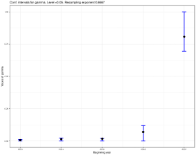
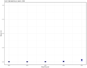
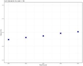
Figure 3: INE data. Estimations and confidence intervals for $\gamma$, $\pi$ and $\rho$. Level = 0.05

The first graph in Figure 3 and data in Table 5 show the values of the $\gamma$-index when comparing each year in the period 2003-2007 with the corresponding one four years later. They show that we can conclude that the status of all individual incomes in the initial date would be considered worse when considered in the final date except, at most, 2.23% of them in the periods 2003-07, 2004-08, and 2005-09. In the period 2006-10 the exception growths to 11.9%, and to 69.6% of individuals (and possibly for everybody) between 2007 and 2011.

Table 6 and second graph in Figure 3 show the results for the $\pi$-index. According to Proposition 2.5, the estimations in this table must be lower than those in Table 5 what is obviously true and the same happens with the extremes of all the confidence intervals. As explained before, the $\pi$-coefficient, instead of comparing quantiles against quantiles in the full Spanish population, addresses to the fact that there exist subpopulations, containing the $\pi\times 100\%$ of their respective original populations, which verify the dominance.

Here we want to pay special attention to the period 2007-11. According to the $\gamma$-index it happens that at least 69.6% of the percentiles are lower in the year 2007 than in 2011, thus giving a strong support to the worsening of the economical situation of the individuals.

However, the upper limit of the confidence interval of the $\pi$-index is just 0.045, and according to the reasoning in Remark 2.8, we should conclude that the global impoverishment was noticeable but not too severe.

In the remaining periods, there are not so big differences between both indices and, consequently, the interpretation is similar to that one we gave for the $\gamma$-index.

The index $\rho$ gives the probability that a Spanish individual randomly chosen, for instance, in 2003 has greater incomes than another one, independently chosen in 2007. Therefore, probabilities lower (resp. higher) than 0.5 hint to an improvement (resp. worsening) of the economical situation of the individuals. This reinforces previous comments about the fact that $\rho$ is a less informative index.

The results obtained from this index appear in Table 7 and last graph in Figure 3. From those data, in the sense already stated, we conclude that a general improvement in the conditions of the Spanish population happened in all four years periods starting on 2003 to 2006 while a worsening happened during the period starting on 2007 in agreement with the conclusions obtained with the $\gamma$-index.

4.2.2 NHANES data

This data set was obtained from NHANES (the U.S. National Health and Nutrition Examination Survey) and can be downloaded from https://doi.org/10.7910/dvn/shbf2g. We have considered individuals in growth age, from 2 to 14 years from the surveys in years 1999, 2001, 2003, 2005, 2007 and 2009. Sample sizes for every cohort by sex and age are shown in Table 3. The objective here is to analyze the dominance of the heights of boys over those of the girls.

Age	2	3	4	5	6	7	8	9	10	11	12	13	14
$n$ (boys)	796	632	633	563	557	582	579	543	556	556	735	728	704
$m$ (girls)	776	563	620	567	542	564	572	579	536	587	733	757	764

Table 3: Sample sizes by age (boys, top row; girls, bottom row)

The results of the computations appear in Tables 8, 9 and 10 in Subsection A.2 in the Appendix. A graphical representation of those results appears in Figure 4.

Concerning the $\gamma$-index, the results in Table 8 and left graph in Figure 4 show how the boys are clearly larger than the girls at 2, 4 to 6, and 14 years (to be more precise: all male percentiles in those ages are larger than the corresponding ones for girls excepting, at most, 2.05% of them. Thus, the status according to their height of 97.95% of the boys would improve if they were considered within the population of girls. The situation is reversed at 10 and 11 years (excepting, at most, for 6.82% of boys). For ages 7 to 9 and 12 and 13, where the transitions happen, the situation is somehow doubtful, in spite of we could accept that at age 8 boys look larger than girls because the proportion of percentiles which do not agree with that is, at most, 8.96%.

The age 3 looks a bit strange because it has an index similar to that one of age 8 but it is located in the middle of a period in which boys look taller than girls.

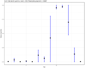
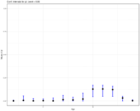
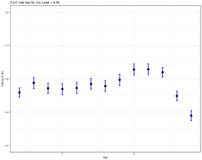
Figure 4: NHANES data. Estimations and confidence intervals for $\gamma$, $\pi$ and $\rho$. Level = 0.05.

Table 9 and the central graphic in Figure 4 show the results for the $\pi$-index. In general, the conclusions here are similar to those obtained when analyzing the $\gamma$-index, replacing proportion of people by sizes of subpopulations agreeing with the stochastic order.

It also gives the maximal difference in the status that a given height is getting in the boys population or in the girls one. However, we want to stress the situation in the ages 10 to 12 where the comments we made for the economical situation 2007-2011 apply.

Once again, the estimations of the $\pi$-indices are much lower that the corresponding to the $\gamma$-indices. However, this does not happen with the upper bounds for ages 2 and 5, where the upper bound of $\pi$ is slightly greater than the one of $\gamma$, and, mostly, for ages 14 (where it is at least, twice larger) and 4 and 6 (six times larger). This could be related to the conservative upper bound obtained for the index $\pi$, based on the worse variance possible, see details in Álvarez-Esteban et al. (2016), but also to the different rates of convergence and the sample sizes.

Values of the $\rho$-index lower than 0.5, lead to stochastic precedence in the sense of Arcones et al. (2002) (recall Section 2.2), (and the opposite for values greater than 0.5), thus the conclusions from Table 10 are in the same line than those for the $\gamma$ and $\pi$ indices.

4.2.3 HVTN data

This data set is owned by the HIV Vaccine Trials Network (HVTN). It was downloaded on January 27th, 2022 from the Shen et al folder at

https://atlas.scharp.org/cpas/project/HVTN%20Public%20Data/Cross-Protocol%20HVTN%20Manuscripts/begin.view

This data set is related to the comparison of the results of two different vaccine trials agains the HIV illnes: the so called HIV Vaccine Trials Networks (HVTNs) 097 and 100. The goal is to investigate to what extent the results of HVTN 097 stochastically dominates those of HVTN 100.

A very similar data set was analysed in Laha et al. (2021) to find an interval in which stochastic dominance happens. Regrettably the results are not comparable because the data set handled there shows some differences with the data set we have used here. It has become impossible to obtain the same data set used in Laha et al. (2021) because it is not publicly available.

We measure the effect of the vaccines in the same way as Laha et al. (2021) does, which the authors describe as follows:

“…[they] consider the magnitude of IgG binding to the V1V2 region of seven clade C glycoprotein 70 antigens. The immune responses were measured by an HIV-1 binding antibody multiplex assay (BAMA) …[using] the log-transformed net median fluorescence intensity (MFI) as the measure of immune response for statistical analysis.” We refer to Section 2 in Laha et al. (2021) for additional details.

The main difference with Laha et al. (2021) is in the problem statement: those authors select ‘by eye’ the interval in which HVTN 097 stochastically dominates HVTN 100 while here we apply a more objective method since it is the estimation of the index $\gamma$ (or $\pi$) who makes the selection.

Differences between the handled data sets are that, in our data set, there are 66 and 140 vaccines in the HVTN 097 and HVTN 100 trials respectively, while the data set handled in Laha et al. (2021) (see last paragraph in page 5) contains 68 and 180 vaccines in each trial; however, the main difference is an outlier that they have in the HVTN 097 sample which is the lower value in the experiment in theirs data. This outlier damages the dominance of HVTN 097 over HVTN 100.

The results obtained for the three indices handled in this paper appear in Table 4 and confirm the dominance of the vaccine HVTN 097 over HVTN 100: HVTN 097 dominates at least for 97.5% of the percentiles and the index $\pi$ shows that there exists a subpopulation composed by, at least 95.7% of the population in which this domination happens. The low value of the $\rho$-index corroborates those findings.

	Lower bound	Estimation	Upper bound
$\gamma$-index:	0.0000	0.0152	0.0249	(Upp. bound inv. speed: 4.0424)
$\pi$-index:	0.0000	0.0071	0.0429
$\rho$-index:	0.0480	0.1686	0.2892

Table 4: HVTN data. Estimations and confidence intervals for $\gamma$, $\pi$ and $\rho$ and upper confidence bound for the speed of convergence of $\gamma_{n,m}$. All of them at the level 0.05.

It is noticeable that, in this data set, the estimated value for $\pi$ is lower than the corresponding one for $\gamma$ (in fact, a half of it) as it must happen according to the definition of $\pi$; but, as it happened in some cases of NHANES data, the indeterminacy in the estimation of $\pi$ is larger than the indeterminacy in the estimation of $\gamma$, making the upper limit of the confidence interval for $\pi$ about 70% larger than this one for $\gamma$. This disagreement is probably due to the low sample size involved in this example.

Appendix A Appendix

A.1 Proof of Theorem 3.3

Without loss of generality we can assume that our samples, $\{X_{n}\}$ and $\{Y_{m}\}$, have been obtained from independent $U(0,1)$ samples $\{U_{n}\}$ and $\{V_{m}\}$ through the transformations $X_{i}=F^{-1}(U_{i}),Y_{j}=G^{-1}(V_{j}).$ We will denote the empirical quantile functions of the uniform samples by $\mathbb{U}_{n}$ and $\mathbb{V}_{m}$. We have the obvious relations

$$F_{n}^{-1}=F^{-1}(\mathbb{U}_{n}),G_{m}^{-1}=G^{-1}(\mathbb{V}_{m}).$$ (24)

With the usual notation $u_{n}$ and $v_{m}$ for the quantile processes based on the $U_{i}$’s and the $V_{j}$’s, respectively, ($u_{n}(t)=\sqrt{n}(\mathbb{U}_{n}(t)-t)$ and similarly for $v_{m}$) we have that

$$F_{n}^{-1}(t)=F^{-1}{\textstyle\Big{(}t+\frac{u_{n}(t)}{\sqrt{n}}\Big{)}}\ \mbox{ and }\ G_{m}^{-1}(t)=G^{-1}{\textstyle\Big{(}t+\frac{v_{m}(t)}{\sqrt{m}}\Big{)}.}$$ (25)

In an analogous way, we can obtain appropriate representations of the bootstrap distribution and quantile functions. By resorting to additional independent $U(0,1)$ samples $\{\tilde{U}_{n}\}$ and $\{\tilde{V}_{m}\}$ (and independent of the sequences above), and using the obvious modifications in the notation, (24) gives that

$$\tilde{F}_{\tilde{n}}^{-1}(t):=F^{-1}(\mathbb{U}_{n}(\tilde{\mathbb{U}}_{\tilde{n}}(t))),\ \ \ \ \tilde{G}_{\tilde{m}}^{-1}(t):=G^{-1}(\mathbb{V}_{n}(\tilde{\mathbb{V}}_{\tilde{m}}(t))),\ \ t\in[0,1],$$

which are versions of the bootstrap quantile functions associated to independent bootstrap samples, with resampling sizes $\tilde{n},\tilde{m}$, obtained without replacement of the original samples $X_{1},\dots,X_{n}$ and $Y_{1},\dots,Y_{m}$.

Let us now focus on $\tilde{F}_{\tilde{n}}^{-1}$. The iterated use of (25) leads to

$$\tilde{F}_{\tilde{n}}^{-1}(t)=F^{-1}\left(t+\frac{\tilde{u}_{\tilde{n}}(t)}{\sqrt{\tilde{n}}}+\frac{u_{n}\left(t+\frac{\tilde{u}_{\tilde{n}}(t)}{\sqrt{\tilde{n}}}\right)}{\sqrt{n}}\right),$$ (26)

where $\tilde{u}_{\tilde{n}}$ is the quantile process associated to a smaple with size $\tilde{n}$ taken from $\{\tilde{U}_{n}\}$.

The following result is a consequence of a refined version of the Komlos-Major-Tusnady construction (the Hungarian construction) for the quantile process (see, e.g., Theorem 3.2.1, p. 152 in Csörgo and Horvath (1993)), from which we know that there exists a sequence of Brownian bridges on $[0,1]$, $\{B_{n}\}$, versions of $u_{n}$ and positive constants, $C_{1},C_{2}$ and $C_{3}$, such that

$$P\Big{\{}\sup_{0\leq t\leq 1}|u_{n}(t)-B_{n}(t)|>{\textstyle\frac{x+C_{1}\log n}{\sqrt{n}}}\Big{\}}\leq C_{2}e^{-C_{3}x},\quad x>0.$$

Making use of this construction for the quantile processes $\tilde{u}_{\tilde{n}}$ and $\tilde{v}_{\tilde{m}}$, and taking $x=\frac{a}{C_{3}}\log n$ with $a>1$ and $K=\frac{a}{C_{3}}+C_{1}>0$, we obtain useful independent sequences of Brownian bridges $\{B_{\tilde{n}}^{1}\}$, $\{B_{\tilde{m}}^{2}\}$ and versions of $\tilde{u}_{\tilde{n}}$ and $\tilde{v}_{\tilde{m}}$, independent of the sequences of processes $u_{n}$ and $v_{m}$, as stated in the next theorem.

Theorem A.1

With the previous notation, in a probability one set, the sequences $\{B_{\tilde{n}}^{1}\}$, $\{B^{2}_{\tilde{m}}\}$, $\tilde{u}_{\tilde{n}}$ and $\tilde{v}_{\tilde{m}}$ eventually satisfy

$$\sup_{0\leq t\leq 1}|\tilde{u}_{\tilde{n}}(t)-B_{\tilde{n}}^{1}(t)|\leq{\textstyle K\frac{\log\tilde{n}}{\sqrt{\tilde{n}}}}\quad\mbox{ and }\quad\sup_{0\leq t\leq 1}|\tilde{v}_{\tilde{m}}(t)-B_{\tilde{m}}^{2}(t)|\leq{\textstyle K\frac{\log\tilde{m}}{\sqrt{\tilde{m}}}}.$$ (27)

Another consequence of the Hungarian construction and the functional law of iterated logarithm for the Kiefer process is the following law of iterated logarithm for the uniform quantile process (see, e.g., (3.3.2) in Theorem 3.1, p. 164 in Csörgo and Horvath (1993)):

$$\lim\sup\sqrt{\frac{2}{\log\log n}}\sup_{t\in[0,1]}|u_{n}(t)|=1\mbox{ a.s.}$$

Thus, there exists a constant $C$ and a probability one set such that

$$\frac{\sup_{t\in[0,1]}|u_{n}(t)|}{\sqrt{n}}\leq C\sqrt{\frac{\log\log n}{n}}\mbox{ eventually.}$$ (28)

If now, $f:[0,1]\to\mathbb{R}$ is any Lipschitzian function, relations (28) and (27) imply that, for a suitable $L$, the following inequality holds eventually in a probability one set

$$\sqrt{\tilde{n}}\left|f\left(t+\frac{\tilde{u}_{\tilde{n}}(t)}{\sqrt{\tilde{n}}}+\frac{u_{n}\left(t+\frac{\tilde{u}_{\tilde{n}}(t)}{\sqrt{\tilde{n}}}\right)}{\sqrt{n}}\right)-f\left(t+\frac{B^{1}_{\tilde{n}}(t)}{\sqrt{\tilde{n}}}\right)\right|\leq L\left(\sqrt{\frac{\tilde{n}\log\log n}{n}}+\frac{\log\tilde{n}}{\sqrt{\tilde{n}}}\right)$$ (29)

If the resampling size$\tilde{n}\to\infty$ and it satisfies $\tilde{n}=o(\frac{n}{\log\log n})$ as the sample size $n\to\infty$, relations (26) and (29) show that, if $F^{-1}$ is Lipschitz, then, the asymptotic behaviour of the processes $\sqrt{\tilde{n}}\left(\tilde{F}_{\tilde{n}}^{-1}(t)-F_{n}^{-1}(t)\right)$ and $\sqrt{\tilde{n}}\left(F^{-1}\left(t+\frac{B^{1}_{\tilde{n}}(t)}{\sqrt{\tilde{n}}}\right)-F_{n}^{-1}(t)\right)$ conditionally to $\{X_{n}\}$ are a.s. the same. In fact, since $\sqrt{n}(F_{n}^{-1}(t)-F^{-1}(t))$ converges in distribution, $\sqrt{\tilde{n}}(F_{n}^{-1}(t)-F^{-1}(t))\to 0$ in probability, and that behaviour is also the same as that $\sqrt{\tilde{n}}\left(F^{-1}\left(t+\frac{B^{1}_{\tilde{n}}(t)}{\sqrt{\tilde{n}}}\right)-F^{-1}(t)\right)$.

We can also elaborating with a view on the estimation of the parameter $\gamma$ in the following terms. Given two real functions $f$ and $g$ and versions of independent sequences of Brownian bridges $\{B_{\tilde{n}}^{1}\}$, $\{B_{\tilde{m}}^{2}\}$ and of independent uniform quantile processes, $u_{n}$, $\tilde{u}_{n}$, $v_{m}$ and $\tilde{v}_{m}$, as in Theorem A.1, we set

$$\begin{array}[]{rcl}{f}_{\tilde{n}}(t):=f\left(t+\frac{\tilde{u}_{\tilde{n}}(t)}{\sqrt{\tilde{n}}}+\frac{u_{n}\left(t+\frac{\tilde{u}_{\tilde{n}}(t)}{\sqrt{\tilde{n}}}\right)}{\sqrt{n}}\right)&\mbox{ and }&{g}_{\tilde{m}}:=g\left(t+\frac{\tilde{v}_{\tilde{m}}(t)}{\sqrt{\tilde{m}}}+\frac{v_{n}\left(t+\frac{\tilde{v}_{\tilde{m}}(t)}{\sqrt{\tilde{m}}}\right)}{\sqrt{m}}\right),\\[5.69054pt] \tilde{f}_{\tilde{n}}(t):=f\left({\textstyle t+\frac{B_{\tilde{n}}^{1}(t)}{\sqrt{\tilde{n}}}}\right)&\mbox{ and }&\tilde{g}_{\tilde{m}}:=g\left({\textstyle t+\frac{B_{\tilde{m}}^{2}(t)}{\sqrt{\tilde{m}}}}\right).\end{array}$$

The following lemma is the adaptation of Lemma 3.3 in del Barrio et al. (2021) to the present setup. Its proof follows the same arguments, with the additional already presented ingredients.

Lemma A.2

Consider $A\subset(0,1)$ such that $\ell(A)>0$. With the notation and construction above, let the resampling sizes satisfy $\tilde{n}=o(\frac{n}{\log\log n})$, $\tilde{m}=o(\frac{m}{\log\log m})$. If we assume that $f,g$ are two real Lipschitz functions, then there exists $L>0$ such that, if $C_{\tilde{n},\tilde{m}}:=L\left({\textstyle\frac{\log{\tilde{n}}}{\tilde{n}}+\frac{\log{\tilde{m}}}{\tilde{m}}+\sqrt{\frac{\log\log n}{n}}+\sqrt{\frac{\log\log m}{m}}}\right)$, then whenever $n,m\to\infty$, on a probability one set eventually,

$$\ell\big{\{}t\in A:\,\tilde{f}_{\tilde{n}}(t)>\tilde{g}_{\tilde{m}}(t)+C_{\tilde{n},\tilde{m}}\big{\}} \leq \ell\big{\{}t\in A:\,{f}_{\tilde{n}}(t)>{g}_{\tilde{m}}(t)\big{\}}$$

$$\leq \ell\big{\{}t\in A:\,\tilde{f}_{\tilde{n}}(t)>\tilde{g}_{\tilde{m}}(t)-C_{\tilde{n},\tilde{m}}\big{\}}.$$

As already noted, Lemma A.2 allows to replicate the proof of Theorem 4.9 in del Barrio et al. (2021) to obtain Theorem 3.3. It suffices to replace the role of Lemma 3.3, there, by the new lemma involving the bootstrap distributions.

A.2 Tables of Subsections 4.2.1 and 4.2.2

The complete values of the estimation of the indices $\gamma,\pi$ and $\rho$ for the INE-data appear in Tables 5, 6 and 7 and those corresponding to the NHANES-data are shown in Tables 8, 9 and 10 which are included next.

	Upper bound
Year	inverse speed	LowerBound	Estimation	UpperBound
2003	16.0869	0	0.0065	0.0117
2004	7.1981	0	0.0143	0.0233
2005	2.3412	0	0.0178	0.0220
2006	19.3965	0	0.0703	0.1190
2007	8.4167	0.6956	0.8079	1

Table 5: INE data. Estimations and confidence intervals for $\gamma$. Level = 0.05

Year	Lower Bound	Estimation	Upper Bound
2003	0	0.0019	0.0034
2004	0	0.0010	0.0038
2005	0	0.0025	0.0049
2006	0	0.0066	0.0139
2007	0.0178	0.0341	0.0447

Table 6: INE data. Estimations and confidence intervals for $\pi$. Level = 0.05

Year	LowerBound	Estimation	UpperBound
2003	0.3635	0.3721	0.3807
2004	0.4010	0.4097	0.4183
2005	0.4296	0.4385	0.4475
2006	0.4770	0.4859	0.4947
2007	0.5060	0.5148	0.5235

Table 7: INE data. Estimations and confidence intervals for $\rho$. Level = 0.05

	Upper bound
Age	inverse speed	LowerBound	Estimation	UpperBound
2	1.7170	0	0.0062	0.0076
3	31.5739	0	0.0346	0.0626
4	2.7928	0	0.0031	0.0044
5	3.0935	0	0.0140	0.0205
6	6.6794	0	0.0035	0.0059
7	16.1489	0	0.1176	0.2090
8	4.8127	0	0.0625	0.0896
9	265.4969	0	0.4217	0.8084
10	3.4711	0.9318	0.9549	1
11	4.3552	0.9563	0.9724	1
12	9.0628	0.4743	0.6999	1
13	14.0858	0	0.1374	0.2475
14	1.7431	0	0.0052	0.0065

Table 8: Nhanes data. Estimations and confidence intervals for $\gamma$. Level = 0.05

Age	Lower Bound	Estimation	Upper Bound
2	0	0.0013	0.0091
3	0	0.0066	0.0533
4	0	0.0016	0.0272
5	0	0.0036	0.0234
6	0	0.0014	0.0343
7	0	0.0145	0.0616
8	0	0.0110	0.0416
9	0	0.0211	0.0838
10	0.0445	0.1284	0.1716
11	0.0475	0.1297	0.1698
12	0.0501	0.1229	0.1603
13	0	0.0320	0.0511
14	0	0.0031	0.0137

Table 9: NHANES data. Estimations and confidence intervals for $\pi$. Level = 0.05

Age	Lower Bound	Estimation	Upper Bound
2	0.3626	0.3978	0.4330
3	0.4283	0.4696	0.5109
4	0.3900	0.4294	0.4687
5	0.3824	0.4237	0.4650
6	0.3897	0.4318	0.4738
7	0.4199	0.4611	0.5024
8	0.4048	0.4458	0.4867
9	0.4509	0.4929	0.5350
10	0.5279	0.5702	0.6125
11	0.5299	0.5715	0.6130
12	0.5135	0.5497	0.5859
13	0.3357	0.3720	0.4084
14	0.1871	0.2241	0.2610

Table 10: NHANES data. Estimations and confidence intervals for $\rho$. Level = 0.05

References

- (1)
- (2)
- Álvarez-Esteban et al. (2011) Álvarez-Esteban, P.C.; del Barrio, E.; Cuesta-Albertos, J.A. and Matrán, C. (2011). Uniqueness and approximate computation of optimal incomplete transportation plans. Annales de l’Institut Henri Poincaré - Probabilités et Statistiques 47, 358–375.
- Álvarez-Esteban et al. (2012) Álvarez-Esteban, P.C.; del Barrio, E.; Cuesta-Albertos, J.A. and Matrán, C. (2012). Similarity of samples and trimming. Bernoulli 18, 606–634.
- Álvarez-Esteban et al. (2014) Álvarez-Esteban, P.C.; del Barrio, E.; Cuesta-Albertos, J.A. and Matrán, C. (2014). A contamination model for approximate stochastic order: extended version. http://arxiv.org/abs/1412.1920
- Álvarez-Esteban et al. (2016) Álvarez-Esteban, P.C.; del Barrio, E.; Cuesta-Albertos, J.A. and Matrán, C. (2016). A contamination model for stochastic order. Test 25, 751–774.
- Álvarez-Esteban et al. (2017) Álvarez-Esteban, P.C.; del Barrio, E.; Cuesta-Albertos, J.A. and Matrán, C. (2017). Models for the assessment of treatment improvement: the ideal and the feasible. Statist. Sci., 32, 469–485. DOI: 10.1214/17-STS616
- Anderson (1996) Anderson, G. (1996). Nonparametric tests for stochastic dominance, Econometrica 64, 1183–1193.
- Arcones et al. (2002) Arcones, M. A., Kvam, P. H., and Samaniego, F. J. (2002). Nonparametric estimation of a distribution subject to a stochastic precedence constraint. J. Amer. Statist. Assoc. 97, 170–182.
- Arcones (2003) Arcones, M. A. (2003). On the asymptotic accuracy of the Bootstrap under arbitrary resampling size. Ann. Inst. Statist. Math.55(3), 563–583.
- Barrett and Donald (2003) Barrett, G.F., and Donald, S.G., (2003). Consistent tests for stochastic dominance. Econometrica 71, 71–104
- del Barrio et al. (2021) del Barrio, E., Cuesta-Albertos, J.A. and Matrán, C. (2021). The complex behaviour of Galton rank order statistic. Accepted by Bernoulli. Preprint at http://arxiv.org/abs/2102.02572.
- Berger (1988) Berger, R.L. (1988). A nonparametric, intersection-union test for stochastic order. In Statistical Decision Theory and Related Topics IV. Volume 2. (eds. Gupta, S. S., and Berger, J. O.). Springer-Verlag, New York.
- Bertail et al. (1999) Bertail, P., Politis, D. N., and Romano, J. P. (1999). On Subsampling Estimators with Unknown Rate of Convergence. J. Amer. Statist. Assoc. 94(446), 569–579. https://doi.org/10.1080/01621459.1999.10474151
- Birnbaum (1965) Birnbaum, Z. W. (1965). On a use of the Mann-Whitney statistic. In Proceedings of the Third Berkeley Symposium on Probability and Statistics, Vol. 1, 13–17. University of California Press.
- Chung and Feller (1949) Chung, K. L., and Feller, W. (1949). On fluctuations in coin-tossing. Proc. Nat. Acad. Sci. of USA, 35, 605–608.
- Csörgo and Horvath (1993) Csörgo, M. and Horvath, L. (1993). Weighted approximations in probability and statistics. Wiley.
- Davidson and Duclos (2013) Davidson, R., and Duclos, J.-Y. (2013). Testing for restricted stochastic dominance, Econometric Rev. 32, 84–125.
- Dette and Wied (2016) Dette, H., and Wied, D. (2016). Detecting relevant changes in time series models. J. R. Statist. Soc. B, 78(2), 371–394.
- Dette and Wu (2018) Dette, H., and Wu, w. (2018). Change point analysis in non-stationary processes - a mass excess approach. https://arxiv.org/abs/1801.09874.
- Feller (1968) Feller, W. (1968). An Introduction to Probability Theory and its Applications Vol. I (Third edition). Wiley.
- Govindarajulu (1968) Govindarajulu, Z. (1968). Distribution free confidence bounds for . Ann. Instit. Statist. Math. 20, 229–238.
- Gross and Holland (1968) Gross, S., and Holland, P. W. (1968). The Distribution of Galton’s Statistic. Ann. Math. Statist., 39(6), 2114–2117.
- Hodges (1955) Hodges, J. L.(1955). Galton’s rank-order test. Biometrika 42, 261–262.
- Hodges and Lehmann (1954) Hodges, J.L. and Lehmann, E.L. (1954). Testing the approximate validity of statistical hypotheses. J. R. Statist. Soc. B 16, 261–268.
- Kotz et al. (2003) Kotz, S., Lumelskii, Y., and Pensky, M. (2003). The Stress-Strength Model and its Generalizations. Theory and Applications. World Scientific Publishing.
- Laha et al. (2021) Laha, N., Moodie, Z., Huang, Y. and Luedtke, A. (2021). Improved inference for vaccine-induced immune responses via shape-constrained methods. ArXiv preprint: https://arxiv.org/pdf/2107.11546.
- Lehmann (1955) Lehmann, E. L. (1955). Ordered families of distributions. Ann. Math. Statist. 26, 399–419.
- Lehmann and Rojo (1992) Lehmann, E. L., and Rojo, J. (1992). Invariant directional orderings. Ann. Statist. 20, 2100–2110.
- Lehmann and Romano (2005) Lehmann, E. L., and Romano, J. P. (2005). Testing Statistical Hypotheses (Third edition). Springer.
- Leshno and Levy (2002) Leshno, M. and Levy, H. (2002). Preferred by “All” and preferred by “Most” decision makers: almost stochastic dominance. Management Sci. 48, 1074-1085
- Lindvall (1999) Lindvall, T. (1999). On Strassen’s theorem on stochastic domination. Electronic Communications in Probability, 4, 51–59.
- Linton et al. (2005) Linton, O., Maasoumi, E., and Whang, Y.-J. (2005). Consistent Testing for Stochastic Dominance under General Sampling Schemes. Rev. Economic Studies 72, 735–765.
- Liu and Lindsay (2009) Liu, J., and Lindsay, B.G. (2009). Building and using semiparametric tolerance regions for parametric multinomial models. Ann. Statist. 37, 3644–3659.
- Mann and Whitney (1947) Mann, H. B., and Whitney, D. R. (1947). On a test of whether one of two random variables is stochastically larger than the other. Ann. Math. Statist. 18, 50–60.
- McFadden (1989) McFadden, D. (1989). Testing for stochastic dominance. In Studies in the Economics of Uncertainty: In Honor of Josef Hadar, ed. by T. B. Fomby and T. K. Seo. Springer.
- Munk and Czado (1998) Munk, A., and Czado, C. (1998). Nonparametric validation of similar distributions and assessment of goodness of fit. J. R. Statist. Soc. B, 60, 223–241.
- Raghavachari (1973) Raghavachari, M. (1973). Limiting distributions of the Kolmogorov-Smirnov type statistics under the alternative. Ann. Statist. 1, 67–73.
- Rudas et al. (1994) Rudas, T., Clogg, C.C., and Lindsay, B. G. (1994). A new index of fit based on mixture methods for the analysis of contingency tables. J. R. Statist. Soc. B 56, 623–639.
- Sparre-Andersen (1953) Sparre-Andersen, E. (1953). On the fluctuations of sums of random variables. Math. Scand. 1, 263–285.
- Zhuang et al. (2021) Zhuang, W., Li, Y., and Qiu, G. (2021). Statistical inference for a relaxation index of stochastic dominance under density ratio model. Journal of Applied Statistics, https://doi.org/10.1080/02664763.2021.1965966
- Yu and Govindarajulu (1995) Yu, Q., and Govindarajulu, Z. (1995). Admissibility and minimaxity of the UMVU estimator of . Ann. Statist. 23, 598–607.
- Zhuang et al. (2019) Zhuang, W.W., Hu, B.Y., and Chen, J. (2019). Semiparametric inference for the dominance index under the density ratio model. Biometrika, 106, 1, 229–241