Power of Bonus in Pricing for Crowdsourcing

Abstract

We consider a simple form of pricing for a crowdsourcing system, where pricing policy is published a priori, and workers then decide their task acceptance. Such a pricing form is widely adopted in practice for its simplicity, e.g., Amazon Mechanical Turk, although additional sophistication to pricing rule can enhance budget efficiency. With the goal of designing efficient and simple pricing rules, we study the impact of the following two design features in pricing policies: (i) personalization tailoring policy worker-by-worker and (ii) bonus payment to qualified task completion. In the Bayesian setting, where the only prior distribution of workers’ profiles is available, we first study the Price of Agnosticism (PoA) that quantifies the utility gap between personalized and common pricing policies. We show that PoA is bounded within a constant factor under some mild conditions, and the impact of bonus is essential in common pricing. These analytic results imply that complex personalized pricing can be replaced by simple common pricing once it is equipped with a proper bonus payment. To provide insights on efficient common pricing, we then study the efficient mechanisms of bonus payment for several profile distribution regimes which may exist in practice. We provide primitive experiments on Amazon Mechanical Turk, which support our analytical findings.

1 Introduction

Crowdsourcing system is a popular tool to solve problems which involve huge amount of simple tasks, where the tasks are electronically distributed to numerous workers who are willing to perform the tasks at low cost. Once a task is given to workers, error is often common even among those who are willing due to low payment, tedium in tasks, and/or abundant spammers. To handle this, on one hand, a number of post-processing methods are developed to denoise dataset with some statistical inference techniques such as expectation maximization or belief propagation are applied to infer the correct answer to the task [DS79, RYZ⁺10, OOSY16]. However, there should be unavoidable limitations in guaranteeing a target precision when worker inputs are highly erroneous [FPCS06, GHG⁺14]. On the other hand, there have been an extensive line of studies on worker quality control, where workers are incentivized to submit better answers by the corresponding higher payment [MW10, CHK10]. Many experiments reveal that both the quantity and the quality of participants’ labels improve under the smart incentivization [BKG11, LRR15].

In many microtask crowdsourcing systems, a simple and eidetic pricing mechanism without bidding process is widely adopted due to the volatility of the incoming workers and characteristic of the tasks to be solved. For example in Amazon Mechanical Turk (MTurk), a task requester publishes a pricing rule a priori, based on which each worker decides on the task acceptance. Such workers are finally admitted to the system, if the requester has budget to pay them for their work. The following ideas are natural as possible ways to increase the requester’s utility: (i) personalized pricing that offers different rule to determine price for each individual worker and (ii) giving additional bonus to workers with more qualified task completion. Personalized pricing would be superior to the pricing without personalization (which we call common pricing throughout this paper). However, personalized pricing is obviously more complex and even cannot be adopted in some systems such as Mturk. A simple option of giving bonus to qualified workers in both personalized pricing and common pricing should provide more power in controlling workers’ behaviors which helps in increasing the requester’s utility. However, it has been underexplored how much gain personalization and/or bonus payment in pricing policies actually provide to the task requester.

The key message which we claim in this paper is that common pricing is enough when it is equipped with an appropriate choice of bonus payment, so as to catch two rabbits of simplicity and efficiency simultaneously. The main contributions to support our claim are summarized as follows:

1. Price of Agnosticism. We first study Price of Agnosticism (PoA) of a common pricing, which quantifies the gap between the optimal personalized pricing and a given common pricing (see Theorem 2). This PoA is expressed as $(\delta,\gamma)$-approximation, where $\delta\leq 1$ and $\gamma\geq 1$ correspond to the degree of approximations in terms of achieved utility and used budget, respectively, i.e., achieving $\delta U^{\star}_{p}(B)$ with $\gamma B$ budget, where $U^{\star}_{p}(B)$ is the maximum utility by the optimal personalized pricing for a given budget $B.$ We prove that there exists a common pricing which obtains the PoA $(1-o(1),O(1))$ for a large number of workers under some canonical scenarios.

2. Power of Bonus. We next study Power of Bonus (PoB) that explains the role of bonus payment in common pricing as a simple, yet powerful mechanism (see Theorem 3). We prove the necessity of bonus in common pricing in the sense that, without bonus, there always exists a worker profile distribution and arrival order under which any common pricing without bonus payment cannot achieve $(O(1),o(n))$-approximate to optimal pricing policy.

3. Optimal Common Pricing. For some canonical profile distribution regimes, we find the optimal structure of common pricing policies. Since the profile distribution can be interpreted as a consequence developed by the characteristic of task the requester is trying to solve along with the corresponding behavior of the workers, these results give some insights in designing the pricing policies with respect to the requester’s task.

4. Experiments. To validate our findings and draw practical implications, we numerically analyze the various profile distribution regimes and efficient structure of pricing policy, and execute a real-world experiment on Amazon Mechanical Turk, a popular crowdsourcing platform. The results from experiments verify the theoretical result on PoA, PoB, and the efficiency of some bonus structures, and it also gives some intuitions on how to build an efficient pricing policy given the requester’s utility function.

To sum up, our analytical and experimental results imply that a simple common pricing equipped with bonus payment is enough with no need of personalized pricing, and provide some useful insights in efficient form of pricing policies with respect to the crowdsourcing scenario.

In Section 2, we introduce our model and pricing mechanism, and in Section 3, we provide our main analytical results on PoA, PoB along with some case studies on worker regime. In Section 4, we provide the numerical results to verify the theoretical findings, and in Section 5, we provide the experimental results based on the real-world crowdsourcing data on Mturk. All the proofs are provided in Appendix.

1.1 Related Work

In this section, we provide an overview of literatures related to pricing mechanisms for microtask crowdsourcing systems, in which we want to incentives quality workers under budget constraints.

Pricing mechanisms with budget feasibility

We first present the work on pricing mechanism in crowdsourcing that is based on a procurement auction under budget feasibility constraint, i.e. budget feasible mechanism design. [Sin10] initiatively shows that for a general buyer utility function, standard mechanism design ideas such as VCG mechanism along with its variants cannot guarantee a constant-approximation to an optimal mechanism, while it becomes possible for certain classes of submodular utility functions. [AGN14] study the analogous problem under large market assumption, and [BCGL12] study the same problem under subadditive function in both prior-free and Bayesian framework.

Despite of the advantages of sealed-bid mechanism, they are rarely adopted in microtask crowdsourcing platforms due to the complex bidding process. However, posted pricing is widely used due to its simplicity [AKS19, SM14, Sek16, ZH17]. In this context, [BH16] define a Bayesian budget-feasible posted pricing, where given a prior knowledge on individual worker’s cost distribution, the buyer tries to maximize her expected utility within a fixed ex-post budget constraint. [HHL16, HHL18] study the Bayesian posted pricing mechanism under the prior knowledge in joint distribution of worker’s cost and quality, and formulate the problem as a budget minimization problem under robust quality constraint. We study a variant of budget feasible posted price mechanism, where the requester incentivizes the participants by giving a bonus payment based on the observed quality in addition to a participation fee.

Quality-based pricing and strategic behavior of workers

Since we integrate the concept of quality-based payment in posted price mechanism, we introduce some works studying on the strategic behavior of workers against the performance-based contract in labor market along with its difference from our model, and discuss why our model practically fits in our application. The literature of principal-agent problem [LM09, BFN06, Car15, LV02] addresses the question of incentivizing strategic workers based on their observed output, where the main focus is to design a contract to elicit costly efforts from strategic agents. In here, each agent strategically decides an effort level to exert on the task to maximize own payoff, where higher effort induces large opportunity cost but possibly large reward, and lower effort would not make much reward but it takes a small opportunity cost. There exists a number of works studying the crowdsourcing system in the context of principal-agent problem [HSV16, BNG⁺14, CWLZ19, MGLH18, HSSV15]. Meanwhile, there have been reported some empirical evidences that the workers in microtask crowdsourcing platforms do not strategize their effort level or induced quality, but only decide whether or not to participate in the requested task [JKC10, KR12, MW09]. In this context, the authors in [EG15, GK14] capture these characteristics of worker behavior, namely endogenous participation and exogenous quality, to model the real-world crowdsourcing platform and reveal the structure of efficient mechanism. Our work also considers an analogous intrinsic worker behavior, but in a budget-constrained scenario under posted price mechanism to capture the characteristic of the microtask crowdsourcing platform.

Price discrimination

Our main message is that differentiating pricing policy between workers is not necessary if its equipped with proper bonus payment in microtask crowdsourcing platform. In this sense, we explain the concept of price discrimination, why it is needed in terms of system utility, and introduce some works on studying the performance of system under less price discrimination. Firstly, price discrimination refers to the selling strategy that changes its offering price for different individual customers based on their observable features such as willingness to pay, or the utility they provide to the requester. It is an effective tool, or sometimes inevitable for recruiting qualified participants while filtering out poor ones which leads to higher requester utility, as used in extensive mechanism design literature [CHMS10, BH16, HHL16, HHT⁺17, CDHW20]. However, it is also widely known that differentiating pricing policy would possibly result in a negative effect on platform in long-term manner [AS10]. In this context, there exists a line of works on studying the performance of system without or less discrimination under monopoly provider scenario [EGH18, BCW19, BBM15], or under the presence of network externalities [HMW19]. We also address how the requester can effectively allocate the budget to workers without differentiating the pricing policy in microtask crowdsourcing platform, and reveal that if there exists no discrimination at all, then the performance of requester drops significantly, however, with implicit price discrimination occurred by proper quality-based bonus payment, the requester can achieve a near-optimal performance compared to pricing policy with both explicit discrimination via differentiation and implicit discrimination.

Common pricing in various applications

Finally, an extensive literature has studied the efficiency of common pricing policy, i.e. pricing without personalization, and how to design an efficient common pricing policy under practical applications. [BJR15] address the problem of designing pricing strategy for ride-sharing platforms, and reveal that under a reasonable condition, dynamic pricing that varies over time does not outperform fixed pricing. In contrary, [CKW17] show that fixed pricing suffers from a problem called wild goose chase, while the dynamic pricing solves it. [TWZ⁺18] consider the problem of spatial crowdsourcing and show that there exists an efficient dynamic pricing policy that significantly out-performs common pricing policy. In context of cloud pricing, [ZJWB⁺16] study the problem of computing an optimal profit-maximizing fixed price for cloud virtual service provider. The authors in [AKK12, DS21, ZJWT⁺15, SG20] consider the spot price exploited in Amazon Web Service, and study the profit of platforms and users under intersectional scenario where fixed pricing and spot pricing exist. Likewise, we study the efficiency of common pricing for microtask crowdsourcing platform, and provide the optimal structures of common pricing policies for some canonical regimes.

2 Model and Problem Formulation

2.1 System Model

We consider a set $\mathcal{N}=\{1,2,\ldots,n\}$ of workers, where $n$ is the number of workers who are available for a target task requested by the requester. Each worker $i\in\mathcal{N}$ is associated with a private profile $(s_{i},c_{i})\in\mathbb{R}_{\geq 0}^{2}$: she produces the output of quality $s_{i}$ at cost $c_{i}$ if she decides to perform the task, where $s_{i}$ and $c_{i}$ quantify the individual contribution to the task and the opportunity cost to perform the task, respectively. We adopt a standard Bayesian setting [HHL16]: the requester is aware of the prior distribution $f_{i}(s_{i},c_{i})$ for each $i\in\mathcal{N}$. We denote $x_{i}=1$ if worker $i$ decides to work on the task and $x_{i}=0$ otherwise. Let $\bm{s}:=[s_{i}]_{i\in\mathcal{N}}$ and $\bm{c}:=[c_{i}]_{i\in\mathcal{N}}$. Then, the task requester has utility $u(\bm{s}\circ\bm{x})$ for some function $u:\mathbb{R}_{\geq 0}^{n}\mapsto\mathbb{R}_{\geq 0}$, where $\bm{s}\circ\bm{x}=[s_{i}x_{i}]_{i\in\mathcal{N}},$ a function of the collection of the qualities of task-accepting workers.

Quality-based pricing

We consider a variant of budget feasible posted pricing framework where a quality-based pricing policy is posted in advance of workers’ arrival . Note that it is often called as performance-based pricing in the literature [Sha02]. In quality-based pricing, an extra payment is made as bonus to workers who produce good-quality outputs in addition to a base payment which is paid to workers irrelevant to their quality. We denote by $p:=[(p_{i})]$ a pricing policy, where each worker $i\in\mathcal{N}$ is offered $p_{i}$ consisting of an increasing function $p_{i}:\mathbb{R}_{\geq 0}\mapsto\mathbb{R}_{\geq 0}$ so that if worker $i$ accepts $p_{i}$ and submits an output $s_{i}$, she will be paid $p_{i}(s_{i})$. To interpretational simplicity, we refer to the constant term of $p_{i}$ as a base payment, and the others as a bonus payment. We assume that the workers strategically decide whether or not to accept the task [EG15, GK14]. Then, the requester’s objective is to find an optimal pricing policy $p$ that maximizes the expected utility for a given prior distribution $[f_{i}]$ of worker profile, while the choice of pricing policies can be restricted due to some practical constraints. We remark that incentivizing a worker based on her quality could be either straightforward or requiring some additional process depending on the task. For example in crowdsensing task, the requester might naturally have a method to estimate the quality of submitted sensing data. On the other hand, the requester can indirectly estimate $s_{i}$ by embedding golden questions with known answers purely for estimation, or delaying payment until the estimation on quality via some inference algorithms becomes accurate [DS79, RYZ⁺10, OOJ⁺19], while allocating tasks to a conservative number of workers. For example in case of binary classification task, it is known that the classification error rate of belief propagation decreases exponentially on the number of workers per task, under a reasonable regime of fairly good workers whose average probability to provide correct response is greater than $0.5$ [OOSY16, KOS14]. In most cases, task requesters anyway perform a denoising process to obtain clean labels, in which worker quality can be simply assessed by comparison between the denoised labels and worker’s responses, or a part of the denoising process.

Personalized and common pricing

We classify pricing policies into two types: (i) personalized pricing and (ii) common pricing, depending on whether pricing is discriminatory between each worker or not. In personalized pricing, different pricing policy $p_{i}$ can be applied for different worker $i,$ while common pricing is the one which applies the same pricing function $p$ to all workers. Thus, we denote a common pricing $p$ to be one with $p_{i}=p$ for each $i\in\mathcal{N}$. Note that the set of all common pricing policies is a subset of all personalized pricing policies. Despite personalized pricing policy’s more controllability on workers’ behavior and thus more expected utility to the requester, common pricing seems more useful, since personalized pricing is often discouraged in practice. For example, Amazon Mechanical-Turk [Tur18] utilizes a common pricing. Also, even after the price to be posted is determined, personalized pricing still needs to observe each incoming worker to offer the customized price, leading to higher system complexity and privacy concerns which possibly hinder the workers from participation [AS10]. However, common pricing needs only a summarizing property of the entire worker profiles rather than individual ones, implying that common pricing requires no information on each incoming worker after the price to be posted is determined. Note that even under common pricing a certain form of price differentiation is played as an incentive, depending on how good each worker is. However, such a payment function is not differentiated across the workers, which is the key difference from personalized pricing.

Worker behavior

Given a pricing policy $p$ and worker profile $\bm{s}$ and $\bm{c}$, we assume that each worker is rational so that worker $i$ strategically maximize her quasi-linear payoff $p_{i}(s_{i})-c_{i}$. More formally, worker $i$’s strategic decision on the task participation is made by:

$$\phi_{i}{(p_{i})}\mathrel{:=}\mathbbm{1}[p_{i}(s_{i})\geq c_{i}],$$ (1)

where $\mathbbm{1}[A]$ is the indicator function of $A,$ i.e., $\mathbbm{1}[A]$ is $1$ if $A$ is true, and $0$ otherwise, i.e., worker $i$ accepts the task when $\phi_{i}=1,$ and rejects otherwise. However, the final task allocation is determined depending on the available budget and the order of worker arrivals, as explained in what follows. We assume that workers arrive in a given but latent ordering $\sigma$ drawn over all possible orderings of $\mathcal{N}$. We note that our main results are based on the worst case analysis with respect to the ordering. Then, for given budget $B$, arrival model $\sigma$ and pricing policy $p$, task allocation vector $\bm{x}$ is determined in the following manner, as in [BH16]:

1. Worker $i$ arrives with profile $(s_{i},c_{i})$ with respect to ordering $\sigma$.

2. If the remaining budget is smaller than worker $i$’s maximal possible reward, then discard the worker.

3. Else, offer her $p_{i}(s_{i})$ and she accepts if her actual reward $p_{i}(s_{i})$ is larger than or equal to her cost $c_{i}$, and get paid $p_{i}(s_{i})$ and mechanism deducts it from the remaining budget. Otherwise, discard worker $i$.

Let $\mathcal{P}(p,B,\sigma)$ be the (random) process generating a task allocation vector $\bm{x}$ under pricing policy $p$ and budget constraint $B$, where we denote $\bm{x}\sim\mathcal{P}(p,B,\sigma)$. Note that the randomness in $\bm{x}$ comes from that of $\bm{s}$ and $\bm{c}.$ Under process $\mathcal{P}(p,B,\sigma)$, after the entire budget is exhausted, any incoming worker $i$ is naturally discarded and has $x_{i}=0$ even if she wants to participate in the task, i.e., $\phi_{i}(p_{i})=1.$ Hence, any realization $\bm{x}$ verifies the ex-post budget constraint [BH16], i.e.,

$$\sum_{i\in\mathcal{N}}p_{i}(s_{i})x_{i}\leq B\;.$$ (2)

We assume that $B=\Theta(n)$ to avoid the trivial arguments. For given pricing policy $p$ and budget $B$, we define the following expected utility (in the ex-post setting):

$$U(B;p):=\mathbb{E}_{\bm{x}\sim\mathcal{P}(p,B,\sigma)}[u(\bm{s}\circ\bm{x})].$$ (3)

2.2 Problem Formulation

For given $B\geq 0$, the problem of finding an optimal personalized pricing, referred to as OPP, is defined by:

OPP$$(B) \underset{p=[p_{i}]}{\textnormal{max}}\ U(B;p)$$: (4)

In general, we call an instance of the above problem with different parameter an optimal personalized pricing problem throughout this paper. Our goal is to investigate how feasible it is to employ a simple common pricing instead of an optimal personalized pricing. As earlier discussed, the payment function can be personalized to each worker’s profile, while a common pricing $p_{i}=p$ for $i\in\mathcal{N}$ is forced to be indistinguishable for all workers. Due to such controllability difference, the optimal personalized pricing naturally outperforms any optimal common pricing.

In both personalized and common pricing, the following tensions exist: If the requester sets high base and low bonus, it may fail to recruit high-quality users and utilize only low-cost users. If bonus is set too high with low base, it should spend a huge amount of bonus on high quality users, so that the total number of recruited users shrinks. Thus, it is necessary to strike a good balance between base and bonus payments while satisfying the budget constraint to maximize the achieved utility.

3 Main Results

In this section, we present our main results which are summarized as the following two key messages: (i) a simple common pricing can approximate an optimal personalized pricing well, when an appropriate bonus mechanism becomes available and (ii) without bonus payment, no common pricing can achieve an reasonable approximate to optimal personalized pricing. In addition, we provide some useful insights on the effective structure of pricing policy with respect to the characterization of the crowdsourcing task.

Additive utility

In our analytical results, we consider a canonical class of utility functions: additive mainly for mathematical tractability. We say that $u(\cdot)$ is additive if

$$u(\bm{s}\circ\bm{x})=\sum_{i\in\mathcal{N}}s_{i}x_{i}.$$ (5)

Although our theoretical understanding in this section assumes additivity mainly for tractability, we provide the experimental results which suggest similar implications for other utility functions. It is worth to note that even with additive utility, finding the optimal personalized pricing is computationally challenging:

Theorem 1.

OPP with additive utility is NP-hard.

The detailed proof is provided in Appendix, where we reduce classical knapsack problem, a well-known NP-hard problem, to a special case of OPP.

Reasonable workers

For analytical tractability, we assume that workers have reasonable value at their labor so that their quality given cost is upper bounded by a constant, formally the maximal value of the support of the random variable $s_{i}/c_{i}$ is constant, i.e. for every $i\in\mathcal{N}$, $\mathbb{P}[s_{i}/c_{i}<C]=1$ for some constant $C$. The assumption is very true in practice due to human’s limited capacity. In addition, without this assumption, a simple policy hiring only unreasonably low-cost workers with unbounded $s_{i}/c_{i}$ easily achieves a certain level of utility and thus devising efficient policy would not be meaningful in practice.

3.1 Price of Agnosticism and Power of Bonus

We now present our result that there exists a common pricing scheme whose performance is not far from that of an optimal personalized pricing. Our results are two-fold. First, we prove that there exists a simple, common pricing which produces a good approximation of OPP (small price of agnosticism, see Theorem 2). Second, we show that there always exists a worker distribution and worker arrival under which any common pricing without bonus perform poorly (large power of bonus, see Theorem 3).

$(\delta,\gamma)$-Approximation

To formally discuss, we first define a notion of approximate solution given by a common pricing to OPP(B):

Definition 1.

For a given budget $B\geq 0$ and worker distribution $[f_{i}]$, consider an optimal personalized pricing problem $\text{\em OPP}(B)$ in (4), and let $p^{\star}(B)$ be an optimal personalized pricing of $\text{\em OPP}(B)$. For $0\leq\delta\leq 1$, and $1\leq\gamma$, a common pricing $p_{c}$ is $(\delta,\gamma)$-approximate to OPP$(B)$ if

$${U}(\gamma B;p_{c})~{}\geq~{}\delta\times{U}\left(B;p^{\star}(B)\right).$$

The constants $\delta$ and $\gamma$ assess the suboptimality in terms of utility and budget, respectively. Intuitively, $p_{c}$ is able to achieve the utility of $\delta\times$ (utility by an optimal personalized pricing with budget $B$) with budget $\gamma B.$ Note that $(1,1)$-approximation corresponds to the exact optimality.

Price of Agnosticism

We first study Price-of-Agnosticism (PoA) that quantitatively compares personalized and common pricing policies, revealing how good a simple common pricing with bonus payment is, compared to the best personalized one.

We present Theorem 2 which states the existence of a common pricing which is a good approximation of an optimal personalized pricing, i.e., small price-of-agnosticism, as the number of workers $n$ grows.

Theorem 2 (Price-of-Agnosticism).

There exists a common pricing $p_{c}$ that is $\left(1-O(e^{-n^{1/6}}),O(1)\right)$-approximate to OPP$(B)$.

This theorem indicates that we can find a common pricing endowed with an appropriate bonus function that is a $(1,O(1))$-approximate to the optimal personalized pricing with bonus, which indeed implies that one can design an approximately optimal pricing policy without any explicit pricing differentiation across the workers. This is quite surprising since it even holds when the worker’s profile distributions are somewhat heterogeneous. It mainly springs from our assumption on reasonable workers which bounds the heterogeneity of the workers so that we can guarantee the approximately optimal utility within a slightly augmented budget.

We briefly summarize the key challenges and the issues in analysis. First, the major challenge in the proof is due to the tight correlation between task allocation and ordering of worker arrivals which the ex-post budget constraint creates. In order to bypass this challenge, we first consider a tractable yet perhaps artificial budget constraint, referred to as the ex-ante budget constraint [BH16]. Then, we establish the approximation ratio of $p_{c}$ under such ex-ante constraint by comparing it with an offline oracle algorithm in a fractionally relaxed version. Finally, we connect the ex-ante approximation ratio to the ex-post one using the concentration inequalities for contention resolution scheme under the knapsack constraint [VCZ11].

Specifically, we consider a class of linear pricing policy, i.e. $p(s_{i})=x+ys_{i}$ for some parameter $x,y\in\mathbb{R}$. Efficiency of linear pricing is quite intuitive since linear pricing naturally recruits only efficient workers whose quality-to-cost ratio $s_{i}/c_{i}$ is at least some threshold, resulting in a cost-effective allocation of the budget in additive utility case. We note that linear pricing is revisited along with other pricing policies in Section 4.

We note that the offline oracle algorithm in the fractionally relaxed version actually outperforms OPP, where it is assumed to have the knowledge on the incoming worker’s realizations of cost and quality along with their arrival order in advance, and also more controllability on the allocation vector. Thus, we conjecture that the actual performance between $p_{c}$ and OPP would be closer, and hence the gap between OPP and optimal common pricing would be much closer.

Power of Bonus

We next study the role of bonus payment in common pricing. Intuitively, a common pricing without bonus has no ability to prevent spammers from cherry picking: taking the (base) payment for low quality job. In the following theorem, we demonstrate how vulnerable the common pricing without bonus payment can be to cherry picking.

Theorem 3 (Power of Bonus).

There exists a worker profile distribution $[f_{i}]$ and worker arrival $\sigma$ such that no common pricing without bonus is $(\delta,o(n))$-approximate to OPP($B$) for any $\delta\in[0,1]$.

Hence, without the bonus structure in pricing policy nor personalization, there always exists a problem instance that the requester suffers from any constant amount of utility loss even with budget augmented upto any $n^{1-\varepsilon}$ for any $\varepsilon>0$. The sketch of the proof is as follows. To obtain this arbitrarily worst-case result, we mainly consider a “spammer-hammer” scenario in terms of worker qualities under the same cost (i.e., $c=c_{i}$ for all worker $i$), where we can always construct any common pricing without bonus that has arbitrarily poor performance even with additional budget by factor $o(n)$. This is intuitive, because as the quality gap between spammer and hammer increases, the need of price discrimination such as bonus grows accordingly. This also implies that employing bonus payment is crucial for obtaining good approximation of common pricing to the optimal personalized pricing that is even computationally intractable.

We note that the benefit of bonus can differ depending on information about worker profile. First, when we know each worker’s profile exactly, it is possible to design an optimal personalized pricing without bonus, which offers the minimal payment to engage workers. Hence, if individual worker’s profile and personalized pricing are available (although both of them are typically unavailable in practice), there is no need to use bonus payment. On the other hand, in the case that the profile distributions are not deterministic but the workers are homogeneous, i.e. $\bm{s},\bm{c}$ are identical for all workers, it is obvious that there is no gain at all from differentiating pricing policy between workers. Meanwhile, bonus payments might give some amounts of gain, we highlight that the power of bonus is larger than that of personalization in this case.

3.2 Profile Distribution and Optimal Common Pricing

We now study what an effective structure of bonus function for common pricing is, in three regimes of profile distribution. Each regime corresponds to different type of tasks.

Ratio-equivalent regime and linear pricing

Consider tedious tasks such as filtering out the spam mails, correcting the typos on some elementary-level articles, or classifying the animals from images. The worker quality is linearly proportional to her effort and time. Hence, the ratio between the cost and quality would be the same across the workers. Formally, we define ratio-equivalent regime such that $\mathbb{P}[c_{i}=ks_{i}]=1$ for every $i\in\mathcal{N}$ and for proportional constant $k\in\mathbb{R}_{\geq 0}$. We next define a linear-pricing with parameter $\alpha$ as the following:

$$\text{linear-pricing:}\quad p_{lin}(\alpha)=\alpha s_{i}$$

Note that it is a common pricing policy regardless of the parameter $\alpha$. We find that $p_{lin}(\cdot)$ with proper parameter exactly achieves the optimality in this case as follow:

Proposition 1.

Under ratio-equivalent regime with proportional constant $k$, linear-pricing $p_{lin}(k)$ is asymptotically optimal, meaning that $p_{lin}(k)$ achieves $(1,1)-$approximate to OPP(B) as $n$ goes to infinity.

The requester’s fundamental goal can be translated into recruiting the workers with higher marginal utility-to-cost ratio, i.e. $s_{i}/c_{i}$. Since the linear bonus function naturally achieves this goal in additive utility function, by recruiting the workers in the descending order of $s_{i}/c_{i}$, we expect that linear bonus equipped with a proper base payment would behave well in practice.

Cost-equivalent regime and threshold pricing

SETI [SET18] crowdsources computation resource, where the only thing participant needs to do is just setting a specific screen saver on computer, and thus the effort to participate is almost identical across the entire workers while each worker’s contribution is different depending on the specification of computers. This motivates us to define cost-equivalent regime such that $\mathbb{P}[c_{i}=c_{0}]=1$ for every $i\in\mathcal{N}$ and for some $c_{0}\in\mathbb{R}_{+}$. For this regime, we consider the following form of common pricing with parameters $\alpha,\beta$:

$$\text{threshold-pricing:}\quad p_{thre}(\alpha,\beta)=\alpha\mathbbm{1}[s_{i}\geq\beta]$$

In here, $\alpha$ denotes the amount of bonus payment, and $\beta$ denotes the threshold of worker quality to grant the bonus payment, where $\beta$ controls for whom we need to grant the bonus, and $\alpha$ controls how much to motivate those qualified workers. The following proposition implies that under the cost-equivalent regime, $p_{thre}(\cdot)$ with proper parameter is optimal:

Proposition 2.

Under cost-equivalent regime, threshold-pricing $p_{thre}(c_{0},\beta_{B})$ is asymptotically optimal for $\beta_{B}=\sup\left\{\beta\geq 0:\sum_{i\in\mathcal{N}}\mathbb{P}[s_{i}\geq\beta]\geq B/c\right\}$.

This is quite intuitive since in cost-equivalent regime, any optimal pricing policy needs to offer exactly the same price to every worker and hires the worker in the order of higher quality, where threshold pricing naturally achieves it.

Quality-equivalent regime and effect of bonus

We define quality-equivalent regime such that $\mathbb{P}[s_{i}=s_{0}]=1$ for every $i\in\mathcal{N}$ and for some $s_{0}\in\mathbb{R}_{\geq 0}$. As an example corresponding to this regime, one can consider survey asking non-trivial question, e.g., Moral Machine [Mor18] collecting people’s decision on a moral dilemma, where each individual’s contribution is counted as just a single answer regardless of the depth of thinking which may differ person-by-person significantly. We provide the following proposition which implies we can always transform any common pricing into common pricing without bonus with the same expected utility.

Proposition 3.

Under quality-equivalent regime, for any common pricing $[p(s_{i})]$, there exists a common pricing without bonus $[(p^{\prime}(s_{i}))]$ such that $p^{\prime}(s_{i})=\nu$ for some $\nu\in\mathbb{R}_{\geq 0}$ and $U(B;p)=U(B,p^{\prime})$.

If there exists no difference in worker quality, the requester just need to recruit any workers in the cheapest manner and this can be done without any bonus payment, which implies that there exists no gain from exploiting bonus payment in this regime. Note that we’re not claiming that bonus payment harm the requester’s utility, but there is no need of adopting bonus payment.

4 Simulation

In this section, we numerically analyze the utility of various common pricing along with in terms of their PoAs and PoBs, and verify the structure of efficient common pricing structure with respect to the profile distributions.

4.1 Setup

We consider 100 workers and two regimes of cost distributions of worker cost $c_{i}$, where for Figure 1LABEL:sub@fig:sim_linear and 1LABEL:sub@fig:sim_affine, cost of each worker $i$ is drawn uniformly at random from $[0.3,0.7]$, and for Figure 1LABEL:sub@fig:sim_uniform, cost of every worker $i$ is $0.5$ in deterministic manner. For each figures, we consider a mixture of two types, spammer and hammer, of worker quality where Spammer is a worker with $s_{i}=0.1$, and Hammer consists of the following 3 sub-types of worker’s quality distribution: (Linear) $s_{i}=c_{i}$, (Affine) $s_{i}=c_{i}-0.1,$ and (Uniform) $s_{i}\sim U[0.3,0.7]$, i.e. uniformly randomly drawn over $[0.3,0.7]$. The budget is set to be $30,$ and we choose the additive utility function of the requester $u(\bm{s}\circ\bm{x})=\sum_{i\in\mathcal{N}}s_{i}x_{i}.$ Depending on the type of bonus payment and the value of base payment, we consider different common pricing schemes. First, $x$-linear pricing represents pricing policy form of $p(s_{i})=x+ks_{i}$ for some bonus constant $k$. Next, $50\%$-thre(shold) pricing is defined as $p(s_{i})=k\mathbbm{1}[s_{i}\geq 0.5]$ so that it incentivizes the worker only if her quality is at least some threshold for some bonus constant $k$. For both pricing policies, we choose the bonus constant $k$ so that the expected utility becomes the largest over every pricing policy with the corresponding form. No-bonus pricing is the optimal one among the common pricing without bonus payment. Finally, we compute the expected utility of OPP in a brute-force manner, which was possible thanks to the constrained form of profile distributions and a reasonable number of workers. Finally, in Figure 1LABEL:sub@fig:sim_linear all the workers are of the types of spammer or linear, where the proportion of linear workers increase from $0\%$ to $100\%$, Figure 1LABEL:sub@fig:sim_affine corresponds to the case of spammer and affine workers, and Figure 1LABEL:sub@fig:sim_uniform corresponds to the case of spammer and uniform workers with equivalent cost.

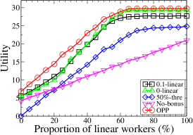
(a)

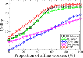
(b)

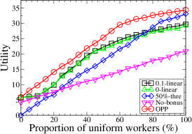
(c)

Figure 1: (a) Expected utility of pricing policies with respect to the proportion of linear workers in spammer-linear scenario. $0\%$ means that all the workers are spammers. (b) Expected utility of pricing policies with respect to the proportion of affine workers in spammer-affine scenario.(c) Expected utility of pricing policies with respect to the proportion of uniform workers in cost-equivalent spammer-uniform scenario.

4.2 Evaluation

Price of agnosticism and power of bonus

In Figure 1LABEL:sub@fig:sim_linear and 1LABEL:sub@fig:sim_affine, we observe that linear pricing has a good match with OPP, and in Figure 1LABEL:sub@fig:sim_uniform, threshold pricing achieves almost the optimum without any auxiliary budget. It implies that price of agnosticism is small when the pricing policy is appropriately designed, as we analyzed in Section 2. Next, we observe that the expected utility of No-bonus is very small, compared to those with bonus for both scenarios, where it supports the importance of bonus, as stated in Theorem 3. Finally, we highlight that in order to utilize the power of incentivization, it’s important to design the bonus function properly with respect to the profile distributions, since threshold pricing performs even worse than No-bonus for spammer regime in Figure 1LABEL:sub@fig:sim_linear.

Choice of base payment

In Figure 1LABEL:sub@fig:sim_affine, it is interesting to see that pricing policies with base $0.1$ have larger expected utility than that with zero base payment. For a linear pricing to achieve near-optimal utility without any augmented budget, it needs to reduce its budget waste caused by redundant bonus payment. To this end, every worker needs to output exactly proportional to what the requester paid, i.e., outputs $0.2$ if she gets paid $\$0.2$, outputs $0.4$ for $\$0.4$. For affine workers, $0$-linear fails to do so due to the negative bias introduced in the affine profile distribution. For example, if $0$-linear pays $2\cdot s$ bonus, then it pays $\$0.4$ for worker with profile $(s,c)=(0.2,0.4)$, but it pays $\$0.8$ for worker with profile $(s,c)=(0.4,0.6)$, i.e., the budget is wasted on this worker which leads to the utility decrement as shown in Figure 1LABEL:sub@fig:sim_linear. However, if some amount of the base payment is ready, it helps to recover the negative bias in affine workers, so that they output exactly as they get paid.

Efficient bonus structure

In the right-end side of Figure 1LABEL:sub@fig:sim_linear, we observe that linear pricing achieves near-optimal utility as we claim in Proposition 1. We also find that linear pricing is robust to the spammer since the existence of spammers does not significantly lower the performance of linear pricing compared to OPP. In the right-end side of Figure 1LABEL:sub@fig:sim_uniform, where it indicates the cost-equivalent regime, we find that threshold pricing achieves the near-optimal utility as we observe in Proposition 2. We note that threshold pricing works well in the purely uniform worker regime, but it is worse than linear pricing and even pricing without bonus, as the proportion of the spammer increases. Hence, we conclude that threshold pricing works well if it is designed well upon the specified regime, but is not robust under the various profile distribution regimes. Finally, in left-end side of Figure 1, we observe that pricing policy with bonus does not outperform the pricing without bonus in significant manner. We note that this regime refers to the quality-equivalent regime since all the spammer has the same quality, and it aligns with Proposition 3. We finally note that the linear and threshold pricing would be revisited in real-world experiment with additive and non-additive utilities in the next section.

5 Real-world Experiment

In this section, we provide real-world experiments carried out at Amazon Mechanical Turk (Mturk) to verify our findings on efficiency of common pricing, and investigate how common pricing policies perform for both additive and non-additive utility functions.

5.1 Setup

We requested workers to correct a typographical error, i.e. typo, in an article of $426$ words with $15$ typos, where we choose an article from CNN [Dra18] and alter some words into hand-made typos so that these typos are almost evenly distributed. We consider two utility functions: (U1) the total number of typo corrections done by workers (Figure 3LABEL:sub@fig:exp-util) and (U2) the number of corrected typos (Figure 3LABEL:sub@fig:apd_utility), where we assume that a typo is corrected if a suitable number $n_{\text{cor}}$ of workers correct the typo. In our case, we choose to be $n_{\text{cor}}=8$. Note that it is not hard to see that U1 is additive but U2 is non-additive.

(a)

(b)

Figure 2: (a) The typo correction task used in the experiment, where typos highlighted in red are inserted instead of original words shown in blue; and (b) The actual display shown to workers with dashed lines to prevent to use of automated tools.

We consider the following four common pricing schemes (where base and bonus payments are in the unit of USD):

• $b$-base: This gives the base payment $b=0.7$ without bonus.

• linear: With the base payment of 0.5, bonus is given proportional to the number of corrected typos with the maximum of $0.5,$ i.e., $0.5\times$(num. of corrected typos)/15.

• $m\%$-thre(shold): With the same base payment of 0.5, this additionally grants bonus $0.5$ to the worker who has corrected more than $m\%$ of the total $15$ typos, where $m=50,90.$ Note that this is the same as $(0.5,m/100)-$threshold pricing with base payment $0.5$ described in Section 4

The $m\%$-thre can be considered as a version of linear that has the drastic increase of bonus at some point. We recruit 520 workers, where, in order to prevent duplicated worker, we separate them into different 8 groups at random, each of which correspond to one common pricing.

To examine the efficiency of common pricing schemes, it is necessary to compare them to an ideal one such as the optimal personalized pricing (OPP). However, Mturk does not allow such a personalized pricing as well as unavailability of each incoming user’s worker profile. Thus, we compute the values of the following simulated OPP instead: We first assume that the workers have deterministic profiles which are sampled from $s\sim N(xc+y,z)$ for some latent variables $x,y,$ and $z$ (i.i.d. across workers). We model this distribution using the data collected from $b$-base policies where $b\in\{0.1,0.3,\ldots,0.7\}$. Then, we divide $24$ hours into $65$ slots and allocate one worker for each slot with its profile sampled from our constructed joint distribution. Then we compute the latent variables $x,y$ and $z$ from the sample mean and sample standard deviation statistics, where we get $s\sim N(2c+7,4)$. Finally, we compute the worker allocation of OPP in a brute-force manner, given the budget and worker profile samples, then by using the allocation, we compute the expected utility for every slot where expectation is taken over repeating sampling of profiles.

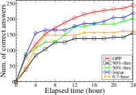
(a) Additive utility: Num. of all typo corrections by workers

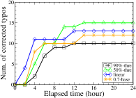
(b) Non-additive utility: Num. of corrected typos

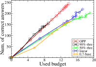
(c) Additive utility with respect to used budget

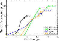
(d) Non-additive utility with respect to used budget

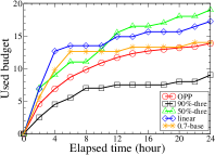
(e) Used budget

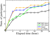
(f) Num. of participants

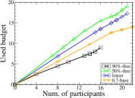
(g) Used budget by Num. of participants

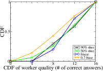
(h) CDF of worker quality (# of correct answers)

Figure 3: Experimental results of a typo correction task in Amazon Mechanical Turk over $24$ hours with various pricing policies. In (b), a typo is regarded as being corrected, if corrected by at least $8$ workers.

5.2 Evaluation

Efficiency of common pricing

Figure 3LABEL:sub@fig:exp-util shows the accumulated number of typo corrections, corresponding to an additive utility. In Figure 3LABEL:sub@fig:exp-util, we observe that the common pricing $50\%$-thre and linear nearly achieves up to $83\%$ and $91\%$ of the utility of OPP at $t=24$, respectively. Figure 3LABEL:sub@fig:exp-budget represents the budget consumption of policies with respect to elapsed time. We observe that the total budget consumption for $50\%$-thre and linear are just about $1.4$ and $1.3$ times more than that of OPP. Combining these two results, we verify that with small additional budget in common pricing with bonus policy, their achieved utility is close to that of OPP. Moreover, we note that the simulated OPP is designed to underestimate the overall cost distribution of workers, because any workers with cost lower than $0.7$ will accept the $0.7$-base policy, but we just assume that their is $0.7$. It implies a smaller gap between $50\%$-thre and linear and the real OPP.

Power of bonus

In Figures 3LABEL:sub@fig:exp-util-3LABEL:sub@fig:exp-budget, employing bonus significantly helps to improve the utility or save the budget spent. For example, $0.7$-base spent almost $2$ times more budget than $90\%$-thre, but they collect a similar number of typo corrections at the end. This means that the bonus payment can double the ratio of utility to budget. This supports the non-negligible power of bonus as analyzed in Theorem 3, where bonus payment incentivizes high quality workers and increases the efficiency of budget usage. Indeed, in Figure 3LABEL:sub@fig:cdf-worker, the pricing without bonus, e.g., $0.7$-base, shows to be the most skewed distribution towards poor workers due to the lack of incentive for quality workers.

Structure of utility and bonus

We now study the impact of the form of utility function and bonus. In Figure 3LABEL:sub@fig:exp-util, we observe that linear eventually achieves the highest utility among all the common pricing policies, and also the highest final utility-to-budget ratio in Figure 3c. For additive U1, to achieve high utility, the requester has to maximize $\sum_{i}s_{i}/B\sim\sum_{i}s_{i}/\sum_{i}c_{i}$. Hence the requester naturally needs to maximize $s_{i}/c_{i}$ for each worker $i$, and we find that linear naturally achieves this behavior, since it only recruits workers with $s_{i}/c_{i}$ larger than or equal to a specific threshold. Therefore, if the requester wants to maximize an additive utility, (e.g., findings many as possible typos in the typo-correction task), linear would be a proper answer. Next, for a non-additive U2 in Figure 3LABEL:sub@fig:apd_utility, we observe that $50\%$-thre achieves the highest utility, and the highest final utility-to-budget ratio in Figure 3LABEL:sub@fig:exp-uAToB-nonsep. In this case, maximizing per-worker contribution-to-cost ratio does not necessarily optimize the utility. Hence, if the requester decides to trust the corrected typo, if at least $n_{\text{cor}}$ workers give the same answer, she needs to exploit $m\%$-thre. However, we also find that if the bonus granting condition is too cruel as in $90\%$-thre, the requester fails to exhaust given budget with $n$ workers (or within a fixed time), which leads to low utility as seen in Figures 3LABEL:sub@fig:exp-util and LABEL:sub@fig:apd_utility. We find that if the bonus granting condition is too critical, it could happen that no one is possible to earn the bonus regardless of the bonus amount, and hence only the base payment motivates the workers in this case. This “extreme” bonus policy will help more when the requester has enough time, or equivalently has large pool of workers, but experience lack of budget, as we observe that the ratio of U1 (or U2) to consumed budget is the largest in $90\%$-thre.

6 Conclusion

In this paper, we analytically studied the impact of personalization and bonus payment in posted pricing. We prove that a common pricing policy equipped with proper bonus nicely approximates the optimal personalized pricing, where bonus is inevitable for common pricing policy to work well. Our analytical findings, verified through simulations and real experiments, explain why many current crowdsourcing systems work well with simple pricing policies, and present some practical implications on how to price workers better with a simple mechanism according to the characteristic of the crowdsourcing tasks. In what follows, we discuss few future research directions regarding possible irrational behaviors of workers in practice.

Prospect theory

In our model, we assume that each worker $i$ knows the exact value of quality $s_{i}$ and cost $c_{i}$, and computes the best response. However, in practice, there can be some uncertainty in the self-evaluation and expected utility, and this makes worker behavior can be more complex than what we assume. In particular, once we introduce such an uncertainty, we may need to consider risk-averse or risk-seeking behaviors in the literature of prospect theory [KT13], while workers in our model are basically assumed to be risk-neutral. Indeed, the risk-averse behavior is partially observed in our experiment observing the less number of participants recruited by risky pricing (such as $50\%$-thre or $90\%$-thre) than that by safe pricing (such as linear or $0.7$-base) in Figure 3LABEL:sub@fig:num-worker, although our model can also explain this as well. In this sense, we believe that our empirical results might be utilized to reverse-engineer the crowdsourcing worker’s utility in such platform in the context of behavioral game theory [Cam11, Cra97]. After all, since the risk-averse or risk-seeking natures are essentially irrational behavior of workers, we believe the power of bonus in practice is greater than what we studied in this work assuming risk-neutral workers, while we need careful analysis and experiment to compare personalized and common pricings.

Assessing quality of contribution

Our study suggests quality-based pricing for efficiency. Thanks to an extensive line of work [DS79, RYZ⁺10, OOJ⁺19, OOSY16, KOS14], there are a number of off-the-shelf algorithms for worker assessment. However, they could be erroneous in some scenarios. Imprecise worker assessment might discourage the worker’s participation, especially those who tend to avoid a large variability in their reward. This might require us to construct more robust common pricing policy to encourage the participation of such workers. Besides, there might be a strategic tendency to collude for the workers if their contribution is estimated based on the other’s contribution in collective manner. In this context, one might seek to design a pricing policy along with truthful quality assessment process by integrating the concept of proper scoring rule in information elicitation literature [HFC16, LC16, RFJ16, CSZ20]. Nonetheless, we believe that the workers in microtask crowdsourcing platform tends to truthfully report their belief for the most tasks since the tasks are usually simple and easy so that each worker would think that the correctly submitted answers will be majority.

Mechanism complexity

Posted price mechanism indeed simplifies the communication between the requester and workers, and encourages the participation of volatil workers. However, quality-based pricing introduces additional complexity in the worker’s point of view, since each worker needs to estimate own quality in advance to determine whether or not to accept the task by quantifying the expected amount of reward. Since it might discourage the volatile workers’ participation, this is indeed an important factor which requires further study. As an evidence, one can interpret that in Figure 3LABEL:sub@fig:num-worker, linear and $0.7$-base engaged more participants than $50\%$-thre and $90\%$-thre due to their relative simplicity. In this regard, we might consider such mechanism complexity as an additional variable in our optimization problem, whether as an objective or constraint. The line of works studying the menu-size complexity of auction mechanism [BGN21, CTT20, CDO⁺15] could be a guide for such extension. We however note that all the bonus payment schemes which we consider in this paper are much simpler than auction-based ones, e.g., [EFLS18].

Appendix A Experimental detail

We briefly present how we design our Mturk experiment to fairly compare the various pricing schemes. To evenly allocate workers to various pricing schemes, we firstly post a preliminary task at $\$0.02$ to recruit the workers in advance. In the task, we require the workers to agree on receiving an e-mail which asks the workers to participate on a further main task at a specified time. As presented in Figure 4LABEL:sub@fig:pre_test, we attach an illustrative example for the main task, and the workers are committed to type ”YES”. This process enables us to recruit $520$ workers within two days, and we randomly distribute them to each experimental group equipped with corresponding pricing scheme. Each group is finally offered to participate on our main task as described in Figure 4LABEL:sub@fig:e_mail, where the provided pricing contract differs across the groups. We believe that we encourage their strategic decision by explicitly specifying that the task is optional and there would be no further disadvantage in not completing the main task.

In the main task, the workers are requested to find and correct typos as we briefly discussed. The typos are almost evenly distributed over the article, and for each target word, we alter it into an elementary level of typo so that there exists no fundamental difficulty in correcting the typos whenever each worker discovers it. When posting the task in Mturk, we intentionally coat dashed lines in the display of the article in order to prevent the workers to exploit some automated tools, like OCR, which might enable them to solve the task without exerting their own effort. To choose a proper price for our task, we presume that the most workers would spend about $5$ to $10$ minutes in completing the task, and decide the base and bonus payment so that the expected payment divided by spent time stays near in statutory minimum wages.

We now provide the details of how we model and compute the performance of OPP in approximate manner, which we presented as simulated OPP in Section 5. We first assume that the workers are sampled from i.i.d. joint distribution where $c_{i}\sim\text{Uniform}(\{0.1,0.2,\ldots,2.0\})$ and $s_{i}\sim\mathcal{N}(xc_{i}+y,z^{2})$, and they arrive with geometric distribution $G(\lambda)$ for some hidden parameters $x,y,z,\lambda>0$. To infer $x$ and $y$, we compute expected quality for every $b$-base policy where $b\in\{0.1,0.3,0.5,0.7\}$, and then use linear regression over $b$ and expected quality, which leads us to obtain $x=2,y=7,$ by assuming $b=c_{i}$. We obtain $z=4$ by computing the expectation of standard deviation for every $b$-base policy. Finally, we get $\lambda=0.13$ by computing expected arrival interval between any two consecutive workers for every $b$-base policy. Given this model, we first assume that the total budget $B$ is $14$ as in the total consumed budget in $0.7$-base policy. Then, we sample $65$ data from the profile distribution and their arrival time from arrival model, and compute utility at each time of OPP computed from this sample. Finally, we repeat this process 100 times to estimate an expected performance over worker profile and arrival samples.

(a)

(b)

Figure 4: (a) The actual pre-task display used in the experiment (b) The e-mail which was used to provide main task

Appendix B Proof of Main Results

B.1 Proof of Theorems

Proof of Theorem 1

To prove, we consider deterministic worker profiles, i.e., $\mathbb{P}[({s}_{i},{c}_{i})=(\bar{s}_{i},\bar{c}_{i})~{}\forall i\in\mathcal{N}]~{}=~{}1$ for some $[(\bar{s}_{i},\bar{c}_{i})]$. Since it is a special case of our problem, it is sufficient to show that OPP is NP-hard even on this simple setup. Consider the following generalized 0-1 knapsack problem (GKP): for $\bm{s},\bm{c}\in\mathbb{R}^{n}_{\geq 0}$,

$$\text{\bf GKP:}\quad\underset{\bm{x}\in\{0,1\}^{n}}{\textnormal{maximize}} \quad u(\bm{{s}}\circ\bm{x})$$

subject to $$\quad\sum_{i=1}^{n}{c}_{i}x_{i}\leq B\;.$$ (6a)

It is well-known that GKP with an additive $u(\cdot)$ is NP-hard [Dan57]. We now show that (i) if $[p_{i}^{\star}]$ is a solution of OPP in (4), then a solution of GKP in (6) is given as $[(\phi_{i}(p^{\star}_{i})\})]$ in (1), and (ii) if $[(x_{i}^{\star})]$ is a solution of GKP, then a solution of OPP is given as $p_{i}=c_{i}\cdot x_{i}.$ We prove (i) and (ii) by contradiction.

(i). Let $\bm{x}^{\star}=\{\phi_{i}(p_{i}^{\star})\}_{i\in\mathcal{N}}$, where $p^{\star}=\{p_{i}^{\star}\}_{i\in\mathcal{N}}$ is the solution of OPP, i.e., utility of $p^{\star}$ is $u(\bm{s}\circ\bm{x}^{\star})$. Then it is straightforward to check that $\bm{x}^{\star}$ satisfies the constraint in (6a). Suppose $\bm{x}^{\star}$ is not a solution of GKP so that there exists a solution $\bm{x}^{\prime}$ such that $u(\bm{s}\circ\bm{x}^{\prime})>u(\bm{s}\circ\bm{x}^{\star})$. We now construct a personalized pricing $\pi^{\prime}=\{c_{i}x^{\prime}_{i}\}_{i\in\mathcal{N}}$ from $\bm{x}^{\prime}$. Since $\bm{x}^{\prime}$ is a solution of GKP, pricing $\pi^{\prime}$ satisfies the constraints in (2). The construction of ${\pi}^{\prime}$ contradicts the optimality of $\pi^{\star},$ since the utility of $\pi^{\prime}$ is strictly larger than that of $\pi^{\star}$.

(ii). Let $[(x_{i}^{\star})]$ be an optimal solution of GKP. Let $[p_{i}]$ be a solution of OPP such that $u(\bm{s}\circ[p_{i}])>u(\bm{x}\circ\bm{x}^{\star})$. We now construct an allocation vector $x^{\prime}=[(\mathbbm{1}[p_{i}(s_{i})\geq c_{i}])]$ from personalized pricing $[p_{i}]$. Since $[p_{i}]$ is budget-feasible, it is straightforward that $x^{\prime}$ is a feasible solution of GKP, which again contradicts the optimality of $[(x^{\star})]$, and it completes the proof. $\Box$

Proof of Theorem 2

We first lay out the foundations in defining the ex-ante budget constraint as follows: For $B\geq 0$ and $\pi\in\mathcal{F}(B):=\{\pi:\sum_{i\in\mathcal{N}}\mathbb{E}[(p_{i}(s_{i})\mathbbm{1}[p_{i}(s_{i})>c_{i}]]\leq B\}$, let $\mathcal{Q}(p,B)$ be the distribution of random vector $\bm{y}\in\{0,1\}^{\mathcal{N}}$ consisting of $y_{i}=\max\big{\{}\mathbbm{1}[p_{i}(s_{i})>c_{i}],\mathbbm{1}[p_{i}(s_{i})=c_{i}]b_{i}\big{\}}.$ Here, $b_{i}$ is an independent Bernoulli random variable with parameter $\rho(\pi,B)$, where

$$\rho(\pi,B):=\min\left\{1,\frac{B-\sum_{i\in{\mathcal{N}}}\mathbb{E}[(p_{i}(s_{i}))\mathbbm{1}[p_{i}(s_{i})>c_{i}]]}{\sum_{i\in{\mathcal{N}}}\mathbb{E}[(p_{i}(s_{i}))\mathbbm{1}[p_{i}(s_{i})=c_{i}]]}\right\}\;.$$

Note that $\rho(p,B)\geq 0$ directly comes from the definition of $\pi$.

Thanks to the generation of $\bm{y}\sim\mathcal{Q}(\pi,B)$ and condition on $\pi\in\mathcal{F}(B)$, the task allocation according to $\bm{y}$ verifies budget constraint in expectation sense:

$$\textstyle\mathbb{E}_{\bm{y}\sim\mathcal{Q}(p,B)}\big{[}\sum_{i\in\mathcal{N}}(p_{i}(s_{i}))y_{i}\big{]}\leq B,$$

which is also known as ex-ante budget constraint. We then formulate an ex-ante version of OPP$(B)$ in (4) as follows:

$$\text{ {\bf OPP-E}$(B)$:}\quad\underset{p\in\mathcal{F}(B)}{\textnormal{maximize}} \quad V(B;p)$$ (7)

where $V(B;p):=\mathbb{E}_{\bm{y}\sim\mathcal{Q}(p,B)}[U(\bm{s}\circ\bm{y})]$.

We consider a common pricing that has linear bonus with zero base payment, which we call LBZB pricing and denote by $p_{c}(\alpha)$ with the slope $\alpha\geq 0$, i.e., $p_{c}(\alpha):=\alpha s$. Next we define a constant $\alpha_{B}$ as the following:

$$\alpha_{B}\mathrel{:=}\inf\left\{\alpha\geq 0:\sum_{i\in\mathcal{N}}\mathbb{E}\big{[}c_{i}z_{i}(\alpha,\lambda)\big{]}\geq B,~{}\exists\lambda\in[0,1]\right\},$$

for a random variable $z_{i}$ defined as $z_{i}(\alpha,\lambda)\mathrel{:=}\mathbbm{1}[\alpha s_{i}>c_{i}]+\lambda\mathbbm{1}[\alpha s_{i}=c_{i}].$ Now we prove that $p_{c}(\alpha_{B})$ achieves the approximation ratio stated in the theorem.

We present two key lemmas whose proofs are in Section B.2.

Lemma 1 (Ex-ante PoA).

LBZB pricing $p_{c}$$(\alpha_{B})$ is $(1,\mu_{B})$-approximate of $\text{OPP-E}(B)$, where $\mu_{B}$ is defined as follows:

$$\mu_{B}\mathrel{:=}\frac{\sum_{i\in\mathcal{N}}\mathbb{E}\big{[}\alpha_{B}s_{i}z_{i}(\alpha_{B},\lambda_{B})\big{]}}{\sum_{i\in\mathcal{N}}\mathbb{E}[c_{i}z_{i}(\alpha_{B},\lambda_{B})]},\quad\text{where}$$

$$\lambda_{B}\mathrel{:=}\inf\left\{\lambda\in[0,1]:\sum_{i\in\mathcal{N}}\mathbb{E}\big{[}c_{i}z_{i}(\alpha_{B},\lambda)\big{]}\geq B\right\}.$$

Lemma 2 (Connection to ex-post).

For any $k=\omega(1)$ and $\varepsilon=o(1)$ with $k\varepsilon>2$, we have

$$U\!\Big{(}\mu_{B}B;p_{c}(\alpha_{B})\Big{)}\geq\Big{(}1-e^{-\varepsilon^{2}(1-\varepsilon)k/12}\Big{)}V\!\Big{(}\mu_{B}B;p_{c}(\alpha_{B})\Big{)}.$$

Lemma 1 provides an approximation ratio of $p_{c}(\alpha_{B})$ to OPP-E$(B)$. We then use Lemma 2 with $k=n^{1/2}$ and $\varepsilon=n^{-1/6}$ to translate the ex-ante approximation into the ex-post one, where we have

$$U\!\Big{(}\mu_{B}B;p_{c}(\alpha_{B})\Big{)} \geq\Big{(}1-O(e^{-n^{1/6}})\Big{)}V\!\Big{(}\mu_{B}B;p_{c}(\alpha_{B})\Big{)}\geq\Big{(}1-O(e^{-n^{1/6}})\Big{)}V^{\star}(B).$$

This concludes the proof since $V^{\star}(B)\geq U\big{(}B;\pi^{\star}_{p}(B)\big{)}$ and $\mu_{B}=O(1)$ by assumption. $\Box$

Observation on LBZB

We provide a couple of interpretations of LBZB introduced in the proof of Theorem 2. We note that the linear bonus in the LBZB pricing $p_{c}(\alpha)$ recruits only efficient workers whose utility-to-cost ratio $s_{i}/c_{i}$ is at least $1/\alpha$, i.e., $x_{i}=1$ only if $s_{i}/c_{i}\geq{1}/{\alpha}$. A good personalized pricing may also target such efficient workers in priority, while user-agnosticism of the common pricing pays more often than the personalized one. Hence, the simple common pricing $p_{c}(\alpha)$ with a good choice of $\alpha=\alpha_{B}$ and more budget $(O(1)\times B)$ achieves at least $1-o(1)$ of the optimal utility of OPP$(B)$.

We also note that one can get tighter bound on utility by optimizing the parameters in Lemma 2, we instead use a naive parameter just to show the insight that LBZB achieves asymptotically optimal utility within constant amount of augmented budget.

For the employed LBZB common pricing to be practical, it is required that $\alpha_{B}$ allows easy computation, which turns to be polynomial-time computable with respect $n$ in approximate manner. To do so, given all the distributions of worker profiles, it is enough to find $\alpha$ such that $\sum_{i\in\mathcal{N}}\mathbb{E}\big{[}c_{i}\mathbbm{1}[\alpha s_{i}\geq c_{i}]\big{]}\geq B$ and $\sum_{i\in\mathcal{N}}\mathbb{E}\big{[}c_{i}\mathbbm{1}[\alpha s_{i}>c_{i}]\big{]}\leq B$, where of each term in the summations can be computed in $O(1)$ time. Since the available interval of $\alpha$ is bounded, using some root finding algorithms, we can find such $\alpha$ approximately in at most $c\cdot O(1)\cdot 2n$ time for some constant $c$.

Proof of Theorem 3

For a given budget $B$, we denote $u^{\star}(B)$ and $u_{0}^{\star}(B)$ to be the utilities of an optimal pricing by solving $\text{OPP}(B)$, and an optimal common pricing without bonus, respectively. Given a budget $B$, we also can find $c_{0}$ such that $c_{0}n>B$. Now, for $\varepsilon=\frac{B}{n^{2}c}<1$, consider the following profiles of $n$ workers:

$$(s_{i},c_{i})= (s_{0},c_{0}) 0<i\leq\varepsilon n$$ if

$$(s_{i},c_{i})= (0,c_{0}) \varepsilon n<i\leq n$$ if .

For simplicity, we assume that $\varepsilon n$ is an integer without loss of generality. Then, it is straightforward to check that $u^{\star}(B)=\varepsilon ns$. Now we compute the optimal utility for pricing without personalization nor bonus under the worst-case worker arrival model. Consider a scenario where all the spammers arrive ahead of the hammers. We assume that the budget is augmented by a factor $\delta=o(n)$. Then, the total payment to spammers is computed as the following:

$$(1-\varepsilon)cn=nc-B/n\geq\delta B,$$

where the inequality comes from that $\delta=o(n)$. Hence, the optimal common pricing without bonus failed to recruit any hammers, and it concludes the proof. $\Box$

B.2 Proof of Lemmas

Proof of Lemma 1

We prove that $V(\mu_{B}B;p_{c}(\alpha_{B}))$ exactly achieves the optimum of ex-ante mechanism given budget $B$, i.e., $V(\mu_{B}B;p_{c}(\alpha_{B}))\geq V^{\star}(B)$. First, since $s_{i}/c_{i}$ is also a positive random variable, it is straightforward to have that the right-continuity of CDF of $s_{i}/c_{i}$ implies that $\mathbb{E}[c_{i}z_{i}(\alpha_{B},\lambda_{B})]=B$. We now consider the following relaxed version of the ex-ante mechanism.

$$\text{ {\bf Oracle}$(B)$:}\quad\underset{\bm{x}=[(x_{i}(s_{i},c_{i}))]\in[0,1]^{n}}{\textnormal{maximize}} \quad\sum_{i\in\mathcal{N}}\mathbb{E}\left[u(s\circ x))\right]$$

s.t. $$\quad\sum_{i\in\mathcal{N}}\mathbb{E}\left[c_{i}x_{i}\right]\leq B.$$

Note that $\bm{x}$ is not necessarily sampled from $\mathcal{Q}(\bm{\pi},B)$, so that the domain of $\bm{x}$ is also extended to any real number in $[0,1]^{n}$. It is trivial that the optimum of Oracle($B$) is dominant to that of ex-ante mechanism given budget $B$. We show that the allocation vector obtained by common pricing $p_{c}(\alpha_{B})$ under ex-ante mechanism becomes optimal for Oracle($B$). We first introduce two lemmas that are useful in the proof whose proofs are presented in the end of this section.

Lemma 3.

Let $\bm{z}^{\star}$ be any optimal allocation vector for Oracle($B$). The following holds for any random incidence of random vector $(\bm{s},\bm{c})$.

1. If $\alpha_{B}s_{i}<c_{i}$, then $z_{i}^{\star}(s_{i},c_{i})=0$ a.e. for any $i\in\mathcal{N}$.

2. If $\alpha_{B}s_{i}>c_{i}$, then $z_{i}^{\star}(s_{i},c_{i})=1$ a.e. for any $i\in\mathcal{N}$.

Lemma 4.

For $i\in\mathcal{N},$ let $\mathcal{H}_{i}=\left\{(s_{i},c_{i})|\alpha_{B}s_{i}=c_{i}\right\}$. Let $\bm{x}$ and $\bm{x}^{\prime}$ be the two random allocation vectors which satisfies $\sum_{i\in\mathcal{N}}\mathbb{E}_{(s_{i},c_{i})\in\mathcal{H}_{i}}[c_{i}x_{i}]\geq(=)\sum_{i\in\mathcal{N}}\mathbb{E}_{(s_{i},c_{i})\in\mathcal{H}_{i}}[c_{i}x_{i}^{\prime}].$ Then, the expected utility of $\bm{x}$ is at least that of $\bm{x}^{\prime}$ under $\mathcal{H}_{i}$, i.e.,

$$\sum_{i\in\mathcal{N}}\mathbb{E}_{(s_{i},c_{i})\in\mathcal{H}_{i}}[s_{)}x_{i}]\geq(=)\sum_{i\in\mathcal{N}}\mathbb{E}_{(s_{i},c_{i})\in\mathcal{H}_{i}}[s_{i}x_{i}^{\prime}].$$

Let $\bm{\chi}$ be the allocation vector induced by $p_{c}(\alpha_{B})$ under the augmented budget $\mu_{B}B$. By Lemma 3, it is straightforward to check that optimal allocation vector $\bm{z}^{\star}$ must recruit worker $i$ if $\alpha_{B}s_{i}>c_{i}$, and must reject her if $\alpha_{B}s_{i}<c_{i}$. We first consider the scenario where only allocating the budget to workers with $\alpha_{B}s_{i}>c_{i}$ fully exhaust the budget $B$. In this case, $\sum_{i\in\mathcal{N}}\mathbb{E}[c_{i}z_{i}^{\star}\mathbbm{1}[\alpha_{B}s_{i}>c_{i}]]=B$, and it implies that $\bm{\chi}$ is exactly the same as $\bm{z}$ by the definition of $\alpha_{B}$. Moreover, the expected payment to workers in $p_{c}(\alpha_{B})$ can be computed as:

$$\sum_{i\in\mathcal{N}}\mathbb{E}[\alpha_{B}s_{i}z_{i}(\alpha_{B},\lambda_{B})]=\sum_{i\in\mathcal{N}}\mathbb{E}\Bigl{[}\alpha_{B}s_{i}\mathbbm{1}[\alpha_{B}s_{i}>c_{i}]\Bigr{]}=\mu_{B}B,$$

which guarantees that $p_{c}(\alpha_{B})$ is $\mu_{B}B$-budget feasible, and concludes the proof. We now suppose that the budget is not exhausted, hence optimal allocation vector must recruit some workers with $\alpha_{B}s_{i}=c_{i}$ (workers at boundary), i.e., $\sum_{i\in\mathcal{N}}\mathbb{E}[c_{i}z_{i}^{\star}\mathbbm{1}[\alpha_{B}s_{i}>c_{i}]]<B$. By the definition of $\alpha_{B}$ and $\lambda_{B}$, the following holds:

$$\sum_{i\in\mathcal{N}}\mathbb{E}[c_{i}\chi_{i}\mathbbm{1}[\alpha_{B}s_{i}=c_{i}]] =\sum_{i\in\mathcal{N}}\mathbb{E}[c_{i}\mathbbm{1}[\alpha_{B}s_{i}=c_{i}]]\cdot\rho(p_{c}(\alpha_{B}),\mu_{B}B)$$ (9)

$$=\sum_{i\in\mathcal{N}}\mathbb{E}[c_{i}\mathbbm{1}[\alpha_{B}s_{i}=c_{i}]]\cdot\frac{\mu_{B}B-\sum_{i\in\mathcal{N}}\mathbb{E}[\alpha_{B}s_{i}\mathbbm{1}[\alpha_{B}s_{i}>c_{i}]]}{\sum_{i\in\mathcal{N}}\mathbb{E}[\alpha_{B}s_{i}\mathbbm{1}[\alpha_{B}s_{i}=c_{i}]]}$$ (10)

$$=\mu_{B}B-\sum_{i\in\mathcal{N}}\mathbb{E}[\alpha_{B}s_{i}\mathbbm{1}[\alpha_{B}s_{i}>c_{i}]].$$ (11)

Moreover, it is straightforward to see that any optimal allocation vector $z^{\star}$ must exhaust the budget in workers with $\alpha_{B}s_{i}=c_{i}$, i.e.,

$$\sum_{i\in\mathcal{N}}\mathbb{E}[c_{i}z_{i}^{\star}\mathbbm{1}[\alpha_{B}s_{i}=c_{i}]]=B-\sum_{i\in\mathcal{N}}\mathbb{E}[c_{i}z_{i}^{\star}\mathbbm{1}[\alpha_{B}s_{i}>c_{i}]].$$ (12)

Now we show that the cost consumed by $\bm{\chi}$ is bigger than or equal to that by $\bm{z^{\star}}$. For notational simplicity, we define the random variables $\mathbbm{1}[\alpha_{B}s_{i}>c_{i}]$ and $\mathbbm{1}[\alpha_{B}s_{i}=c_{i}]$ to be $L_{i}$ and $E_{i}$, respectively, and $\rho(p_{c}(\alpha_{B}),\mu_{B}B)$ to be $\rho_{0}$. From equation (11),

$$\mu_{B}B-\sum_{i\in\mathcal{N}}\mathbb{E}[\alpha_{B}s_{i}L_{i}] =\mu_{B}B-\sum_{i\in\mathcal{N}}\mathbb{E}[\alpha_{B}s_{i}L_{i}]-\sum_{i\in\mathcal{N}}\mathbb{E}[\alpha_{B}s_{i}E_{i}]\rho_{0}+\sum_{i\in\mathcal{N}}\mathbb{E}[\alpha_{B}s_{i}E_{i}]\rho_{0}$$ (13)

$$=\mu_{B}B-\mu_{B}(\sum_{i\in\mathcal{N}}\mathbb{E}[c_{i}L_{i}]+\sum\mathbb{E}[c_{i}E_{i}]\rho_{0})+\sum_{i\in\mathcal{N}}\mathbb{E}[\alpha_{B}s_{i}E_{i}]\rho_{0}$$ (14)

$$=\mu_{B}(B-\sum_{i\in\mathcal{N}}\mathbb{E}[c_{i}L_{i}])+\sum_{i\in\mathcal{N}}\mathbb{E}[\alpha_{B}s_{i}E_{i}]\rho_{0}-\mu_{B}\sum_{i\in\mathcal{N}}\mathbb{E}[c_{i}E_{i}]\rho_{0}$$ (15)

$$=\mu_{B}(B-\sum_{i\in\mathcal{N}}\mathbb{E}[c_{i}L_{i}])-\sum_{i\in\mathcal{N}}\mathbb{E}[c_{i}E_{i}]\rho_{0}(\mu_{B}-1)$$ (16)

$$\geq B-\sum_{i\in\mathcal{N}}\mathbb{E}[c_{i}L_{i}],$$ (17)

which is the RHS of equation (12), i.e. the expected payment in random allocation vector $\bm{z}^{\star}$. Note that equation (14) holds from the definition of $\mu_{B}$, equation (16) holds since $\alpha_{B}s_{i}=c_{i}$ under the regime that $E_{i}=1$, and inequality (17) holds from the fact that $\sum_{i\in\mathcal{N}}\mathbb{E}[c_{i}(L_{i}+\rho_{0}E_{i})]\leq\sum_{i\in\mathcal{N}}\mathbb{E}[\alpha_{B}s_{i}(L_{i}+\rho_{0}E_{i})]\leq B$. Finally by Lemma 4, we have:

$$\sum_{i\in\mathcal{N}}\mathbb{E}_{(s_{i},c_{i})\in H_{i}}[s_{i}\chi_{i}]\geq\sum_{i\in\mathcal{N}}\mathbb{E}_{(s_{i},c_{i})\in H_{i}}[s_{i}z_{i}^{\star}],$$ (18)

which implies that the expected utility gain from workers at boundaries, i.e. workers satisfying $\alpha_{B}s_{i}=c_{i}$, is larger or equal on $\bm{\chi}$ than $\bm{z^{\star}}$. Since it is obvious that $p_{c}(\alpha_{B})$ is $\mu_{B}B$-budget feasible, combining Lemma 3 and (18), we complete the proof of Lemma 1. $\Box$

Proof of Lemma 2

For simplicity, we denote LBZB pricing $p_{c}(\alpha_{B})$ by $q$. Let $P$ be a random variable defined by $P=\sum_{i\in\mathcal{N}}q(s_{i})$. Now we prove that tail probability that the sum of payments to workers $P$ is larger than $(1-1/k)\mu_{B}B$, is lowered bounded by some exponent on $\varepsilon$ and $k$. Since $\varepsilon=o(1)$, $\mu_{B}=O(1)$, and payment to any worker on LBZB is bounded above by constant asymptotically, we have $\mathbb{E}[P]\leq(1-\varepsilon)\mu_{B}B$ for sufficiently large $n$. Without loss of generality, we can in fact assume that $\mathbb{E}[P]=(1-\varepsilon)\mu_{B}B$ by adding some dummy base payment since it can only increase the right tailed probability. Since $k\varepsilon>2$, we have the following inequalities:

$$\mathbb{P}[P\geq(1+\frac{\varepsilon}{2})\mathbb{E}[P]]=\mathbb{P}[P\geq(1+\frac{\varepsilon}{2})(1-\varepsilon)B] \geq\mathbb{P}[P>(1-\frac{\varepsilon}{2})\mu_{B}B]$$ (19)

$$\geq\mathbb{P}[P>(1-1/k)\mu_{B}B].$$ (20)

Now we define $Y_{i}=\frac{q(s_{i})k}{\mu_{B}B}$ and $Y=\sum_{i\in\mathcal{N}}Y_{i}$. Since $k=\omega(1)$, one can easily get $Y_{i}\in[0,1]$ for sufficiently large $n$, where we have the following inequality:

$$\mathbb{P}[P\geq(1+\frac{\varepsilon}{2})\mathbb{E}[P]] =\mathbb{P}[P\frac{k}{\mu_{B}B}\geq\frac{k}{\mu_{B}B}(1+\frac{\varepsilon}{2})\mathbb{E}[P]]=\mathbb{P}[Y\geq(1+\frac{\varepsilon}{2})\mathbb{E}[Y]]$$ (21)

$$\leq\exp(-\frac{\varepsilon^{2}/4}{2+\varepsilon/2}\cdot\mathbb{E}[Y])=\exp(-\frac{\varepsilon^{2}/4}{2+\varepsilon/2}\cdot\frac{k}{\mu_{B}B}\mathbb{E}[P])$$ (22)

$$=\exp(-\frac{\varepsilon^{2}/4}{2+\varepsilon/2}\cdot\frac{k}{\mu_{B}B}(1-\varepsilon)\mu_{B}B)\leq\exp(-\frac{\varepsilon^{2}(1-\varepsilon)k}{12}).$$ (23)

Inequality in (22) follows from Chernoff bound and (23) follows from $\varepsilon\leq 1$. Hence by (20) and (23), we have the following inequality:

$$\mathbb{P}[P\leq(1-1/k)\mu_{B}B]\geq 1-\exp(-\varepsilon^{2}(1-\varepsilon)k/12).$$ (24)

Next, in ex-post mechanism with augmented budget $\mu_{B}B$, we claim that the probability that any worker is offered the pricing policy (not discarded by the ex-post budget constraint) is at least $\mathbb{P}[P\leq(1-1/k)\mu_{B}B]$, i.e. the probability that the sum of the payments to all the workers is at most $(1-1/k)\mu_{B}B$. This is quite obvious since if the sum of payments to all the workers is at most $(1-1/k)\mu_{B}B$ for any random incidence, then the budget remains in this moment and any worker will be offered the pricing policy. Hence, we have the following inequalities on the expected utility of LBZB in ex-post mechanism:

$$U(\mu_{B}B;p_{c}(\alpha_{B})) =\mathbb{E}_{\bm{x}\sim\mathcal{P}(p_{c}(\alpha_{B}),B,\sigma)}[u(\bm{s}\circ\bm{x})]$$ (25)

$$\geq\sum_{i\in\mathcal{N}}\mathbb{E}\Bigl{[}s_{i}\cdot z_{i}(\alpha_{B},\lambda_{B})\Bigr{]}\mathbb{P}[P\leq(1-1/k)B]$$ (26)

$$\geq\sum_{i\in\mathcal{N}}\mathbb{E}\Bigl{[}s_{i}\cdot z_{i}(\alpha_{B},\lambda_{B})\Bigr{]}\left(1-\exp(-\varepsilon^{2}(1-\varepsilon)k/12)\right)$$ (27)

$$=\left(1-\exp(-\varepsilon^{2}(1-\varepsilon)k/12)\right)V(\mu_{B}B;p_{c}(\alpha_{B})),$$ (28)

and it concludes the proof. $\Box$

Proof of Lemma 3

The underlying intuition is that greedy algorithm outputs the exact optimum of the fractional knapsack problem. We use proof by contradiction. Let the sample space of the random vector $(s_{i},c_{i})$ be $O_{i}$. We define the following sets.

$$\mathcal{E}_{i} :=\{(\bm{s},\bm{c})\;|\;\alpha_{B}s_{i}<c_{i},z_{i}^{\star}(\bm{s},\bm{c})>0\}$$

$$\mathcal{F}_{i} :=\{(\bm{s},\bm{c})\;|\;\alpha_{B}s_{i}\geq c_{i},z_{i}^{\star}(\bm{s},\bm{c})<1\}$$

$$\mathcal{G}_{i} :=\{(\bm{s},\bm{c})\;|\;\alpha_{B}s_{i}\geq c_{i},z_{i}^{\star}(\bm{s},\bm{c})=1\}.$$

Note that given any optimal allocation vector $z^{\star}(\bm{s},\bm{c})$, $E_{i}$ denotes the set of all incidences of random vector $(\bm{s},\bm{c})$ that satisfies $\alpha_{B}s_{i}<c_{i}$ and $z^{\star}_{i}(\bm{s},\bm{c})>0$. Firstly, we claim that if there exists $i\in\mathcal{N}$ such that $\mathbb{P}\Bigl{[}\mathcal{E}_{i}\Bigr{]}>0,$ then there exist $j\in\mathcal{N}$ such that $\mathbb{P}\Bigl{[}\mathcal{F}_{j}\Bigr{]}>0$. Suppose not, i.e. $\mathbb{P}\Bigl{[}\mathcal{E}_{i}\Bigr{]}>0$ for $i\in\mathcal{N}$, and $\mathbb{P}\Bigl{[}\mathcal{F}_{j}\Bigr{]}=0$ for any $j\in\mathcal{N}$. By assumption, we get $\mathbb{P}\Bigl{[}\mathcal{G}_{j}\Bigr{]}=\mathbb{P}\Bigl{[}\alpha_{B}s_{i}\geq c_{i}\Bigr{]}$. Since $\mathcal{E}_{i}$, $\mathcal{F}_{i}$, and $\mathcal{G}_{i}$ are mutually exclusive, the expected payment to workers in $\bm{z}^{\star}$ satisfies the following inequalities:

$$B \geq\sum_{i\in\mathcal{N}}\mathbb{E}_{(s_{i},c_{i})\in\mathcal{E}_{i}}[c_{i}z_{i}^{\star}]+\mathbb{E}_{(s_{i},c_{i})\in\mathcal{F}_{i}}[c_{i}z_{i}^{\star}]+\mathbb{E}_{(s_{i},c_{i})\in\mathcal{G}_{i}}[c_{i}z_{i}^{\star}]$$ (29)

$$\geq\sum_{i\in\mathcal{N}}\mathbb{E}_{(s_{i},c_{i})\in\mathcal{E}_{i}}[c_{i}z_{i}^{\star}]+\mathbb{E}_{(s_{i},c_{i})\in\mathcal{G}_{i}}[c_{i}z_{i}^{\star}]$$ (30)

$$\geq\sum_{i\in\mathcal{N}}\mathbb{E}_{(s_{i},c_{i})\in\mathcal{E}_{i}}[c_{i}z_{i}^{\star}]+\mathbb{E}[c_{i}\mathbbm{1}[\alpha_{B}s_{i}\geq c_{i}]]$$ (31)

$$\geq\sum_{i\in\mathcal{N}}\mathbb{E}_{(s_{i},c_{i})\in\mathcal{E}_{i}}[c_{i}z_{i}^{\star}]+B>B,$$ (32)

which is a contradiction. Hence we conclude that if there exists $i\in\mathcal{N}$ with $\mathbb{P}\Bigl{[}\mathcal{E}_{i}\Bigr{]}>0,$ then there exists $j\in\mathcal{N}$ with $\mathbb{P}\Bigl{[}\mathcal{F}_{j}\Bigr{]}>0$. By our claim, we can choose two random incidences $(\bar{s_{i}},\bar{c_{i}})\in\mathcal{E}_{i}$ and $(\tilde{s_{j}},\tilde{c_{j}})\in\mathcal{F}_{j}$, which are $i$-th and $j$-th element in incidences of random vector $(\bar{\bm{s}},\bar{\bm{c}})$ and $(\tilde{\bm{s}},\tilde{\bm{c}})$, respectively. Now we construct an allocation vector $\bm{y}\in[0,1]^{n}$, which is equal to $\bm{z}^{\star}$ except the two sample points $(\bar{\bm{s}},\bar{\bm{c}})$ and $(\tilde{\bm{s}},\tilde{\bm{c}})$ so that $y_{j}(\tilde{s_{j}},\tilde{c_{j}})=z_{j}^{\star}(\tilde{s_{j}},\tilde{c_{j}})+\varepsilon$, and $y_{i}(\bar{s_{i}},\bar{c_{i}})=z_{i}^{\star}(\bar{s_{i}},\bar{c_{i}})-\frac{\tilde{c_{j}}}{\bar{c_{i}}}\varepsilon$, where $\varepsilon=\min\left\{\frac{\bar{c_{i}}}{\tilde{c_{j}}}z_{i}^{\star}(\bar{s_{i}},\bar{c_{i}}),1-z_{j}^{\star}(\tilde{s_{j}},\tilde{c_{j}})\right\}$. Then, the difference between the total expected payment to workers in $\bm{y}$ and $\bm{z}^{\star}$ can be computed as the following:

$$\sum_{i\in\mathcal{N}}\mathbb{E}[c_{i}z_{i}^{\star}]-\sum_{i\in\mathcal{N}}\mathbb{E}[c_{i}y_{i}] =\left(\tilde{c_{j}}y_{j}(\tilde{s_{j}},\tilde{c_{j}})+\bar{c_{i}}y_{i}(\bar{s_{i}},\bar{c_{i}})\right)-\left((\tilde{c_{j}}z_{j}^{\star}(\tilde{s_{j}},\tilde{c_{j}})+\bar{c_{i}}z_{i}^{\star}(\bar{s_{i}},\bar{c_{i}}))\right)$$

$$=\tilde{c_{j}}(z_{j}^{\star}(\tilde{s_{j}},\tilde{c_{j}})+\varepsilon)+\bar{c_{i}}(z_{i}^{\star}(\bar{s_{i}},\bar{c_{i}})-\frac{\tilde{c_{j}}}{\bar{c_{i}}}\varepsilon)-(\tilde{c_{j}}z_{j}^{\star}(\tilde{s_{j}},\tilde{c_{j}})+\bar{c_{i}}z_{i}^{\star}(\bar{s_{i}},\bar{c_{i}}))$$

$$=\tilde{c_{j}}\varepsilon-\bar{c_{i}}\cdot\frac{\tilde{c_{j}}}{\bar{c_{i}}}\varepsilon=0,$$

which implies that $\bm{y}$ is also a feasible point for Oracle($B$). Now we compute the difference of expected utility between $\bm{y}$ and $\bm{z}^{\star}$ as the following:

$$\sum_{i\in\mathcal{N}}\mathbb{E}[s_{i}y_{i}]-\sum_{i\in\mathcal{N}}\mathbb{E}[s_{i}z_{i}^{\star}] =\tilde{s_{j}}(z_{j}^{\star}(\tilde{s_{j}},\tilde{c_{j}})+\varepsilon)+\bar{s_{i}}(z_{i}^{\star}(\bar{s_{i}},\bar{c_{i}})-\frac{\tilde{c_{j}}\varepsilon}{\bar{c_{i}}})-\Big{(}\tilde{s_{j}}z_{j}^{\star}(\tilde{s_{j}},\tilde{c_{j}})+\bar{s_{i}}z_{i}^{\star}(\bar{s_{i}},\bar{c_{i}})\Big{)}$$

$$=\tilde{s_{j}}\varepsilon-\bar{s_{i}}\frac{\tilde{c_{j}}}{\bar{c_{i}}}\varepsilon>\frac{\varepsilon}{\alpha_{B}}(\tilde{c_{j}}-\bar{c_{i}}\frac{\bar{c_{i}}}{\bar{c_{i}}})=0,$$

which implies that the expected utility of $\bm{y}$ is strictly larger than $\bm{z}.$ This contradicts the assumption that $\bm{z}$ is optimal solution for Oracle($B$), and it completes the proof of Lemma 4.3. Since the proof for statement (ii) is exactly analogous to that of (i), we omit the detailed proof. $\Box$

Proof of Lemma 4

The following inequality directly completes the proof.

$$\sum_{i\in\mathcal{N}}\mathbb{E}_{(s_{i},c_{i})\in\mathcal{H}_{i}}[s_{i}x_{i}]=\sum_{i\in\mathcal{N}}\mathbb{E}[s_{i}x_{i}\mathbbm{1}[\alpha_{B}s_{i}=c_{i}]] =\sum_{i\in\mathcal{N}}\mathbb{E}\Bigl{[}\frac{c_{i}}{\alpha_{B}}x_{i}\mathbbm{1}[\alpha_{B}s_{i}=c_{i}]\Bigr{]}$$ (33)

$$\geq\sum_{i\in\mathcal{N}}\mathbb{E}\Bigl{[}\frac{c_{i}}{\alpha_{B}}x_{i}^{\prime}\mathbbm{1}[\alpha_{B}s_{i}=c_{i}]\Bigr{]}$$ (34)

$$=\sum_{i\in\mathcal{N}}\mathbb{E}_{(s_{i},c_{i})\in\mathcal{H}_{i}}[s_{i}x_{i}^{\prime}],$$ (35)

where (33) holds from the definition of $\mathcal{H}_{i},$ and (34) and (35) from our assumption. It is also straightforward to check the equality version of the lemma from (34). $\Box$

B.3 Proof of Propositions

Proof of Proposition 1

In ratio-equivalent regime, it is straight forward to check that $\mu_{B}$ introduced in the proof of Lemma 1 is equal to $1$ for $p_{lin}(k)$. Hence from Theorem 2, we conclude that $p_{lin}(k)$ is $(1,1)-$approximate as $n$ goes to infinity. $\Box$

Proof of Proposition 2

In the proof of Theorem 2, we have that $p_{c}(\alpha_{B})$ achieves $(1,\mu_{B})-$approximate in ex-ante version. We now claim that $p_{thre}(c,\beta_{B})$ achieves the same utility approximation ratio without any augmented budget in ex-ante version. By our assumption on cost equivalence, the following holds for the definition of $\alpha_{B}$:

$$\alpha_{B} \mathrel{:=}\inf\left\{\alpha\geq 0:\sum_{i\in\mathcal{N}}\mathbb{E}\big{[}c_{i}z_{i}(\alpha,\lambda)\big{]}\geq B,~{}\exists\lambda\in[0,1]\right\}$$

$$=\inf\left\{\alpha\geq 0:c\sum_{i\in\mathcal{N}}\mathbb{E}\big{[}z_{i}(\alpha,\lambda)\big{]}\geq B,~{}\exists\lambda\in[0,1]\right\}$$

$$=\inf\left\{\alpha\geq 0:c\sum_{i\in\mathcal{N}}\mathbb{P}[\alpha s_{i}\geq c]\geq B\right\}=c\cdot\beta_{B}$$

Hence from Lemma 3, we find that $p_{thre}(c,\beta_{B})$ under ex-ante constraint recruits every workers with $\alpha_{B}s_{i}\geq c_{i}$ as the same as optimal offline algorithm does. Next, the expected payment for the workers at boundary, i.e. workers with $\alpha_{B}s_{i}=c_{i}$, in $p_{thre}(c,\beta_{B})$ under ex-ante constraint is the same as that of optimal offline algorithm as follow:

$$\rho(p_{thre}(c,\beta_{B}),B)\cdot c\sum_{i\in\mathcal{N}}\mathbb{E}[\mathbbm{1}[\alpha_{B}s_{i}=c]] =B-c\sum_{i\in\mathcal{N}}\mathbb{E}[\mathbbm{1}[\alpha_{B}s_{i}>c]]$$

$$=B-\sum_{i\in\mathcal{N}}\mathbb{E}[c_{i}z_{i}^{\star}\mathbbm{1}[\alpha_{B}s_{i}>c_{i}]]$$

$$=\sum_{i\in\mathcal{N}}\mathbb{E}[c_{i}z_{i}^{\star}\mathbbm{1}[\alpha_{B}s_{i}=c_{i}]].$$

Hence by Lemma 4, we find that the expected utility from both $p_{thre}(c,\beta_{B})$ and optimal offline algorithm for the workers at boundary are exactly the same. Finally, $p_{thre}(c,\beta_{B})$ achieves the exact optimum in Oracle problem, and combined with the analogous statement in Lemma 2, $p_{thre}(c,\beta_{B})$ is $(1,1)-$approximate in asymptotic manner. $\Box$

Proof of Proposition 3

Let $p(s_{i})$ be any common pricing equipped with non-zero bonus function. Since the support of $s_{i}$ is a singleton, the support of $p(s_{i})$ for $i\in\mathcal{N}$ is also a singleton, and we let that element be $\nu_{i}$. Then, it is straightforward to check that $p^{\prime}(s_{i})=\nu$ achieves the exact same expected utility as $p(s_{i})$, where it concludes the proof. $\Box$

References

- [AGN14] Nima Anari, Gagan Goel, and Afshin Nikzad. Mechanism design for crowdsourcing: An optimal 1-1/e competitive budget-feasible mechanism for large markets. In Proc. of FOCS, 2014.
- [AKK12] Vineet Abhishek, Ian A Kash, and Peter Key. Fixed and market pricing for cloud services. In 2012 Proceedings IEEE INFOCOM Workshops, pages 157–162. IEEE, 2012.
- [AKS19] Georgios Amanatidis, Pieter Kleer, and Guido Schäfer. Budget-feasible mechanism design for non-monotone submodular objectives: Offline and online. In Proceedings of the 2019 ACM Conference on Economics and Computation, 2019.
- [AS10] Eric T Anderson and Duncan I Simester. Price stickiness and customer antagonism. The quarterly journal of economics, 125(2):729–765, 2010.
- [BBM15] Dirk Bergemann, Benjamin Brooks, and Stephen Morris. The limits of price discrimination. American Economic Review, 105(3):921–57, 2015.
- [BCGL12] Xiaohui Bei, Ning Chen, Nick Gravin, and Pinyan Lu. Budget feasible mechanism design: from prior-free to bayesian. In Proc. of STOC, 2012.
- [BCW19] Dirk Bergemann, Francisco Castro, and Gabriel Weintraub. Third-degree price discrimination versus uniform pricing. arXiv preprint arXiv:1912.05164, 2019.
- [BFN06] Moshe Babaioff, Michal Feldman, and Noam Nisan. Combinatorial agency. In Proceedings of the 7th ACM Conference on Electronic Commerce, pages 18–28, 2006.
- [BGN21] Moshe Babaioff, Yannai A Gonczarowski, and Noam Nisan. The menu-size complexity of revenue approximation. Games and Economic Behavior, 2021.
- [BH16] Eric Balkanski and Jason D Hartline. Bayesian budget feasibility with posted pricing. In Proc. of WWW, 2016.
- [BJR15] Siddhartha Banerjee, Ramesh Johari, and Carlos Riquelme. Pricing in ride-sharing platforms: A queueing-theoretic approach. In Proceedings of the Sixteenth ACM Conference on Economics and Computation, pages 639–639, 2015.
- [BKG11] Michael Buhrmester, Tracy Kwang, and Samuel D Gosling. Amazon’s mechanical turk: A new source of inexpensive, yet high-quality, data? Perspectives on psychological science, 2011.
- [BNG+14] Satyanath Bhat, Swaprava Nath, Sujit Gujar, Onno Zoeter, Yadati Narahari, and Chris Dance. A mechanism to optimally balance cost and quality of labeling tasks outsourced to strategic agents. In Proceedings of the 2014 international conference on Autonomous agents and multi-agent systems, number CONF, pages 917–924, 2014.
- [Cam11] Colin F Camerer. Behavioral game theory: Experiments in strategic interaction. Princeton university press, 2011.
- [Car15] Gabriel Carroll. Robustness and linear contracts. American Economic Review, 2015.
- [CDHW20] Rachel Cummings, Nikhil R Devanur, Zhiyi Huang, and Xiangning Wang. Algorithmic price discrimination. In Proceedings of the Fourteenth Annual ACM-SIAM Symposium on Discrete Algorithms, pages 2432–2451. SIAM, 2020.
- [CDO+15] Xi Chen, Ilias Diakonikolas, Anthi Orfanou, Dimitris Paparas, Xiaorui Sun, and Mihalis Yannakakis. On the complexity of optimal lottery pricing and randomized mechanisms. In 2015 IEEE 56th Annual Symposium on Foundations of Computer Science, pages 1464–1479. IEEE, 2015.
- [CHK10] Yan Chen, Teck-HUa Ho, and Yong-Mi Kim. Knowledge market design: A field experiment at google answers. Journal of Public Economic Theory, 2010.
- [CHMS10] Shuchi Chawla, Jason D Hartline, David Malec, and Balasubramanian Sivan. Sequential posted pricing and multi-parameter mechanism design. In Proc. of STOC, 2010.
- [CKW17] Juan Camilo Castillo, Dan Knoepfle, and Glen Weyl. Surge pricing solves the wild goose chase. In Proceedings of the 2017 ACM Conference on Economics and Computation, pages 241–242, 2017.
- [Cra97] Vincent P Crawford. Theory and experiment in the analysis of strategic interaction. Econometric Society Monographs, 26:206–242, 1997.
- [CSZ20] Yiling Chen, Yiheng Shen, and Shuran Zheng. Truthful data acquisition via peer prediction. arXiv preprint arXiv:2006.03992, 2020.
- [CTT20] Shuchi Chawla, Yifeng Teng, and Christos Tzamos. Menu-size complexity and revenue continuity of buy-many mechanisms. In Proceedings of the 21st ACM Conference on Economics and Computation, pages 475–476, 2020.
- [CWLZ19] Yanjiao Chen, Xu Wang, Baochun Li, and Qian Zhang. An incentive mechanism for crowdsourcing systems with network effects. ACM Transactions on Internet Technology (TOIT), 19(4):1–21, 2019.
- [Dan57] George B Dantzig. Discrete-variable extremum problems. Operations research, 1957.
- [Dra18] Lisa Drayer. Is sparkling water as hydrating as regular water? https://edition.cnn.com/2018/07/19/health/sparkling-water-hydration-drayer/index.html, 2018.
- [DS79] Alexander Philip Dawid and Allan M Skene. Maximum likelihood estimation of observer error-rates using the em algorithm. Applied statistics, 1979.
- [DS21] Ludwig Dierks and Sven Seuken. Cloud pricing: the spot market strikes back. Management Science, 2021.
- [EFLS18] Liran Einav, Chiara Farronato, Jonathan Levin, and Neel Sundaresan. Auctions versus posted prices in online markets. Journal of Political Economy, 126(1):178–215, 2018.
- [EG15] David Easley and Arpita Ghosh. Behavioral mechanism design: Optimal crowdsourcing contracts and prospect theory. In Proceedings of the Sixteenth ACM Conference on Economics and Computation, pages 679–696, 2015.
- [EGH18] Adam N Elmachtoub, Vishal Gupta, and Michael Hamilton. The value of personalized pricing. Available at SSRN 3127719, 2018.
- [FPCS06] Michal Feldman, Christos Papadimitriou, John Chuang, and Ion Stoica. Free-riding and whitewashing in peer-to-peer systems. IEEE Journal on selected areas in communications, 2006.
- [GHG+14] Shuo Guo, Liang He, Yu Gu, Bo Jiang, and Tian He. Opportunistic flooding in low-duty-cycle wireless sensor networks with unreliable links. IEEE Transactions on Computers, 2014.
- [GK14] Arpita Ghosh and Robert Kleinberg. Optimal contest design for simple agents. In Proceedings of the fifteenth ACM conference on Economics and computation, pages 913–930, 2014.
- [HFC16] Chien-Ju Ho, Rafael Frongillo, and Yiling Chen. Eliciting categorical data for optimal aggregation. In Proceedings of the 30th International Conference on Neural Information Processing Systems, pages 2450–2458, 2016.
- [HHL16] Kai Han, He Huang, and Jun Luo. Posted pricing for robust crowdsensing. In Proc. of Mobihoc, 2016.
- [HHL18] Kai Han, He Huang, and Jun Luo. Quality-aware pricing for mobile crowdsensing. IEEE/ACM Transactions on Networking, 26(4):1728–1741, 2018.
- [HHT+17] Kai Han, Yuntian He, Haisheng Tan, Shaojie Tang, He Huang, and Jun Luo. Online pricing for mobile crowdsourcing with multi-minded users. In Proc. of Mobihoc, 2017.
- [HMW19] Jiali Huang, Ankur Mani, and Zizhuo Wang. The value of price discrimination in large random networks. In Proceedings of the 2019 ACM Conference on Economics and Computation, pages 243–244, 2019.
- [HSSV15] Chien-Ju Ho, Aleksandrs Slivkins, Siddharth Suri, and Jennifer Wortman Vaughan. Incentivizing high quality crowdwork. In Proc. of WWW, 2015.
- [HSV16] Chien-Ju Ho, Aleksandrs Slivkins, and Jennifer Wortman Vaughan. Adaptive contract design for crowdsourcing markets: Bandit algorithms for repeated principal-agent problems. Journal of Artificial Intelligence Research, 55:317–359, 2016.
- [JKC10] Grace YoungJoo Jeon, Yong-Mi Kim, and Yan Chen. Re-examining price as a predictor of answer quality in an online q&a site. In Proceedings of the SIGCHI conference on human factors in computing systems, pages 325–328, 2010.
- [KOS14] David R Karger, Sewoong Oh, and Devavrat Shah. Budget-optimal task allocation for reliable crowdsourcing systems. Operations Research, 62(1):1–24, 2014.
- [KR12] Robert E Kraut and Paul Resnick. Building successful online communities: Evidence-based social design. Mit Press, 2012.
- [KT13] Daniel Kahneman and Amos Tversky. Prospect theory: An analysis of decision under risk. In Handbook of the fundamentals of financial decision making: Part I, pages 99–127. World Scientific, 2013.
- [LC16] Yang Liu and Yiling Chen. Learning to incentivize: eliciting effort via output agreement. In Proc. of AAAI, 2016.
- [LM09] Jean-Jacques Laffont and David Martimort. The theory of incentives: the principal-agent model. Princeton university press, 2009.
- [LRR15] Leib Litman, Jonathan Robinson, and Cheskie Rosenzweig. The relationship between motivation, monetary compensation, and data quality among us-and india-based workers on mechanical turk. Behavior research methods, 2015.
- [LV02] Armando Levy and Tomislav Vukina. Optimal linear contracts with heterogeneous agents. European Review of Agricultural Economics, 29(2):205–217, 2002.
- [MGLH18] Qian Ma, Lin Gao, Ya-Feng Liu, and Jianwei Huang. Incentivizing wi-fi network crowdsourcing: A contract theoretic approach. IEEE/ACM Transactions on Networking, 26(3):1035–1048, 2018.
- [Mor18] MoralMachine. https://www.moralmachine.net/, 2018.
- [MW09] Winter Mason and Duncan J Watts. Financial incentives and the” performance of crowds”. In Proceedings of the ACM SIGKDD workshop on human computation, pages 77–85, 2009.
- [MW10] Winter Mason and Duncan J Watts. Financial incentives and the performance of crowds. ACM SigKDD Explorations Newsletter, 2010.
- [OOJ+19] Jungseul Ok, Sewoong Oh, Yunhun Jang, Jinwoo Shin, and Yung Yi. Iterative bayesian learning for crowdsourced regression. In The 22nd International Conference on Artificial Intelligence and Statistics, pages 1486–1495. PMLR, 2019.
- [OOSY16] Jungseul Ok, Sewoong Oh, Jinwoo Shin, and Yung Yi. Optimality of belief propagation for crowdsourced classification. In Proc. of ICML, 2016.
- [RFJ16] Goran Radanovic, Boi Faltings, and Radu Jurca. Incentives for effort in crowdsourcing using the peer truth serum. Proc. of TIST, 2016.
- [RYZ+10] Vikas C Raykar, Shipeng Yu, Linda H Zhao, Gerardo Hermosillo Valadez, Charles Florin, Luca Bogoni, and Linda Moy. Learning from crowds. Journal of Machine Learning Research, 2010.
- [Sek16] Shreyas Sekar. Posted pricing sans discrimination. arXiv preprint arXiv:1609.06844, 2016.
- [SET18] SETI. https://www.seti.org/, 2018.
- [SG20] Jiayi Song and Roch Guérin. Pricing (and bidding) strategies for delay differentiated cloud services. ACM Transactions on Economics and Computation (TEAC), 8(2):1–58, 2020.
- [Sha02] Benson Shapiro. Is performance-based pricing the right price for you? Verfügbar: http://hbswk. hbs. edu/item/3021. html (Zugriff am 29.03. 2007, Erstellung am 22.07. 2002), 2002.
- [Sin10] Yaron Singer. Budget feasible mechanisms. In Proc. of FOCS, 2010.
- [SM14] Jiajun Sun and Huadong Ma. Collection-behavior based multi-parameter posted pricing mechanism for crowd sensing. In Proc. of ICC, 2014.
- [Tur18] Amazon Mechanical Turk. https://www.mturk.com/mturk/welcome.htm, 2018.
- [TWZ+18] Yongxin Tong, Libin Wang, Zimu Zhou, Lei Chen, Bowen Du, and Jieping Ye. Dynamic pricing in spatial crowdsourcing: A matching-based approach. In Proceedings of the 2018 International Conference on Management of Data, pages 773–788, 2018.
- [VCZ11] Jan Vondrák, Chandra Chekuri, and Rico Zenklusen. Submodular function maximization via the multilinear relaxation and contention resolution schemes. In Proc. of STOC, 2011.
- [ZH17] Jie Zhang Zehong Hu. Optimal posted-price mechanism in microtask crowdsourcing. In Proc. of IJCAI, 2017.
- [ZJWB+16] Liang Zheng, Carlee Joe-Wong, Christopher G Brinton, Chee Wei Tan, Sangtae Ha, and Mung Chiang. On the viability of a cloud virtual service provider. ACM SIGMETRICS Performance Evaluation Review, 44(1):235–248, 2016.
- [ZJWT+15] Liang Zheng, Carlee Joe-Wong, Chee Wei Tan, Mung Chiang, and Xinyu Wang. How to bid the cloud. ACM SIGCOMM Computer Communication Review, 45(4):71–84, 2015.