Revealing the Micro-Structure of the Giant Component
in Random Graph Ensembles

Abstract

The micro-structure of the giant component of the Erdős-Rényi network and other configuration model networks is analyzed using generating function methods. While configuration model networks are uncorrelated, the giant component exhibits a degree distribution which is different from the overall degree distribution of the network and includes degree-degree correlations of all orders. We present exact analytical results for the degree distributions as well as higher order degree-degree correlations on the giant components of configuration model networks. We show that the degree-degree correlations are essential for the integrity of the giant component, in the sense that the degree distribution alone cannot guarantee that it will consist of a single connected component. To demonstrate the importance and broad applicability of these results, we apply them to the study of the distribution of shortest path lengths on the giant component, percolation on the giant component and the spectra of sparse matrices defined on the giant component. We show that by using the degree distribution on the giant component, one obtains high quality results for these properties, which can be further improved by taking the degree-degree correlations into account. This suggests that many existing methods, currently used for the analysis of the whole network, can be adapted in a straightforward fashion to yield results conditioned on the giant component.

I Introduction

There is a broad range of phenomena in the natural sciences and engineering as well as in the economic and social sciences, which can be usefully described in terms of network models. This realization has stimulated increasing interest during the past two decades in the study of the structure of random graphs and complex networks, and in the dynamics of processes which take place on them Albert2002 ; Dorogovtsev2003 ; Dorogovtsev2008 ; Newman2010 ; Barrat2012 ; Hofstad2013 . One of the central lines of inquiry since Erdős and Rényi’s seminal study of the evolution of random graphs Erdos1959 ; Erdos1960 ; Erdos1961 has been concerned with the existence, under suitable conditions, of a giant component, which occupies a finite, non-zero fraction of the graph in the thermodynamic limit of infinite system size. Critical parameters for the emergence of a giant component in the thermodynamic limit of Erdős-Rényi (ER) networks were identified and the asymptotic fraction occupied by the giant component was determined Erdos1960 ; Bollobas1984 . For configuration model networks, i.e. networks that are maximally random subject to a given degree sequence, those problems were solved by Molloy and Reed Molloy1995 ; Molloy1998 . These authors also established a so-called duality relation according to which the degree distribution, when restricted to nodes which reside on finite components of a configuration model network, is simply related to the degree distribution of the whole network Molloy1998 . This property, which was known before for ER networks Bollobas1984 ; Bollobas2001 , has since been generalized also to a class of heterogeneous canonical random graph models with broad distributions of expected degrees Bollobas2007 ; Janson2010 . Curiously, with the single exception of a study on large deviation properties of ER networks by Engel et al. Engel2004 , we have not come across corresponding statements concerning degree distributions when restricted to the giant component of a random graph ensemble. Clearly, the knowledge of degree distributions and degree-degree correlations restricted to the giant component of a network would be very useful when investigating dynamical processes on complex networks. It would help to obtain results pertaining only to the giant component of such systems, without the contributions from finite components which often amount to trivial contaminations or (unwanted) distortions of results. Examples that come to mind are localization phenomena in sparse matrix spectra Biroli1999 ; Kuhn2008 (where finite components of a random graph support eigenvectors that are trivially localized), properties of random walks Sood2005 ; Bacco2015 ; Tishby2016 ; Tishby2017 (where a random walker chosen to start a walk on one of the finite components will never be able to explore an appreciable fraction of the entire network), or the spread of diseases or cascading failures Watts2002 ; Newman2002 ; Newman2002b ; Karrer2010 ; Rogers2015 ; Satorras2015 (where an initial failure or initial infection occurring on a finite component will never lead to a global system failure or the outbreak of an epidemic). Component-size distributions in the percolation problem on complex networks Callaway2000 ; Rogers2015 will likewise contain a component originating from clusters that were finite, before nodes or edges were randomly removed from the network. Finally, the distribution of shortest path lengths between pairs of nodes in a network Blondel2007 ; Katzav2015 ; Nitzan2016 ; Melnik2016 contain contributions from pairs of nodes on different components whose distance is, by convention, infinite. To eliminate such unwanted contributions, numerical studies using message passing algorithms, or straightforward simulation methods, are often performed directly on the largest component of a given random network. The results may be difficult to compare with theoretical results if the latter do not eliminate finite component contributions (or suppress them by taking the density of links to be sufficiently large to make them effectively negligible).

It is the purpose of the present contribution to explore the micro-structure of the giant component as well as the finite components of random graphs in the configuration model class. More specifically, we use generating functions Newman2001 and their probabilistic interpretation to obtain degree distributions conditioned on both the giant and finite components appearing in networks in the configuration model class, as well as degree-degree correlations of all orders in these networks. The key assumption underlying the use of the generating function method is that configuration model networks (with finite mean degree), which are only locally tree-like, are in fact probabilistically well approximated by trees in the limit of large system sizes. The underlying reason is that any correlations between neighbours of a given node which are generated by the existence of loops become arbitrarily small, as the typical lengths of such loops diverge like $\log(N)$ with the system size, $N$.

The following are among our key results: (i) the giant components of ER networks and of configuration model networks exhibit degree-degree correlations of all orders, and are thus not in the configuration model class; (ii) degree-degree correlations of all orders need to be taken into account in order to verify that conditioned on the giant component of a random network in the configuration model class — there are indeed no finite trees of any size; (iii) for finite components of ER and configuration model networks one has a duality relation linking the degree distribution restricted to the finite components to that of a different sub-percolating configuration model via renormalization of the original degree distribution over the whole network; (iv) we provide examples demonstrating the quality of results that can be obtained for properties of the giant component when neglecting degree-degree correlations, and improvements that can be made when taking degree-degree correlations into account.

The paper is organized as follows. In Sec. II we present the configuration model network ensemble. In Sec. III we recall the generating function approach Newman2001 , which allows to establish the existence of a giant component in configuration model networks, and to compute the asymptotic fraction $g$ of nodes that belong to the giant component. Concentrating on the probabilistic content of individual contributions to the expression for $g$ in that approach allows us to extract the degree distributions conditioned on nodes belonging to either the giant component or to any of the finite components. For the finite components we recover the duality relation obtained by Molloy and Reed Molloy1998 . Using iterated versions of one of the generating functions then allows us in Sec. IV to obtain joint degree distributions (and thereby degree-degree correlations) of all orders for nodes surrounding a given node, conditioned on the central node belonging to either the giant component or to one of the finite components. In Sec. V we derive an analytical expression for the assortativity coefficient on the giant component of a configuration model network with any given degree distribution. In Sec. VI we apply the results to several specific configuration model networks with a Poisson degree distribution (ER network), an exponential degree distribution, a ternary degree distribution, a Zipf degree distribution and a power-law degree distribution (scale-free network). In Sec. VII we demonstrate the consistency of our results in the sense that, conditioned on a node belonging to the giant component of a configuration model network, it cannot belong to a finite tree of any size. In Sec. VIII we provide examples illustrating the quality of various approximate descriptions of the degree statistics conditioned on the giant component in the calculation of the distribution of shortest path lengths, in the computation of the spectra of sparse matrices defined on the giant componen and in the analysis of epidemic spreading on the giant component. We conclude the paper with a summary and discussion, in Sec. IX.

II The Configuration Model Network and its percolation properties

The configuration model is a maximum entropy ensemble of networks under the condition that the degree distribution is imposed Newman2001 ; Newman2010 . Here we focus on the case of undirected networks, in which all the edges are bidirectional and the degree distribution $P(k)\equiv P(K=k)$, $k=0,1,\dots,N-1$, satisfies $\sum_{k}P(k)=1$. The mean degree over the ensemble of networks is denoted by

$$c=\langle K\rangle=\sum_{k=0}^{N-1}kP(k).$$ (1)

To construct such a network of a given size, $N$, one can draw the degrees of all $N$ nodes from $P(k)$, producing the degree sequence $k_{i}$, $i=1,\dots,N$ (where $\sum k_{i}$ must be even). Before proceeding to the next step of actually constructing the network, one should check whether the resulting sequence is graphic, namely admissible as a degree sequence of at least one network instance. The graphicality of the sequence is tested using the Erdős-Gallai theorem, which states that an ordered sequence of the form $k_{1}\geq k_{2}\geq\dots,k_{N}$ is graphic if and only if the condition Erdos1960b ; Choudum1986

$$\sum_{i=1}^{n}k_{i}\leq n(n-1)+\sum_{i=n+1}^{N}\min(k_{i},n)$$ (2)

holds for all the values of $n$ in the range $1\leq n\leq N-1$.

A convenient way to construct a configuration model network with a given degree sequence, $k_{i}$, $i=1,\dots,N$, is to prepare the $N$ nodes such that each node, $i$, is connected to $k_{i}$ half edges or stubs Newman2010 . Pairs of half edges from different nodes are then chosen randomly and are connected to each other in order to form the network. The result is a network with the desired degree sequence and no correlations. Note that towards the end of the construction the process may get stuck. This may happen in case that the only remaining pairs of stubs belong to the same node or to nodes which are already connected to each other. In such cases one may perform some random reconnections in order to enable completion of the construction.

A special case of the configuration model is the ER network ensemble, which is a maximum entropy ensemble under the condition that the mean degree $c=\langle K\rangle$ is constrained. ER networks can be constructed by independently connecting each pair of nodes with probability $p=c/(N-1)$. In the thermodynamic limit the resulting degree distribution follows a Poisson distribution of the form

$$P(k)=\frac{e^{-c}c^{k}}{k!}.$$ (3)

Consider a random network in the configuration model class, described by a degree distribution $P(k)$, where $k\geq 0$. It is well known Newman2001 that the fraction $g$ of nodes that reside on the giant component of such network can be found using generating functions as described below. Let us first introduce the degree generating function of $P(k)$, namely

$$G_{0}(x)=\sum_{k=0}^{\infty}x^{k}P(k),$$ (4)

while

$$G_{1}(x)=\sum_{k=1}^{\infty}x^{k-1}\frac{k}{c}P(k)$$ (5)

is the generating function of the distribution of degrees of nodes reached via a random edge. From the definitions of $G_{0}(x)$ and $G_{1}(x)$ in Eqs. (4) and (5), respectively, we find that $G_{0}(1)=1$ and $G_{1}(1)=1$.

To obtain the probability, $g$, that a random node in the network resides on the giant component, one needs to first calculate the probability $\tilde{g}$ that a random neighbor of a random node, $i$, belongs to the giant component of the reduced network, which does not include the node $i$. In the thermodynamic limit, $N\rightarrow\infty$, the probability $\tilde{g}$ is given as a solution of the self-consistency equation Molloy1995 ; Molloy1998

$$1-\tilde{g}=G_{1}(1-\tilde{g}).$$ (6)

The left hand side of this equation is the probability that a random neighbor of a random reference node in the network does not reside on the giant component of the reduced network from which the reference node is removed. The right hand side represents the same quantity in terms of its neighbors, namely as the probability that none of the neighbors of such node resides on the giant component of the reduced network. Once $\tilde{g}$ is known, the probability $g$ can be obtained from

$$g=1-G_{0}(1-\tilde{g}),$$ (7)

This relation is based on the same consideration as Eq. (6), where the difference is that the reference node is a random node rather than a random neighbor of a random node.

Clearly, $\tilde{g}=0$ is always a solution of Eq. (6). A random network exhibits a giant component, if Eq. (6) also has a non-trivial solution. The condition for the existence of a giant component can be expressed in the form Newman2010

$$\sum_{k=2}^{\infty}\frac{k(k-1)}{c}P(k)=\frac{\langle K^{2}\rangle-\langle K\rangle}{\langle K\rangle}>1,$$ (8)

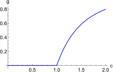
Figure 1: (Color online) The probability $g$ that a random node in an ER network resides on the giant component, as a function of the mean degree, $c$. For $c<1$ there is no giant component and thus $g=0$. At $c=1$ there is a percolation transition, above which $g$ increases monotonically towards the dense network limit of $g=1$.

which is known as the Molloy-Reed criterion Molloy1995 ; Molloy1998 . In essence, this criterion states that a giant component exists if the mean excess degree of the neighbours of a random node exceeds one. In Fig. 1 we present the parameter $g$, which is the probability that a random node resides on the giant component, for an ER network, as a function of the mean degree, $c$. For $c<1$ there is no giant component and thus $g=0$. The percolation transition takes place at $c=1$, above which $g$ gradually increases towards the dense network limit of $g=1$.

III The Degree Distribution on the Giant Component

The probability, $g$, that a randomly selected node belongs to the giant component can be expressed in the form

$$g=\sum_{k=0}^{\infty}g_{k}P(k),$$ (9)

where $g_{k}$ is the conditional probability that a random node belongs to the giant component, given that its degree is $k$. Comparing this expression to Eq. (7) we find that

$$g_{k}=1-(1-\tilde{g})^{k}.$$ (10)

To make the conditioning explicit, we introduce an indicator variable $\Lambda\in\{0,1\}$, with $\Lambda=1$ indicating that an event happens on the giant component, whereas $\Lambda=0$ indicates that it happens on one of the finite components of the network. The probability that a random node resides on the giant component is given by $P(\Lambda=1)=g$, while the probability that it resides on one of the finite components is $P(\Lambda=0)=1-g$. The probability that a random node of a given degree $k$ resides on the giant component is given by

$$P(\Lambda=1|K=k)=g_{k}=1-(1-\tilde{g})^{k},$$ (11)

while the probability that it resided on one of the finite components is

$$P(\Lambda=0|K=k)=1-g_{k}=(1-\tilde{g})^{k}.$$ (12)

Using Bayes’ theorem

$$P(K=k|\Lambda=\lambda)=\frac{P(\Lambda=\lambda|K=k)}{P(\Lambda=\lambda)}P(K=k),$$ (13)

we invert these relations so as to obtain the degree distributions conditioned on a node to belong to the giant and the finite components, respectively. For brevity, in the rest of the paper we use a more compact notation, in which $P(K=k)$, $P(\Lambda=\lambda)$ and $P(K=k|\Lambda=\lambda)$ are replaced by $P(k)$, $P(\lambda)$ and $P(k|\lambda)$, respectively, except for a few places in which the more detailed notation is needed for clarity. The conditional degree distribution of nodes which reside on the giant component is given by

$$P(k|1)=\frac{1-(1-\tilde{g})^{k}}{g}P(k),$$ (14)

while the conditional degree distribution for nodes which reside on the finite tree components is

$$P(k|0)=\frac{(1-\tilde{g})^{k}}{1-g}P(k).$$ (15)

This result can be expressed in the form

$$P(k|0)=\frac{1}{1-g}e^{-ak}P(k),$$ (16)

where $a=-\ln(1-\tilde{g})$. This highlights the fact that the degree distribution of the finite components is an exponentially attenuated variant of the original degree distribution. The result for the finite components, Eq. (15), was first derived by Molloy and Reed Molloy1995 ; Molloy1998 (although in a less transparent form), while the result for the giant component, Eq. (14), was reported by Engel et al. Engel2004 for the special case of ER networks (for which $\tilde{g}=g$).

The mean degree conditioned on the giant component is

$$c_{1}=\mathbb{E}[K|1]=\sum_{k=1}^{\infty}kP(k|1).$$ (17)

Using Eq. (14) and performing the summation, we obtain

$$c_{1}=\frac{c}{g}\left[1-(1-\tilde{g})^{2}\right]=\frac{(2-\tilde{g})\tilde{g}}{g}c.$$ (18)

The mean degree conditioned on the finite components is given by

$$c_{0}=\mathbb{E}[K|0]=\sum_{k=0}^{\infty}kP(k|0).$$ (19)

From Eq. (15), we obtain

$$c_{0}=\frac{(1-\tilde{g})^{2}}{1-g}c.$$ (20)

Using Eq. (15) and the generating function $G_{1}(x)$, it can be shown that $(1-\tilde{g})^{2}/(1-g)<1$ for $0<\tilde{g}<1$, which implies that $c_{0}<c$ and $c_{1}>c$. For ER networks these results specialize to $c_{1}=(2-g)c$ and $c_{0}=(1-g)c$, respectively. Actually, the value of $c_{0}$ corresponds to the mean degree below the percolation threshold as it must correspond to a sub-percolating configuration model.

In the literature, the finite component result of Eq. (15) is referred to as a discrete duality relation Molloy1998 ; Bollobas2007 ; Janson2010 . Indeed for ER networks $P(k|0)$ is in itself a Poisson distribution of the form

$$P(k|0)=\frac{e^{-c_{0}}c_{0}^{k}}{k!},$$ (21)

where $c_{0}=c(1-g)$ is the mean degree of the nodes which reside on the finite components. The degree distribution, restricted to nodes on the finite components of an ER network is thus of the same type as the degree distribution of the entire network, albeit with a renormalized parameter for the mean degree, $c_{0}$. Note that $c_{0}<1$ for any $c>1$, reflecting the fact that the finite components are equivalent to a sub-percolating ER network.

An analogous parametric renormalization relating the degree distribution of the whole network to a degree distribution conditioned on the finite components is found for any degree distribution which has a component which scales exponentially in $k$. Such degree distributions can be expressed in the form

$$P(k)=\phi(k)e^{-\alpha k},$$ (22)

where $\alpha>0$, and the function $\phi(k)\geq 0$ is chosen such that $P(k)$ is properly normalized. Clearly, the simplest example of such degree distribution is the exponential distribution, for which $\phi(k)=1-e^{-\alpha}$ is merely a normalization constant. For networks with an exponential component in the degree distribution as described in Eq. (22), the degree distribution conditioned on the finite components takes the form

$$P(k|0)=\frac{1}{1-g}\phi(k)e^{-\alpha_{0}k}$$ (23)

with $\alpha_{0}=\alpha-\ln(1-\tilde{g})$. This simple parametric renormalization with respect to Eq. (22) is in close analogy to the results obtained earlier for ER networks. The degree distribution conditioned on the giant component can be compactly expressed as

$$P(k|1)=\frac{e^{-\alpha k}-e^{-\alpha_{0}k}}{g}\phi(k).$$ (24)

In order to obtain the conditional degree distributions for a given network, one needs to evaluate the parameters $g$ and $\tilde{g}$. The latter is obtained from the solution of Eq. (6), while the former is obtained by inserting the solution for $\tilde{g}$ into (7).

IV Degree-Degree Correlations on the Giant Component

Having computed degree distributions conditioned on the giant and finite components of configuration model networks, we now turn to investigating the micro-structure of these giant and finite components further by looking at various joint degree distributions and degree-degree correlation. We shall find that — on the giant component — there are degree-degree correlations of any order. This could have been anticipated, as degree-degree correlations of arbitrarily high order are clearly required in order to exclude the possibility that a randomly selected node belongs to a tree of any finite size. In what follows we go some way to quantify these correlations. The key step is to use Eq. (6) to express the powers $(1-\tilde{g})^{k}$ appearing in Eq. (7), resulting in

$$g=\sum_{k;\{k_{\mu}\}}\left[1-\prod_{\mu=1}^{k}(1-\tilde{g})^{k_{\mu}-1}\right]P(k)\prod_{\mu=1}^{k}\frac{k_{\mu}}{c}P(k_{\mu}).$$ (25)

Here we use the notation $k;\{k_{\mu}\}$ to denote a configuration consisting of a central node of degree $k$, surrounded by a first coordination shell of nodes with degrees $k_{\mu},\mu=1,\dots,k$. The probabilistic interpretation of this identity is that the probability that a random node of degree $k$, whose neighbors are of degrees $k_{1},\dots,k_{k}$ resides on the giant component is

$$P(1|k;\{k_{\mu}\})=\left[1-\prod_{\mu=1}^{k}(1-\tilde{g})^{k_{\mu}-1}\right],$$ (26)

while the probability that it resides on one of the finite components is

$$P(0|k;\{k_{\mu}\})=\prod_{\mu=1}^{k}(1-\tilde{g})^{k_{\mu}-1}.$$ (27)

Using Bayes’ Theorem, one can invert these relations to obtain

$$P(k;\{k_{\mu}\}|1)=\frac{1}{g}\left[1-\prod_{\mu=1}^{k}(1-\tilde{g})^{k_{\mu}-1}\right]P(k)\prod_{\mu=1}^{k}\frac{k_{\mu}}{c}P(k_{\mu}),$$ (28)

and

$$P(k;\{k_{\mu}\}|0)=\frac{1}{1-g}\left[\prod_{\mu=1}^{k}(1-\tilde{g})^{k_{\mu}-1}\right]P(k)\prod_{\mu=1}^{k}\frac{k_{\mu}}{c}P(k_{\mu}),$$ (29)

as the probabilities for nodes to have a degree $k$ and first neighbour shell configuration $k_{1},\dots,k_{k}$, conditioned on this happening on the giant component, and on one of the finite components, respectively. Note that Eq. (14) correctly predicts that the probability of a node of degree $k=0$ to belong to the giant component is zero. Moreover, Eq. (28) also correctly predicts that the probability of a node of degree $k$ to connect to $k$ nodes of degree $1$, thereby forming an isolated $(k+1)$-star, is zero on the giant component.

Marginalizing $P(k;\{k_{\mu}\}|1)$, namely summing Eq. (28) over all the values of $k_{2},\dots,k_{k}$, and replacing $k_{1}\rightarrow k^{\prime}$, gives the probability of a random node of degree $k$ to be connected to a node of degree $k^{\prime}$, conditioned on them being on the giant component

$$P(k;k^{\prime}|1)=\frac{1}{g}\left[1-(1-\tilde{g})^{k-1}(1-\tilde{g})^{k^{\prime}-1}\right]P(k)\frac{k^{\prime}}{c}P(k^{\prime}),\quad k\geq 1.$$ (30)

Similarly, from Eq. (29) we obtain the probability of a random node of degree $k$ to be connected to a node of degree $k^{\prime}$, under the condition that they do not reside on the giant component

$$P(k;k^{\prime}|0)=\frac{1}{1-g}(1-\tilde{g})^{k-1}(1-\tilde{g})^{k^{\prime}-1}P(k)\frac{k^{\prime}}{c}P(k^{\prime}),\quad k\geq 1.$$ (31)

Here we have exploited the fact that the $k_{2},\dots,k_{k}$ averages over the distributions of neighbouring degrees factor, each of them giving

$$\sum_{k_{\mu}}(1-\tilde{g})^{k_{\mu}-1}\frac{k_{\mu}}{c}P(k_{\mu})=1-\tilde{g},$$ (32)

by using Eq. (6). Marginalizing Eqs. (30) and (31) by summing over $k^{\prime}$, we recover $P(k|1)$ and $P(k|0)$ as given by Eqs. (14) and (15). On the other hand, marginalizing Eq. (30) by summing over $k\geq 1$, gives the probability, starting from a randomly chosen node on the giant component, to reach a node of degree $k^{\prime}$, namely

$$\widetilde{P}(k^{\prime}|1)\equiv\sum_{k\geq 1}P(k;k^{\prime}|1).$$ (33)

Carrying out the summation we obtain

$$\widetilde{P}(k^{\prime}|1)=\frac{1}{g}\left[1-p_{0}-\frac{1-g-p_{0}}{1-\tilde{g}}(1-\tilde{g})^{k^{\prime}-1}\right]\frac{k^{\prime}}{c}P(k^{\prime}),$$ (34)

where $p_{0}=P(K=0)$, namely the probability of an isolated node in the original network. It is easy to see that this is a normalized distribution. It is also important to stress the asymmetric role of the two degrees $k$ and $k^{\prime}$ appearing in Eqs. (30) and (31).

Consider a random edge in a configuration model network. The joint degree distribution, $\widehat{P}(k,k^{\prime})$, of the nodes which reside on both sides of such edge is given by

$$\widehat{P}(k,k^{\prime})=\frac{k}{c}P(k)\frac{k^{\prime}}{c}P(k^{\prime}).$$ (35)

The non-giant components of a configuration model network constitute a sub-network which is itself a configuration model network, and is in the sub-percolation regime. The degree distribution, $P(k|0)$, of this sub-network is given by Eq. (15). Thus, the joint degree distribution of pairs of connected nodes which reside on the non-giant components is given by

$$\widehat{P}(k,k^{\prime}|0)=\frac{(1-\tilde{g})^{k-1}(1-\tilde{g})^{k^{\prime}-1}}{(1-\tilde{g})^{2}}\frac{k}{c}P(k)\frac{k^{\prime}}{c}P(k^{\prime}).$$ (36)

The fraction of edges in the network which reside on the giant component is denoted by $g_{E}$. It is given by

$$g_{E}=1-(1-\tilde{g})^{2},$$ (37)

while the fraction of edges which reside on the non-giant components is $1-g_{E}=(1-\tilde{g})^{2}$. Therefore, the joint degree distribution can be expressed in the form

$$\widehat{P}(k,k^{\prime})=\left[1-(1-\tilde{g})^{2}\right]\widehat{P}(k,k^{\prime}|1)+(1-\tilde{g})^{2}\widehat{P}(k,k^{\prime}|0).$$ (38)

Using Eqs. (36) and (38) we find that

$$\widehat{P}(k,k^{\prime}|1)=\frac{1-(1-\tilde{g})^{k+k^{\prime}-2}}{1-(1-\tilde{g})^{2}}\frac{k}{c}P(k)\frac{k^{\prime}}{c}P(k^{\prime}).$$ (39)

V Assortativity on the Giant Component

From the joint probability $\widehat{P}(k,k^{\prime}|1)$ that a randomly chosen edge on the giant component connects two vertices of degrees $k$ and $k^{\prime}$, one obtains the corresponding probability for a random edge to connect nodes of excess-degrees $k$ and $k^{\prime}$, by a simple shift of arguments as

$$\widehat{P}_{e}(k,k^{\prime}|1)=\widehat{P}(k+1,k^{\prime}+1|1).$$ (40)

The conditional joint probability of excess degrees, $\widehat{P}_{e}(k,k^{\prime}|1)$, is given by

$$\widehat{P}_{e}(k,k^{\prime}|1)=\left[\frac{1-(1-\tilde{g})^{k+k^{\prime}-2}}{1-(1-\tilde{g})^{2}}\right]\frac{k+1}{c}P(k+1)\frac{k^{\prime}+1}{c}P(k^{\prime}+1).$$ (41)

Summing over $k$, we obtain the marginal distribution

$$\widehat{P}_{e}(k|1)=\left[\frac{1-(1-\tilde{g})^{k-1}}{1-(1-\tilde{g})^{2}}\right]\frac{k+1}{c}P(k+1).$$ (42)

In terms of these definitions, the assortativity coefficient on the giant component is given by Newman2002b

$$r=\frac{1}{\hat{\sigma}^{2}}\sum_{k,k^{\prime}\geq 0}kk^{\prime}\left[\widehat{P}_{e}(k,k^{\prime}|1)-\widehat{P}_{e}(k|1)\widehat{P}_{e}(k^{\prime}|1)\right],$$ (43)

where

$$\hat{\sigma}^{2}=\sum_{k\geq 0}k^{2}\widehat{P}_{e}(k|1)-\left[\sum_{k\geq 0}k\widehat{P}_{e}(k|1)\right]^{2}$$ (44)

is the variance of $\widehat{P}_{e}(k|1)$. The assortativity coefficient is actually the Pearson correlation coefficient of degrees between pairs of linked nodes Newman2002b .

While the assortativity coefficient can be evaluated directly from Eq. (43), it turns out that there is a more effective approach for its calculation, using generating functions. To this end, we introduce the bivariate generating function, $B(u,v)$, of $\widehat{P}_{e}(k,k^{\prime}|1)$, which is given by

$$B(u,v)=\sum_{k,k^{\prime}\geq 0}\widehat{P}_{e}(k,k^{\prime}|1)u^{k}v^{k^{\prime}}.$$ (45)

This function is symmetric in $u$ and $v$, reflecting the symmetric form of $\widehat{P}_{e}(k,k^{\prime}|1)$ in terms of $k$ and $k^{\prime}$. We also introduce the generating function, $S(u)$, of the marginal distribution $\widehat{P}_{e}(k|1)$, which takes the form

$$S(u)=\sum_{k\geq 0}\widehat{P}(k|1)u^{k}.$$ (46)

Note that it can be expressed in terms of the bivariate generating function, as $S(u)=B(u,1)$. Inserting the expression for $\widehat{P}_{e}(k,k^{\prime}|1)$ from Eq. (41) into Eq. (45), we find that the bivariate generating function $B(u,v)$ can be expressed in terms of the generating function $G_{1}(x)$ of the degree distribution $P(k)$. It takes the form

$$B(u,v)=\frac{G_{1}(u)G_{1}(v)-G_{1}[(1-\tilde{g})u]G_{1}[(1-\tilde{g})v]}{1-(1-\tilde{g})^{2}}.$$ (47)

Plugging in $v=1$ we obtain

$$S(u)=\frac{G_{1}(u)-(1-\tilde{g})G_{1}[(1-\tilde{g})u]}{1-(1-\tilde{g})^{2}}.$$ (48)

Expressing the terms on the right hand side of Eq. (43) in terms of derivatives of the generating functions $B(u,v)$ and $S(u)$, we express the assortativity coefficient in the form

$$r=\frac{\partial_{u}\partial_{v}B(u,v)-[\partial_{u}S(u)]^{2}}{(u\partial_{u})^{2}S(u)-[\partial_{u}S(u)]^{2}}\,\Bigg{|}_{u=v=1}.$$ (49)

In the next section we use this formulation to obtain exact analytical results for the assortativity coefficients on the giant components of different configuration model networks. The assortativity coefficient is expected to be negative, which implies that the giant component of a configuration model network is disassortative. This is due to the fact that high-degree nodes are over-represented in the giant component. Thus, in order that the giant component will be a single connected component, low degree nodes must have a greater than normal probability to connect to high degree nodes. In particular, a node of degree $k=1$ on the giant component must be connected to a node of degree $k^{\prime}\geq 2$, while a node of degree $k=2$ can have at most one neighbor of degree $k^{\prime}=1$. The disassortativity of the giant component is most pronounced just above the percolation threshold, where most nodes are of low degrees.

VI Analysis of specific network models

In this section we discuss in detail some specific network models and the properties of their giant components.

VI.1 Erdős-Rényi networks

Consider an ER network of $N$ nodes and mean degree $c>1$. In this case the degree distribution follows a Poisson distribution, given by Eq. (3). The generating functions $G_{0}$ and $G_{1}$ of this distribution coincide and satisfy

$$G_{0}(x)=G_{1}(x)=e^{-c(1-x)}.$$ (50)

As a result, in this case $\tilde{g}=g$. Using Eq. (7) one obtains a closed form expression for $g$, which is given by

$$g=1+\frac{W(-ce^{-c})}{c},$$ (51)

where $W(x)$ is the Lambert W function Olver2010 . In this case a giant component exists for $c>1$ (Fig. 1). The degree distribution on the giant component is obtained from Eq. (14), where $g$ and $\tilde{g}$ are given by Eq. (51). It is given by

$$P(k|1)=\frac{1}{g}\left[\frac{e^{-c}c^{k}}{k!}-(1-g)\frac{e^{-c(1-g)}[c(1-g)]^{k}}{k!}\right],$$ (52)

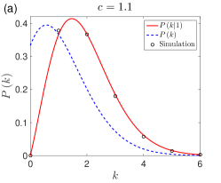
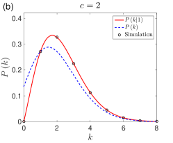
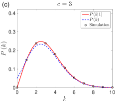
Figure 2: (Color online) Analytical results for the degree distribution, $P(k|1)$, of the giant component of an ER network (solid lines), obtained from Eq. (52), for $c=1.1$ (a), $c=2$ (b) and $c=3$ (c). The analytical results are in excellent agreement with the results of computer simulations (circles), for a network of $N=1000$ nodes. For comparison, the degree distribution, $P(k)$, of the whole network, obtained from Eq. (3) is also shown (dashed lines).

which takes the form of the difference between two Poisson distributions. In Fig. 2 we present analytical results for the degree distribution, $P(k|1)$, of the giant components of ER networks with mean degrees $c=1.1$, $2$ and $3$ (solid lines), obtained from Eq. (52). The analytical results are found to be in excellent agreement with the results of computer simulations (circles), for a network of size $N=1000$. For comparison we also show the degree distribution on the entire network (dashed lines), obtained from Eq. (3).

The mean degree of the giant component of an ER network, obtained from Eq. (17), is given by

$$\mathbb{E}[K|1]=(2-g)c,$$ (53)

while the mean degree of the finite components, obtained from Eq. (20) is

$$\mathbb{E}[K|0]=(1-g)c.$$ (54)

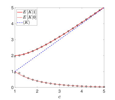
Figure 3: (Color online) Analytical results for the mean degree of the giant component, $\mathbb{E}[K|1]$, of an ER network (solid line), as a function of $c$, for $c\geq 1$, obtained from Eq. (53). The analytical results are found to be in excellent agreement with the results of computer simulations (circles), for a network of $N=1000$ nodes. For comparison, the mean degree, $\langle K\rangle=c$, of the whole network is also shown (dashed line). The mean degree of the giant component starts from $\mathbb{E}[K|1]=2$ at $c=1$ and gradually approaches the result for the whole network as $c$ is increased. In contrast, the mean degree, $\mathbb{E}[K|0]$, of the finite components (dotted line) starts from $\mathbb{E}[K|0]=1$ at $c=1$ and gradually decreases to zero as $c$ is increased.

In Fig. 3 we present analytical results for the mean degree, $\mathbb{E}[K|1]$, of the giant component (solid line) and the mean degree, $\mathbb{E}[K|0]$, of the finite components (dotted line), of an ER network as a function of $c$. The mean degree of the whole network, $\langle K\rangle=c$, is also shown (dashed line). It is observed that at the percolation threshold ($c=1$), $\mathbb{E}[K|1]=2$, while $\langle K\rangle=1$. As $c$ is increased, the mean degree of the giant component converges asymptotically towards to overall mean degree of the network, while the mean degree of the finite components decays to zero.

The assortativity coefficient for the giant component of an ER network is given by

$$r=-\frac{c(1-g)^{2}}{(2-g)^{3}-(1-g)(2-g)-c(1-g)^{2}}.$$ (55)

In the limit of large $c$, the index $r$ decreases according to $r\simeq-ce^{-2c}$. For values of $c$ just above the percolation threshold, we find that

$$r\simeq-\frac{1}{5}+\frac{12}{25}(c-1)^{2}+{\mathcal{O}}\left[(c-1)^{3}\right].$$ (56)

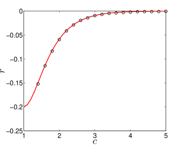
Figure 4: (Color online) The assortativity coefficient $r$ of the giant component of an ER network, as a function of $c$. The analytical results (solid line), obtained from Eq. (55), are found to be in excellent agreement with the results of computer simulations (circles), performed for networks of size $N=5000$. The negative values of $r$ imply that the giant component is disassortative, namely high degree nodes preferentially connect to low degree nodes and vice versa. As $c$ is increased, the giant component encompasses an increasing fraction of the entire network, and $r$ decays to zero.

The negative value of $r$ implies that the giant component is disassortative, meaning that high degree nodes on the giant component tend to connect to low degree nodes and vice versa. As $c$ is increased, the absolute value of $r$ gradually decreases. In Fig. 4 we present the assortativity coefficient, $r$, of the giant component of an ER network, as a function of $c$. Just above the percolation transition, the assortativity coefficient is large and negative. Its absolute value gradually decreases and eventually vanishes as $c$ is increased, reflecting the fact that the giant component coincides with the entire network, and all the correlations are lost.

VI.2 Configuration model networks with an exponential degree distribution

Consider a configuration model network with an exponential degree distribution of the form

$$P(k)=Ae^{-\alpha k},$$ (57)

where $k\geq k_{\rm min}$. Here we focus on the case of $k_{\rm min}=1$, for which the normalization factor is $A=e^{\alpha}-1$. The mean degree is given by

$$c=\langle K\rangle=\frac{1}{1-e^{-\alpha}}.$$ (58)

For the analysis presented below, it is convenient to parametrize the degree distribution in terms of the mean degree, $c$. Plugging in $\alpha=\ln c-\ln(c-1)$ we obtain

$$P(k)=\frac{1}{c}\left(\frac{c-1}{c}\right)^{k-1},$$ (59)

with $k\geq 1$. The degree generating function $G_{0}(x)$ is given by

$$G_{0}(x)=\frac{x}{c-x(c-1)}.$$ (60)

It exhibits two trivial fixed points, namely $G_{0}(0)=0$ and $G_{0}(1)=1$. The cavity generating function $G_{1}(x)$ is

$$G_{1}(x)=\frac{1}{\left[c-x(c-1)\right]^{2}}.$$ (61)

This generating function has a trivial fixed point given by $G_{1}(1)=1$. The size of the giant component is obtained using a two step process. In the first step we find the non-trivial fixed point of $G_{1}(x)$, by solving Eq. (6) for $\tilde{g}$. We find that

$$\tilde{g}=\frac{c-3}{2(c-1)}+\frac{1}{2}\sqrt{\frac{c+3}{c-1}}.$$ (62)

In the second step we obtain the fraction of nodes which reside on the giant component, which is given by Eq. (7), namely

$$g=\frac{3c}{2(c-1)}-\frac{c(c+3)^{1/2}}{2(c-1)^{3/2}}.$$ (63)

The percolation transition occurs at $c=3/2$, such that a giant component exists for $c>3/2$. The degree distribution on the giant component, obtained from Eq. (14), takes the form

$$P(k|1)=\left[\frac{1-(1-\tilde{g})^{k}}{(c-1)g}\right]\left(\frac{c-1}{c}\right)^{k},$$ (64)

where $\tilde{g}$ is given by Eq. (62) and $g$ is given by Eq. (63). The mean degree on the giant component is given by Eq. (18). The assortativity coefficient of a configuration model with an exponential degree distribution takes the form

$$r=-\frac{2(c-1)(1-\tilde{g})^{2}[1-(1-\tilde{g})^{3/2}]^{2}}{[1-(1-\tilde{g})^{2}]\{1-(1-\tilde{g})^{7/2}+3(c-1)[1-(1-\tilde{g})^{5}]\}-2(c-1)[1-(1-\tilde{g})^{7/2}]^{2}}.$$ (65)

In the limit of large $c$, the assortativity coefficient decreases to zero according to

$$r\simeq-2c^{-4}+2c^{-5}+{\mathcal{O}}(c^{-6}).$$ (66)

Just above the percolation threshold, which is located at $c=3/2$, the assortativity coefficient can be approximated by

$$r\simeq-\frac{3}{13}+\frac{2240}{1521}\left(c-\frac{3}{2}\right)^{2}-\frac{35840}{13689}\left(c-\frac{3}{2}\right)^{3}+{\mathcal{O}}\left(c-\frac{3}{2}\right)^{4}.$$ (67)

VI.3 Configuration model networks with a ternary degree distribution

The properties of the giant components of random networks are very sensitive to the abundance of nodes of low degrees, particularly nodes of degree $k=1$ (leaf nodes) and $k=2$. Nodes of degree $k=0$ (isolated nodes) are excluded from the giant component and their weight in the overall degree distribution has no effect on the properties of the giant component. Therefore, it is useful to consider a simple configuration model in which all nodes are restricted to a small number of low degrees. Here we consider a configuration model network with a ternary degree distribution of the form Newman2010

$$P(k)=p_{1}\delta_{k,1}+p_{2}\delta_{k,2}+p_{3}\delta_{k,3},$$ (68)

where $\delta_{k,n}$ is the Kronecker delta, and $p_{1}+p_{2}+p_{3}=1$. The mean degree of such network is given by

$$\langle K\rangle=p_{1}+2p_{2}+3p_{3}.$$ (69)

The generating functions are

$$G_{0}(x)=p_{1}x+p_{2}x^{2}+p_{3}x^{3},$$ (70)

and

$$G_{1}(x)=\frac{p_{1}+2p_{2}x+3p_{3}x^{2}}{p_{1}+2p_{2}+3p_{3}}.$$ (71)

Solving Eq. (6) for $\tilde{g}$, with $G_{1}(x)$ given by Eq. (71), we find that

$$\tilde{g}=\begin{dcases}0&\ \ \ \ p_{3}\leq\frac{p_{1}}{3}\\ 1-\frac{p_{1}}{3p_{3}}&\ \ \ \ p_{3}>\frac{p_{1}}{3}.\end{dcases}$$ (72)

And using Eq. (7) for $g$, where $G_{0}(x)$ is given by Eq. (70), we find that

$$g=\begin{dcases}0&\ \ \ \ p_{3}\leq\frac{p_{1}}{3}\\ 1-\frac{p_{1}^{2}}{3p_{3}}-\frac{p_{1}^{2}p_{2}}{9p_{3}^{2}}-\frac{p_{1}^{3}}{27p_{3}^{2}}&\ \ \ \ p_{3}>\frac{p_{1}}{3}.\end{dcases}$$ (73)

Thus, the percolation threshold is located at $p_{3}=p_{1}/3$. This can be understood intuitively by recalling that the finite components exhibit tree structures. In a tree that includes a single node of degree $k=3$, with three chains of arbitrary lengths attached to it, there must be three leaf nodes of degree $k=1$. In more complex tree structures, let alone in the giant component, there must be more than one node of degree $3$ for every three nodes of degree $1$. This is not likely to occur in case that $p_{3}<p_{1}/3$. Using the normalization condition, we find that for any given value of $p_{2}$, a giant component exists for $p_{3}>(1-p_{2})/4$.

The degree distribution on the giant component is given by

$$P(k|1)=\frac{1-\left(\frac{p_{1}}{3p_{3}}\right)^{k}}{1-\left(\frac{p_{1}^{2}}{3p_{3}}\right)-\left(\frac{p_{1}^{2}p_{2}}{9p_{3}^{2}}\right)-\left(\frac{p_{3}}{27p_{3}^{2}}\right)}P(k),$$ (74)

where $k=1,2,3$ and $P(k)$ is given by Eq. (68). The degree distribution on the finite components is given by

$$P(k|0)=\frac{\left(\frac{p_{1}}{3p_{3}}\right)^{k}}{\left(\frac{p_{1}^{2}}{3p_{3}}\right)+\left(\frac{p_{1}^{2}p_{2}}{9p_{3}^{2}}\right)+\left(\frac{p_{3}}{27p_{3}^{2}}\right)}P(k).$$ (75)

Thus, the mean degree on the giant component is given by

$$\mathbb{E}[k|1]=\frac{1-\left(\frac{p_{1}}{3p_{3}}\right)^{k}}{1-\left(\frac{p_{1}^{2}}{3p_{3}}\right)-\left(\frac{p_{1}^{2}p_{2}}{9p_{3}^{2}}\right)-\left(\frac{p_{3}}{27p_{3}^{2}}\right)}\langle K\rangle,$$ (76)

while the mean degree on the finite components is given by

$$\mathbb{E}[k|0]=\frac{\left(\frac{p_{1}}{3p_{3}}\right)^{k}}{\left(\frac{p_{1}^{2}}{3p_{3}}\right)+\left(\frac{p_{1}^{2}p_{2}}{9p_{3}^{2}}\right)+\left(\frac{p_{3}}{27p_{3}^{2}}\right)}\langle K\rangle.$$ (77)

The assortativity coefficient of the ternary network is given by

$$r=-\frac{18p_{1}^{2}p_{3}^{2}}{27p_{2}p_{3}^{3}+9p_{1}^{2}p_{3}(p_{2}+2p_{3})+27p_{1}p_{3}^{2}(p_{2}+2p_{3})+p_{1}^{3}(p_{2}+6p_{3})}.$$ (78)

As $p_{3}$ is increased, while keeping $p_{2}$ fixed, the network becomes denser and the fraction of nodes, $g$, which reside on the giant component increases, reaching $g=1$ at $p_{3}=1-p_{2}$ (namely, at the point in which the number of leaf nodes vanishes). Above this point the giant component encompasses the entire network and the assortativity coefficient $r$ vanishes. In the opposite case, in which $p_{3}$ is decreased the network becomes more sparse. The percolation transition takes place at $p_{3,c}=(1-p_{2})/4$. In the limit of sparse networks just above the percolation threshold the assortativity coefficient can be approximated by

$$r\simeq-3\frac{1-p_{2}}{9+7p_{2}}-64p_{2}\frac{p_{3}-p_{3,c}}{(9+7p_{2})^{2}}+{\cal{O}}\left[(p_{3}-p_{3,c})^{2}\right].$$ (79)

In the limit of $p_{3}\rightarrow 1$ (and $p_{1},p_{2}\rightarrow 0$), the ternary network becomes a random regular graph (RRG) with a degenerate degree distribution of the form $P(k)=\delta_{k,3}$, while in the limit of $p_{2}\rightarrow 1$ (and $p_{1},p_{3}\rightarrow 0$) it becomes an RRG with $P(k)=\delta_{k,2}$. In general, random regular graphs exhibit degree distributions of the form $P(k)=\delta_{k,c}$, where $c\geq 2$ is an integer. In RRGs with $c\geq 3$ the giant component encompasses the entire network, namely $g=\tilde{g}=1$ Bonneau2017 . Thus, the degree distribution of the giant component is simply $P(k)=\delta_{k,c}$.

The case of an RRG with $c=2$, which corresponds to the limit of $p_{2}\rightarrow 1$ and $p_{1},p_{3}\rightarrow 0$, is special. An RRG with $c=2$ consists of a collection of closed cycles. The local structure of all the cycles is identical, and follows the overall degree distribution of the network, $P(k)=\delta_{k,2}$. Thus, unlike the case of other configuration model networks there is no further information to be revealed about the degree distribution of the giant component. The generating function method used in this paper does not permit the calculation of the percolating fraction, $g$, in the case of RRGs with $c=2$, as the value of $g$ turns out to be indeterminate in this case. However, an interesting analogy between the cycles of RRGs with $c=2$ and the cycles which appear in they theory of random permutations, enables one to conclude that the average size of the longest cycle is extensive in $N$. In random permutations of $N$ objects, the average length of the longest cycle turns out to be $gN$ where $g\simeq 0.62455$ is the Golomb-Dickman constant Shepp1966 . However, in numerical simulations of RRGs with $c=2$ we found that the average length of the longest cycle is given by $gN$, where $g\simeq 0.755$. This difference can be understood from the fact that the two systems differ in some details. For example, unlike the case of random permutations, in RRGs with $c=2$ fixed points (namely isolated nodes) and cycles of length $2$ (namely dimers) are not allowed, and the minimal cycle length is $3$.

VI.4 Configuration model networks with a Zipf degree distribution

Consider a configuration model network with a Zipf degree distribution of the form

$$P(k)=\frac{e^{\alpha k_{\rm min}}}{\Phi(e^{-\alpha},1,k_{\rm min})}\frac{e^{-\alpha k}}{k},$$ (80)

where $\Phi(z,s,k)$ is the Lerch transcendent function Olver2010 . This distribution exhibits a power-law component of the form $k^{-\gamma}$, with $\gamma=1$, with a cutoff in the form of an exponential tail controlled by the parameter $\alpha$, which sets the range of the tail. The mean degree is given by

$$\langle K\rangle=\frac{\Phi(e^{-\alpha},0,k_{\rm min})}{\Phi(e^{-\alpha},1,k_{\rm min})}.$$ (81)

The generating functions take the form

$$G_{0}(x)=x^{k_{\rm min}}\Phi(xe^{-\alpha},1,k_{\rm min}),$$ (82)

and

$$G_{1}(x)=\frac{x^{k_{\rm min}-1}\Phi(xe^{-\alpha},0,k_{\rm min})}{\Phi(e^{-\alpha},0,k_{\rm min})}.$$ (83)

Note that $G_{0}(0)=0$ and $G_{0}(1)=G_{1}(1)=1$.

From this point and on, we focus on the case $k_{min}=1$, where many of the quantities mentioned above become significantly simpler. In particular, the mean degree becomes

$$\langle K\rangle=\frac{-1}{(e^{\alpha}-1)\ln(1-e^{-\alpha})},$$ (84)

and the two degree generating functions become

$$G_{0}(x)=\frac{\ln\left(1-e^{-\alpha}x\right)}{\ln\left(1-e^{-\alpha}\right)},$$ (85)

and

$$G_{1}(x)=\frac{1-e^{-\alpha}}{1-e^{-\alpha}x}.$$ (86)

Inserting the expression of $G_{1}(x)$ given by Eq. (86) into Eq. (6) we find that there is a non-trivial solution of the form

$$\tilde{g}=2-e^{\alpha}.$$ (87)

Using Eq. (7) we find that

$$g=1+\frac{\alpha}{\ln(1-e^{-\alpha})}.$$ (88)

The percolation transition takes place at $\alpha=\ln 2$, below which there is a giant component. The degree distribution $P(k|1)$ on the giant component is given by Eq. (14), where $\tilde{g}$ is given by Eq. (87) and $g$ is given by Eq. (88). The mean degree on the giant component is given by

$$\mathbb{E}[K|1]=\frac{e^{\alpha}-2}{(1-e^{-\alpha})\left[\alpha+\ln(1-e^{-\alpha})\right]}.$$ (89)

The assortativity index is given by

$$r=-\frac{(1-e^{-\alpha})^{2}}{e^{2\alpha}-3e^{\alpha}+3}.$$ (90)

For small values of $\alpha$ we obtain

$$r\simeq-\alpha^{2}-\frac{\alpha^{4}}{12}+{\mathcal{O}}\left(\alpha^{6}\right).$$ (91)

For values of $\alpha$ just above the percolation threshold, we obtain

$$r\simeq-\frac{1}{4}+\frac{5}{4}\left(\alpha-\ln 2\right)^{2}+{\mathcal{O}}\left[\left(\alpha-\ln 2\right)^{3}\right].$$ (92)

VI.5 Configuration model networks with a power-law degree distribution

Consider a configuration model network with a power-law degree distribution of the form

$$P(k)=\frac{A}{k^{\gamma}}$$ (93)

for $k_{\rm min}\leq k\leq k_{\rm max}$, where the normalization coefficient is

$$A=\frac{1}{\zeta(\gamma,k_{\rm min})-\zeta(\gamma,k_{\rm max}+1)}$$ (94)

and $\zeta(s,a)$ is the Hurwitz zeta function Olver2010 . The mean degree is given by

$$\langle K\rangle=\frac{\zeta(\gamma-1,k_{\rm min})-\zeta(\gamma-1,k_{\rm max}+1)}{\zeta(\gamma,k_{\rm min})-\zeta(\gamma,k_{\rm max}+1)},$$ (95)

while the second moment of the degree distribution is

$$\langle K^{2}\rangle=\frac{\zeta(\gamma-2,k_{\rm min})-\zeta(\gamma-2,k_{\rm max}+1)}{\zeta(\gamma,k_{\rm min})-\zeta(\gamma,k_{\rm max}+1)}.$$ (96)

For $\gamma\leq 2$ the mean degree diverges when $k_{\rm max}\rightarrow\infty$. For $2<\gamma\leq 3$ the mean degree is bounded while the second moment, $\langle K^{2}\rangle$, diverges. For $\gamma>3$ both moments are bounded. For $\gamma>2$ and $k_{\rm min}\geq 2$ (where nodes of degrees $0$ and $1$ do not exist), $\langle K^{2}\rangle>2\langle K\rangle$ namely the Molloy and Reed criterion is satisfied and the network exhibits a giant component Molloy1995 ; Molloy1998 . Moreover, under these conditions the giant component encompasses the entire network Bonneau2017 .

The case of $k_{\rm min}=1$ is particularly interesting. In this case, the degree distribution is given by Eq. (93) with

$$A=\frac{1}{\zeta(\gamma)-\zeta(\gamma,k_{\rm max}+1)},$$ (97)

and its first two moments are

$$\langle K\rangle=\frac{\zeta(\gamma-1)-\zeta(\gamma-1,k_{\rm max}+1)}{\zeta(\gamma)-\zeta(\gamma,k_{\rm max}+1)},$$ (98)

and

$$\langle K^{2}\rangle=\frac{\zeta(\gamma-2)-\zeta(\gamma-2,k_{\rm max}+1)}{\zeta(\gamma)-\zeta(\gamma,k_{\rm max}+1)}.$$ (99)

The generating functions of this degree distribution are

$$G_{0}(x)=\frac{{\rm Li}_{\gamma}(x)-x^{k_{\rm max}+1}\Phi(x,\gamma,k_{\rm max}+1)}{\zeta(\gamma)-\zeta(\gamma,k_{\rm max}+1)}$$ (100)

and

$$G_{1}(x)=\frac{{\rm Li}_{\gamma-1}(x)-x^{k_{\rm max}+1}\Phi(x,\gamma-1,k_{\rm max}+1)}{x\left[\zeta(\gamma-1)-\zeta(\gamma-1,k_{\rm max}+1)\right]},$$ (101)

where ${\rm Li}_{\gamma}(x)$ is the polylogarithmic function. To obtain a self-consistent equation for the parameter $\tilde{g}$, one inserts the expression for $G_{1}(x)$ from Eq. (101) into Eq. (6). In this case, we do not have a closed form expression for $\tilde{g}$, and the equation is solved numerically. The value of $\tilde{g}$ is then inserted into Eq. (7) to obtain the parameter $g$.

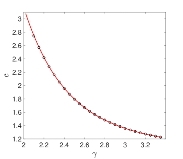
Figure 5: (Color online) The mean degree, $c=\langle K\rangle$, as a function of the exponent $\gamma$, for a configuration model network with a power-law degree distribution, where $k_{\rm min}=1$ and $k_{\rm max}=100$. As $\gamma$ is increased, the tail of the degree distribution decays more quickly and as a results the mean degree decreases. The analytical results (solid line) are found to be in excellent agreement with the results of computer simulations (circles) performed for networks of $N=4\times 10^{4}$ nodes.

In Fig. 5 we present analytical results for the mean degree $c=\langle K\rangle$ (solid line), of a configuration model network with a power-law degree distribution and $k_{\rm min}=1$, as a function of the exponent $\gamma$, for $\gamma>2$. As $\gamma$ is increased, the mean degree, $c$ decreases. The analytical results are in excellent agreement with the results of computer simulations (circles).

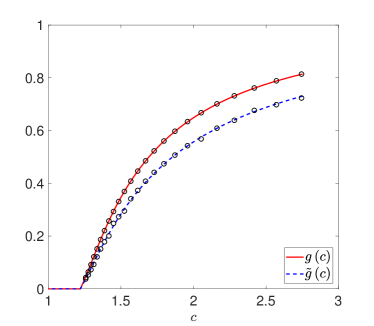
Figure 6: (Color online) Analytical results for the parameters $g$ (solid line) and $\tilde{g}$ (dashed line), as a function of the mean degree, $c$, for a configuration model network with a power-law degree distribution, where $k_{\rm min}=1$ and $k_{\rm max}=100$. The analytical results are found to be in excellent agreement with the results of computer simulations (circles), performed for networks of size $N=4\times 10^{4}$.

In Fig. 6 we present analytical results for the parameters $g$ (solid line) and $\tilde{g}$ (dashed line) for a configuration model network with a power-law degree distribution and $k_{\rm min}=1$, as a function of the mean degree, $c$. Below the percolation threshold there is no giant component and thus $g=\tilde{g}=0$. Above the percolation threshold both $g$ and $\tilde{g}$ gradually increase towards the dense limit result of $g=\tilde{g}=1$.

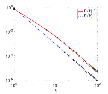
Figure 7: (Color online) Analytical results for the degree distribution $P(k|1)$ of the giant component of a configuration model network with a power-law degree distribution, where $\gamma=3$, $k_{\rm min}=1$ and $k_{\rm max}=100$ (solid line), obtained from Eq. (14), where $\tilde{g}$ and $g$ are obtained using the generating functions of Eqs. (100) and (101). The degree distribution $P(k)$ of the whole network (dashed line), obtained from Eq. (93), is also shown for comparison. The analytical results are found to be in excellent agreement with the results of computer simulations (circles), performed for networks of $N=4\times 10^{4}$ nodes,.

In Fig. 7 we present analytical results for the degree distribution $P(k|1)$ (solid line) of the giant component of a configuration model network with a power-law degree distribution where $k_{\rm min}=1$ and $\gamma=3$. For comparison, we also show the degree distribution $P(k)$ of the whole network (dashed line). The analytical results are in excellent agreement with the results of computer simulations (circles). Using Eq. (18), we calculate the mean degree on the giant component and obtain

$$\mathbb{E}[K|1]=\frac{\tilde{g}(2-\tilde{g})\left[\zeta(\gamma-1)-\zeta(\gamma-1,k_{\rm max}+1)\right]}{g\left[\zeta(\gamma)-\zeta(\gamma,k_{\rm max}+1)\right]}.$$ (102)

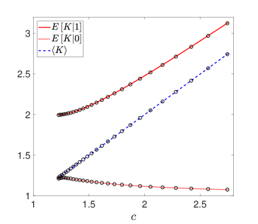
Figure 8: (Color online) Analytical results for the mean degree $\mathbb{E}[K|1]$ of the giant component (solid line) and the mean degree $\mathbb{E}[K|0]$ of the finite components (dotted line), as a function of $c$ above the percolation threshold, for a scale free configuration model network, where $k_{\rm min}=1$ and $k_{\rm max}=100$. The analytical results are found to be in excellent agreement with the results of computer simulations (circles), performed for networks of $N=4\times 10^{4}$ nodes. The mean degree $\langle K\rangle=c$ of the whole network (dashed line) is also shown for comparison.

In Fig. 8 we present analytical results for the mean degree, $\mathbb{E}[K|1]$, of the giant component (solid line) and the mean degree $\mathbb{E}[K|0]$, of the finite components (dotted line). The mean degree $\langle K\rangle$ of the whole network (dashed line) is also shown for comparison. The analytical results are in excellent agreement with the results of computer simulations.

Inserting the expression for $G_{1}(x)$ from Eq. (101) into Eqs. (47) and (48) we obtain the functions $B(u,v)$ and $S(u)$, respectively. Inserting them into Eq. (49) we obtain the assortativity coefficient $r$.

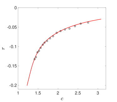
Figure 9: (Color online) The assortativity coefficient $r$ of the giant component of a configuration model network with a power-law degree distribution, with $k_{\rm min}=1$ and and $k_{\rm max}=100$, as a function of the mean degree, $c$. The analytical results (solid line) are found to be in very good agreement with the results of computer simulations (circles), performed for networks of $N=8\times 10^{4}$ nodes. The negative values of $r$ imply that the giant component is disassortative, namely high degree nodes preferentially connect to low degree nodes and vice versa. As $c$ is increased, the giant component encompasses an increasing fraction of the entire network, and $r$ decays to zero.

In Fig. 9 we present analytical results (solid line) for the assortativity coefficient $r$ of the giant component of a configuration model network with a power-law degree distribution, as a function of the mean degree, $c$. The analytical results are found to be in very good agreement with the results of computer simulations. For small values of $c$, just above the percolation threshold, the coefficient $r$ is large and negative. In this regime, the giant component encompasses only a small fraction of the network and is highly correlated. As $c$ is increased, the size of the giant component increases encompassing a larger fraction of the nodes in the network, and the assortativity coefficient gradually decays to zero. Using entropic considerations, one can show that negative degree-degree correlations are indeed typical in scale-free networks Johnson2010 ; Williams2014 .

VII Percolation on the giant component

Consider an ensemble of random networks of size $N$, with a given degree statistics, which can be characterized by a degree distribution, $P(k)$, degree-degree correlations and possibly higher order correlations. The probability of a random node to reside on the giant component is $g$, while the probability of a random neighbor of a random node to reside on the giant component is $\tilde{g}$. Thus, in the limit of $N\rightarrow\infty$, the size of the giant component is $gN$. Here we focus on the sub-network which consists of the giant component of the primary network. Clearly, this network consists of a single connected component. This property is reflected in the fact that taking the complete degree statistics of the primary network model and conditioning on its giant component, the probability, $\sigma$, that a random node will reside on the giant component must satisfy $\sigma=1$.

In what follows, we use generating functions to explore how well the result of $\sigma=1$ is reproduced, when degree statistics conditioned on the giant component is used in approximate ways. Following the classical percolation theory, as summarized by Eq. (7), the probability $\sigma$ satisfies

$$\sigma=\sum_{k}P(k|1)\left[1-(1-\tilde{\sigma})^{k}\right],$$ (103)

where $P(k|1)$ is the degree distribution conditioned on the giant component given by Eq. (14), and $\tilde{\sigma}$ is the probability that a randomly chosen edge points to a node connected to the giant component. Hence

$$\sigma=\frac{1}{g}\sum_{k}P(k)\left[1-(1-\tilde{g})^{k}\right]\left[1-(1-\tilde{\sigma})^{k}\right],$$ (104)

which can also be written in the form

$$\sigma=\frac{1}{g}\left[1-G_{0}(1-\tilde{g})-G_{0}(1-\tilde{\sigma})+G_{0}((1-\tilde{g})(1-\tilde{\sigma}))\right].$$ (105)

In order to utilize these equations, one should first calculate $\tilde{\sigma}$. This is done using an approximate self-consistency equation for $\tilde{\sigma}$. One can derive several variants for this equation, which depend on the level of detail in which the degree-degree correlations are taken into account. Below we present two such variants. In the first variant we account only for the degree distribution, $P(k|1)$, ignoring the degree-degree correlations. This variant resembles the self-consistency equation [Eq. (6)]. In the second variant we account for both the degree distribution and the correlations between the degrees of adjacent nodes.

VII.1 Configuration Model Approximation

We first consider the simplest approximation, in which the degree-degree correlations are ignored. In this case, the giant component is considered as a configuration model network with the degree distribution $P(k|1)$. In this approximation the self-consistency equation for $\tilde{\sigma}$ is given by

$$1-\tilde{\sigma}=\sum_{k}\frac{k}{c_{1}}P(k|1)(1-\tilde{\sigma})^{k-1},$$ (106)

where $P(k|1)$ given by Eq. (14) and $c_{1}$ is given by Eq. (18). This equation reflects the same reasoning as in Eq. (6). Inserting $P(k|1)$ and expressing the right hand side in terms of the generating functions, one obtains

$$1-\tilde{\sigma}=\frac{1}{1-(1-\tilde{g})^{2}}\left[G_{1}(1-\tilde{\sigma})-(1-\tilde{g})G_{1}((1-\tilde{g})(1-\tilde{\sigma}))\right].$$ (107)

VII.2 Approximation using degree-degree correlations

Taking degree-degree correlations into account as encoded in the degree distribution, $\widetilde{P}(k|1)$, of random neighbors of random nodes, given by Eq. (34), one obtains a self-consistency equation of the form

$$1-\tilde{\sigma}=\sum_{k}\widetilde{P}(k|1)(1-\tilde{\sigma})^{k-1},$$ (108)

or

$$1-\tilde{\sigma}=\frac{1}{g}\left\{(1-p_{0})G_{1}(1-\tilde{\rho})-\frac{1-g-p_{0}}{1-\tilde{g}}G_{1}[(1-\tilde{g})(1-\tilde{\sigma})]\right\}.$$ (109)

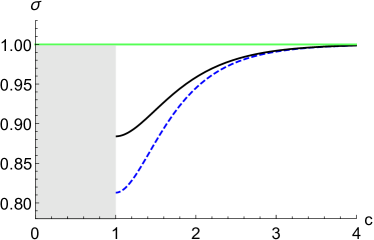
Figure 10: (Color online) The probability, $\sigma$, that a random node on the giant component of an ER network, will remain on the giant component in approximate self-consistent formulations, as a function of $c$. The results obtained by taking into account only the degree distribution, $P(k|1)$, are shown by a dashed line (blue), while the results obtained by adding the degree-degree correlations are shown by a solid line (black). It is found that the inclusion of degree-degree correlations significantly improves the results, bringing them closer to the exact result of $\sigma=1$ for $c>1$.

In Fig. 10 we present the fraction, $\sigma$, of nodes on the giant component of an ER network which are accounted for as giant component nodes by an approximate self-consistent approach, as a function of the mean degree $c$. The results were obtained from a simple self-consistent approach which takes into account only the degree distribution $P(k|1)$ (dashed line), and a more complete approach which includes both the degree distribution and degree-degree correlations (solid line). The inclusion of degree-degree correlations significantly improves the results, bringing them closer to the exact result of $\sigma=1$ for $c>1$. However, even with these correlation included the probability $\sigma$ is still determined to be lower than $1$; the discrepancy is largest at small $c$, though never larger than $12\%$. Our results imply that additional correlations play a role in keeping the giant component as a single connected component.

However, for small values of $c$ the probability $\sigma$ is still lower than $1$, which means that additional correlations play a role in keeping the giant component as a connected component.

VIII Applications

In what follows, we present several results that exploit the degree distributions and the joint degree distributions of higher orders obtained in Sec. III. This analysis elucidates both the power and limitations of this approach.

VIII.1 Distribution of shortest path lengths on the giant component

Consider a random node, $i$, in an ER network of $N$ nodes and mean degree $c=(N-1)p$. The remaining $N-1$ nodes are organized in shells, such that the $\ell$th shell consists of the nodes which are at a distance $\ell$ from the central node, $i$. The number of nodes in the $\ell$th shell is denoted by $n_{\ell}$, where $n_{0}=1$. The total number of nodes in the $(\ell+1)$th shell and all the outer shells beyond it is given by $N_{\ell}=\sum_{\ell^{\prime}=\ell+1}^{\infty}n_{\ell}$. Therefore, the number of nodes in the $\ell$th shell can be expressed by $n_{\ell}=N_{\ell-1}-N_{\ell}$. The approach we now present for the calculation of the DSPL is called the random shells approach (RSA) Katzav2015 . Within this approach $n_{\ell}$ satisfies the recursion equation $n_{\ell+1}=N_{\ell-1}[1-(1-p)^{n_{\ell}}]$, which can also be written in the form $N_{\ell+1}=N_{\ell}(1-p)^{N_{\ell-1}-N_{\ell}}$, where $N_{0}=N-1$ and $N_{1}=(N-1)(1-p)$. We denote the probability that the shortest path length from node $i$ to another random node in the network is larger than $\ell$ by $P(L>\ell)$. This probability is given by $P(L>\ell)=N_{\ell}/(N-1)$. Using this relation one obtains a recursion equation for the distribution of shortest path lengths (DSPL), which is expressed in the form of a tail distribution. It is given by

$$P(L>\ell+1)=P(L>\ell)(1-p)^{(N-1)[P(L>\ell-1)-P(L>\ell)]},$$ (110)

where $P(L>0)=1$ and $P(L>1)=1-p$. It is worth mentioning that the DSPL of an ER network can also be obtained using the random paths approach, which is based on the shortest paths between pairs of nodes rather than the shells around a single node Katzav2015 . The latter approach was extended to the case of configuration model networks Nitzan2016 ; Melnik2016 .

In the following, we will make an attempt at improving this approach based on the results derived for the giant component. In the classical RSA theory the reference node $i$ is considered as a ’typical’ node in the spirit of mean-field theory, and its degree is assumed to be equal to the mean degree, $c$. In practice, the degree of a random reference node is drawn from the degree distribution $P(k)$. Moreover, the degree of the reference node, $i$, has a strong effect on the shell structure around it. To account for this effect, we consider the shell structure around a node $i$ of a given degree $k_{0}$. In this case, $P(L=1|k_{0})=k_{0}/(N-1)$ and $P(L>1|k_{0})=1-k_{0}/(N-1)$. The recursion equations take the form

$$P(L>\ell+1|k_{0})=P(L>\ell|k_{0})\left(1-\frac{c}{N-1}\right)^{(N-1)P(L=\ell|k_{0})},$$ (111)

and

$$P(L=\ell+1|k_{0})=P(L>\ell|k_{0})-P(L>\ell+1|k_{0}).$$ (112)

Note that in case that $i$ is an isolated node, namely $k_{0}=0$, one obtains $P(L>\ell|k_{0}=0)=1$ for any values of $\ell$. The DSPL is then assembled from these conditional probabilities, with suitable weights, according to

$$P(L>\ell)=\sum_{k_{0}=0}^{\infty}P(k_{0})P(L>\ell|k_{0})$$ (113)

where

$$P(k_{0})=\frac{e^{-c}c^{k_{0}}}{k_{0}!}$$ (114)

is the Poisson distribution. Separating the case of $k_{0}=0$ we obtain

$$P(L>\ell)=e^{-c}+\sum_{k_{0}=1}^{\infty}\frac{e^{-c}c^{k_{0}}}{k_{0}!}P(L>\ell|k_{0}).$$ (115)

Since the analysis leading to Eq. (115) takes into account the effect of the degree, $k_{0}$, of the reference node, $i$, on the shell structure around it, this approach is referred to as the kRSA approach. We will now focus on the asymptotic tail of $P(L>\ell)$, which accounts for the fraction of nodes which are infinitely far away from $i$. On a finite network, the asymptotic value is given by $P(L>N-1)$. In this analysis we need to distinguish between the case in which $i$ resides on the giant component and the case in which it resides on one of the finite components. In case that $i$ is chosen randomly, without conditioning on its degree, the probability that it resides on the giant component is $P(\Lambda=1)=g$ and the probability that it resides on one of the finite components is $P(\Lambda=0)=1-g$. The degree distribution of nodes on the giant component is given by Eq. (52), while the degree distribution of nodes which reside on one of the finite components is

$$P(k|0)=e^{-c(1-g)}\frac{[c(1-g)]^{k}}{k!}.$$ (116)

For a node that resides on one of the finite components, we can approximate the DSPL by $P(L>\ell|\Lambda=0)=1$ for all values of $\ell>0$. This is an excellent approximation because the vast majority of pairs of nodes which are not on the giant component are not connected, since they do not belong to the same component at all. More precisely, the probability that they are connected scales as $1/N$ and hence negligible in the large network size limit. Under this assumption

$$P(L>\ell)=P(\Lambda=0)P(L>\ell|\Lambda=0)+P(\Lambda=1)\sum_{k_{0}=0}^{\infty}P(k_{0}|1)P(L>\ell|k_{0}),$$ (117)

or more explicitly

$$P(L>\ell)=(1-g)+\sum_{k_{0}=0}^{\infty}\frac{e^{-c}c^{k_{0}}}{k_{0}!}\left[1-e^{cg}(1-g)^{k_{0}+1}\right]P(L>\ell|k_{0}).$$ (118)

The analysis leading to Eq. (118) takes into account the distinction between reference nodes which reside on the giant component (with probability $g$) or on the non-giant components (with probability $1-g$), respectively. This analysis is thus referred to as the kgRSA approach.

To obtain the asymptotic value $P_{\infty}=P(d>N-1)$, we insert in Eq. (118) the identity $P(L>N-1|k_{0})=1-g$ for all values of $k_{0}$, since the $(1-g)N$ nodes which are not on the giant component are always beyond reach. In this case, the sum over the degree distribution in Eq. (118) is equal to $g$. Therefore,

$$P_{\infty}=(1-g)+g(1-g)=1-g^{2},$$ (119)

which coincides with the known exact result, namely with the probability that two random nodes do not reside simultaneously on the giant component.

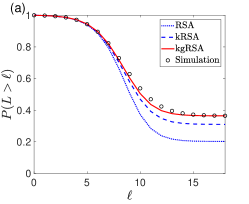
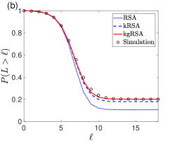
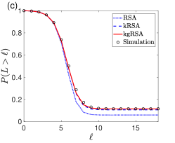
Figure 11: (Color online) Analytical results (dotted, dashed and solid lines) and simulation results (circles) for the tail distribution of the shortest path lengths, $P(L>\ell)$, of an ER network of $N=1000$ nodes with $c=2$ (a), $2.5$ (b) and $3$ (c). The RSA results (dotted lines), obtained from Eq. (110), are accurate for small distances but greatly under-estimate the tail distribution for large distances. The kRSA results (dashed lines), obtained from Eq. (115), which applies the overall degree distribution $P(k)$, provide a significant improvement, but are still too low. The kgRSA results (solid lines), obtained from Eq. (118), which takes into account the degree distribution on the giant component, $P(k|1)$, are found to be in very good agreement with the simulation results (circles).

In Fig. 11 we present analytical results (dotted, dashed and solid lines) and simulation results (circles) for the tail distribution $P(L>\ell)$ of an ER network of $N=1000$ nodes with $c=2$ (a), $2.5$ (b) and $3$ (c). The RSA results (dotted lines), obtained from Eq. (110), are accurate for small distances but greatly under-estimate the tail distribution for large distances. The kRSA results (dashed lines), obtained from Eq. (115), account for the degree of the central node and whether this node belongs (or not) to the giant component. This approach provides a significant improvement, but the resulting probabilities are still lower than the results of the simulations. The kgRSA results (solid lines), obtained from Eq. (118), account for the degree of the central node and are summed up using $P(k|1)$. These results are found to be in very good agreement with the simulation results (circles), and coincide with the tail exactly.

VIII.2 The spectra of the giant component

In this section we present an example of a problem in which the knowledge of the degree distributions on the giant component, $P(k|1)$ and $\widetilde{P}(k|1)$, enables to utilize a known formalism developed for the entire network, for the analysis of the giant component alone. There are many problems in which this approach can be applied, by replacing the degree distributions of the entire network, $P(k)$ and $\widetilde{P}(k)$, by the corresponding degree distributions conditioned on the giant component, $P(k|1)$ and $\widetilde{P}(k|1)$, in the equations which provide the desired properties.

The specific example we consider involves the the calculation of the spectra of the adjacency matrices of configuration model networks, using methods of random matrix theory Mehta2004 ; Livan2018 . The methodology for studying the spectrum of the adjacency matrix, $A$, of an entire network was developed in Refs. Kuhn2008 ; Rogers2008 . It is based on a representation of the spectral density of a matrix $A$ in terms of the trace of its resolvent

$$\rho(\lambda)=\frac{1}{\pi N}\lim_{\epsilon\rightarrow 0^{+}}{\rm Im}{\rm Tr}(\lambda_{\epsilon}I-A)^{-1},$$ (120)

where $I$ is the identity matrix and $\lambda_{\epsilon}=\lambda-i\epsilon$. In fact, Eq. (120) is an example of the Stieltjes-Peron inversion formula Akhiezer1965 . Edwards and Jones Edwards1976 expressed the trace of the resolvent in terms of a sum over single-site variances

$$\rho(\lambda)=\frac{1}{\pi N}{\rm Re}\sum_{i}\langle u_{i}^{2}\rangle,$$ (121)

of the complex Gaussian measure

$$p({\bf u})=\frac{1}{Z}\,{\rm e}^{{\rm i}H({\bf u})}$$ (122)

in which $H({\bf u})$ is given by the quadratic form

$$H({\bf u})=\frac{1}{2}\sum_{i,j}(\lambda_{\epsilon}\delta_{ij}-A_{ij})u_{i}u_{j}.$$ (123)

The formalism of Refs. Kuhn2008 ; Rogers2008 ; Kuhn2016 enables one to express the ensemble average of $\rho(\lambda)$ in terms of the distribution $\pi(\omega)$ of so-called inverse single-cavity variances corresponding to the multi-variate complex Gaussian (122). It takes the form

$$\rho(\lambda)=\frac{1}{\pi}{\rm Re}\sum_{k\geq 0}P(k)\int\prod_{\nu=1}^{k}d\pi(\omega_{\nu})\frac{1}{i\lambda_{\epsilon}+\sum_{\nu=1}^{k}\frac{1}{\omega_{\nu}}}.$$ (124)

The distribution $\pi(\omega)$ of inverse single-cavity variances is determined as solution of the self-consistency equation

$$\pi(\omega)=\sum_{k\geq 1}\widetilde{P}(k)\int\prod_{\nu=1}^{k-1}d\pi(\omega_{\nu})\delta\left(\omega-i\lambda_{\epsilon}-\sum_{\nu=1}^{k-1}\frac{1}{\omega_{\nu}}\right).$$ (125)

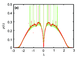
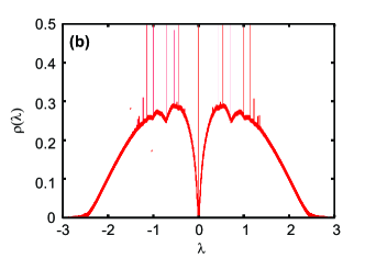
Figure 12: (Color online) (a) The spectrum of the adjacency matrix of the giant component of an ER network of mean degree $c=2$ (red solid line), compared with an approximation that takes degree-degree correlations at the level of Eq. (39) into account (green dashed line). The approximate description does not exclude the existence of finite components (as can be seen in Fig. 10), so has more weight in localized states with support on finite components (represented by $\delta$-peaks in the spectrum); (b) The exact spectrum shown separately, demonstrating that the exact spectrum of the giant component also exhibits a number of localized states (corresponding to sub-graph configurations with $\mathbb{Z}_{2}$ symmetry).

In this work we adapt the ensemble averaging step in the formalism reviewed above to reflect the degree distributions and degree-degree correlations on the giant component. This amounts to replacing $P(k)$ in Eq. (124) by $P(k|1)$ and replacing $\widetilde{P}(k)$ in Eq. (125) by $\widetilde{P}(k|1)$ [Eq. (34)]. We apply this approach to the calculation of the spectrum of the adjacency matrices, conditioned on the giant component, for an ensemble of ER networks with $c=2$ in the large $N$ limit. In Fig. 12 we present the resulting spectrum (solid line), compared with an approximation that takes degree-degree correlations at the level of Eq. (34) into account (dashed line). The approximate description does not exclude the existence of finite components (as seen in section VII B), so has more weight in localized states with support on finite components (represented by $\delta$-peaks). We also show separately the exact spectrum calculated using the approach of Ref. Kuhn2016 , demonstrating that the exact spectrum of the giant component also exhibits a number of localized states (corresponding to sub-graph configurations with $\mathbb{Z}_{2}$ symmetry).

VIII.3 Epidemic spreading on the giant component

One of the most important dynamical processes taking place on networks is the spreading or propagation of infections, information and opinions. To discuss processes of epidemic spreading on a network, let us first define the possible states of a node as susceptible (S), infected (I) or recovered (R) Karrer2010 ; Rogers2015 ; Satorras2015 . The transitions between these states include, for example, S $\rightarrow$ I, where a susceptible node becomes infected due to the interaction with an infected neighbor. In the susceptible-infected-susceptible (SIS) model, the infected node later recovers and returns to the S state, while in the susceptible-infected-recovered (SIR) model, the infected node recovers and becomes immune to further infections. The classical epidemic models have been studied extensively leading to many insights and applications such as assessment of vaccination strategies.

The infection is considered as a stochastic process, starting from a random infected node, and propagates through the network. Each infected node infects each of its neighbors with probability $\rho$. In each instance of this process, the number of infected nodes exhibits temporal fluctuations until the infection dies out. The statistical properties of the infections depend on the network structure and on the parameter $\rho$. The long term dynamics of an SIR model on a network can be mapped into a bond percolation problem on the network Karrer2010 . The percolation problem involves a random deletion of edges, such that each edge in the network is maintained with probability $\rho$ and deleted with probability $1-\rho$. Within this construction, the probability, $\sigma$, of a random node in a configuration model network to remain on the giant component corresponds to the fraction of the individuals which have become infected. This fraction is given by

$$\sigma=1-\sum_{k=0}^{\infty}P(k)(1-\rho\tilde{\sigma})^{k}=1-G_{0}(1-\rho\tilde{\sigma}),$$ (126)

where $\tilde{\sigma}$ is the probability that a random neighbour of a random node is a part of the giant component, which satisfies the self-consistency equation

$$\tilde{\sigma}=1-\sum_{k}\frac{k}{c}P(k)(1-\rho\tilde{\sigma})^{k-1}=1-G_{1}(1-\rho\tilde{\sigma}).$$ (127)

These equations closely resemble those used to identify the fraction of nodes in the giant component of the primary network discussed above in section VII. We can now apply some of the heuristics developed in this work to recover aspects of heterogeneity in the percolation problem on random networks that were recently described in Kuhn2017 , without having to apply the message passing and population dynamics techniques used in that paper.

As in Sec. VII we rewrite the equation for $\sigma$ in a manner that allows us to explore its probabilistic content, by iteratively inserting the self-consistency equation (127) for $\tilde{\sigma}$. In order to achieve more compact versions for the resulting expression we choose to rewrite Eq. (127) as an equation for the variable $\tilde{h}\equiv 1-\rho\tilde{\sigma}$, giving

$$\tilde{h}=1-\rho\left[1-G_{1}(\tilde{h})\right]=\sum_{k}\frac{k}{c}P(k)\left[1-\rho(1-\tilde{h}^{k-1})\right].$$ (128)

To first order, we obtain

$$\sigma=\sum_{k=0}^{\infty}P(k)\left(1-\tilde{h}^{k}\right).$$ (129)

Replacing $\tilde{h}$ in Eq. (129) by the right hand side of Eq. (128), we obtain

$$\sigma=\sum_{k;\{k_{\mu}\}}P(k)\prod_{\mu=1}^{k}\frac{k_{\mu}}{c}P(k_{\mu})\left[1-\prod_{\mu=1}^{k}\left(1-\rho(1-\tilde{h}^{k_{\mu}-1})\right)\right].$$ (130)

Repeating this procedure once again we obtain

$$\sigma = \sum_{k;\{k_{\mu}\};\{k_{\mu\nu}\}}P(k)\prod_{\mu=1}^{k}\frac{k_{\mu}}{c}P(k_{\mu})\prod_{\nu=1}^{k_{\mu}-1}\frac{k_{\mu\nu}}{c}P({k_{\mu\nu}})\times$$ (131)

$$\left[1-\prod_{\mu=1}^{k}\left(1-\rho\left(1-\prod_{\nu=1}^{k_{\mu}-1}\left(1-\rho(1-\tilde{h}^{k_{\mu\nu}-1})\right)\right)\right)\right],$$

and so on. Following the reasoning of Sec. IV we can use these equations to identify a string of conditional probabilities of infection of a node, given its degree and the degree configurations of its first and second coordination shells, and of further configuration shells if the above iterative process were indeed continued.

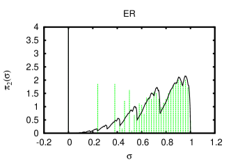
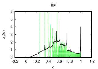
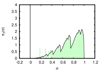
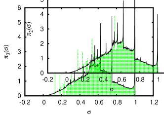
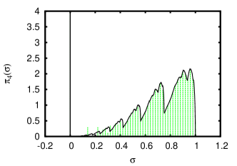
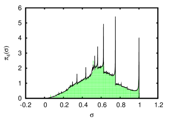
Figure 13: (Color online) Approximate evaluations of the heterogeneous infection probabilities $\pi_{2}(\sigma)$, $\pi_{3}(\sigma)$ and $\pi_{4}(\sigma)$ (top to bottom) represented by green dashed histograms, for an ER network with $c=2$ (left column) and a configuration model network (right column) with a power-law degree distribution of the form $P(k)\sim k^{-\gamma}$ with $\gamma=3$ and $k_{\rm min}=2$, also referred to as a scale-free (SF) network. Also shown in each panel is the full distribution $\pi(\sigma)$ (black solid line) obtained using a population dynamics approach to solving the self-consistency equations arising in this problem. While the low order approximations are reasonable at the large $\sigma$ end, higher order approximations taking degree configurations of higher order coordination shells into account are needed to improve accuracy at the small $\sigma$ end of the probability distribution function.

Interestingly, these results allow us to obtain increasingly accurate approximations of the full probability density function $\pi(\sigma)$ of the heterogeneous infection/percolation probabilities defined and evaluated in Ref. Kuhn2017 . In particular, with reference to Eqs. (129)-(131), we define approximations of increasing orders for $\pi(\sigma)$, starting from the lowest order expression of the form

$$\pi_{0}(\sigma)=\sum_{k}P(k)\,\delta\left[\sigma-(1-\tilde{h}^{k})\right].$$ (132)

Replacing $\tilde{h}$ in Eq. (132) by the right hand side of Eq. (128), we obtain

$$\pi_{1}(\sigma)=\sum_{k;\{k_{\mu}\}}P(k)\prod_{\mu=1}^{k}\frac{k_{\mu}}{c}P(k_{\mu})\delta\left[\sigma-\left(1-\prod_{\mu=1}^{k}\left(1-\rho(1-\tilde{h}^{k_{\mu}-1})\right)\right)\right].$$ (133)

Repeating this procedure once more we obtain

$$\pi_{2}(\sigma) = \sum_{k;\{k_{\mu}\};\{k_{\mu\nu}\}}P(k)\prod_{\mu=1}^{k}\frac{k_{\mu}}{c}P(k_{\mu})\prod_{\nu=1}^{k_{\mu}-1}\frac{k_{\mu\nu}}{c}P(k_{\mu\nu})\times$$ (134)

$$\delta\left[\sigma-\left(1-\prod_{\mu=1}^{k}\left(1-\rho\left(1-\prod_{\nu=1}^{k_{\mu}-1}\left(1-\rho(1-\tilde{h}^{k_{\mu\nu}-1})\right)\right)\right)\right)\right],$$

and so on. We note that each of these approximate probability density functions of the heterogeneous percolation probabilities reproduces the same (exact) average percolation probability $\sigma$, as can easily be checked by evaluating the averages, and using the iterated expressions of Eqs. (129)-(131) for $\sigma$.

In Fig. 13 we show evaluations of $\pi_{2}(\sigma)$, $\pi_{3}(\sigma)$ and $\pi_{4}(\sigma)$ for an ER network with mean degree of $c=2$, with transmission probability (bond occupation probability) $\rho=0.75$, and for a scale free graph with $P(k)\sim k^{-3}$ and $k_{\rm min}=2$, with a transmission probability $\rho=0.5$. From the full distribution $\pi(\sigma)$ and in particular from its deconvolution according to the degrees of the central node, one can conclude that long dangling chain configurations (with few side-branches) are mainly responsible for the small-$\sigma$ features of $\pi(\sigma)$, and to describe sufficiently long chains of this type one would have to include higher-order coordination shells in the analysis. But the trend towards a reasonably precise description of $\pi(\sigma)$ using these low order approximations is clearly visible. Given that the present approach is clearly both conceptually and computationally ‘low-tech’ compared with the full theory exploited in Kuhn2017 , the present low order approximation manage to accurately reproduce a considerable amount of detail of these highly non-trivial distributions. For the purpose of the evaluation of the approximations, we used sampling from randomly generated degree configurations up to the highest order configuration shell involved rather than a full evaluation of the sums appearing in Eqs. (132)-(134), as well as the equations for $\pi_{3}(\sigma)$ and $\pi_{4}(\sigma)$ which are not displayed above.

IX Summary and Discussion

We have studied the micro-structures of the giant component and the finite components of configuration model networks. We found that the finite components form a sub-percolating configuration model network with a modified degree distribution. In particular, the degree distribution of the finite components is simply an exponentially attenuated version of the original degree distribution of the network [Eq. (16)]. We recovered the known result for the self duality of the ER network Molloy1995 ; Bollobas2001 . This self duality means that the finite components of an ER network with $c>1$ form a sub-percolating ER network with mean degree $c_{0}=(1-g)c<1$. Moreover, we extended this result to a broad class of configuration model networks. This includes the configuration model with an exponential degree distribution and the configuration model with a power-law degree distribution and an exponential cutoff.

In contrast, we found that the giant component of a configuration model network is not itself a configuration model network. In fact, it exhibits degree-degree correlations to all orders, as exemplified by our analysis of the percolation problem on the giant component, the spectrum of the giant component and the DSPL on the giant component. We presented analytical results for the degree distribution on the giant component as well as the joint degree distribution of pairs of adjacent nodes. Furthermore, we provided a methodology for the derivation of the joint degree distribution of a random node together with several shells around it. We derived an expression for the assortativity coefficient of the giant component. Interestingly, the giant component was found to be disassortative, namely high degree nodes tend to connect preferentially to low degree nodes. This can be understood intuitively due to the fact that disassortativity helps to maintain the integrity of the giant component. In contrast, the segregation between high degree nodes and low degree nodes would fragment the giant component into small pieces. In general, we found that as the network approaches the percolation transition from above and the giant component decreases in size, its structure becomes more distinct from the structure of the overall network. In particular, the degree distribution deviates more strongly from the overall degree distribution, the degree-degree correlations become stronger and the assortativity coefficient becomes more negative.

The results presented in this paper have broad implications for dynamical processes on configuration model networks. For example, epidemic processes are most consequential when they occur on the giant component. If an epidemic starts on a node which resides on a finite component it quickly terminates after infecting a small, non-extensive, number of nodes. In contrast, an epidemic which starts on a node which resides on the giant component endangers a significant fraction of the entire network. Therefore, the quantities of interest in the context of epidemics (as well as many other dynamical processes) are those that characterize the giant component rather than the overall network. The examples discussed in this paper demonstrate the difference between the properties which are conditioned on the giant component and the corresponding properties of the entire network.

Our results for the degree distribution and the degree-degree correlations on the giant component provide a practical and straightforward way to calculate the properties of many dynamical processes conditioned on the giant component. Such processes include information spreading, search processes, network attacks and random walks. This can be done by utilizing existing theoretical formulations which were derived for configuration model networks and replacing the degree distribution of the overall network by the degree distribution conditioned on the giant component. A more complete formulation can be obtained by incorporating joint degree distributions, which capture the degree-degree correlations. The examples discussed in this paper show that adapting existing theoretical formulations to account for the special properties of the giant component provide better approximations than those obtained using the corresponding properties of the overall network.

References

- (1) R. Albert and A.-L. Barabási, Statistical mechanics of complex networks, Rev. Mod. Phys. 74 47-97 (2002).
- (2) S.N. Dorogovtsev and J.F.F. Mendes, Evolution of networks: from biological networks to the internet and WWW (Oxford University Press, Oxford, 2003).
- (3) S.N. Dorogovtsev, A.V. Goltsev and J.F.F. Mendes, Critical phenomena in complex networks, Rev. Mod. Phys. 80, 1275-1335 (2008).
- (4) R. van der Hofstad, Random Graphs and Complex Networks, Vol. 1 (Cambridge University Press, 2016).
- (5) M.E.J. Newman, Networks: an introduction (Oxford University Press, Oxford, 2010).
- (6) A. Barrat, M. Barthélemy and A. Vespignani, Dynamical processes on complex networks (Cambridge University Press, Cambridge, 2012).
- (7) P. Erdős and Rényi, On random graphs I, Publicationes Mathematicae Debrecen 6, 290-297 (1959).
- (8) P. Erdős and Rényi, On the evolution of random graphs, Publ. Math. Inst. Hung. Acad. Sci. 5, 17-61 (1960).
- (9) P. Erdős and Rényi, On the evolution of random graphs II, Bull. Int. Stat. Inst. 38, 343-347 (1961).
- (10) B. Bollobás, The evolution of random graphs, Trans. Amer. Math. Soc. 286, 257-274 (1984).
- (11) M. Molloy and A. Reed, A critical point for random graphs with a given degree sequence, Random Structures and Algorithms 6, 161-180 (1995).
- (12) M. Molloy and A. Reed, The size of the giant component of a random graph with a given degree sequence, Combin., Prob. and Comp. 7, 295-305 (1998).
- (13) B. Bollobás, Random graphs (Cambridge University Press, Cambridge, 2001).
- (14) B. Bollobás, S. Janson and O. Riordan, The phase transition in inhomogeneous random graphs, Random Structures & Algorithms 31, 3-122 (2007).
- (15) S. Janson and O. Riordan, Duality in inhomogeneous random graphs, and the cut metric, Random Structures & Algorithms 39, 399-411 (2011).
- (16) A. Engel, R. Monasson and A.K. Hartmann, On large-deviation properties of Erdős-Rényi random graphs, J. Stat. Phys. 117, 387-425, (2004).
- (17) G. Biroli and R. Monasson, A single defect approximation for localized states on random lattices, J. Phys. A 32, L255-L261 (1999).
- (18) R. Kühn, Spectra of sparse random matrices, J. Phys. A 41, 295002 (2008).
- (19) V. Sood, S. Redner and D. ben-Avraham, First-passage properties of the Erdős-Rényi random graph, J. Phys. A 38, 109 (2005).
- (20) C. De Bacco, S. N. Majumdar and P. Sollich, The average number of distinct sites visited by a random walker on random graphs, J. Phys. A 48, 205004 (2015).
- (21) I. Tishby, O. Biham and E. Katzav, The distribution of path lengths of self avoiding walks on Erdős-Rényi networks, J. Phys. A 49, 285002 (2016).
- (22) I. Tishby, O. Biham and E. Katzav, The distribution of first hitting times of randomwalks on Erdős-Rényi networks, J. Phys. A 50, 115001 (2017).
- (23) D.J. Watts, A simple model of global cascades on random networks, Proc. Natl. Acad. Sci. USA 99, 5766-5771 (2002).
- (24) M.E.J. Newman, Spread of epidemic disease on networks, Phys. Rev. E 66, 016128 (2002).
- (25) M.E.J. Newman, Assortative mixing in networks, Phys. Rev. Lett. 89, 208701 (2002).
- (26) B. Karrer and M. E. J.Newman, Message passing approach for general epidemic models, Phys. Rev. E 82, 016101 (2010).
- (27) T. Rogers, Assessing node risk and vulnerability in epidemics on networks, Europhys. Lett. 109, 28005 (2015).
- (28) R. Pastor-Satorras, C. Castellano, P. Van Mieghem, and A. Vespignani, Epidemic processes in complex networks, Rev. Mod. Phys. 87, 925-979 (2015).
- (29) D.S. Callaway, M.E.J. Newman, S.H. Strogatz and D.J. Watts, Network robustness and fragility: percolation on random graphs, Phys. Rev. Lett. 85, 5468-5471 (2000).
- (30) V.D. Blondel, J.-L. Guillaume, J. M. Hendrickx and R.M. Jungers, distance distribution in random graphs and application to network exploration, Phys. Rev. E 76, 066101 (2007).
- (31) E. Katzav, M. Nitzan, D. ben Avraham, P. L. Krapivsky, R. Kühn, N. Ross and O. Biham, Analytical results for the distribution of shortest path lengths in random networks, EPL 111, 26006 (2015).
- (32) M. Nitzan, E. Katzav, R. Kühn and O. Biham, Distance distribution in configuration-model networks, Phys. Rev. E 93, 062309 (2016).
- (33) S. Melnik and J.P. Gleeson, Simple and accurate analytical calculation of shortest path lengths, arXiv:1604.05521 (2016).
- (34) M.E.J. Newman, S.H. Strogatz and D.J. Watts, Random graphs with arbitrary degree distributions and their applications, Phys. Rev. E 64, 026118 (2001).
- (35) P. Erdős and T. Gallai, Graphs with given degrees of vertices, Matematikai Lapok 11, 264-274 (1960).
- (36) S.A. Choudum, A simple proof of the Erdős-Gallai theorem on graph sequences, Bulletin of the Australian Mathematical Society 33, 67-70 (1986).
- (37) F.W.J. Olver, D.M. Lozier, R.F. Boisvert and C.W. Clark, NIST handbook of mathematical functions (Cambridge University Press, Cambridge, 2010).
- (38) H. Bonneau , A. Hassid, O. Biham, R. Kühn and E. Katzav, Distribution of shortest cycle lengths in random networks, Phys. Rev. E 96, 062307 (2017).
- (39) L.A. Shepp and S.P. Lloyd, Ordered Cycle Lengths in a Random Permutation, Transactions American Math. Soc. 121, 340-357 (1966).
- (40) S. Johnson, J.J. Torres, J. Marro, and M.A. Muñoz, Entropic origin of disassortativity in complex networks, Phys. Rev. Lett. 104, 108702 (2010).
- (41) O. Williams and C.I. Del Genio, Degree correlations in directed scale-free networks, PLoS ONE 9, e110121 (2014).
- (42) M.L. Mehta, Random matrices (Academic Press, Amsterdam, 2004).
- (43) G. Livan, M. Novaes and P. Vivo, Introduction to random matrices: theory and practice (Springer International Publishing, Cham, 2018).
- (44) T. Rogers, I. Pérez Castillo, R. Kühn and K. Takeda, Cavity approach to the spectral density of sparse Symmetric Random Matrices, Phys. Rev. E 78, 031116 (2008).
- (45) N.I. Akhiezer, The classical moment problem and some related questions in analysis (Oliver & Boyd, Edinburgh, 1965).
- (46) S.F. Edwards and R.C. Jones, The eigenvalue spectrum of a large symmetric random matrix, J. Phys. A 9, 1595-1604 (1976).
- (47) R. Kühn, Disentangling giant component and finite cluster Contributions in Sparse Matrix Spectra, Phys. Rev. E 93, 042110 (2016).
- (48) R. Kühn and T. Rogers, Heterogeneous micro-structure of percolation in sparse networks, EPL 118, 68003 (2017).