Mean Field Network based Graph Refinement with application to Airway Tree Extraction

Abstract

We present tree extraction in 3D images as a graph refinement task, of obtaining a subgraph from an over-complete input graph. To this end, we formulate an approximate Bayesian inference framework on undirected graphs using mean field approximation (MFA). Mean field networks are used for inference based on the interpretation that iterations of MFA can be seen as feed-forward operations in a neural network. This allows us to learn the model parameters from training data using back-propagation algorithm. We demonstrate usefulness of the model to extract airway trees from 3D chest CT data. We first obtain probability images using a voxel classifier that distinguishes airways from background and use Bayesian smoothing to model individual airway branches. This yields us joint Gaussian density estimates of position, orientation and scale as node features of the input graph. Performance of the method is compared with two methods: the first uses probability images from a trained voxel classifier with region growing, which is similar to one of the best performing methods at EXACT’09 airway challenge, and the second method is based on Bayesian smoothing on these probability images. Using centerline distance as error measure the presented method shows significant improvement compared to these two methods.

1 Introduction

Markov random field (MRF) based image segmentation methods have been successfully used in several medical image applications [2, 10]. Pixel-level MRF’s are commonly used for segmentation purposes to exploit the regular grid nature of images. These models become prohibitively expensive when dealing with 3D images, which are commonly encountered in medical image analysis. However, there are classes of methods that work with supervoxel representation to reduce density of voxels by abstracting local information as node features [3, 11]. Image segmentation, in such models, can be interpreted as connecting voxels/supervoxels to extract the desired structures of interest. This has similarities with performing graph refinement, where an over-complete input graph is processed to obtain a subgraph that corresponds to structures of interest.

In this work, we present a novel approach to tree extraction by formulating it as a graph refinement procedure on MRF using mean field networks (MFN). We recover a subgraph corresponding to the desired tree structure from an over-complete input graph either by retaining or removing edges between pairs of nodes. We use supervoxel-like representation to associate nodes in the graph with features that make the input graph sparser. We formulate a probabilistic model based on unary and pairwise potential functions that capture nodes and their interactions. The inference is performed using mean field networks which implement mean field approximation (MFA) [1] iterations as feed-forward operation in a neural network [9]. The MFN interpretation enables us to learn the model parameters from training data using back-propagation algorithm; this allows our model to be seen as an intermediate between entirely model-based and end-to-end learning based approaches. The proposed model is exploratory in nature and, hence, not sensitive to local anomalies in data. We evaluate the method to extract airway trees in comparison with two methods: the first uses probability images from a trained voxel classifier with region growing [6], which is similar to one of the best performing methods in EXACT airway challenge [7], and the second method is based on Bayesian smoothing on probability images obtained from the voxel classifier [11].

2 Method

2.1 The Graph Refinement Model

Given a fully connected, or over-complete, input graph, ${\mathcal{G}}:\{{\mathcal{N}},{\mathcal{E}}\}$ with nodes $i\in{\mathcal{N}}$ and edges in $(i,j)\in{\mathcal{E}}$, we are interested in obtaining a subgraph, ${{\mathcal{G}}^{\prime}}:\{{\mathcal{N}}^{\prime},{\mathcal{E}}^{\prime}\}$, that in turn corresponds to a structure of interest like vessels or airways in an image. We assume each node $i\in{\mathcal{N}}$ to be associated with a set of $d$-dimensional features, ${\mathbf{x}}_{i}\in{\mathbb{R}}^{d}$, and collected into a random vector, ${\mathbf{X}}=[{\mathbf{x}}_{1},\dots,{\mathbf{x}}_{N}]$. We introduce a random variable, ${\mathbf{S}}=[{\mathbf{s}}_{1}\dots\mathbf{s}_{N}]$, to capture edge connections between nodes. Each node connectivity variable, ${\mathbf{s}}_{i}=\{s_{ij}\}:j=1\dots N$, is a collection of binary random variables, $s_{ij}\in\{0,1\}$, indicating absence or presence of an edge between nodes $i$ and $j$ and we are interested in recovering ${\mathbf{S}}^{\prime}$ that describes the desired subgraph ${\mathcal{G}}^{\prime}$. Note that each instance of ${\mathbf{S}}$ can be seen as an $N\times N$ adjacency matrix.

The model described by the conditional distribution, $p({\mathbf{S}}|{\mathbf{X}})$, bears similarities with hidden MRF models that have been used for image segmentation[2, 10]. Based on this connection, we use the notion of node, $\phi_{i}({\mathbf{s}}_{i})$, and pairwise, $\phi_{ij}({\mathbf{s}}_{i},{\mathbf{s}}_{j})$, potentials to write the logarithm of joint distribution and relate it to the conditional distribution as,

$$\ln p({\mathbf{S}}|{\mathbf{X}})\propto\ln p({\mathbf{S}},{\mathbf{X}})=-\ln Z+\sum_{i\in{\mathcal{N}}}\phi_{i}({\mathbf{s}}_{i})+\sum_{(i,j)\in{\mathcal{E}}}\phi_{ij}({\mathbf{s}}_{i},{\mathbf{s}}_{j}),$$ (1)

where $\ln Z$ is the normalisation constant. For ease of notation, explicit dependence on observed data in these potentials is not shown.

Next we focus on formulating node and pairwise potentials introduced in (1) to reflect the behaviour of nodes and their interactions in the subgraph ${\mathcal{G}}^{\prime}$, which can consequently yield good estimates of $p({\mathbf{S}}|{\mathbf{X}})$. First, we propose a node potential that imposes a prior degree on each node and learns a per-node feature representation that can be relevant to nodes in the underlying subgraph, ${\mathcal{G}}^{\prime}$. For each node $i\in{\mathcal{N}}$, it is given as,

$$\phi_{i}({\mathbf{s}}_{i})=\sum_{v=0}^{D}\beta_{v}{\mathbb{I}}\Big{[}\sum_{j}s_{ij}=v\Big{]}+{\mathbf{a}}^{T}{\mathbf{x}}_{i}\sum_{j}s_{ij},$$ (2)

where $\sum_{j}s_{ij}$ is the degree of node $i$ and ${\mathbb{I}}[\cdot]$ is the indicator function. The parameters $\beta_{v}\in{\mathbb{R}},\text{ }\forall\text{ }v=[0,\dots,D]$, can be seen as a prior on the degree per node. We explicitly model and learn this term for upto 2 edges per node and assume uniform prior for $D>2$. Further, individual node features, ${\mathbf{x}}_{i}$, are combined with ${\mathbf{a}}\in{\mathbb{R}}^{d\times 1}$ and captures a combined node feature representation that is characteristic to the desired subgraph ${\mathcal{G}}^{\prime}$. The degree of each node, $\sum_{j}s_{ij}$, controls the extent of each node’s contribution to the node potential.

Secondly, we model the pairwise potential such that it captures interactions between pairs of nodes and is crucial in deciding the existence of edges between nodes. We propose a potential that enforces symmetry in connections, and also has terms that derive joint features for each pair of nodes that are relevant in prediction of edges, and is given as,

$$\phi_{ij}({\mathbf{s}}_{i},{\mathbf{s}}_{j})=\lambda\big{(}1-2|s_{ij}-s_{ji}|\big{)}+(2s_{ij}s_{ji}-1)\Big{[}\boldsymbol{\eta}^{T}|{\mathbf{x}}_{i}-{\mathbf{x}}_{j}|+\boldsymbol{\nu}^{T}({\mathbf{x}}_{i}{\mathbf{x}}_{j})\Big{]}.$$ (3)

The function parameterised by $\lambda\in{\mathbb{R}}$ in (3) ensures symmetry in connections between nodes, i.e, for nodes $i,j$ it encourages $s_{ij}=s_{ji}$. The parameter $\boldsymbol{\eta}\in{\mathbb{R}}^{d\times 1}$ combines the absolute difference between each feature dimension. The element-wise feature product term $({\mathbf{x}}_{i}{\mathbf{x}}_{j})$ with $\boldsymbol{\nu}\in{\mathbb{R}}^{d\times 1}$ is a weighted, non-stationary polynomial kernel of degree 1 that computes the dot product of node features in a weighted feature space.

Under these assumptions, the posterior distribution, $p({\mathbf{S}}|{\mathbf{X}})$, can be used to extract the subgraph, ${{\mathcal{G}}^{\prime}}$ from ${\mathcal{G}}$. However, except for in trivial cases, it is intractable to estimate $p({\mathbf{S}}|{\mathbf{X}})$ and we must resort to making some approximations. We take up the variational mean field approximation (MFA) [1], which is a structured approach to approximating $p({\mathbf{S}}|{\mathbf{X}})$ with candidates from a class of simpler distributions$:q({\mathbf{S}})\in{\mathcal{Q}}$. This approximation is performed by minimizing the exclusive Kullback-Leibler divergence [1], or equivalently maximising the evidence lower bound (ELBO) or variational free energy, given as

$${\mathcal{F}}(q_{\mathbf{S}})=\ln Z+{\mathbb{E}}_{q_{{\mathbf{S}}}}\Big{[}\ln p({\mathbf{S}}|{\mathbf{X}})-\ln q({\mathbf{S}})\Big{]},$$ (4)

where ${\mathbb{E}}_{q_{{\mathbf{S}}}}$ is the expectation with respect to the distribution ${q_{{\mathbf{S}}}}$. In MFA, the class of distributions, ${\mathcal{Q}}$, are constrained such that $q({\mathbf{S}})$ can be factored further. In our model, we assume the existence of each edge is independent of the others, which is enforced as the following factorisation:

$$q({\mathbf{S}})=\prod_{i=1}^{N}\prod_{j=1}^{N}q_{ij}(s_{ij}),\text{ where }q_{ij}(s_{ij})=\begin{cases}\alpha_{ij}&\qquad\text{if }s_{ij}=1\\ (1-\alpha_{ij})&\qquad\text{if }s_{ij}=0\end{cases},$$ (5)

where $\alpha_{ij}\in[0,1]$ is the probability of an edge existing between nodes $i$ and $j$.

Using the potentials from (2) and (3) in (4) and taking expectation with respect to the distribution $q_{\mathbf{S}}$, we obtain the ELBO in terms of $\alpha_{ij}\text{ }\forall\text{ }i,j=[1,\dots,N]$, proof of which is shown in the Appendix 5. By differentiating this ELBO with respect to any individual $\alpha_{kl}$, we obtain the following update equation for performing MFA iterations. At iteration $(t+1)$:

$$\alpha_{kl}^{(t+1)}=\sigma({\gamma_{kl}})=\frac{1}{1+\exp^{-\gamma_{kl}}}\text{ }\forall\text{ }{k}=\{1\dots N\},\text{ }l\in{\mathcal{N}}_{k}\text{ }:\text{ }|{\mathcal{N}}_{k}|=L$$ (6)

where $\sigma(\cdot)$ is the sigmoid activation function, ${\mathcal{N}}_{k}$ are the $L$ nearest neighbours of node $k$ based on positional Euclidean distance, and

$$\gamma_{kl}=\prod_{j\in{\mathcal{N}}_{k}\setminus l}\big{(}1-\alpha_{kj}^{(t)}\big{)}\Big{\{}\sum_{m\in{\mathcal{N}}_{k}\setminus l}\frac{\alpha_{km}^{(t)}}{(1-\alpha_{km}^{(t)})}\Big{[}(\beta_{2}-\beta_{1})-\beta_{2}\sum_{n\in{\mathcal{N}}_{k}\setminus l,m}\frac{\alpha_{kn}^{(t)}}{(1-\alpha_{kn}^{(t)})}\Big{]}$$

$$+\big{(}\beta_{1}-\beta_{0}\big{)}\Big{\}}+{\mathbf{a}}^{T}{\mathbf{x}}_{i}+(4\alpha_{lk}^{(t)}-2)\lambda+2\alpha_{lk}^{(t)}\big{(}\boldsymbol{\eta}^{T}|{\mathbf{x}}_{i}-{\mathbf{x}}_{j}|+\boldsymbol{\nu}^{T}({\mathbf{x}}_{i}{\mathbf{x}}_{j})\big{)}.$$ (7)

After each iteration $t$, MFA outputs $N\times N$ edge predictions, which we denote as ${\boldsymbol{\alpha}}^{(t)}$, with entries $\alpha_{kl}^{(t)}$. MFA iterations are performed until convergence, and a good stopping criteria is when the increase in ELBO is below a small threshold between successive iterations. Note that an estimate of the connectivity variable ${\mathbf{S}}$ at iteration $t$ can be recovered as ${\mathbf{S}}^{(t)}={\mathbb{I}}[{\boldsymbol{\alpha}}^{(t)}>0.5]$.

2.2 Mean Field Network

The MFA update equations in (6) and (7) resemble the computations in a feed-forward neural network. The predictions from iteration $t$, ${\boldsymbol{\alpha}}^{(t)}$, are combined and passed through a non-linear activation function, a sigmoid in our case, to obtain predictions at iteration $t+1$, ${\boldsymbol{\alpha}}^{(t+1)}$. This interpretation can be used to map $T$ iterations of MFA to a $T$-layered neural network, based on the underlying graphical model, and is seen as the mean field network (MFN) [9]. The parameters of our model form weights of such a network and are shared across all layers. Given this setting, parameters for the MFN model can be learned using back-propagation on the binary cross entropy (BCE) loss computed as,

$$\mathcal{L}({\mathbf{S}}^{\prime},{\boldsymbol{\alpha}}^{(T)})=\frac{1}{N^{2}}\sum_{i=1}^{N}\sum_{j=1}^{N}\Big{(}{s}_{ij}\log(\alpha_{ij})+(1-{s}_{ij})\log(1-\alpha_{ij})\Big{)},$$ (8)

where ${\boldsymbol{\alpha}}^{(T)}$ is the predicted probability of edge connections at the last iteration $(T$) of MFA and ${{\mathbf{S}}^{\prime}}$ is the ground truth adjacency of the desired subgraph ${\mathcal{G}}^{\prime}$.

2.3 Airway Tree Extraction as Graph Refinement

Depending on the input features of observed data, ${\mathbf{X}}$, the MFN presented above can be applied to different applications. Here we present extraction of airway tree centerlines from CT images as a graph refinement task and show related experiments in Section 3. To this end, the image data is processed to extract useful node features to input to the MFN. We assume that each node is associated with a 7-dimensional Gaussian density comprising of location ($x,y,z$), local radius ($r$), and orientation $(v_{x},v_{y},v_{z})$, such that ${\mathbf{x}}_{i}=[{\mathbf{x}}^{i}_{\mu},{\mathbf{x}}^{i}_{\sigma^{2}}]$, comprising of mean, ${\mathbf{x}}^{i}_{\mu}\in{\mathbb{R}}^{7\times 1}$, and variance for each feature, ${\mathbf{x}}^{i}_{\sigma^{2}}\in{\mathbb{R}}^{7\times 1}$. We obtain these features by performing Bayesian smoothing on probability images obtained from the voxel classifier [6], with process and measurement models that model individual branches in an airway tree using the method of [11].

The node and pairwise potentials in equations (2) and (3) are general and applicable to commonly encountered trees. The one modification we make due to our feature-based representation is to one of the terms in (3), where we normalise the absolute difference in node positions, ${\mathbf{x}}_{p}=[x,y,z]$, with the average radius of the two nodes, i.e., $|{\mathbf{x}}_{p}^{i}-{\mathbf{x}}_{p}^{j}|/(r^{i}+r^{j})$, as the relative positions of nodes are proportional to their scales in the image.

For evaluation purposes, we convert the refined graphs into binary segmentations by drawing spheres in 3D volume along the predicted edges using location and scale information from the corresponding node features.

3 Experiments and Results

3.0.1 Data

The experiments were performed on 32 low-dose CT chest scans from a lung cancer screening trial [5]. All scans have voxel-resolution of approximately $0.78\times 0.78\times 1$mm³. The reference segmentations consist of expert-user verified union of results from two previous methods: first method uses a voxel classifier to distinguish airway voxels from background to obtain probability images and extracts airways using region growing and vessel similarity [6], and the second method continually extends locally optimal paths using costs computed using the voxel classification approach [4]. We extract ground truth adjacency matrices for training the MFN using Bayesian smoothing to extract individual branches from the probability images obtained using the voxel classifier, then connect only the branches within the reference segmentation to obtain a single, connected tree structure using a spanning-tree algorithm.

3.0.2 Error Measure

To evaluate the proposed method along with the comparison methods in a consistent manner, we extract centerlines using a 3D-thinning algorithm from the generated binary segmentations. The error measure used is based on centerline distance, defined as $d_{err}=(d_{FP}+d_{FN})/2$, where $d_{FP}$ is average minimum Euclidean distance from segmented centerline points to reference centerline points and captures false positive error, and $d_{FN}$ is average minimum Euclidean distance from reference centerline points to segmentation centerline points and captures false negative error.

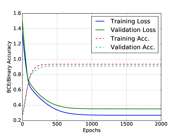
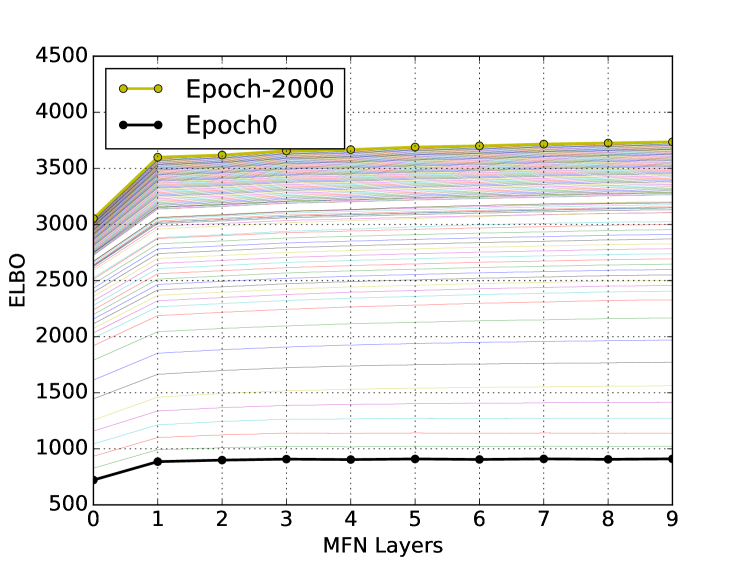
Figure 1: Training and validation losses for MFN along with the binary accuracies averaged over the four-folds of the cross-validation procedure are shown in the figure to left. Binary accuracy is obtained by thresholding predicted probability, i.e., ${\mathbf{S}}^{(t)}={\mathbb{I}}[{\boldsymbol{\alpha}}^{(t)}>0.5]$. Figure to the right shows the ELBO computed at each layer within an epoch and across epochs averaged over four folds.

3.0.3 Learning of Parameters

We create sub-images comprising of $500$ nodes (batch) from each image and derive the corresponding adjacency matrices to reduce memory footprint during the training procedure. Parameters of the MFN are learned by minimizing the BCE loss in (8) computed using all batches of all images in the training data using back-propagation with Adam optimiser with recommended settings [8]. To further reduce computational overhead we restrict the neighbourhood of each node to be $L=10$ nearest neighbours based on Euclidean distance of their locations in the image data. Based on initial investigations of ELBO we set the number of layers in MFN, $T=10$. The learning curves for loss and binary accuracy are shown in Figure 1, along with the ELBO plot showing the successive increase in ELBO with each iteration within an epoch (as guaranteed by MFA) and with increasing epochs (due to gradient descent).

Table 1: Performance comparison based on 4-fold cross validation.

Method	$d_{FP}$(mm)	$d_{FN}$(mm)	$d_{err}$ (mm)
Voxel Classifier	$0.792$	$4.807$	$2.799\pm 0.701$
Bayesian Smoothing	$0.839$	$2.812$	$1.825\pm 0.232$
MFN	$0.835$	$2.571$	$1.703\pm 0.186$

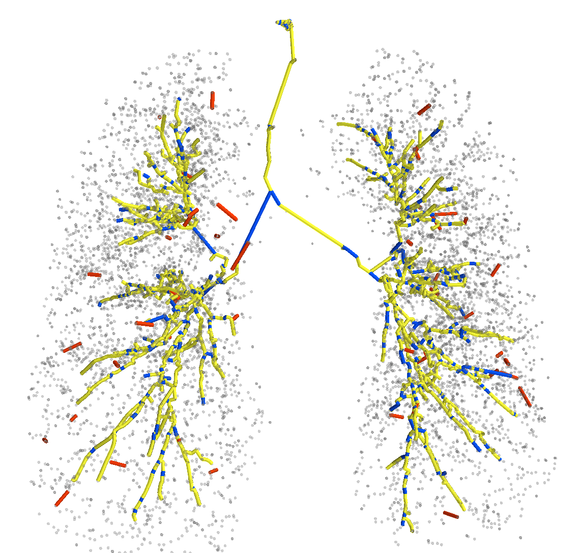
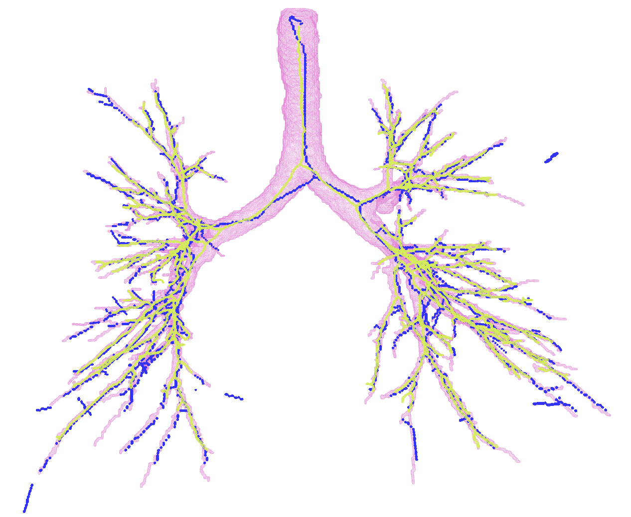
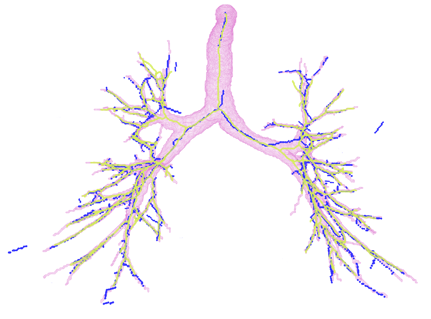
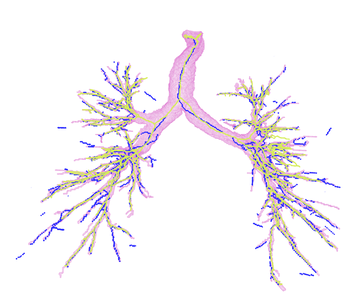
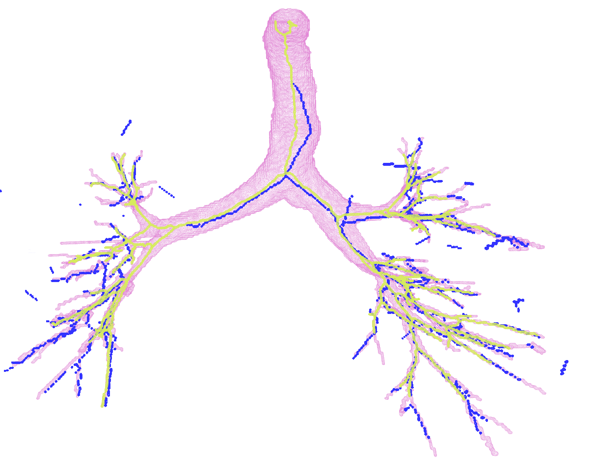
Figure 2: Figure on left: Predicted connections by MFN for one case: Yellow edges are true positives, red edges are false positives and blue are false negatives. Figure on right: Airway tree centerlines for four cases obtained from MFN predictions (blue) overlaid with the reference segmentations (pink surface) and the centerlines from the voxel-classifier based region growing method (yellow).

3.0.4 Results

We compare performance of the proposed MFN method with a method close to the voxel classifier approach that uses region growing on probability images  [6] which was one of the best performing methods in the EXACT’09 challenge [7], and Bayesian smoothing method used in tandem with the voxel classifier approach [11]. We perform 4-fold cross validation using the 32 images on all three methods and report centerline distance based performance measure, $d_{err}$ in mm, in Table 1 based on the cross validation predictions. Our method shows an improvement in the average error with significant gains $(p<0.05)$ by reducing the false negative error $d_{FN}$, implying extraction of more complete trees, when compared to both methods. The results were compared based on paired-sample $t$-test.

In Figure 2, first we present the predicted subgraph for one of the images. The gray dots are nodes of the over-complete graph with features, ${\mathbf{x}}_{i}$, extracted using Bayesian smoothing; the edges are colour-coded providing an insight into the performance of the method: yellow edges are true positives, red edges are false positives and blue edges are false negatives compared to the ground truth connectivity derived from the reference segmentations. Several of the false negatives are spaced closely, and in fact, do not contribute to the false negative error, $d_{FN}$, after generating the binary segmentations. The figure to the right in Figure 2 shows four predicted centerlines overlaid with the reference segmentation and centerlines from the voxel-classifier approach. Clearly, the MFN method is able to detect more branches as seen in most of the branch ends, which is also captured as the reduction in $d_{FN}$ in Table 1. Some of the false positive predictions from MFN method appear to be a missing branch in the reference as seen in the first of the four scans. However, there are few other false positive predictions that could be due to the model using only pairwise potentials; this can be alleviated either by using higher order neighbourhood information or with basic post-processing. The centerlines extracted from MFN are slightly offset from the center of airways at larger scales; this could be due to the sparsity of the nodes at those scales and can be overcome by increasing resolution of the input graph.

4 Discussion and Conclusion

We presented a novel method to perform tree extraction by posing it as a graph refinement task in a probabilistic graphical model setting. We performed approximate probabilistic inference on this model, to obtain a subgraph representing airway-like structures from an over-complete graph, using mean field approximation. Further, using mean field networks we showed the possibility of learning parameters of the underlying graphical model from training data using back-propagation algorithm. The main contribution within the presented MFN framework is our formulation of unary and pairwise potentials as presented in (2) and (3). By designing these potentials to reflect the nature of tasks we are interested in, the model can be applied to a diverse set of applications. We have shown its application to extract airway trees with significant improvement in the error measure, when compared to the two comparison methods. However, tasks like tree extraction can benefit from using higher order potentials that take more than two nodes jointly into account. This limitation is revealed in Figure 2, where the resulting subgraph from MFN is not a single, connected tree. While we used a linear data term in the node potential, ${\mathbf{a}}^{T}{\mathbf{x}}_{i}$ in (2), and a polynomial kernel of degree 1 in the pairwise potential to learn features from data, $\boldsymbol{\nu}^{T}({\mathbf{x}}_{i}{\mathbf{x}}_{j})$ in (3), there are possibilities of using more complex data terms to learn more expressive features, like using a Gaussian kernel as in [10]. Another interesting direction could be to use a smaller neural network to learn pairwise or higher-order features from the node features. On a GNU/Linux based standard computer with 32 GB of memory running one full cross validation procedure on 32 images upto 6 hours. Predictions using a trained MFN takes less than a minute per image.

Our model can be seen as an intermediate between an entirely model-based solution and an end-to-end learning approach. It can be interpreted as a structured neural network where the interactions between layers are based on the underlying graphical model, while the parameters of the model are learned from data. This, we believe, presents an interesting link between probabilistic graphical models and neural network-based learning.

Acknowledgements

This work was funded by the Independent Research Fund Denmark (DFF) and Netherlands Organisation for Scientific Research (NWO).

5 Appendix

We provide the proof for obtaining the mean field approximation update equations in (6) and (7) starting from the variational free energy in equation (4). We start by repeating the expression for the node and pairwise potentials.

Node potential:

$$\phi_{i}({\mathbf{s}}_{i})=\sum_{v=0}^{2}\beta_{v}{\mathbb{I}}\Big{[}\sum_{j}s_{ij}=v\Big{]}+{\mathbf{a}}^{T}{\mathbf{x}}_{i}\sum_{j}s_{ij},$$ (9)

Pairwise potential:

$$\phi_{ij}({\mathbf{s}}_{i},{\mathbf{s}}_{j})=\lambda\big{(}1-2|s_{ij}-s_{ji}|\big{)}+(2s_{ij}s_{ji}-1)\Big{[}\boldsymbol{\eta}^{T}|{\mathbf{x}}_{i}-{\mathbf{x}}_{j}|+\boldsymbol{\nu}^{T}({\mathbf{x}}_{i}{\mathbf{x}}_{j})\Big{]}.$$ (10)

The variational free energy is given as,

$${\mathcal{F}}(q_{\mathbf{S}})=\ln Z+{\mathbb{E}}_{q_{{\mathbf{S}}}}\Big{[}\ln p({\mathbf{S}}|{\mathbf{X}})-\ln q({\mathbf{S}})\Big{]}.$$ (11)

Plugging in (9) and (10) in (11), we obtain the following:

$${\mathcal{F}}(q_{\mathbf{S}}) =\ln Z+{\mathbb{E}}_{q_{{\mathbf{S}}}}\Big{[}\sum_{i\in{\mathcal{N}}}\Big{\{}\beta_{0}{\mathbb{I}}\big{[}\sum_{j}s_{ij}=0\big{]}+\beta_{1}{\mathbb{I}}\big{[}\sum_{j}s_{ij}=1\big{]}+\beta_{2}{\mathbb{I}}\big{[}\sum_{j}s_{ij}=2\big{]}+{\mathbf{a}}^{T}{\mathbf{x}}_{i}\sum_{j}s_{ij}\Big{\}}$$

$$+\sum_{(i,j)\in{\mathcal{E}}}\Big{\{}\lambda\big{(}1-2|s_{ij}-s_{ji}|\big{)}+(2s_{ij}s_{ji}-1)\Big{[}\boldsymbol{\eta}^{T}|{\mathbf{x}}_{i}-{\mathbf{x}}_{j}|+\boldsymbol{\nu}^{T}({\mathbf{x}}_{i}{\mathbf{x}}_{j})\Big{]}\Big{\}}-\ln q({\mathbf{S}})\Big{]}.$$ (12)

We next take expectation ${\mathbb{E}}_{q_{{\mathbf{S}}}}$ using the mean-field factorisation that $q({\mathbf{S}})=\prod_{i=1}^{N}\prod_{j\in{\mathcal{N}}_{i}}q_{ij}(s_{ij})$ and the fact that $\Pr\{s_{ij}=1\}=\alpha_{ij}$ we simplify each of the factors :

$${\mathbb{E}}_{q_{{\mathbf{S}}}}\Big{[}\beta_{0}{\mathbb{I}}\big{[}\sum_{j}s_{ij}=0\big{]}\Big{]}={\mathbb{E}}_{q_{{i1}}\dots q_{{iN}}}\beta_{0}{\mathbb{I}}\big{[}\sum_{j}s_{ij}=0\big{]}\Big{]}=\beta_{0}\prod_{j\in{\mathcal{N}}_{i}}(1-\alpha_{ij}).$$ (13)

Similarly,

$${\mathbb{E}}_{q_{{\mathbf{S}}}}\Big{[}\beta_{1}{\mathbb{I}}\big{[}\sum_{j}s_{ij}=1\big{]}\Big{]}=\beta_{1}\prod_{j\in{\mathcal{N}}_{i}}(1-\alpha_{ij})\sum_{j\in{\mathcal{N}}_{i}}\frac{\alpha_{im}}{(1-\alpha_{im})}$$ (14)

and

$${\mathbb{E}}_{q_{{\mathbf{S}}}}\Big{[}\beta_{2}{\mathbb{I}}\big{[}\sum_{j}s_{ij}=2\big{]}\Big{]}=\beta_{2}\prod_{j\in{\mathcal{N}}_{i}}(1-\alpha_{ij})\sum_{m\in{\mathcal{N}}_{i}}\sum_{n\in{\mathcal{N}}_{i}\backslash m}\frac{\alpha_{im}}{(1-\alpha_{im})}\frac{\alpha_{in}}{(1-\alpha_{in})}.$$ (15)

Next, we focus on the pairwise symmetry term:

$${\mathbb{E}}_{q_{{\mathbf{S}}}}\Big{[}\lambda\big{(}1-2|s_{ij}-s_{ji}|\big{)}\Big{]}=\lambda\big{(}1-2(\alpha_{ij}+\alpha_{ji})+4\alpha_{ij}\alpha_{ji}\big{)}$$ (16)

Using these simplified terms, and taking the expectation over the remaining terms, we obtain the ELBO as,

$${\mathcal{F}}{q_{{\mathbf{S}}}}=\ln Z+\sum_{i\in{\mathcal{N}}}\prod_{j\in{\mathcal{N}}_{i}}(1-\alpha_{ij})\Big{\{}\beta_{0}+\sum_{m\in{\mathcal{N}}_{i}}\frac{\alpha_{im}}{(1-\alpha_{im})}\Big{[}\beta_{1}+\beta_{2}\sum_{n\in{\mathcal{N}}_{i}\setminus m}\frac{\alpha_{in}}{(1-\alpha_{in})}\Big{]}$$

$$+{\mathbf{a}}^{T}{\mathbf{x}}_{i}\sum_{j}\alpha_{ij}\Big{\}}+\sum_{i\in{\mathcal{N}}}\sum_{j\in{\mathcal{N}}_{i}}\Big{\{}\lambda\big{(}1-2(\alpha_{ij}+\alpha_{ji})+4\alpha_{ij}\alpha_{ji}\big{)}-\Big{(}\alpha_{ij}\ln{\alpha_{ij}}$$

$$+(1-\alpha_{ij})\ln(1-{\alpha_{ij}})\Big{)}+(2\alpha_{ij}\alpha_{ji}-1)\Big{[}\boldsymbol{\eta}^{T}|{\mathbf{x}}_{i}-{\mathbf{x}}_{j}|+\boldsymbol{\nu}^{T}({\mathbf{x}}_{i}{\mathbf{x}}_{j})\Big{]}\Big{\}}.$$ (17)

We next differentiate ELBO in (17) wrt $\alpha_{kl}$ and set it to zero.

$$\frac{\partial{\mathcal{F}}{q_{{\mathbf{S}}}}}{\partial\alpha_{kl}} =-\Big{[}\ln\frac{\alpha_{kl}}{1-\alpha_{kl}}\Big{]}+\prod_{j\in{\mathcal{N}}_{k}\setminus l}\big{(}1-\alpha_{kj}\big{)}\Big{\{}\sum_{m\in{\mathcal{N}}_{k}\setminus l}\frac{\alpha_{km}}{(1-\alpha_{km})}\Big{[}(\beta_{2}-\beta_{1})-\beta_{2}\sum_{n\in{\mathcal{N}}_{k}\setminus l,m}\frac{\alpha_{kn}}{(1-\alpha_{kn})}\Big{]}$$

$$+\big{(}\beta_{1}-\beta_{0}\big{)}\Big{\}}+{\mathbf{a}}^{T}{\mathbf{x}}_{i}+(4\alpha_{lk}-2)\lambda+2\alpha_{lk}\big{(}\boldsymbol{\eta}^{T}|{\mathbf{x}}_{i}-{\mathbf{x}}_{j}|+\boldsymbol{\nu}^{T}({\mathbf{x}}_{i}{\mathbf{x}}_{j})\big{)}.\qquad=0$$ (18)

From this we obtain the MFA update equation for iteration $(t+1)$ based on the states from $(t)$,

$$\alpha_{kl}^{(t+1)}=\sigma({\gamma_{kl}})=\frac{1}{1+\exp^{-\gamma_{kl}}}\text{ }\forall\text{ }{k}=\{1\dots N\},\text{ }l\in{\mathcal{N}}_{k}\text{ }:\text{ }|{\mathcal{N}}_{k}|=L$$ (19)

where $\sigma(.)$ is the sigmoid activation function, ${\mathcal{N}}_{k}$ are the $L$ nearest neighbours of node $k$ based of positional Euclidean distance, and

$$\gamma_{kl}=\prod_{j\in{\mathcal{N}}_{k}\setminus l}\big{(}1-\alpha_{kj}^{(t)}\big{)}\Big{\{}\sum_{m\in{\mathcal{N}}_{k}\setminus l}\frac{\alpha_{km}^{(t)}}{(1-\alpha_{km}^{(t)})}\Big{[}(\beta_{2}-\beta_{1})-\beta_{2}\sum_{n\in{\mathcal{N}}_{k}\setminus l,m}\frac{\alpha_{kn}^{(t)}}{(1-\alpha_{kn}^{(t)})}\Big{]}$$

$$+\big{(}\beta_{1}-\beta_{0}\big{)}\Big{\}}+{\mathbf{a}}^{T}{\mathbf{x}}_{i}+(4\alpha_{lk}^{(t)}-2)\lambda+2\alpha_{lk}^{(t)}\big{(}\boldsymbol{\eta}^{T}|{\mathbf{x}}_{i}-{\mathbf{x}}_{j}|+\boldsymbol{\nu}^{T}({\mathbf{x}}_{i}{\mathbf{x}}_{j})\big{)}.$$ (20)

References

- [1] Jaakkola, Tommi S., Michael I. Jordan. ”Improving the mean field approximation via the use of mixture distributions.” Learning in graphical models. Springer(1998)
- [2] Zhang, Yongyue, Michael Brady, and Stephen Smith. ”Segmentation of brain MR images through a hidden Markov random field model and the expectation-maximization algorithm.” IEEE transactions on medical imaging 20.1 (2001): 45-57.
- [3] Wang, XiaoFeng, and Xiao-Ping Zhang. ”A new localized superpixel Markov random field for image segmentation.” Multimedia and Expo, 2009. ICME 2009. IEEE International Conference on. IEEE, 2009
- [4] Lo, Pechin, et al. ”Airway tree extraction with locally optimal paths.” International Conference on Medical Image Computing and Computer-Assisted Intervention. Springer, Berlin, Heidelberg, 2009.
- [5] Pedersen, Jesper H., et al. ”The Danish randomized lung cancer CT screening trial—overall design and results of the prevalence round.” Journal of Thoracic Oncology 4.5 (2009): 608-614.
- [6] Lo, Pechin, et al. ”Vessel-guided airway tree segmentation: A voxel classification approach.” Medical image analysis 14.4 (2010): 527-538.
- [7] Lo, Pechin, et al. ”Extraction of airways from CT (EXACT’09).” IEEE Transactions on Medical Imaging 31.11 (2012): 2093-2107.
- [8] Kingma, Diederik P., and Jimmy Ba. ”Adam: A method for stochastic optimization.” arXiv preprint arXiv:1412.6980 (2014).
- [9] Li, Yujia, and Richard Zemel. ”Mean-Field Networks.” arXiv preprint arXiv:1410.5884 (2014).
- [10] Orlando, José Ignacio, and Matthew Blaschko. ”Learning fully-connected CRFs for blood vessel segmentation in retinal images.” International Conference on Medical Image Computing and Computer-Assisted Intervention. Springer, Cham, 2014.
- [11] Selvan, Raghavendra, et al. ”Extraction of Airways with Probabilistic State-space Models and Bayesian Smoothing.” Graphs in Biomedical Image Analysis, Computational Anatomy and Imaging Genetics. Springer, Cham, 2017. 53-63.