The KMTNet 2016 Data Release

Abstract

We present Korea Microlensing Telescope Network (KMTNet) light curves for microlensing-event candidates for the 2016 season, which covers an area of $97\,\deg^{2}$ observed at cadences ranging from $\Gamma=0.2\,{\rm hr}^{-1}$ to $\Gamma=8\,{\rm hr}^{-1}$ from three southern sites in Chile, South Africa, and Australia. These 2163 light curves are comprised of 1856 “clear microlensing” and 307 “possible microlensing” events (including 265 previously released from the K2 C9 field). The data policy is very similar to the one governing the 2015 release. The changes relative to 2015 in the algorithms to find and vet microlensing events are comprehensively described.

1 Introduction

A major goal of the Korea Microlensing Telescope Network (KMTNet, Kim et al. 2016) is to provide timely public access to all of the microlensing light curves found by the KMTNet team, including both “clear” and “possible” events (Kim et al., 2018a). These events are found by applying the “event finder” algorithm described by Kim et al. (2018a) to roughly $3\times 10^{8}$ light curves that are derived from data taken by three identical $4\,\deg^{2}$ cameras mounted on three identical 1.6m telescopes located in Chile (KMTC), South Africa (KMTS), and Australia (KMTA).

The first such data release was for the 2015 commissioning-year data set (Kim et al., 2018a). While the basic goals and data release policy are very similar to that work, there are many concrete differences reflected in the 2016 release. The data set itself is substantially different (Section 2), the event-finder algorithm has been upgraded, including additional checks for false positives (Section 3), and the data products have been substantially upgraded as well (Section 4). The data policy is also slightly altered for 2016 in that a subset of the data (Kim et al., 2018b) was released in an expedited fashion. We briefly review these data policies (as slightly modified) in Section 5.

2 2016 Data

The 2016 KMTNet data differ in two major respects compared to 2015. First, we observed a total of 27 fields covering $97\,\deg^{2}$ in 2016 compared to four fields covering $16\,\deg^{2}$ in 2015. Second, in 2016, the data from all three sites were reduced and jointly fit to microlensing light-curve profiles to find candidate events. By contrast, in 2015, only KMTC data were initially fit to microlensing profiles, and the data from KMTS and KMTA were only reduced for candidates that were identified based on KMTC data.

The layout and nominal cadence of the 27 fields observed in 2016 is shown in Figure 12 of Kim et al. (2018a). Conceptually, there are three “prime fields” covering $12\,\deg^{2}$ that are observed at a cadence of $\Gamma=4\,{\rm hr}^{-1}$. In practice, each of these is observed in pairs (BLG01/BLG41, BLG02/BLG42, BLG03/BLG43) that are offset by about $8.4^{\prime}$ (in order to cover the gaps between the four chips in each field), all with a nominal per field cadence of $\Gamma=2\,{\rm hr}^{-1}$. Moreover, two of these pairs of fields (BLG02/BLG42 and BLG03/BLG43) overlap by about $0.4\,\deg^{2}$. Finally, about $0.35\,\deg^{2}$ of the “offset fields” BLG41 and BLG43 that do not overlap other prime fields, do overlap the $\Gamma=1\,{\rm hr}^{-1}$ fields (see below) BLG04 and BLG22. Hence the “prime fields” actually comprise a total of about $13.1\,\deg^{2}$ consisting of $0.4\,\deg^{2}$ with $\Gamma=8\,{\rm hr}^{-1}$, $9.7\,\deg^{2}$ with $\Gamma=4\,{\rm hr}^{-1}$, $0.35\,\deg^{2}$ with $\Gamma=3\,{\rm hr}^{-1}$, and $2.65\,\deg^{2}$ with $\Gamma=2\,{\rm hr}^{-1}$.

The remaining 21 fields covering $84\,\deg^{2}$ (less the $0.35\,\deg^{2}$ just mentioned) are divided into three groups: 7 fields with cadence $\Gamma=1\,{\rm hr}^{-1}$ (BLG04, BLG14, BLG15, BLG17, BLG18, BLG19, and BLG22), 11 fields with cadence $\Gamma=0.4\,{\rm hr}^{-1}$ (BLG11, BLG16, BLG20, BLG21, BLG31, BLG32, BLG33, BLG34, BLG35, and BLG38), and 3 fields with cadence $\Gamma=0.2\,{\rm hr}^{-1}$ (BLG12, BLG13, and BLG36). Figure 1 shows the density of catalog stars in these fields (but excluding BLG41, BLG42, and BLG43, to avoid clutter).

This nominal cadence was followed by KMTC for all of 2016, and it was followed for most of 2016 by KMTS and KMTA. However, this cadence structure was adjusted to support the Kepler K2C9 campaign (Gould & Horne, 2013; Henderson et al., 2016; Kim et al., 2018b) from April 23 to June 16. During this period (for KMTS and KMTA), the cadences of fields BLG02, BLG42, BLG03, and BLG43 were increased by a factor 1.5 from $\Gamma=2\,{\rm hr}^{-1}$ to $\Gamma=3\,{\rm hr}^{-1}$, while those of all other fields were decreased by a factor 0.75. That is, the cadences were $\Gamma=1.5\,{\rm hr}^{-1}$ (2 fields), $\Gamma=0.75\,{\rm hr}^{-1}$ (7 fields), $\Gamma=0.3\,{\rm hr}^{-1}$ (11 fields), and $\Gamma=0.15\,{\rm hr}^{-1}$ (3 fields).

Finally, we note that in 2016, 10/11 of observations at KMTC, 20/21 of observations at KMTS, and all observations at KMTA were taken $I$ band. The remaining observations (roughly 5% of the total) were taken in $V$ band.

3 2016 Event Finder

The major modifications to the Event Finder algorithm (originally described in Kim et al. 2018a) for 2016 are detailed below. The major change to the algorithm itself was to combine light curves from multiple sites and multiple fields (Section 3.1). Another major change was to remove known variables either from published catalogs or previous years’ work (Section 3.2). We also augmented our automated candidate vetting by writing two new algorithms whose purposes were to reject “short-timescale artifacts” (Section 3.3) and “periodic variables” (Section 3.4), respectively. Because the Event Finder algorithm was continually developed, these algorithms were only applied to the data analyzed after their development, i.e., they were incorporated starting approximately at the point just after the prime fields were completed. Section 3.5 describes the final vetting procedures and summarizes the discoveries.

3.1 Combined Light Curves

The event finder was changed in 2016 in a number of important respects. The most important change is that we searched for events in all three data sets simultaneously. As discussed by Kim et al. (2018a), light curves were constructed at the locations of input-catalog stars using the difference imaging analysis (DIA) code of Woźniak (2000). Because the input catalog is identical for all three observatories, it is straightforward to cross-identify the light curves. (This was not possible in 2015 because there was insufficient computing power to reduce data from all three sites in a timely way. Moreover, the commissioning character of the data would have made combined analysis quite difficult in any case.)

A second major change was that we combined the analysis of light curves from overlapping fields. For example, in the overlap regions between BLG02/BLG42/BLG03/BLG43, a total of 12 light curves were jointly analyzed, i.e., (3 observatories)$\times$(4 fields). This was unnecessary in 2015 because there were no overlapping fields.

However, we only combined overlapping fields for catalog stars derived from the OGLE-III catalog (Szymański et al., 2011). Only these catalog entries could be unambiguously cross-identified between overlapping fields. For areas that are not covered by OGLE-III, the star catalog was derived using DoPhot (Schechter et al., 1993) on each field separately. Although fields BLG01, BLG02, and BLG03 were moved slightly between 2015 and 2016, one can gain a good impression of the location of these non-OGLE-III areas from Figure 8 of Kim et al. (2018a). See also Figure 1 of this paper.

3.2 Removing Known Variables and Artifacts

Another important change was the removal of published variables prior to the stage of showing the light curves of candidates to the operator. Recall from Kim et al. (2018a) that after individual candidates are cataloged, they are grouped using a friends-of-friends algorithm, so that only the “best” (in terms of $\Delta\chi^{2}$) is shown to the operator. However, if this “group leader” is in a published catalog of variables, then the entire group is skipped. For this purpose, we used the OGLE-long-period-variable (Soszyński et al., 2013) and OGLE-dwarf-nova (Mróz et al., 2015) catalogs.

Similarly, if the “group leader” is identified as an earlier-year candidate that was flagged as a variable or as an artifact, it is also not shown. Of course, for 2016 “earlier year” can only refer to 2015 and so only to stars in BLG01, BLG02, BLG03, and BLG04 from that year. Moreover, because these fields all moved slightly, we could only apply this procedure to OGLE-III catalog stars, but in any case these are the overwhelming majority in these fields. In fact, in 2016, we only matched the 2016 “group leaders” to the list of 2015 “group leaders” of variables and artifacts. A more robust approach would be to match to all the 2015 stars that were in these variable and artifact groups, not just the “leaders”. Unfortunately we only realized this when we had completed the review of the fields that overlapped the 2015 fields. However, the more robust approach will be implemented in 2017 and future years.

Finally, we also matched to all previous-year OGLE and MOA events, as listed on their web pages. For 2016, these identifications were made after the event selection, i.e., at the same time as the selected candidates were cross-identified with current year (2016) OGLE and MOA events. However, for 2017 and future years, earlier-year OGLE and MOA events will be flagged to the operator’s attention at the time that the candidate is reviewed. Almost all such matches in 2016 were to OGLE, and the great majority of these were to candidates from more than two years previously. While we did consider the possibility that these were repeating microlensing events, in all cases we concluded that they were cataclysmic variables (CVs) or other outbursting variables, which happened to look something like microlensing events in their earliest appearance in OGLE data and also in the 2016 KMT data. A number of matches were long timescale events for which OGLE issued an alert in 2015.

3.3 Short-Timescale Artifacts

The great majority of short-timescale artifacts consist of 1–2 isolated spurious points, usually in a single night, that are then almost perfectly fit to a microlensing profile (which has two continuous free parameters). These can occasionally be “coordinated” between observatories, in particular if they are caused by the Moon passing through the bulge. Because the fit is “perfect”, the $\chi^{2}$ renormalization process described by Kim et al. (2018a) automatically generates a very high $\Delta\chi^{2}$. We search for these artifacts by finding the two data points from each observatory/field combination that contribute the most to $\Delta\chi^{2}$ and then removing their contribution. If the event fails the $\Delta\chi^{2}$ criterion after this removal, it is eliminated. This algorithm was applied to the grouped-candidate list for the outlying fields in 2016 but not for the prime fields, BLG01/02/03/41/42/43, because it was developed after visual inspection of these fields. However, for 2017 and future years, it will be included directly in the event-finder pipeline.

Prior to implementing the “short-timescale artifact” finder described above, we employed a somewhat less precise method of removing such short-timescale artifacts. For each field, and for each of the four chips, we counted the number of candidates with a given $(t_{0},t_{\rm eff})$. If one of these bins contained more than 1% of all pairs and had $t_{\rm eff}\leq 2\,$days, we eliminated the entire bin. That is, we took the very high number of candidates in a bin as an indication that they had a common cause in the observing conditions, such as interplay between a bright moon and camera optics. It is possible that a handful of real microlensing events were eliminated in this way, but the method was essential to eliminating several hundred thousand spurious candidates (given that we had not yet invented the “short-timescale artifact” remover).

3.4 Periodic-Variable Finder

The term “periodic variable” conveys two distinct ideas. Normally, one considers that the profile of its “variation” should repeat (or approximately repeat) according to some regular (or nearly regular) “period”. While there is no shortage of such variables, there are also stars that vary quite regularly, but show very different amplitudes of variation (and sometimes forms of variation) at each cycle. We therefore adapted the event finder to identify both types.

Recall that, as originally constructed, the event finder would fit two flux parameters to each of several thousand different magnification profiles that are defined by $(t_{0},t_{\rm eff})$, i.e., the time of peak magnification and the effective timescale. The fits are restricted to data lying within $t_{0}\pm 5\,t_{\rm eff}$. In the event finder itself, only the best fit is kept. The periodic-variable finder instead keeps the top 50 $(t_{0},t_{\rm eff})$ pairs and then restricts consideration to those with $\Delta\chi^{2}>0.2\Delta\chi^{2}_{\rm max}$.

It then attempts to find “periodic behavior” in a subset of the 50 cataloged $(t_{0},t_{\rm eff})$ pairs. This subset is defined as the profiles for which $t_{\rm eff}=t_{{\rm eff},{\rm max}}$, where $t_{{\rm eff},{\rm max}}$ is the effective timescale of the best-fit profile. First, “peaks” (in $t_{0}$) are successively identified within this subset. The first “peak” is simply the $(t_{0},t_{{\rm eff},{\rm max}})$ with the highest $\Delta\chi^{2}$. All pairs $(t_{0},t_{{\rm eff},{\rm max}})$ within $t_{{\rm eff},{\rm max}}$ of this peak are then grouped with it and eliminated from further consideration, and the second “peak” is chosen as the $(t_{0},t_{{\rm eff},{\rm max}})$ with the highest $\Delta\chi^{2}$ among those remaining. This process is repeated until the $(t_{0},t_{{\rm eff},{\rm max}})$ subset is exhausted.

Then, the algorithm checks to see if there are multiple peaks with the same period. Based on a review of real periodic variables (of all types), we restrict consideration to periods $P$ satisfying $5<P/t_{{\rm eff},{\rm max}}<13$. That is, if the peak of a periodic variable is fitted to a microlensing profile, the fit will typically have an effective timescale that is about 12% of the period, with some variation. If there are three or more cataloged $(t_{0},t_{{\rm eff},{\rm max}})$ pairs that are matched within $t_{{\rm eff},{\rm max}}$ of a predicted peak for a given trial period $P$, then we exclude the star as a “periodic variable”. If there are only two $(t_{0},t_{{\rm eff},{\rm max}})$ pairs, then we conduct two additional tests, both of which begin by identifying the “best” period, i.e., the one that produces the closest match to the second peak of $t_{{\rm eff},{\rm max}}$ profiles.

First, we check whether there are other $t_{\rm eff}$ (i.e., other than $t_{{\rm eff},{\rm max}}$) for which there are three or more peaks that line up with the “best” period derived from the $(t_{0},t_{{\rm eff},{\rm max}})$ profiles. If so, we eliminate the star. If not, then we ask whether $(P,t_{{\rm eff},{\rm max}})$ satisfy two further conditions. The first condition is that $P$ lies in the restricted range $6<P/t_{{\rm eff},{\rm max}}<10$, which is populated by a substantial majority of real variables. Second, we demand $P>T/4$, where $T$ is the duration of the season. This guarantees first that the interval between peaks is quite long, i.e., $\gtrsim 60\,$days, and second that no more than one peak from the periodic variable is “missed” (due to low amplitude).

Elimination of such two-peak “periodic” variables may seem dangerous at first sight because any two peaks would seem to satisfy the criteria. Recall, however, that the range of periods is quite restricted. While it is not difficult to construct a wide-binary microlensing event that satisfies these criteria, the fraction of random events that actually do satisfy them is quite small. The second component of the binary must yield a fit with the same $t_{\rm eff}$ as the first with $\geq 20\%$ of its $\Delta\chi^{2}$, and the separation between peaks must be in a narrow range determined by this $t_{\rm eff}$. Moreover, the inferred period must be at least $P\gtrsim 60\,$days. This mode of rejection is quite effective at rejecting long-period variables. It does induce a small amount of risk, and for this reason it may be eliminated in some future year when the great majority of such long-period variables are already cataloged.

3.5 Final Vetting

After all “clear” and “possible” microlensing events were selected, we performed two additional inspections. First, we had developed a special pipeline to generate high-quality pySIS (Albrow et al., 2009) reductions, which was mainly for the purpose of the data release (see Section 4). However, inspection of these higher-quality reductions was also useful to identify variables of various kinds, particularly CVs.

Second, we examined the combined 2016-2017 DIA light curves. It was not our original intention to do this because it obviously required waiting until most or all of the 2017 season was over. However, by the time the pySIS pipeline was debugged and implemented, all 2017 DIA reductions were complete. In fact, these combined light curves proved quite valuable in identifying long-period variables as well as repeating variables, probably mostly CVs. Indeed, because quite a few of these “repeaters” had only one other outburst within the two years (actually, two seasons) of data, it is very likely that there are other “repeaters” masquerading as microlensing events, whose frequency of repetition is yet lower.

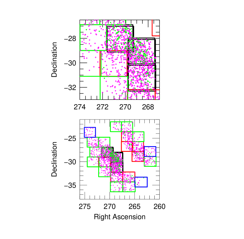
Figure 2: Distribution in equatorial coordinates of the 2163 microlensing events found by KMTNet from its 2016 data, including 1856 “clear” (magenta) and 307 “possible” (green) events. The KMT fields are outlined and color-coded by cadence, with (black, red, green, blue) corresponding to $\Gamma=(2,1,0.4,0.2)\,{\rm hr}^{-1}$. See Figure 12 from Kim et al. (2018a) for the field-numbering scheme. The upper panel highlights the 6 overlapping high-cadence fields (clockwise from upper left), BLG03/43, BLG02/42, BLG01/41 .

In all, the event finder found 3,045,815 candidates, which the friends-of-friends algorithm grouped into 1,123,819 groups. 102,121 of these were eliminated as variables by matching to published catalogs or to 2015 KMTNet variables or by the periodic-variable finder. 601,174 were eliminated by matching to previous artifacts or by one of the two variants of artifact finder discussed above. This left 420,524 candidates to be viewed by operator. Among these, 2065 were chosen as “clear microlensing” and 532 as “possible microlensing”. Of these 134 proved to be duplicates. Then based on inspection of their 2016 pySIS light curves and their 2016-2017 DIA light curves, a further 300 candidates were eliminated, leaving 1856 “clear microlensing” and 307 “possible microlensing” events. A map of these events is shown in Figure 2.

4 Data Products

All the data for this release are available at http://kmtnet.kasi.re.kr/ulens/ from which one can access http://kmtnet.kasi.re.kr/ulens/event/2016/ .

For almost all events, one can access DIA and pySIS data in two forms, pictorial and ascii data files. In a few cases the automated pySIS reductions failed. The page of each event contains a finding chart and the best fit $(t_{0},t_{\rm eff},u_{0})$ parameters from the original search as well as cross-identification to OGLE and/or MOA listings.

5 Data Policy

Our data policy is basically the same as for 2015 (which we also anticipate will be the long term policy), and we urge the reader interested in using the data presented here to read that policy in Kim et al. (2018a). Here we re-emphasize only the most essential points and describe the small deviations from the 2015 policy.

The central point is that all data presented in Section 4 will become free for public use as soon as this paper and all papers that use these data and that have already been submitted are accepted for publication. Prior to that time, papers can be prepared for publication using these data, but they cannot be submitted to journals nor posted on arXiv.

We welcome users of these data to collaborate with the KMTNet team, but we do not insist on it. In particular, while the pySIS pipeline reductions are generally of very high quality, they can in some cases be improved using a tender-loving-care (TLC) approach. Such TLC light curves could be one form of collaboration. However, if other workers would like to do their own re-reductions without our cooperation, we will send postage-stamps of all epochs, provided that we are given solid evidence of advanced preparation of a publishable paper. If requested, such postage stamps would also include $V$-band data.

The 13 submitted papers based on these data are Hwang et al. (2018), Shin et al. (2017, 2018), Mróz et al. (2017), Han et al. (2017b, a), Ryu et al. (2017, 2018), Jung et al. (2017a, b), Calchi Novati et al. (2016), Shvartzvald et al. (2017), and Albrow et al. (2018).

Finally, we note that a subset of the 2016 data release is available without restriction, namely the events that broadly overlap the Kepler K2C9 campaign. As discussed by Kim et al. (2018b), these are available at http://kmtnet.kasi.re.kr/ulens/event/2016k2/ . These same light curves are also available at http://kmtnet.kasi.re.kr/ulens/event/2016/ in order to maintain an integrated record of 2016 KMTNet events. However, we continue to maintain the K2C9 page so there is an unambiguous record of which events have unrestricted access.

6 Future Plans

For 2015 data, we released DIA-pipeline light curves roughly 16 months after the close of the 2015 season. We also set two goals for improvement: first, release high-quality pySIS light curves; second, reduce the delay of release to roughly 6 months after the close of each microlensing season, i.e., roughly April of the following year.

With this release, we have met the first goal but have fallen further behind on the second, i.e., to 18 months after the close of the 2016 season. Nevertheless, on the basis of ongoing practical experience, we believe that the original goal will be achieved for the 2018 release. In particular, the 2017 event selection was completed in early January 2018. However, we could not begin high-quality reductions until April 2018 due to a backlog of work on 2016 data, at which point most computing power was already engaged in the processing of 2018 data. All such backlogs should be cleared by the time 2018 event selection is complete.

Finally, subsequent to the analysis reported here, we have upgraded our star catalog by replacing our own DoPhot-based catalog with the CFHT-based catalog of Schlafly et al. (2018) in all regions that the two coincide. This has increased the overall size of the catalog from $3\times 10^{8}$ to $5\times 10^{8}$ stars. See Figure 1. The new catalog is already being incorporated into the photometry of 2018 KMTNet data. If resources permit, we will reprocess the 2016 and 2017 data using this new catalog as well. In this case, we will update the 2016 webpage with additional events.

Figure 1: Star catalog for 24 of the 27 KMTNet fields showing 1/2000 entries. Fields BLG41/42/43, which strongly overlap BLG01/02/03, are not shown to avoid clutter, but these fill in the chip gaps of the latter three fields. Left: Catalog actually used in 2016. The regions covered by the OGLE-III catalog (Szymański et al., 2011) are substantially denser than those that are not and for which we constructed our own catalog using DoPhot (Schechter et al., 1993). The boundaries between these are sharp and rectilinear. In addition, particularly near the Galactic plane, there are regions of very low star-catalog density due to high extinction. See Figure 12 from Kim et al. (2018a) for the field-numbering scheme. Right: Upgraded catalog that replaces the previous DoPhot catalog with a CFHT catalog (Schlafly et al., 2018), wherever the latter is available. This will be applied to 2018+ data going forward and may be retrospectively applied to 2016 and 2017 data as well.

References

- Albrow et al. (2009) Albrow, M. D., Horne, K., Bramich, D. M., et al. 2009, MNRAS, 397, 2099
- Albrow et al. (2018) Albrow, M.D., Yee, J.C., Udalski, A. et al., 2018, AAS submitted, arXiv:1802.09563
- Calchi Novati et al. (2016) Calchi Novati, S., Suzuki, D., Udalski, A., et al. 2016, AAS submitted, arXiv:1801.05806
- Gould & Horne (2013) Gould, A. & Horne, K. 2013, ApJ, 779, L28
- Han et al. (2017a) Han, C., Udalski, A., Sumi, T. 2017a, ApJ, 843, 59
- Han et al. (2017b) Han, C., Udalski, A., Gould, A. 2017b, AJ, 154, 223
- Henderson et al. (2016) Henderson, C.B., Poleski, R., Penny, M. et al. 2016 PASP128, 124401
- Hwang et al. (2018) Hwang, K.-H., Kim, H.-W., Kim, D.-J., et al. 2018, JKAS, submitted, arXiv:1802.10246
- Jung et al. (2017a) Jung, Y. K., Udalski, A., Yee, J.C., et al. 2017a AJ, 153, 129
- Jung et al. (2017b) Jung, Y. K., Udalski, A., Yee, J.C., et al. 2017b ApJ, 841, 75
- Kim et al. (2018a) Kim, D.-J., Kim, H.-W., Hwang, K.-H., et al., 2018a, AJ, 155, 76
- Kim et al. (2018b) Kim, H.-W.., Hwang, K.-H., Kim, D.-J., et al., 2018b, AJ, in press, arXiv:1801.08166
- Kim et al. (2016) Kim, S.-L., Lee, C.-U., Park, B.-G., et al. 2016, JKAS, 49, 37
- Mróz et al. (2015) Mróz, P., Udalski, A., Poleski, R. et al. 2015, Acta Astron 65, 313
- Mróz et al. (2017) Mróz, P., Han, C., Udalski, A. et al. 2017, AJ, 153, 143
- Ryu et al. (2017) Ryu, Y.H, Udalski, A., Yee, J.C. et al. 2017, AJ, 154, 247
- Ryu et al. (2018) Ryu, Y.H, Yee, J.C., Udalski, A. et al. 2018, AJ, 155, 40
- Schechter et al. (1993) Schechter, P.L., Mateo, M., & Saha, A. 1993, PASP, 105, 1342
- Schlafly et al. (2018) Schlafly, E.F., Green, G.M., Lang, D. et al. 2018, ApJS, 234, 39
- Shin et al. (2017) Shin, I.-G., Udalski, A., Yee, J.C. et al. 2017, AJ, 154, 176
- Shin et al. (2018) Shin, I.-G., Udalski, A., Yee, J.C. et al. 2018, AAS submitted, arXiv:1801.001695
- Shvartzvald et al. (2017) Shvartzvald, Y., Yee, J.C., Calchi Novati, S. et al. 2017, ApJ, 840, L3
- Soszyński et al. (2013) Szymański et al.(2011)]oiiicatSoszyński, I., Udalski, A., Szymański, M.K., et al. 2013, Acta Astron., 63, 21
- Szymański et al. (2011) Szymański, M.K., Udalski, A., Soszyński, I., et al. 2011, Acta Astron., 61, 83
- Woźniak (2000) Woźniak, P. R. 2000, Acta Astron., 50, 421