See Plots/WFIRSTProposalCover_AnnualReport2017.jpg

Cosmology with the WFIRST High Latitude Survey Science Investigation Team
Annual Report 2017

NOTE: The original version of this report was submitted to the WFIRST Project Office on July 14, 2017. Some minor updates have been made in this version.

1 Executive Summary

Cosmic acceleration is the most surprising cosmological discovery in many decades. Even the least exotic explanation of this phenomenon requires an energetically dominant component of the universe with properties never previously seen in nature, pervading otherwise empty space, with an energy density that is many orders of magnitude lower than naive expectations. More broadly, the origin could derive from a novel, dynamically-evolving type of matter or, instead, signal deviations from General Relativity on the large scales and low densities probed by cosmological tracers. Testing and distinguishing among possible explanations requires cosmological measurements of extremely high precision that probe the full history of cosmic expansion and structure growth and, ideally, compare and contrast matter and relativistic tracers of the gravity potential. This program is one of the defining objectives of the Wide-Field Infrared Survey Telescope (WFIRST), as set forth in the New Worlds, New Horizons report (NWNH) Council (2010). The WFIRST mission, as described in the Science Definition Team (SDT) reports (Spergel et al., 2013, 2015, hereafter SDT13 and SDT15 respectively), has the ability to improve these measurements by $1-2$ orders of magnitude compared to the current state of the art, while simultaneously extending their redshift grasp, greatly improving control of systematic effects, and taking a unified approach to multiple probes that provide complementary physical information and cross-checks of cosmological results.

We described in this document the activities of the Science Investigation Team (SIT) Cosmology with the High Latitude Survey. This team was selected by NASA in December 2015 in order to address the stringent challenges of the WFIRST dark energy (DE) program through the Project’s formulation phase. This SIT has elected to address Galaxy Redshift Survey (GRS), Weak Lensing (WL) and Cluster Growth (CL) of the WFIRST Science Investigation Team (SIT) NASA Research Announcement (NRA) with a unified team, because the two investigations are tightly linked at both the technical level and the theoretical modeling level. Our team thus fully embrace the fact that the imaging and spectroscopic elements of the High Latitude Survey (HLS) will be realized as an integrated observing program, and they jointly impose requirements on instrument and telescope performance, operations, and data transfer. We also naturally acknowledge that the methods for simulating and interpreting weak lensing and galaxy clustering observations largely overlap. Many members of our team have expertise in both areas.

WFIRST is designed to be able to deliver a definitive result on the origin of cosmic acceleration. If the growth rate of structure is inconsistent with the evolution of the Hubble constant, this would be the signature of the breakdown of General Relativity on cosmological scales. If the evolution of the Hubble constant is consistent with the growth rate of structure but inconsistent with vacuum energy, then this would imply that dark energy is dynamical. Either result would have a profound impact on our understanding of physics. WFIRST is not optimized for “Figure of Merit” sensitivity but for control of systematic uncertainties in the astronomical measurements and for having multiple techniques each with multiple cross-checks. Our SIT work focuses on understanding the potential systematics in the WFIRST dark energy measurements.

In our proposal, we structured our planning around the series of deliverables described in §2. We will present in this detailed report our progress on these deliverables and illustrate that we either reached or exceeded our proposed expected milestones.

Because the development of the science requirements is at the core of our proposed investigation, we present some broad aspects of our strategy in §3 before giving a summary of the High Latitude Imaging Survey (HLIS) and of the HLS Spectroscopic Survey (HLSS) science requirements as we formulated them to support the WFIRST Project Office in §4 and §5. We present our revised cosmological forecasts and associated trade studies in §6. We also address questions of survey operations and optimization in §7, our actions towards broad community engagement in §8 and discuss in §9 the other ways in which our SIT supported the WFIRST mission.

2 Proposed and Actual Deliverables

In our proposal, we structured our planning around a series of deliverables numbered D1-12. We will use throughout this report the same nomenclature and report on our progress on each of these deliverables when compared to the proposed calendar visible in Figure 1. We will illustrate that we compare favorably on all deliverables. We give in this section a quick summary but will give more details in the relevant sections. We will also explicitly reference the deliverables (D1-12) in the relevant section titles of our report. In the text below, the definition of each deliverables is quoted directly from our proposal and we summarize the progress briefly in italic.

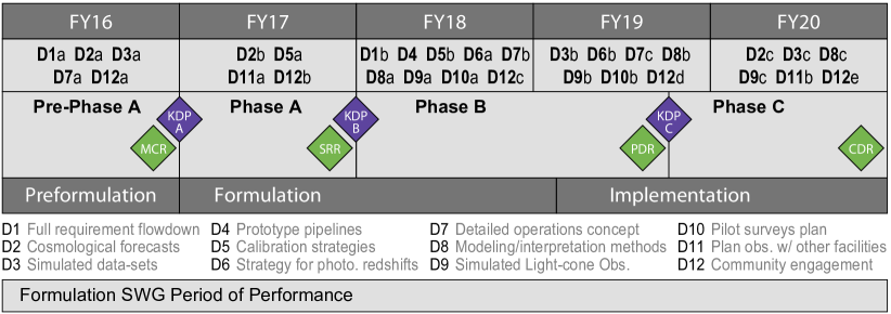
Figure 1: Our proposed deliverable schedule in concordance with the WFIRST project timeline as displayed in the WFIRST SIT call §3.2. Deliverables that are made in multiple stages are labeled (a, b and c) and appear in multiple years. This figure is taken from our original proposal and the schedule has in fact shifted since our investigation started on January 2016, thus well into FY16.

(D1) Full requirements flow-down

from the high-level science goals of the HLS galaxy clustering and weak lensing survey to detailed performance of the telescope, wide field instrument, software, operations, and data transfer. Throughout the year, we delivered three versions of the level 2 science requirements for both the HLSS (§5) and the HLIS (§4).

(D2) Forecasts of the cosmological performance of the HLS Imaging and Spectroscopy data sets,

including expected constraints on dark energy, modified gravity, neutrino masses, and inflation, from analyses that include the measurement of the location of the Baryon Acoustic Oscillations (BAO), Redshift-Space Distortions (RSD), galaxy power spectrum and higher order statistics, cosmic shear, galaxy-galaxy lensing, and cluster demographics. These forecasts incorporate realistic assessments of observational systematics and theoretical modeling systematics, and they examine the expected constraints from different probes individually, in concert with each other, and in concert with expected constraints from the WFIRST supernova program, CMB experiments, and other cosmological surveys such as DESI, LSST, and Euclid. We use our forecasting tools to investigate trades, e.g., the impact of survey or instrument design choices (area, depth, pixel size, spectral resolution, etc.) on cosmological performance. We developed a unique software package (CosmoLike ) that enables us to jointly forecast all the WFIRST cosmological probes, including their covariance (§6). We used this framework to conduct trade studies §6. We released to the community the associated WFIRST chains (§9).

(D3) Simulated imaging and spectroscopic data sets

for testing pipeline performance and evaluating systematic biases — e.g., from confusion, noise, and incompleteness in images and spectra, or errors in Point Spread Function (PSF) determination or shape measurement. These data sets will be created with varying levels of complexity in the source catalogs and instrumental effects, to allow isolation of individual contributions to statistical and systematic uncertainties. Some of these artificial data sets will be made publicly available, and some will take the form of data challenges, where the underlying parameters are initially known only to the creators of the data set, in the spirit of the Shear Testing Program (STEP) and Gravitational Lensing Accuracy Test (GREAT) weak lensing data challenges Heymans et al. (2006); Massey et al. (2007); Bridle et al. (2010); Kitching et al. (2012); Mandelbaum et al. (2015). We implemented a WFIRST dedicated module in the state-of-the-art simulation image simulation pipeline GalSim and will release it to the community (§4.3.4). We will contributed mock observations to the SOC based image simulation effort for the HLSS.

(D4) Proto-type imaging and spectroscopic pipelines

, including weak lensing shape measurement and galaxy redshift measurement, tested against the above artificial data sets. These proto-type pipelines will provide building blocks for development of full pipelines during the implementation phase, and they will allow us to sharpen definitions of software requirements and to identify challenges to and strategies for meeting these requirements. We started to develop dedicated quick tools that will allow us to built and evaluate a GRS pipeline (§5.4).

(D5) Calibration strategies

for photometry, shape measurement, spectroscopy, and redshift completeness. Evaluation of the expected performance of these strategies against the science requirements. The requirement on knowledge of the dark current and the calibration approaches are fully defined, based on analysis done during the dark filter trade (October 2016 – February 2017). We contributed extensively to the WFIRST WFI Calibration Plan. This includes extensive quantitative analysis of proposed calibration techniques (§4.2.2).

(D6) A strategy for the determination and calibration of photometric redshifts

using WFIRST data and anticipated external data (e.g., LSST optical photometry), and defining ground-based data that are needed to implement this strategy (e.g., spectroscopic training sets, large redshift surveys for calibration via cross-correlation). Evaluation of the impact of remaining photometric redshift uncertainties on statistical and systematic errors in weak lensing and clustering analyses. Definition of requirements for WFIRST photometric redshifts informed by this strategy and evaluation. We made substantial progress by co-leading a large dedicated spectroscopic observation program (C3R2), generating mock WFIRST and LSST observations based on HST CANDELS data (§4.4), by devising calibration strategies based on Self-Organized Maps (§4.4), and by studying the importance of the Integral Field Channel (IFC) to calibrate photometric redshifts (§6).

(D7) A detailed operations concept for the HLS Imaging and Spectroscopy program,

extending the work presented in SDT13 and SDT15. In collaboration with the relevant WFIRST WG, which we are co-leading, we delivered to the project multiple detailed updates to the operation concept (§7) and propagated it into image simulations (§4.3.4) and forecasts (§6).

(D8) Development of methods for modeling and interpreting the cosmological measurements anticipated from WFIRST

. Determination of the effects of non-linear gravitational clustering, realistically complex relations between the galaxy and dark matter distributions, and the influence of the baryon component on matter clustering. The study of techniques to remove systematic biases, e.g., by marginalization over nuisance parameters. Utilization of cosmic shear, galaxy-galaxy lensing, cluster mass functions and cluster weak lensing, BAO, RSD, the galaxy power spectrum, and higher order statistics for galaxy clustering, weak lensing, and various combinations. Identification of areas where further improvements of theoretical modeling would significantly enhance the cosmological return from WFIRST. We have not started to work on this deliverable yet besides generating realistics mock observations (§5.2).

(D9) Simulated light-cone observations

based on cosmological simulations for guiding this methodology development and testing its performance. Most of these data sets will be at the level of galaxy redshift and shape catalogs rather than the pixel-level imaging and spectroscopy simulations described above. They will incorporate varying degrees of complexity regarding galaxy bias, redshift evolution, survey geometry, and observational systematics such as incompleteness, shape measurement errors, and photometric redshift biases. Many of these artificial data sets will be made publicly available, and some will take the form of data challenges, where the underlying parameters are initially known only to the creators of the data set. We started assembling multiple light-cone observations dedicated to GRS, but also WL+GRS (§5.2) and expect to release the catalogs in the coming months. We published one dedicated paper (§9).

(D10) Pilot survey proposals with associated figures of merits,

to be executed during the first months of WFIRST operations. These would become part of the final dark energy data set but also pin down remaining astrophysical or instrument performance uncertainties at the level needed to optimize the HLS. We will develop the figures of merit required to quickly assess the data-quality and make operational decisions regarding the cosmological surveys. This activity has not started yet beyond discussions of the deep fields, in conjunctions with the other SITs and other major observational efforts during our community workshop (§8).

(D11) A prioritized program of observations from other facilities,

ground and space-based, needed to calibrate or finalize strategy decisions on the WFIRST dark energy program. Members of our SIT are leading an ambitious spectroscopic observations campaign (C3R2) aiming at calibrating photometric redshifts for WFIRST and other surveys. Members of our team are leading a major observational program on Spitzer (the Spitzer Legacy Program (SLS)) to prepare for WFIRST and others. We expect this type of activity to be the focus of our second community workshop (§8).

(D12) Broad engagement with the cosmological community,

through workshops, talks, publications, and public release of codes and artificial data sets, with the goals of (a) building awareness of and broad support for the WFIRST dark energy program and (b) inspiring the community to develop methods and carry out investigations that will maximize the cosmological return from WFIRST. We organized in September 2016 our first community workshop in Pasadena. It was dedicated to enabling the scientific synergies between WFIRST HLS and LSST DESC (§8). Our second community workshop dedicated to synergies between WFIRST HLS and other surveys is scheduled for the fall 2017. We also released new software packages, enhanced data products and forecasts (§9). We published 11 papers inspired by WFIRST (§9).

3 Requirement Philosophy

The WFIRST science requirements process connect HLS hardware and software requirements to statistical and systematic error budgets and in turn to cosmological constraints. While nominally a “flow-down”, in practice it is an iterative process as we optimize the science return within engineering constraints. We use different tools for each part of this process.

At the highest level, we use the CosmoLike  forecasting package to relate cosmological constraints to data set parameters (sky coverage, galaxy density) and parameterized descriptions of the systematic error budget. CosmoLike  is a multi-probe analysis and forecasting pipeline that is unique in its integrated ansatz of jointly modeling LSS probes and their correlated statistical and systematic errors. CosmoLike  incorporates a full exploration of parameter space in place of the Fisher formalism, and it incorporates a range of astrophysical (e.g., intrinsic alignments, nonlinear galaxy bias, baryonic effects) and observational (e.g., shear calibration, photo-$z$ uncertainties) systematics. It is actively maintained and updated as part of our support of the FSWG.

WFIRST hardware capabilities (e.g., throughput, slew times) and observing strategy/time allocation determine the HLS’s statistical power, whereas the ability to robustly constrain the instrument response model and astrophysical nuisance parameters determine the systematic errors. Statistical errors generally vary continuously as hardware parameters are changed, so the hardware requirements will reflect a joint assessment of science performance and engineering capabilities (including cost and risk). For the science assessment, we built on our previous work on the Exposure Time Calculator (ETC) and operations simulations codes (both written by Co-I Hirata). Both sets of tools are fully automated and can treat the WL and GRS surveys with a common set of scripts. We built an interface from these tools to CosmoLike  so that we can evaluate the science impacts of changes in WFIRST requirements (e.g., the static wavefront error budget). Our team work in close coordination with project engineers to carry out a cost/benefit analysis of each such trade.

4 Weak Lensing and Cluster Growth Investigation (D1, D3, D5, D6, D7, D11)

The HLS Imaging survey will (in its current design) measure the shapes of nearly 400 million galaxies in 3 near-infrared (NIR) bands, plus fluxes in a 4th band to improve photometric redshifts (photo-$z$). With a data set two orders-of-magnitude larger than the current state of the art Heymans et al. (2012); Becker et al. (2015), the WFIRST weak lensing program will measure the cosmic expansion history and the growth of structure with exquisite statistical precision, demanding corresponding advances in the control of WL systematics. The cosmic shear power spectrum, which is the basic WL observable, depends on both the distance-redshift relation $D(z)$ and the power spectrum of matter clustering $(\Omega_{m}h^{2})^{2}P_{m}(k,z)$. The WL survey will also enable high-precision cosmological constraints from galaxy-galaxy lensing (GGL) and from galaxy clusters, which can be identified in either the HLS or external data sets and characterized with the help of WFIRST WL. The CosmoLike  forecasting tool can predict the constraints from these methods individually and in combination with complementary probes such as BAO, RSD, supernovae, and the CMB.

To mature the WFIRST WL investigation, our work has been organized along five main directions:

1. We developed, delivered to the project and updated the HLII requirements;

2. We provided key contributions to the photometric calibration plan;

3. We studied new potential detector imperfections, developed requirements on known ones and implemented them in an accurate WFIRST image simulation pipeline to study their effect on shape measurements;

4. We developed accurate data-driven simulations of the WFIRST lensing galaxy population and determined the requirement on the spectroscopic samples needed to calibrate these photometric redshifts;

5. We built machinery for comprehensive cosmological forecasts for the WFIRST cluster program that will include representations of the most significant anticipated systematic effects.

4.1 Developing the High Latitude Imaging Survey Requirements (D1)

Over the last year, our main priority have been to support and guide the development of the WFIRST HLS imaging and in particular to identify, articulate and validate the scientific requirements of the instrument, the data reduction software, the survey and outline their flow. Responding to a calendar set by the Project Office, our SIT delivered three major updates to the WFIRST HLIS requirements to the Project Office on July 1, 2016, December 1, 2016, and March 2, 2017. Each of these provide progressively sharper definitions of the HLS requirements. We describe the main requirements and their science drivers below as they are included in the current Science Requirement Document. Disclaimer: The requirements below reflect a snapshot of the requirements formulation. The official Science Requirements Document (SRD) will always supersede the requirements written here.

4.1.1 Reference Survey and Figures of Merit

The HLIS described in the SDT15 report covers 2200 deg2 to an imaging depth of approximately 26.6 in Y, J, H, and 25.8 in F184 (5$\sigma$ point source, AB magnitudes). The predicted effective source densities are $N_{eff}\sim$ 33, 35, and 19 arcmin^-2 in J, H, F184, respectively, and $N_{eff}\sim 45$ arcmin^-2 galaxies measured in at least one of the filters.

For the reference survey used to define baseline requirements, we back off slightly in area to 2000 deg2 and in effective source density to $N_{eff}=30$ arcmin^-2 to allow margin for observing inefficiencies and the possibility that some fraction of sources cannot be used because of unreliable shape measurements or photo-$z$ estimates. We define the reference figure of merit in terms of the aggregate fractional uncertainty on the amplitude of clustering $\sigma_{m}(z)$ for a fixed distance-redshift relation. Specifically, we define $FWL$ to be a constant factor that multiplies $\sigma_{m}(z)$ at all redshifts, relative to the predictions of our fiducial ΛCDM cosmological model. The reference figure of merit is $FoM_{WL,ref}=[\sigma(FWL)]^{-2}$ where $\sigma(FWL)$ is the forecast rms error in this quantity for the reference survey. With this inverse-variance definition, the FoM scales linearly with survey area in the absence of systematic errors. For this forecast we include statistical errors and marginalization over a description of baryonic effects, but we do not incorporate other systematics. Our forecasting tools yield an uncertainty of 0.125% in FWL for the reference survey, or $FoM_{WL,ref}=6400$.

In practice there is substantial degeneracy between the expansion history and structure growth constraints from WL. However, for characterizing the statistical power of the survey and the impact of systematics, it is simplest, and sufficient, to focus on a single-parameter constraint with other quantities held fixed. The degeneracy between growth and expansion history will be broken largely by combining the WL measurements with SN and BAO constraints, which depend only on expansion history.

4.1.2 Baseline Dark Energy Science Requirements for the HLIS

The baseline HLIS requirements are to have sufficient observing time and Observatory performance so that the WL constraints from the completed HLIS will be sufficient to yield

$$FoM_{WL}\geq{FoM_{WL,ref}\over 2}$$ (1)

including statistical and systematic errors, with $FoM_{WL}$ and $FoM_{WL,ref}$ computed as described above.

While $FoM_{WL,ref}$/2 is computed based on cosmic shear alone, the $FoM_{WL}$ for the HLIS will include the constraints from galaxy-galaxy lensing and cluster-galaxy lensing, which provide margin from additional statistical power and their leverage for constraining systematics. Additional margin comes from the use of three shape measurement bands, which provides greater statistical power than the $N_{eff}=30$ arcmin^-2 reference case, as well as providing a method to diagnose and mitigate systematic effects through the comparison of auto- and cross-correlations.

Since the reference $FoM_{WL}$ is computed without contributions from shape measurement, photo-$z$, or intrinsic alignment systematics, meeting this Level 1 requirement implies keeping the contribution of these systematics sub-dominant relative to the statistical errors of the reference survey.

4.1.3 Threshold Dark Energy Science Requirements for the HLIS

The threshold HLIS requirements are to have sufficient observing time and Observatory performance so that the WL constraints from the completed HLIS will be sufficient to yield

$$FoM_{WL}\geq{FoM_{WL,ref}\over 4}$$ (2)

including statistical and systematic errors, with $FoM_{WL}$ and $FoM_{WL,ref}$ computed as described above.

A factor of 4 degradation in the FoM would correspond to a factor of two degradation in the errors on $\sigma_{m}(z)$. This would still represent a factor of $\simeq$ 20 improvement on current knowledge.

4.1.4 Overview of Requirements Flowdown

We define baseline Level 2 requirements for the HLIS such that, if these requirements are satisfied, we expect the baseline requirement, $FoM_{WL}\geq 0.5FoM_{WL,ref}$, to be satisfied. We allocate the margin relative to the reference survey in broad categories as follows:

1. A factor 0.8 in survey area (1600 deg² vs. 2000 deg²)

2. A factor 0.9 in effective source density (27 arcmin^-2 vs. 30 arcmin^-2)

3. A factor 0.95 in shape measurement systematics

4. A factor 0.77 in photo-$z$ systematics

5. A factor 0.95 in intrinsic alignment systematics

6. (0.8 $\times$ 0.9 $\times$ 0.95 $\times$ 0.77 $\times$ 0.95 = 0.50).

The margin in survey area allows for observational inefficiencies (e.g., slew and settle times) and for time devoted to calibration observations specific to the HLIS. In general, there is room to trade margin among these categories while satisfying the baseline requirement. For example, if the effective source density exceeds 30 arcmin^-2, then there is room to accommodate larger photo-$z$ systematics or a smaller survey area. If four filters are not required over the full survey area to control systematics, then the number of shape measurements can be increased (considerably) by observing a larger area in one or two bands. Other requirements are those needed to allow the construction of galaxy catalogs with the information needed to enable accurate WL and galaxy clustering measurements, including accurate maps of survey depth. We do not define individual thresholds (as opposed to baselines) for the Level 2 requirements. The HLIS threshold is a factor of 4 lower in $FoM_{WL}$, and the best way of meeting this threshold would likely depend on which of the baseline requirements cannot be met.

The science requirements for the High Latitude Imaging Survey discussed above may be summarized as:

4.1.4.1 HLIS 1

WFIRST shall be capable of providing HLIS science data records over an area of at least 1600 sq. deg. (2000 sq. deg. goal) after correcting for edge effects. [Note: losses due to bright stars or image defects at scales $<$ 1 arcmin are counted as loss of galaxy number density (see HLIS2) rather than survey area.]

4.1.4.2 HLIS 2

WFIRST shall implement a High Latitude Imaging Survey to measure galaxy shapes with a total effective z $<$ 3 galaxy density of at least $n_{eff}$ = 27 per arcmin² in at least two bands, and three bands for at least half of these galaxies, and photometry sufficient to provide photometric redshifts.

4.1.5 High-Latitude Imaging Survey – Science Data Records

High-level science products needed for weak lensing analysis include catalogs of each source, which contains positions, classifications, photometry (aperture photometry, adaptive moment photometry), photometric redshifts, shape measurements for each object, links to ground-based photometric data at visible wavelengths, etc. These catalogs should also provide error estimates for each quantity, including covariance of output parameters. (One approach, under investigation by LSST, is to provide posteriors on galaxy ellipticities, effective radii, Sersic indices, etc, from an MCMC run on each object.)

4.1.5.1 HLIS 29a

WFIRST shall produce a mosaic image of the HLIS field using data in each filter, and using coordinates tied to the astrometric frame defined by the ICRF.

4.1.5.2 HLIS 29b

The WFIRST HLIS mosaics shall include information on the effective exposure time for each pixel, effective PSF as a function of position, effective depth as a function of position, data quality flags, and additional data generated in producing the mosaics that characterize or support the mosaic generation process.

4.1.5.3 HLIS 30a

WFIRST shall produce a catalog of each source in the HLIS field containing positions, fluxes, image moments, in each filter at each epoch, object classification information, and object-appropriate derived data. Examples of object-appropriate derived data include photometric redshifts and morphological parameters for galaxies, parallaxes and proper motions for stars, limited time domain information for variable sources.

4.1.5.4 HLIS 30b

The WFIRST HLIS catalog shall include statistical and systematic uncertainties for each quantity in the catalog as well as data quality flags where numeric uncertainties are not applicable.

4.1.5.5 HLIS 34

WFIRST shall provide HLIS science data records that characterize the non-Gaussian tails of the error distribution of sources, including both random and systematic errors, to $\simeq 0.1$% (TBD) as a function of time, location on the sky, magnitude, and object shape.

In addition to object catalogs, the following information should be provided: angular masks, including maps of ancillary quantities that may correlate with the detection efficiency of galaxies and/or their photometric properties (e.g.: effective noise per square arcsec in each filter; the effective central wavelength of stacked images, which varies due to filter bandpass effects).

4.1.5.6 HLIS 35

WFIRST shall provide HLIS science data products with the angular mask and noise map of the lensing sample.

4.1.5.7 HLIS 3

WFIRST shall provide HLIS science data records with additive shear errors A limited in RMS per component over the range of angular multipoles 1.5 $<\log_{10}\ell<$ 3.5 as specified below:

$$\sqrt{\sum A^{2}S}=7.5\times 10^{-5} \rm{for} 1.5<\log_{10}\ell<2.0$$ (3)

$$\sqrt{\sum A^{2}S}=9.9\times 10^{-5} \rm{for} 2.0<\log_{10}\ell<2.5$$ (4)

$$\sqrt{\sum A^{2}S}=1.4\times 10^{-4} \rm{for} 2.5<\log_{10}\ell<3.0$$ (5)

$$\sqrt{\sum A^{2}S}=1.9\times 10^{-4} \rm{for} 3.0<\log_{10}\ell<3.5$$ (6)

where the sum is over independent terms in the additive systematic budget. The total additive systematic budget, obtained via RSS of the scale bins, is 2.7$\times$ 10^-4. This requirement includes sources of additive shear with both hardware (detector, optics) and software (biases due to data reduction pipeline) origin, after all post-processing.

4.1.5.8 HLIS 4

WFIRST shall provide HLIS science data records with multiplicative shear errors $M$ shall be known to

$$\sqrt{\sum M^{2}S}=3.2\times 10^{-4}$$ (7)

where the sum is over independent terms in the multiplicative systematic budget. This requirement includes sources of additive shear with both hardware (detector, optics) and software (biases due to data reduction pipeline) origin, after all post-processing.

4.1.5.9 HLIS 5a

WFIRST shall provide photometric redshift codes that provide a redshift probability distribution for an arbitrary sample of objects that reflects a true N(z) with an error on that estimate.

4.1.5.10 HLIS 5b

WFIRST shall provide HLIS science data records with the averaged redshift probability distributions $p(z)$ for objects in each tomographic bin per the table below on the fraction of probability within $|z_{phot}-z_{spec}|/(1+z)$ of the true redshift. .

Fraction of Sample	68% of probability within	90% of the probability within
$\sim$ 75% (TBD)	0.04	0.12
$\sim$ 15% (TBD)	0.08	0.24
$\sim$ 10% (TBD)	0.15	0.45

This way of phrasing the requirement takes an arbitrary $p(z)$ into account and is more closely related to the ultimate $N(z)$ requirement than the typically used $\sigma(z)$ and outlier fraction measurement. It also reflects the fact that the galaxy population is diverse, and so different populations will have different photo-$z$ properties given the photometry.

4.1.5.11 HLIS 6

WFIRST shall provide HLIS science data records with the $N(z)$ of each tomographic bin of $\Delta z_{phot}=0.05$ measurable to $\Delta z/(1+z)<$0.002 (TBC).

[The 0.002 is based on the requirement that the photo-$z$ errors degrade the aggregate precision by a factor of 1.2^1/2 (i.e., 20% in RSS) for the Reference survey, and assuming that the errors in the photo-z calibration are correlated over a range of $\Delta z$ =0.2 in redshift.]

4.1.5.12 HLIS 8

WFIRST shall be capable of providing HLIS science data record with S/N $\geq$ 18 (matched filter detection significance) per shape/color filter for a galaxy with an exponential disk profile and $r_{eff}$ = 180 mas and mag AB = 24.4/24.3/23.7 (J/H/F184).

4.1.5.13 HLIS 9

WFIRST shall provide HLIS science data records with the PSF ellipticity, defined by the moment ratios $e_{1}=(I_{xx}-I_{yy})/(I_{xx}+I_{yy})$ and $e_{2}=2I_{xy}/(I_{xx}+I_{yy})$, determined to an error of $\leq$5.7$\times 10^{−4}$ RMS per component on angular multipole scales 32 $<\ell<$ 3200.

The top-level requirement is dependent on the angular distribution (as per HLIS3). The angular distribution from HLIS3 corresponds to placing 1.7$\times 10^{−4}$ of the shear systematic at 32 $<\ell<$ 100; 2.3$\times 10^{−4}$ at 100 $<\ell<$ 320; 3.1$\times 10^{−4}$ at 320 $<\ell<$ 1000; and 3.8$\times 10^{−4}$ at 1000 $<\ell<$ 3200. If these budgets are exceeded in one bin, the top-level systematic error budget will have to be re-allocated.

4.1.5.14 HLIS 10

WFIRST shall provide HLIS science data records with the PSF size, defined by the second moment $I_{xx}+I_{yy}$, determined to a relative error of $\leq 7.2\times 10^{−4}$ RMS on angular multipole scales $\ell<$ 3200.

The “PSF” as defined in HLIS 9 and HLIS 10 includes the pixel response as well as the optical PSF and image motion.

4.1.5.15 HLIS 14a

WFIRST shall provide a sample of spectroscopic redshifts over the entire HLIS footprint, covering 0 $<z\leq 2.5$ and with a known selection function. [Note on low z: The approved 4MOST survey will do this in the Southern Hemisphere and DESI will in the North. It might also be possible internally to WFIRST data using rest-frame NIR lines.]

In addition to data products themselves, certain tools should be provided to understand underlying systematic effects in the data. These include:

4.1.5.16 HLIS 31

The data processing system shall provide simulation packages that can “observe” simulated fields (e.g., from a catalog of galaxies, with an $x-y-\lambda$ data cube of each) and feed the results into the data reduction pipeline, all the way through to simulated catalogs.

4.1.5.17 HLIS 32

The data processing system shall provide a simulation package that can inject simulated galaxies (e.g., from $x-y-\lambda$ data cubes) or stars into the real images and re-run (portions of) the data processing. This is needed to assess completeness/selection effects, the impact of blending on objects of known properties, and the impact of nearby stars on the measurement of galaxy photometric properties. In principle, much of this could be done from observing simulated skies, but these hybrid simulations are useful because they have the correct instrument noise properties and level of crowding by construction.

4.1.6 HLIS Calibrated Data Record Requirements

4.1.6.1 HLIS 28

WFIRST shall archive HLIS calibrated images with the PSF for each exposure specified as a function of position on the focal plane and incorporate any World Coordinate System information needed for subsequent stages of SOC processing.

4.1.6.2 HLIS 25

WFIRST shall provide HLIS calibrated images with the relative photometric calibration in each HLIS filter on angular scales $\ell<3200$ better than 10 (TBR) millimag RMS.

This requirement flows from the photo-$z$ requirement: variations in the photometric calibration lead to systematic variations of the $P(z_{phot}|z_{spec})$ function across the survey, which both distorts the lensing and galaxy clustering power spectra, and may make the photo-z calibration fields not representative.

4.1.6.3 HLIS 26a

WFIRST shall provide HLIS calibrated images with the astrometric solution in the WFI images having a relative error (offset between two images of the same galaxy or star, possibly taken at different times during the survey) of $<$ 1.3mas (TBR).

4.1.6.4 HLIS 26b

WFIRST shall provide HLIS calibrated images with the astrometric solution in the WFI images having an absolute error, relative to the astrometric frame defined by the ICRF of:

$$<26 \rm{mas\ RMS\ per\ component\ for} \log_{10}\ell=1.5-2.0$$ (8)

$$<11 \rm{mas\ RMS\ per\ component\ for} \log_{10}\ell=2.0-2.5$$ (9)

$$<5.1 \rm{mas\ RMS\ per\ component\ for} \log_{10}\ell=2.5-3.0$$ (10)

$$<2.2 \rm{mas\ RMS\ per\ component\ for} \log_{10}\ell=3.0-3.5$$ (11)

4.1.6.5 HLIS 33

WFIRST shall provide HLIS calibrated images with the variation of the total system response known as a function of position such that the total flux of a source with a known Spectral Energy Distribution (SED) can be corrected to a common filter system at the $\sim$ 0.5% (TBC) level.

4.1.7 HLIS Calibrated Raw Data Record Requirements

4.1.7.1 HLIS 27

WFIRST shall provide HLIS raw images in the archive for each detector exposure with each raw data record including a unique dataset identifier for each exposure, the exposure time, the time of exposure, all individual downlinked detector readouts used to make the exposure, the observatory pointing orientation and any additional engineering data the Science Center uses for subsequent processing.

4.1.7.2 HLIS 7

WFIRST shall have the capability of providing HLIS raw images with photometry, position, and shape measurements of galaxies in 3 filters (J, H, and F184), and photometry and position measurements in one additional color filter (Y).

4.1.7.3 HLIS 11

WFIRST shall provide HLIS raw images with a system PSF EE50 radius $\leq$ 0.12 (Y band), 0.12 (J), 0.14 (H), or 0.14 (F184) arcsec, excluding diffraction spikes and non-first order light and including the effects of pointing jitter, for at least 95% of the exposures (TBR) and over 95% (TBR) of the FOV.

4.1.7.4 HLIS 12

WFIRST shall provide HLIS raw images dithered so that Nyquist sampling of the PSF is provided over $>$90% (TBC) of the survey area in the shape measurement bands.

4.1.7.5 HLIS 14b

WFIRST shall be capable of observing a deep field of at least 6 $deg^{2}$ within the HLIS with a S/N of $>$25 per filter (TBC) for the faintest galaxies in the lensing sample. This field should be situated to overlap with other deep multi-wavelength data.

4.1.7.6 HLIS 14c

WFIRST shall acquire at least 15,000 (TBC) spectroscopic redshifts in the HLIS deep field (see HLIS 14b), representing the full extent of color space for detected galaxies. (Spectra could be from WFIRST observations or from ground-based observatories).

4.1.7.7 HLIS 19

WFIRST shall periodically acquire HLIS deep field imaging observations. These observations will enable testing the effects of noise on the shape measurement and photo-$z$ algorithms. The deep fields are also needed to measure empirical noise properties in the photometric sample to ensure selection and photo-$z$ bias can be properly characterized.

4.1.7.8 HLIS 20 (HLIS 15)

WFIRST shall downlink at least 3 ground-configurable linear combinations of samples per HLIS exposure, with a goal of 6 samples. This requirement assumes on-board subtraction of the reference frame (first read).

One means of obtaining the photometric redshift training and calibration dataset is with an on-board spectrograph similar to that used for supernova spectroscopy, but with a somewhat larger field of view and coarser spatial resolution. (slitless spectroscopy may be sufficient but has not yet been studied) Requirements for this spectrograph are as follows:

4.1.7.9 HLIS 15

WFIRST shall be capable of providing HLIS raw spectroscopic data with spectral resolution $\lambda/\Delta\lambda\geq$ 100(TBR) per 2-pixel resolution element at all wavelengths.

4.1.7.10 HLIS 16

WFIRST shall be capable of providing HLIS raw spectral images with a bandpass spanning at least 0.45-2.0 $\mu$m.

4.1.7.11 HLIS 17

WFIRST shall be capable of providing HLIS raw spectral images with a spatial resolution of 0.3 arcsecond (TBR), with 2 or more pixels per spatial resolution element.

4.1.7.12 HLIS 18

WFIRST shall be capable of providing HLIS raw spectral images with a field of view of at least 6” $\times$ 6”.

4.2 Defining the Photometric Calibration Plan (D5)

In addition to articulating the science requirements, our SIT has been instrumental in the Calibration Working Group effort. Since precision cosmology measurements depend sensitively on calibration; subtle effects that might not be noticeable in other areas of astrophysics can become important when trying to measure galaxy shapes to $<0.1$%. Activities over the past year have included:

1. Dark filter: Co-I’s Wang, Capak, and Hirata participated extensively in the analyses and discussions that led the FSWG to recommend a dark position in the element wheel on WFIRST.

2. Calibration plan: Our SIT has contributed extensively to the WFIRST WFI Calibration Plan, including detailed quantitative assessments of calibration approaches and their ability to meet requirements. In some areas, such as dark current and the point spread function, our contributions to the calibration plan are now traceable all the way from science measurements (WL shear) down to the specific calibration approaches and the hardware stability requirements needed for them to work. A major area of work leading up to SRR/MDR is to complete this flow-down for the other areas of calibration.

3. Detector characterization: We have made use of the H4RG data provided by the Detector Characterization Laboratory and H2RG data from the JPL Projector Laboratory to measure some of the detector-induced systematic effects relevant to weak lensing with NIR detectors. We built toy models to study other effects.

4. Simulating detector imperfections: We started to simulated known detector imperfection in a publicly available image simulation pipeline in order to assess their effect on measured galaxy shapes. This is an important practice step toward building calibration pipelines that will support WL science.

In what follows, we provide some highlights from our calibration activities. The list is not exhaustive.

4.2.1 Dark filter

In the summer and fall of 2016, the FSWG was tasked with determining whether a dark filter was needed for WFIRST calibration. This required the FSWG to enumerate the list of calibration tests that might use the dark filter, and establish whether alternative options were possible. We led the effort to assemble this list of tests based on input from the SITs (both ours and others), the SOC, and Project personnel. The list included 14 items: (i) the dark current (including internal instrument backgrounds); (ii) unstable pixels; (iii) post-reset transients; (iv) read noise correlations; (v) inter-pixel capacitance; (vi) gain measurement; (vii) the high spatial frequency flat; (viii) the low spatial frequency flat; (ix) persistence from previous observations; (x) persistence from slews; (xi) classical linearity; (xii) count rate dependent non-linearity; (xiii) the brighter-fatter effect; and (xiv) persistence re-activation.

The problem of persistence from slews (i.e. streaks across the detector following a slew from one observation to another) is of particular importance to weak lensing, because it leads to a coherent, highly directional pattern on the detector that has the correct symmetry to induce a coherent systematic error in the galaxy ellipticities. This is a concern without a dark capability, or even with a dark capability if it is not (or cannot be) used during every slew. Our group identified two budgets in WL that flow down into slew persistence requirements. First is the total systematic shear error budget of $2.7\times 10^{-4}$. Second is the masked pixel budget.

The details of the slew persistence study are provided in the Calibration Plan. It consisted of several stages: first, assessing the magnitude distribution of the stars that would be encountered in the High Latitude Survey; then assessing the probability of stimulus levels in a slew, given the distribution of slews from our operations model (§7); and then folding this through a persistence model (based on DCL data for the development H4RG detectors) to predict the probability distribution of persistent pixels in the HLS imaging survey. The stimulus distribution ($x$ in e: the well depth to which a pixel is filled during a slew) from the Calibration Plan is shown in Figure 2, and the persistence signal distribution ($y$ in e: the persistence signal in a pixel over the course of an exposure) is shown in Figure 3.

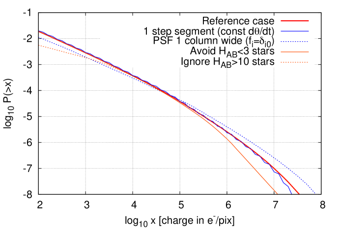
Figure 2: Comparison of stimulus levels predicted under different assumptions and approximations. The vertical axis shows the log probability to exceed a given stimulus level during a slew of 0.4 degrees (a step along the short axis of the field, executed frequently during the HLS). The thick red line indicates reference assumptions. The solid blue line treats the slews as being at constant $\dot{\theta}$. The dashed blue line approximates the PSF as 1 column wide (all the flux from the star is concentrated in the central column). The orange lines show what happens if bright ($H_{\rm AB}<3$) or faint ($H_{\rm AB}>10$) stars are excluded from the model.

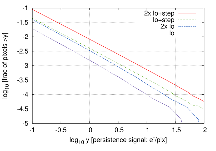
Figure 3: The cumulative distribution function of slew-induced persistence in the HLS imaging survey, $P(>y)$. The persistence signal $y$ is estimated in electrons per pixel; the decaying persistence curve is integrated over a 160 s. Several persistence models are shown, including the “lo” case (typical of the development detectors), and a “lo+step” case (including an order of magnitude step at saturation, as seen in portions of some detectors). This figure has not been updated yet to go from the 6-year to the 5-year observing plan, although we expect only minor differences.

After negotiating with the Project, we settled on a mitigation strategy for slew persistence that involved saving the spacecraft orientation information from the Attitude Control System (ACS), using this to predict the locations of persistence from bright star streaks, and masking $\pm 2\sigma$ on either side of these streaks. Unmasked streaks are simply accepted as part of the systematic error budget. Their impact on shape measurement is based on an analytic result derived by our SIT and tested against Monte Carlo simulations:

$$\Delta\gamma_{1}+i\Delta\gamma_{2}=\frac{M\Omega_{\rm max}\sigma_{\rm n}^{2}R^{4}}{2F^{2}N_{\rm ind}\,{\rm Res}}f_{\rm scale}f_{\rm aniso},$$ (12)

where $\Delta\gamma_{1,2}$ are the two components of spurious shear; $M$ is a margin factor; $\Omega_{\rm max}=421.3$; $\sigma_{\rm n}^{2}$ is the variance of the persistence image; $R$ is the radius of the galaxy in pixels; $F$ is the signal from the galaxy in electrons per exposure; $N_{\rm ind}$ is the number of independent exposures of the galaxy; Res is the galaxy resolution factor Bernstein and Jarvis (2002); $f_{\rm scale}$ and $f_{\rm aniso}$ are factors $\leq 1$ describing the scale dependence and anisotropy of the persistence power spectrum (defined to be 1 in the worst case).

The results of this study – shown in Figure 4 – are promising, given the top-level systematic shear budget of $2.7\times 10^{-4}$ and that the modern detectors typically show “lo” or (in some regions) “lo+step”-like behavior, rather than the much larger persistence characteristic of the WFC3-IR model (third column). The masking algorithm will continue to be revisited as part of the mission optimization. However, the small number of masked pixels led the FSWG to conclude that a dark shutter that operated during every slew was not required for the WFIRST HLS.

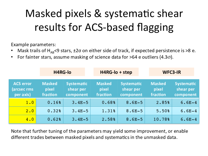
Figure 4: The outcome of the October 2016 slew persistence study. This shows the masked pixel fraction and the predicted systematic shear due to unmasked streaks as a function of both the persistence model and the accuracy of pointing information.

We carried out a related study, also using Eq. (12) and related machinery, to assess how well we need to know the dark current for WFIRST. Dark current measurements without a dark filter are possible, e.g. via median algorithms that combine many exposures from a survey, but are subject to: (i) a degeneracy in which the “true” sky brightness is unknown and hence the zero level of the dark current cannot be established, and (ii) possible correlated errors from imprinted celestial sources. The requirements, as derived in the appendix to the calibration plan, are:

• The error in the dark current + bias determination in a 140 s HLS imaging exposure shall be no more than $0.0096f_{\rm corr}^{-1/2}$ e/p/s (uncorrelated part) or $0.0017f_{\rm corr}^{-1/2}$ e/p/s (imprinted celestial sources).

• The error in the dark current + bias determination in a 297 s HLS spectroscopy exposure shall be no more than $0.0059f_{\rm corr}^{-1/2}$ e/p/s (uncorrelated part) or $0.00072f_{\rm corr}^{-1/2}$ e/p/s (imprinted celestial sources).

Here “$f_{\rm corr}$” denotes the factor by which we plan to correct biases induced by errors in the dark current map (we normally choose $f_{\rm corr}=1$ to be conservative). The requirements are traceable to additive shear biases from non-circular imprinted celestial sources; multiplicative shear biases as the noise in the dark current map results in e.g. galaxy centroids getting “pulled” toward pixels whose measured dark current fluctuates below the true dark current of that pixel; and Eddington-like biases for sources detected in the GRS. While the semi-analytic estimates in the calibration plan based on source counts suggest that the HLS imaging requirement can be met without a dark filter, our SIT and the Calibration Working Group had concerns about possible degeneracies in the self-calibration procedure that can only be addressed by a detailed simulation. Moreover, the approach requires empty space in the images, which we will not have in the case of grism spectroscopy. As the imaging exposures are shorter than the spectroscopy exposures, this would require dedicated long imaging exposures (of HLS spectroscopy exposure length) just for the purpose of self-calibrating the dark. Due to sky Poisson noise, we would need many of these images – our Feburary 2017 estimate was for $N=73$ exposures, which, if done every week, would consume 4% of the wall clock time. In light of these and other issues, the Calibration Working Group recommended that WFIRST maintain the dark filter.

4.2.2 Calibration Plan

Our SIT has contributed extensively to the WFIRST WFI Calibration Plan. This includes extensive quantitative analysis of proposed calibration techniques, as detailed in the appendix to the plan. Some highlights follow.

The requirement on knowledge of the dark current and the calibration approaches are fully defined, based on analysis done during the dark filter trade (October 2016 – February 2017).

Weak lensing was found to place demanding requirements on measurement of the count rate-dependent non-linearity (CRNL). The weak lensing program is sensitive to CRNL because it enhances the bright center of a PSF star relative to its wings, thereby making the star appear slightly smaller, but does not have a similar effect on the faint galaxies used for shape measurement. The PSF second moment is biased by a factor of $1-\alpha$ (where $\alpha$ is the CRNL exponent), and has a top-line systematic error budget of $7.2\times 10^{-4}$. This means that if $\alpha$ is measured to $\pm 3\times 10^{-4}$ (the requirement from the supernova SITs), then CRNL consumes 17% of the PSF size error budget, in an RSS sense. Given that CRNL is a pernicious bias for two of the dark energy probes, we recommended a multi-faceted approach to CRNL calibration, including a lamp-on/lamp-off capability for WFIRST (this was not available on WFC3-IR).

Our team has revisited the wavefront stability requirements for weak lensing, using a set of codes and scripts on the team’s GitHub site. This begins with a Fisher matrix analysis of the uncertainties in the shear power spectrum, and our top-line requirement that the systematic errors be equivalent to the statistical errors even if the survey is extended to 10,000 deg² (i.e. in an RSS sense, the systematic errors should be 20% of the statistical errors in the nominal 2,000 deg² survey). Requirements are assessed using the significance, defined by

$$Z=\sqrt{\Delta{\bf C}\cdot{\bf\Sigma}^{-1}\Delta{\bf C}},$$ (13)

which is the number of sigmas at which one could distinguish the correct power spectrum from the power spectrum containing a systematic error. We built sub-allocations for multiplicative (shear calibration) errors, and for additive (spurious shear) errors in each angular bin. An early discovery was that this process depends on the redshift dependence of the shear error: some redshift dependences are “worse” than others by the $Z$-metric. The worst possibility is not for the error to be redshift-independent, but rather for it to change sign, as this can mimic a change in redshift evolution of the growth of structure.

In our current formalism, for each angular template, we introduce a limiting amplitude $A_{0}^{\rm flat}(\alpha)$, defined to be the RMS spurious shear per component $A_{0}$ at which we would saturate the requirement on $Z(\alpha)$ for angular bin $\alpha$ in the case of a redshift-independent systematic $w_{i}=1\,\forall i$ (here $\alpha$ denotes an angular bin and $i$ a redshift bin). That is, if the additive systematics did not depend on redshift, we could tolerate a total additive systematic shear of $A_{0}^{\rm flat}$ (RMS per component) in band $\alpha$. We also introduce a scaling factor $S[{\bf w},\alpha]$ for a systematic error

$$S[{\bf w},\alpha]=\frac{Z(\alpha)\,{\rm for\,this\,}w_{i}}{Z(\alpha)\,{\rm for\,all\,}w_{i}=1}$$ (14)

that depends on the redshift dependence $w_{i}$. An additive systematic error that is independent of redshift will have $S=1$. A systematic that is “made worse” by its redshift dependence will have $S>1$, and a systematic that is “made less serious” by its redshift dependence will have $S<1$. The requirement that the (linear) sum of $Z$s not exceed $Z(\alpha)$ thus translates into

$$\sum_{\rm systematics}[A(\alpha)]^{2}\times S[{\bf w},\alpha]\leq[A_{0}^{\rm flat}(\alpha)]^{2},$$ (15)

where $A(\alpha)$ is the RMS additive shear per component due to that systematic. We take the “reference” additive shear to be the additive shear in the most contaminated redshift slice; in this case, $w_{i}=1$ for that slice, and $|w_{i}|\leq 1$ for the others. Under such circumstances, we can determine a worst-case scaling factor $S_{\rm max,\pm}(\alpha)$, which is the largest value of $S[{\bf w},\alpha]$ for any weights satisfying the above inequality. We may also determine a worst-case scaling factor $S_{\rm max,+}(\alpha)$ conditioned on $0\leq w_{i}\leq 1$, i.e. for sources of additive shear that have the same sign in all redshift bins. In most cases, however, something is known about the redshift dependence of the systematic error (e.g. for PSF errors the error scales with the size of the galaxy, and hence has a redshift dependence tied to the measured redshift evolution of galaxy sizes). In these cases, we use the correct redshift weighting factor $S$. This approach has been critical in order to set stability requirements that are consistent with the Project’s integrated modeling results.

We have begun incorporating the HLS observing strategy (§7) in studies of self-calibration of time-dependent drifts in the response of the system (i.e. time dependence of the conversion from $\mu$Jy on the sky to DN/s in the digitized detector system outputs). This model is in a state of flux as we add parameters to it, but here we show a current snapshot allowing for time-dependent drifts of the response of each of the 18 SCAs making up the focal plane, with time dependence parameterized in calibration periods of $\Delta t$ (assessed down to a period of 3 hours) each. Both individual-SCA drifts and common-mode drifts are allowed, with an assumed intrinsic variation (calibration prior) of 1% RMS drift in each $e$-fold of timescales. A network of randomly distributed stars with a density of 500 stars/deg² and $S/N=50$ was assumed; in self-calibration, the magnitudes of these stars are not known a priori, but are assumed to be stable across multiple repeated observations of the same field. These are preliminary parameters being used to test our tools and are not currently held as requirements. The stellar density model is very conservative since the Trilegal model predicts star counts of 572, 803, 990, and 1137 stars/deg² at $H_{\rm AB}=18-19$, $19-20$, $20-21$, and $21-22$ at the SGP, and even an $H_{\rm AB}=22$ star will have $S/N>50$. The temporal stability of the system needs further study and will be varied as an input parameter in future versions of this model. The current model uses the April 19, 2017 update to the HLS observing strategy. The number of calibration parameters varies depending on the filter, since there are no parameters for periods of time when the instrument is not observing in that filter; the current version has 17262 parameters for the H band.

Despite the intrinsic stability assumed, in which each SCA can have its response fluctuate by 1.67% RMS from one time interval to the next, the repeated observations do an excellent job of tracking these changes and reducing the posterior uncertainty. Even for $\Delta t=0.125\,$days$=3\,$hours, the posterior calibration errors are at the level of 0.14–0.17% RMS (here “RMS” is weighted by number of observations), depending on the filter. An example of the model output (predicted uncertainties in the calibration parameters for each SCA at each epoch) is shown in Figure 5. It must be remembered that this analysis is overly simplistic in some ways – particularly that we have not yet allowed for shorter-timescale variations (i.e. on timescales $<\Delta t$), nor have we allowed for separate gain drifts among the different readout channels. These will have to be included in a future version of the model. On the other hand, the stellar density and $S/N$ assumptions were extremely conservative (e.g. the full range of stellar magnitudes 18–22 should have 7 times more stars than were assumed, even at the Galactic pole), so there is margin to absorb these additional degrees of freedom. The next iteration of the model for time-dependent calibration drifts will include additional parameters, as well as updated priors reflecting expected detector system stability rather than the place-holder requirements shown here.

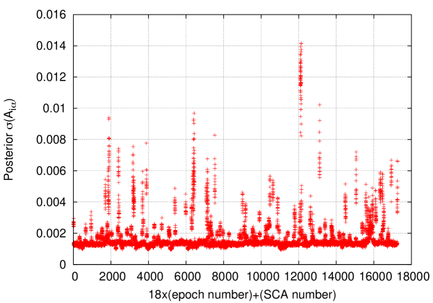
Figure 5: An example of the posterior calibration error from an HLS self-calibration calculation. The horizontal scale displays the time intervals (left-to-right in time order), with 18 points per time interval indicating the various SCAs. The vertical axis shows the standard deviation of the calibration solution for that SCA at that time, $\sigma(A_{i\alpha})$, relative to the survey mean. The figure shows the case of H band with $\Delta t=0.125$ days. This example had 17262 calibration parameters. A few epochs, mostly containing only a few observations, are poorly constrained due to minimal overlap observations. It is subject to refinement and the input parameters of the model will be varied as we work toward requirements on the stability of the detector system.

4.3 Identifying and Studying the Effect of Detector Imperfection (D3, D7)

Since precision cosmology measurements depend sensitively on exquisite photometry; subtle effects that might not be noticeable in other areas of astrophysics can become important when trying to measure galaxy shapes to $<0.1$%. Over the past year, we have studied novel possible systematic effects, implemented in an image simulation pipeline new and known effects and released it to the community. Our goal is to derive requirements for all these effects. Highlights include

1. The study of the effect of polarization-dependent quantum efficiency;

2. The requirements on the interpixel capacitance;

3. Detector characterization;

4. Image simulation including detector imperfection and WFIRST scanning strategy to study their effect on shape measurement.

In what follows, we provide some highlights from our detector characterization and simulation activities.

4.3.1 Polarization Effects

During early 2017, work was carried out to assess the approximate level of an effect that could cause weak lensing systematics, but that had never been previously considered by the weak lensing community. This effect is polarization-dependent quantum efficiency (due to e.g. different reflectivity of various coatings for different polarizations of light). Since the light from edge-on disk galaxies typically has some low level polarization perpendicular to the disk, any polarization-dependence of the QE could result in a preferential selection of such galaxies based on their orientation in the focal plane. This would violate the baseline assumption in a weak lensing analysis, which is that all coherent galaxy alignments are due to gravitational lensing.

A student at CMU, Brent Tan, worked with Rachel Mandelbaum and Chris Hirata on a simple toy model for this effect. The toy model had two parameters: the fraction of the disk galaxy light that is polarized, and the relative attenuation of that perpendicular polarization component (both numbers in the range $[0,1]$). For each point in that parameter space, the coherent shear due to selection bias was calculated; see results in Figure 6. Finally, the results were modified to account for the fact that not all disk galaxies are viewed edge-on and that not all galaxies are disks, giving a net coherent shear due to this selection bias of $\sim 3\times 10^{-4}$. The results are still quite uncertain because our fiducial values for the disk polarization fraction were based on observations of nearby galaxies, not $z\sim 1$ disks. However, this is large enough to be relevant for WFIRST, so this systematic needs to be evaluated more carefully and requirements placed in future. A publication on this topic will be prepared during summer 2017.

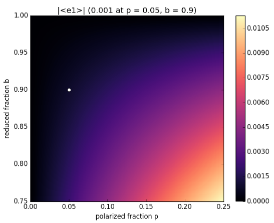
Figure 6: The average shear due to weak lensing selection biases due to polarization-dependent quantum efficiency, as a function of the fraction of polarized light from edge-on disks (horizontal axis) and the fractional attenuation of the perpendicular polarization (vertical axis). The dot at $(0.05,0.9)$ is our fiducial point in parameter space, and has $\langle e\rangle\approx 0.001$.

Another possible polarization-related systematic is a polarization-dependent PSF. That will be the subject of future work.

4.3.2 Interpixel Capacitance Requirements

The WFIRST detectors will suffer from electrical crosstalk between the pixels, unlike the optical detectors that are based on CCDs. This effect, known as the interpixel capacitance (IPC), appears as a systematic effect in the weak lensing shear measurements and causes a bias in the measurements if not properly taken into account. The effect of IPC on the point-spread function (PSF) was already studied by members of our SIT in Kannawadi et al. (2016), and requirements were placed on the level of uncertainty in the IPC based on how that uncertainty affects the PSF.

More recently, in late 2016, members of our SIT (Mandelbaum and student Kannawadi) carried out and analyzed simulations to determine whether additional requirements on IPC are needed to ensure that weak lensing shear estimation is not biased beyond our tolerances. To calibrate the shear multiplicative bias to an accuracy of $2\times 10^{-3}$, we find that the requirements on the IPC placed by the PSF requirements are sufficient, so no new requirement is needed. A paper on this result is in preparation.

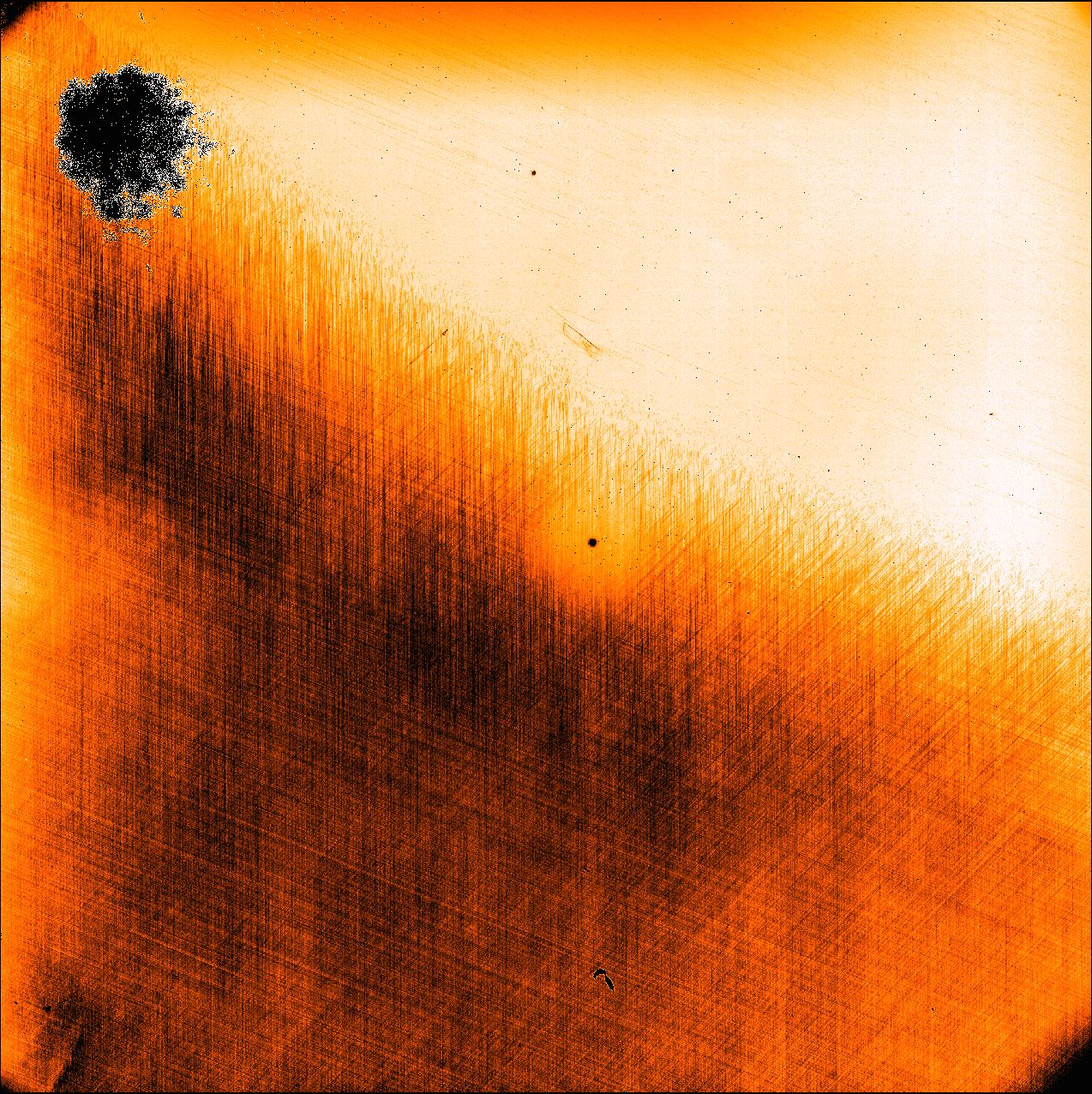
Figure 7: 2048 x 2048 flat-field calibration image taken with a Euclid engineering grade H2RG detector (2.4 $\mu$m cutoff) under 1 $\mu$m illumination (scaled to enhance contrast). Flight detectors resemble the upper right region (mean QE $\sim$ 1) but still contain traces of the “crosshatch” pattern visible in the lower left (mean QE $\sim$ 0.8). Scanning a grid of undersampled point sources (f/11 aperture setting) in sub-pixel increments generated 1% RMS photometric variations in the lower left region which were not removed by the flat-field calibration. This result provides evidence that the pattern has intra-pixel structure that potentially biases the PSF if left uncalibrated.

4.3.3 Laboratory Detector Characterization

The WFIRST dark energy analyses will place enormous demands on our understanding of the detectors. Some aspects of this problem can be anticipated in advance – for example, we know that effects such as inter-pixel capacitance, count-rate-dependent non-linearity will need to be carefully characterized, and we are working as part of the Calibration Working Group to build these measurements into the mission (collaborator Shapiro is co-leading this particular Working Group). However, with systematic error budgets at the level of a few$\times 10^{-4}$, it is likely that WFIRST analyses will turn up new effects that were not apparent in past missions. Therefore a key task for our SIT is to analyze the data from development detectors and identify these new effects early enough to inform the calibration plan.

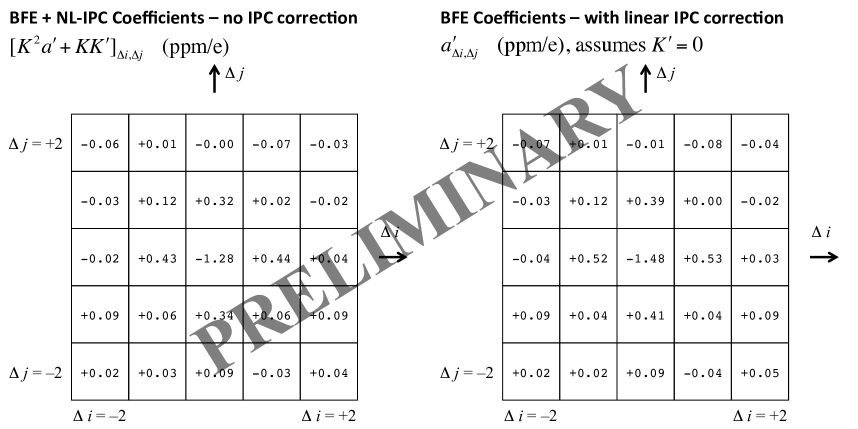
Figure 8: The BFE + NL-IPC coefficients $[K^{2}a^{\prime}+KK^{\prime}]_{\Delta i,\Delta j}$ (left panel) and IPC-corrected coefficients $a^{\prime}_{\Delta i,\Delta j}$ (right panel), for H4RG-17940. Note that the IPC-corrected coefficents assume that the IPC is linear, i.e. the non-overlapping correlations are ascribable entirely to the BFE and not NL-IPC. The $1\sigma$ uncertainty in each pixel is 0.07 ppm/e.

In ground-based weak lensing projects using thick CCDs (e.g. DES), one of the key detector issues has been the brighter-fatter effect (BFE). This is an electrostatic effect in which as a pixel fills up with collected charge, it changes the electric field geometry and new charges generated are more likely to be deflected into neighboring pixels. This has the effect of making bright stars appear larger than faint stars, as the repulsion effect is non-linear and increases with signal level. The field geometry is very different in a NIR detector, but a brighter-fatter effect is still possible. Plazas et al. (2017a) and Plazas et al. (2017b) report a first detection of the BFE in NIR detectors (H1RG and H2RG) using on-sky and laboratory data, respectively.

We have searched for the brighter-fatter effect in the H4RG detector arrays using the flat fields for two devices H4RG-17940 and H4RG-18237, provided to us by the DCL. The BFE imprints a signature in the auto-correlation function of a flat field; using the correlations in multiple non-destructive reads in a flat field, one can separate linear IPC from the BFE. Preliminary brighter-fatter effect results for H4RG-17940 are shown in Figure 8. The BFE coefficients are $a^{\prime}_{\Delta i,\Delta j}$, which is the fractional change in effective area of pixel $(i,j)$ when an electron is placed in pixel $(i+\Delta i,j+\Delta j)$; they have units of parts per million per electron (ppm/e). The flat auto-correlations are sensitive to both the brighter-fatter effect and non-linear inter-pixel capacitance (NL-IPC); we are currently working on distinguishing the two effects.

We are also using data from studies of more mature H2RG detectors to inform our calibration plan. Although these will have important differences from the WFI flight detectors, we expect that problematic effects discovered in H2RGs will need to be characterized in H4RGs at some level. For instance, collaborators Shapiro and Huff (via the Precision Projector Laboratory at JPL directed by collaborator Shapiro) have investigated a high-frequency pattern (dubbed the “crosshatch”) apparent in flat-field calibrations and believed to be related to the crystal structure of HgCdTe (see Figure 7). Using an engineering grade H2RG provided by the Euclid mission, tests have shown that the crosshatch pattern affects photometry even after flat-field calibrations are applied, implying that it has sub-pixel structure that can bias PSF measurements. Data was shared with this SIT to investigate the dependence of the pattern on polarization and angle of incidence. The same H2RG detector is also being used to conduct a PSF-based test of BFE to compare with our flat-field analysis.

4.3.4 Simulating Detector Imperfection and Their Effect on WFIRST Shape Measurements

Building on the existing GalSim framework and WFIRST module, Michael Troxel and Ami Choi (in collaboration with Hirata, Jarvis, and Mandelbaum) are developing an image simulation pipeline to assess the impact of various physical effects on the fidelity of the measured galaxy shapes. The end product will provide realistic simulations containing all pertinent effects and conditions from the observational process specific to the WFIRST mission that may affect the quality of the lensing shear extracted from the real WFIRST images. These simulations will provide a foundation to characterize the relative impact of undesired effects and to validate the shear measurements themselves. As the distribution and density of galaxies are realistically incorporated, the resulting multi-epoch images can also be used to test different dither strategies. An intermediate level goal is to update the module with the most recent hardware and survey parameters describing the mission, to do some GalSim development to make the pipeline more efficient, and to estimate the relative impacts from detector effects such as the IPC described in earlier sections.

The pipeline is currently capable of simulating galaxies on individual postage stamps with a size and flux distribution drawn from the CANDELS catalog from Capak and Hemmati, a dither pattern from Hirata, realistic noise (see below), correct layout of SCAs, and options to dial a range of detector-level effects such as IPC, non-linearity, and reciprocity, among others. The output simulated galaxies and truth tables are saved in Multi Epoch Data Structures (MEDS), which is a format commonly used in DES. A publicly available shape measurement software, ngmix (), has been interfaced to measure shapes of the simulated galaxies. Figure 9 illustrates a few of the effects in the context of a simulated bright, elliptical galaxy on a 32x32 pixel postage stamp. The software is maintained in a repository available at on GitHub.

The H4RG read noise model developed by Rauscher (2015) can be straightforwardly incorporated into the simulations in order to study the effects of correlated noise on shape measurement. Hirata has used simulations and a semi-analytic formalism to show that anisotropic noise induces additive ellipticity measurement errors, with the most damaging contributions coming from noise power at spatial wavelengths $\sim\pi R$ where $R$ is the observed scale radius of the galaxy or star. With these tools, we will be able to derive requirements on detector noise and calibrate shape measurement pipelines to correct for remaining correlated noise.

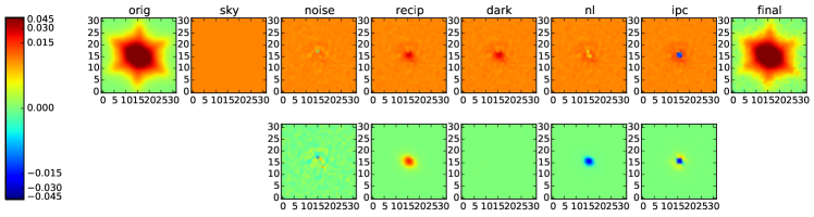
Figure 9: An example of a simulated bright, elliptical galaxy produced by the image simulation pipeline. The top row of subpanels begins with the original simulated bright elliptical galaxy (far left). Each subpanel to the right of the original galaxy is a “difference” image that has the original galaxy subtracted off after the given effect (top label) has been applied. These effects are: sky background, noise, reciprocity, dark current, nonlinearity, inter-pixel capacitance, respectively. The bottom row of subpanels corresponds to the individual, isolated effects (top label). The top, far right subpanel shows the final galaxy image after all effects have been applied. The sub panels have been normalized by the maximum flux value of the original galaxy image, and the colors have been mapped to $\log_{10}$ values with a small range right around zero mapped to linear values as shown on a single colorbar corresponding to all of the subpanels.

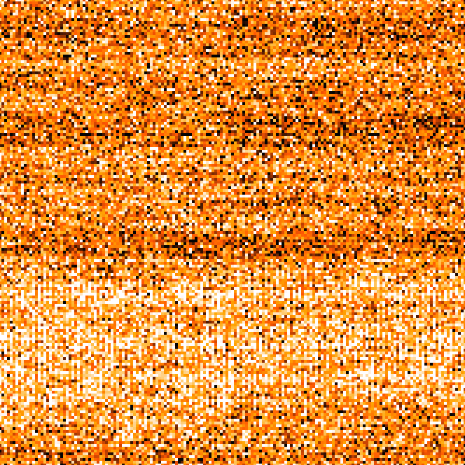
Figure 10: LEFT: Simulated noise in an H4RG subregion using the model of Rauscher (2015). This image demonstrates the spatial effect of 1/f noise (horizonal bands) and alternating column noise (high frequency vertical striping). RIGHT: Weight function showing the relative contribution of noise with spatial wavenumber $k$ to the ellipticity bias of a source with scale radius $R$. For a given signal to noise level, the read noise shown would bias $e_{1}$ by different amounts for an undersampled PSF versus a larger galaxy. This weight function assumes an adaptive moments shape measurement algorithm.

4.4 Enabling Photometric Redshifts with WFIRST (D6, D11)

Accurate photo-$z$s are crucial to all WFIRST probes of dark energy. In the first year of SIT activity we have focused on developing accurate data-driven simulations of the WFIRST lensing galaxy population and determining the requirement on the spectroscopic samples needed to calibrate these photometric redshifts. We proposed a plan to calibrate this sample and study the importance of the IFC. In the process, we generate new data products that we released to other SITs and to the community.

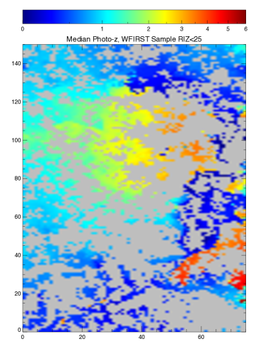
Figure 11: A Self Organizing Map (SOM) (Masters et al., 2015) of color space generated from $\sim 6$ square degrees of data in the VVDS 2h, SXDS/UDS, COSMOS, and EGS survey areas colored by photometric redshift is shown. Only regions occupied by the CANDELS survey are colored, with the remaining area grey. CANDELS only covers 42% of the color space, representing 49% of the overall galaxy population.

4.4.1 Generating Data-driven Simulations of WFIRST Galaxy Population

The closest analogs to WFIRST data are the COSMOS and CANDELS HST surveys, however neither is fully analogous to WFIRST HLS data. The COSMOS data cover 1.7 square degrees with HST-ACS (F814W) with ground based data analogous to LSST. However, WFIRST analogous infrared data are not available over the majority of the field and extrapolations to the WFIRST lensing cuts from the F814W data over-estimate the number-density of sources usable for lensing. In contrast, CANDELS has WFIRST analogous infrared data, but covers only 0.2 square degrees,which means it does not sample the full WFIRST galaxy population, and has very heterogeneous optical coverage. Specifically, a comparison between the CANDELS and COSMOS data to R,I,Z$<$25 found that only 42% of COSMOS galaxy colors (representing 49% of the galaxy population) are present in CANDELS. Figure 11 shows a Self Organizing Map (SOM) (Masters et al., 2015) of the galaxy color space with regions where CANDELS galaxies fall marked. The empty regions are shown in grey and correspond to cells with low galaxy density in COSMOS. So these galaxies are simply less likely to be found in the relatively small area of CANDELS.

To overcome these limitations we have taken several approaches. First, we have collected a homogeneous 0.3-2.5$\mu$m data set over $\sim 6$ square degrees in the VVDS 2h, UDS/SXDS, COSMOS, and EGS fields. These data are not as deep as WFIRST, but are analogous to the LSST and Euclid data and allow us to estimate the cosmic variance in galaxy population and estimate requirements on spectroscopy. These have been combined with the CANDELS catalogs which probe WFIRST depth but are sample size and variance dominated. We then adapted the simulations described in Stickley et al. (2016) developed for the SPHEREx mission to assign a R$\sim$600 spectra to each object. The CANDELS data are very heterogeneous (see Table 1), so we converted the various photometric systems to a LSST+WFIRST system. Figure 12 shows an example of the LSST+WFIRST system along with the CANDELS filters on GOODS-S as an example. For the conversion we compared the converted photometry from other bands to actual CFHT-LS $u^{*}$, $g^{*}$, $r^{*}$, $i^{*}$, $z^{*}$ and VISTA $Y$, $J$, $H$, $K_{s}$ photometry in fields where they are available. We found a simple linear interpolation between filters in flux produced the best agreement. Using the Stickley et al. (2016) or other template fits produced discretized value in the output fluxes which biased further analysis.

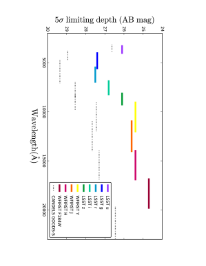
Figure 12: The 5$\sigma$ limiting AB magnitude of LSST and WFIRST filters plotted as solid color lines and the 5$\sigma$ limiting AB magnitude of CANDELS GOODS-S filters are plotted with dotted black lines (see Table 1 for filter names). Note the significant differences in the filter system which necessitates conversion from one to the other.

The combination of these catalogs produces a reasonable estimate of the WFIRST galaxy population for the purposes of assessing variance and the effects of cuts. However for some analysis a fully simulated catalog is required so that the inputs are known perfectly. To provide this we further adapted the methods described in Stickley et al. (2016) to produce simulated WFIRST+LSST photometry. These three sets of simulated samples are being provided to other WFIRST SIT teams for their analysis. Specifically we have been working with the Foley SNe focused SIT team to simulate photo-$z$ performance for supernova cosmology.

Table 1: CANDELS filters in each field used to create the LSST+WFIRST catalog

Field							Filters
GOODS-S	$\rm U_{VIMOS}$	$\rm F435W$	$\rm F606W$	$\rm F775W$	$\rm F814W$	$\rm F850lp$	$\rm F098W$	$\rm F105W$	$\rm F125W$	$\rm F160W$	$\rm Ks_{HAWK-I}$
GOODS-N	$\rm U_{KPNO}$	$\rm F435W$	$\rm F606W$	$\rm F775W$	$\rm F814W$	$\rm F850lp$	$\rm F105W$	$\rm F125W$	$\rm F160W$	$\rm Ks_{CFHT}$
EGS	$\rm U_{CFHT}$	$\rm g_{CFHT}$	$\rm F606W$	$\rm r_{CFHT}$	$\rm i_{CFHT}$	$\rm F814W$	$\rm z_{CFHT}$	$\rm F125W$	$\rm F160W$	$\rm Ks_{CFHT}$
UDS	$\rm U_{CFHT}$	$\rm B_{subaru}$	$\rm F606W$	$\rm Rc_{subaru}$	$\rm i_{subaru}$	$\rm F814W$	$\rm z_{subaru}$	$\rm Y_{HAWK-I}$	$\rm F125W$	$\rm F160W$	$\rm Ks_{HAWK-I}$
COSMOS	$\rm U_{CFHT}$	$\rm B_{subaru}$	$\rm F606W$	$\rm r_{subaru}$	$\rm i_{CFHT}$	$\rm F814W$	$\rm z_{CFHT}$	$\rm Y_{UVISTA}$	$\rm F125W$	$\rm F160W$	$\rm Ks_{UVISTA}$

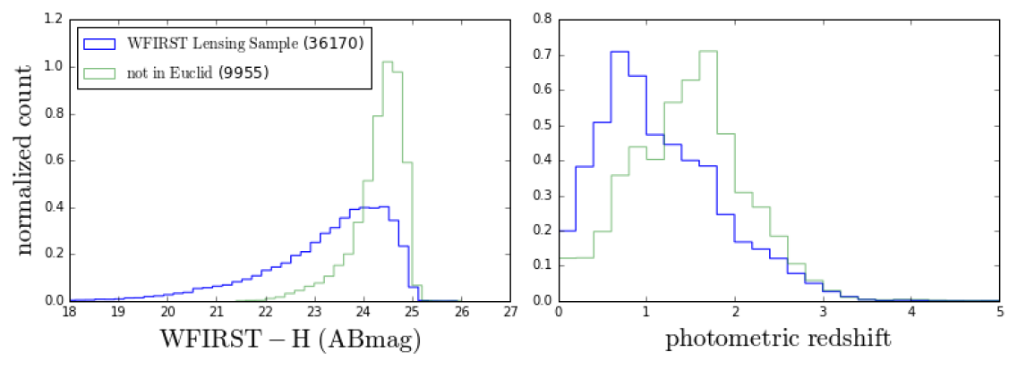
Figure 13: Left: A magnitude histogram of the WFIRST lensing sample split into a C3R2 Euclid like lensing sample (blue, $RIZ<25$) and those only in WFIRST (green). Roughly 20% of the WFIRST sample consists of galaxies fainter than what C3R2 is calibrating for Euclid. Note the Euclid lensing sample is cut at $RIZ<24.5$, shallower than the proposed calibration (Masters et al., 2015). Right: The redshift distribution of the C3R2-Euclid sample (blue) and the WFIRST only sample (green) are shown normalized to an integral of 1. Even though the WFIRST galaxies are fainter than the calibration limit they cover a redshift range similar, just with with more galaxies at high-redshift.

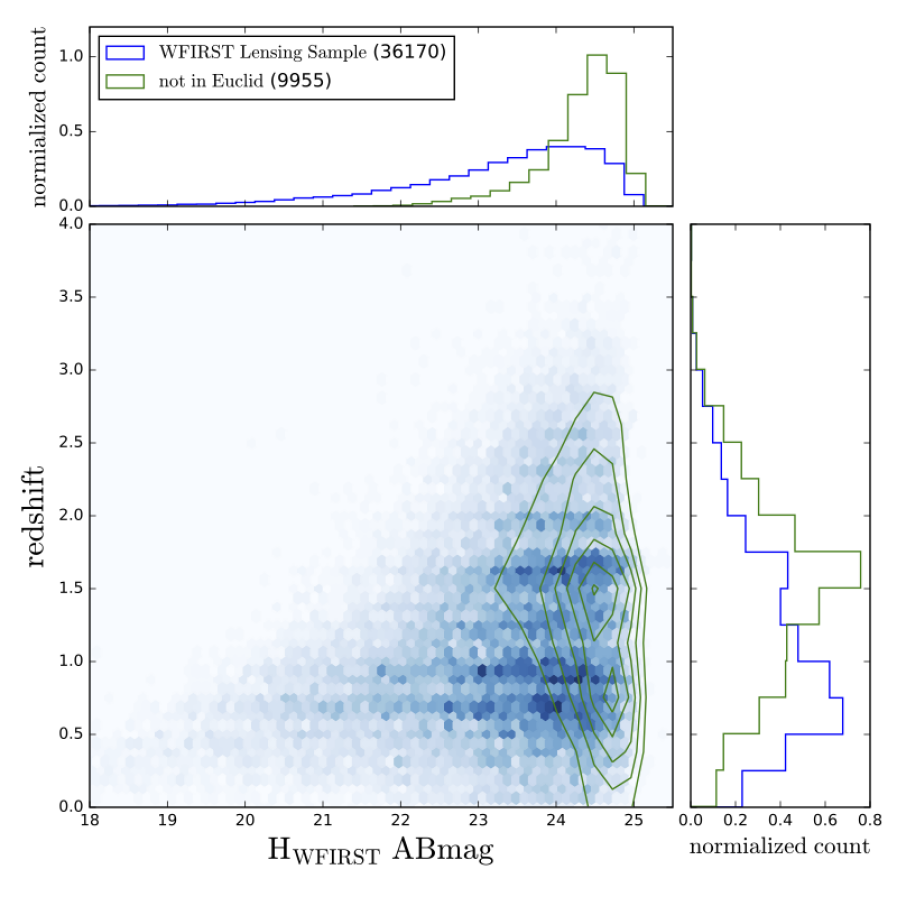
Figure 14: $H$ band magnitude vs redshift is plotted for the WFIRST lensing sample shown in Figure 13 with shading indicating relative density. The WFIRST only sample shown as green contours and the histograms from from Figure 13 are plotted on the axis.

4.4.2 Calibrating the Photometric Redshifts of WFIRST Weak Lensing Galaxy Population

These simulations have been used for several analyses within our SIT. Figure 13 shows the relative differences in the magnitude and redshift distribution of the total Euclid and WFIRST faint lensing samples. WFIRST clearly adds fainter and higher-redshift systems to the weak lensing sample. However, Figure 15 shows a Self-Organizing-Map analysis (Masters et al., 2015) of the WFIRST lensing sample compared with the Euclid sample. Even though WFIRST is significantly fainter than Euclid, 96% of galaxies fainter than the Euclid sample have color analogs at brighter magnitudes. The implication is that while WFIRST is seeing fainter galaxies than Euclid, these galaxies are very similar to less numerous but brighter systems seen by Euclid.

Figure 15: A Self Organizing Map (SOM) (Masters et al., 2015) of the WFIRST color space based on the CANDELS data cut to the WFIRST lensing sample color coded by their median redshift. The left panel shows SOM cells that contain galaxies too faint to be in the C3R2 RIZ$<25$ Euclid like sample (Masters et al., 2015, 2017). The right panel shows SOM cells with galaxies that are in the C3R2 sample. $\sim 96\%$ of the WFIRST color space is occupied by galaxies in the C3R2 sample, however $\sim 20\%$ of the WFIRST sample is fainter than the C3R2 limit. This means their calibration would have to be verified to ensure no magnitude dependence on redshift.

To determine how difficult it would be to obtain spectra for these faint systems we conducted an analysis of the R$\sim$600 SEDs fit to the photometry. Based on the C3R2 survey spectra (Masters et al., 2017) we developed a spectral simulator which accurately re-produces ground based spectra for Keck DEIMOS, LRIS, and MOSFIRE. In addition to these instruments the simulated response of the WFIRST-IFC was simulated. Example simulated spectra based on the model fits along with actual Keck spectra obtained for those sources are shown in Figure 16.

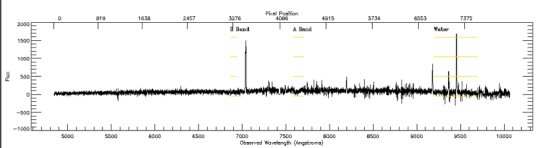
Figure 16: A real (top) and simulated (bottom) spectra of a $I=22.7$ galaxy in the C3R2 sample.

We found that indeed most of the faint WFIRST lensing galaxies were analogs of brighter systems. This alleviates the need to obtain spectroscopic redshifts to this population since the color-redshift relation will be known. However, steps must be taken to validate that the redshift distribution does not change at fainter magnitudes in ways not apparent in the WIFRST+LSST colors.

The simplest method would be to extend a survey such as C3R2 (Masters et al., 2017) to fainter magnitudes. However, these faint galaxies are difficult to obtain high-quality spectra for from the ground. For the purposes of this analysis we define high quality as an SNR$>$7 on two emission features or an SNR$\sim 5$ on an underlying continuum. Based on this criteria, 20% of the WFIRST color space requires $>5$h spectra from Keck. It is important to note this is in terms of color space, and the exact number of spectra required to calibrate this color space will require further analysis. Of these, 1% are sources that require long ground exposures due to strong emission lines falling between ground based observing windows and spectra could be obtained with the WFIRST grism. A further 15% would have high-quality redshifts with WFIRST-IFC parallel observations based on simulating the spectra and assessing the number of features with SNR$>$7. However, due to the low-resolution of the WFIRST-IFC further analysis may be merited. The remaining 4% of galaxies could not be calibrated by WFIRST or from the ground with 10m telescopes and would require either ELTs or JWST.

4.5 Cluster Cosmology with WFIRST

Our work during the past year has focused on building machinery for comprehensive cosmological forecasts for the WFIRST cluster program that will include representations of the most significant anticipated systematic effects.

Cluster cosmology is generally considered to be less demanding in terms of hardware requirements than cosmic shear, since the large galaxy over-densities and shear signals are not as easily masked by subtle optical aberrations or detector behaviors. Nevertheless, it may place new requirements on survey footprint/operations (to ensure overlap with other data sets); pipeline behavior in crowded fields (e.g., Simet and Mandelbaum (2015)); and ancillary data products and simulations to describe, e.g., changes in selection effects and source redshift distributions in the presence of blending and magnification.

Clusters can be identified using galaxy counts in WFIRST and external data, or from X-ray or Sunyaev-Zeldovich surveys. WFIRST yields high-precision measurements of cluster weak lensing shear profiles, which can be combined with cluster abundances and cluster-galaxy cross-correlations to derive cosmological parameter constraints, most notably on the amplitude of matter clustering.

We have verified our ability to reproduce previous forecasts quantitatively with new and independent code – a non-trivial exercise that required resolving ambiguities about halo mass definitions, source redshift distributions, and so forth. We have extended the new code so that it can simultaneously model weak lensing signals from small scales (the “one-halo” regime) out to large scales described by linear theory. To achieve accurate results in the transition between these regimes, we have developed a numerically calibrated prescription for mass profiles in the “splashback” zone beyond the cluster virial radius. These numerical calibrations are based on a suite of cosmological N-body simulations that we are using to create full numerical “emulators” for cluster-mass and cluster-galaxy cross-correlation functions, using parameterized halo occupation distributions to relate galaxy populations to the underlying dark halo population. We are exploring the degree to which cluster-galaxy cross-correlations can sharpen cosmological constraints when combined with cluster weak lensing; we anticipate including these cross-correlations in our cosmological forecasts at a later time.

Our current focus is on incorporating a realistic description of photometric redshift distributions and nuisance parameters that describe systematic uncertainties in those distributions. Our hope is that the combination of cosmic shear and cluster weak lensing measurements will prove much more robust to photometric redshift uncertainties than either technique individually, because the two methods have somewhat different dependence on source redshifts, and because the redshifts of the clusters themselves are accurately known. We will then turn to nuisance parameters that describe uncertainties in the clusters themselves, e.g., contamination, incompleteness, mis-centering, and projection biases in cluster selection.

Collaborator Anja von der Linden presented a technical overview of the WFIRST cluster program at the January 2017 WFIRST Science meeting at the Center for Computational Astrophysics, with an emphasis on the opportunities and requirements for joint analyses with LSST and Sunyaev-Zeldovich surveys. Collaborator Eduardo Rozo, together with Eli Rykoff, has been leading efforts in cluster identification in the Dark Energy Survey (DES), building on their earlier work with the Sloan Digital Sky Survey. Rozo is also leading the cluster cosmology analyses in the DES, with Year 1 DES results expected in a few months. WFIRST cluster identification and analysis methods will build on the DES techniques, and the lessons from applying these techniques to state-of-the-art wide-field survey data will be invaluable for WFIRST planning.

5 Galaxy Redshift Survey Investigation (D1, D4, D8, D9)

The defining goal of HLS spectroscopy is to derive constraints on dark energy from a slitless spectroscopic (grism) redshift survey of approximately 20 million emission line galaxies (ELG) in the redshift range $z=1-3$. The galaxy redshift survey will enable high-precision measurements of the cosmic expansion history via BAO and structure growth via RSD. Acoustic oscillations in the pre-recombination universe imprint a characteristic scale on matter clustering, which can be measured in the transverse and line-of-sight directions to determine the angular-diameter distance $D_{A}(z)$ and Hubble parameter $H(z)$, respectively (Blake and Glazebrook, 2003; Seo and Eisenstein, 2003; Chuang and Wang, 2012). Anisotropy of clustering caused by galaxy peculiar velocities constrains (in linear perturbation theory) the combination $\sigma_{m}(z)f_{g}(z)$, where $\sigma_{m}$ describes the rms amplitude of matter fluctuations and $f_{g}(z)\equiv d\ln\sigma_{m}(z)/d\ln a$ is the fluctuation growth rate. Thus the GRS on its own can address the key questions identified by NWNH: whether cosmic acceleration is caused by modified gravity or by dark energy, and whether (in the latter case) the dark energy density evolves in time (Guzzo et al., 2008; Wang, 2008). These tests become more powerful in combination with weak lensing and cluster measurements from HLS Imaging and high-precision relative distance measurements from the Supernova Survey (de Putter et al., 2013, 2014). The broadband shape of the galaxy power spectrum and higher order measures of galaxy clustering provide additional diagnostics of dark energy, neutrino masses, and inflation, and insights on the physics of galaxy formation. There are two largely distinct sources of systematics in the galaxy clustering program, associated with the uniformity of the GRS and with astrophysical modeling uncertainties. While all aspects of our GRS investigation are interconnected, we worked on science requirements, image simulations, and prototype pipelines, cosmological forecasting, modeling, and cosmological simulations.

To mature the WFIRST GRS, our work has been organized along four main directions.

1. We developed, delivered to the project and updated the GRS requirements;

2. We generated new WFIRST specific light-cone simulations;

3. Using HST measurement, we started a new data analysis effort to improve our knowledge of the H$\alpha$ luminosity function, a critical element to plan the GRS;

4. We developed quick and agile analysis tools that will help us develop a pseudo-pipeline in the coming years.

5.1 Developing the GRS Requirements (D1)

Over the last year, our main priority have been to support and guide the development of the WFIRST HLS spectroscopy and in particular to identify, articulate and validate the scientific requirements of the instrument, the data reduction software, and the survey. Responding to a calendar set by the Project Office, our SIT delivered three major updates to the WFIRST GRS requirements to the Project Office on July 1, 2016, December 1, 2016, and March 2, 2017. Each of these provide progressively sharper definitions of the GRS requirements. We describe the main requirements and their science drivers below. Disclaimer: The requirements below reflect a snapshot of the requirements formulation. The official Science Requirements Document (SRD) will always supersede the requirements written here.

5.1.1 Science Requirements (Level 2a)

In this section we present the current level 2 science requirements as delivered to the Project Office. This section should be considered a snapshot as we will refine this requirements further in the coming years.

5.1.1.1 HLSS 1

The area to be surveyed shall be $\sim$1500 deg² (2000 deg² goal) after correcting for edge effects. This area will be contiguous to the extent practical, and at least 90% of the survey area must also be covered by the high latitude imaging survey.

The survey area should be contiguous and large enough to reduce edge effects in the BAO/RSD measurements. The $>90\%$ overlap with the HLIS enables joint analysis of 90% of WL and GRS data, which maximizes the dark energy science from WFIRST. Imaging also provides undispersed galaxy positions, improving redshift determination. The statistical precision of the dark energy constraints is sensitive to the survey area as well as the survey depth; a trade study of depth versus area will need to be carried out to optimize both, in the context of Euclid and LSST. We also need to investigate the impact of dividing the area into two equal patches near the NEP and SEP respectively, to take advantage of potential ground-based telescope resources. A survey of one or two large, contiguous areas has smaller edge effects and better window functions than a survey comprised of many smaller areas.

We have carried out trade studies of the HLSS survey design. We note that it will be important to conducting these trade studies in the context of the joint science return of HLSS and HLIS that properly accounts for correlations among spectroscopic and imaging observables and accounts for their correlated systematics. We are in the progress of implementing a corresponding forecasting effort. Here, we have carried out a trade study of area versus depth for the HLSS only, starting from a baseline survey of 2227 deg² and a wavelength range of 1.05-1.85 microns. We consider two alternative scenarios, i.e. a survey twice as wide and shallower and a survey half as wide but correspondingly deeper. The galaxy redshift distributions were computed using the WFIRST Exposure Time Calculator ETC v14. The H$\alpha$ forecasts are based on the average of the 3 models in Pozzetti et al. (2016), and the [O III] forecasts are based on the Mehta et al. (2015) luminosity function.

We extend the CosmoLike framework (Eifler et al., 2014; Krause et al., 2016) to compute the constraining power of all scenarios on cosmic acceleration, closely following Wang et al. (2013). We run 500,000 step MCMC simulated likelihood analysis in a 23 dimensional parameter space. We simultaneously vary 7 cosmological parameters and 16 “nuisance” parameters describing uncertainties due to the linear galaxy bias model, the non-linear smearing of the BAO feature, peculiar velocity dispersion, power spectrum shot noise, and redshift errors. We assume priors on cosmological parameters from the current state of the art experiments, i.e. the Planck mission, the Baryon Oscillation Spectroscopic Survey (BOSS), the Joint Lightcurve Analysis (JLA) supernovae, as described in Aubourg et al. (2015).

The information gain is quantified using the standard Dark Energy Task Force FOM and an extended cosmology FOM, which measures the enclosed volume in the full 7-dimensional cosmological parameter space, not just in the 2 dark energy parameters. We will refer to these FOMs as DE-FOM and Cosmo-FOM. Compared to the baseline survey, we find a decreased DE-FOM of 32% and a decreased Cosmo-FOM of 45% for the shallow/large area survey. For the deep/small area survey we find an increased DE-FOM of 5% and an increased Cosmo-FOM of 2%. While our trade study validates the design of the baseline survey, we note that these findings are model and prior dependent and will carry out further studies varying the input parameters. In particular, the [OIII] galaxy number density will be updated pending inclusion of the results from the latest observational data from HST grism observations.

We also investigated whether the survey area needs to be contiguous. We constructed two identical sets of Gaussian simulations, one set covering contiguous 2000 deg² and a second set consisting of two $1000$ deg² disjoint fields. The BAO signal was then measured in the 2D power spectrum using the most recent techniques applied to the BOSS DR12 data. The BAO positions measured in disjoint fields were biased by 1% on average compared to the contiguous field in both line-of-sight and transverse directions. This bias persists even after properly correcting for the window effects and is unlikely to be coming from the sample variance since our sets consisted of close to one thousand independent simulations. This bias could be a result of either bigger than the box-size modes or various edge effects. The window of the real data will be more involved than we considered in our test case and the biases may be larger. This investigation is ongoing but our preliminary results seem to support the conclusion that a contiguous area is preferable for the standard BAO analysis.

5.1.1.2 HLSS 2

The comoving density of galaxies with measured redshifts shall satisfy $n>3\times 10^{4}\ (h/\textrm{Mpc})^{3}$ at z=1.6.

This is set by $nP_{0.2}\sim 1$ at $z=1.6$, with 20% margin. Requiring $nP_{0.2}\sim 1$ implies $n>3\times 10^{-4}\ (h/\mathrm{Mpc})^{-3}$ at $z=1.3$, and $n>6.5\times 10^{-4}(h/\mathrm{Mpc})^{-3}$ at $z=1.8$. Given the Hirata forecast of H$\alpha$ ELG counts (Model 3 in Pozzetti et al. (2016), $nP_{0.2}\sim 0.6$ at $z=1.8$, and $nP_{0.2}>2$ at $z=1.3$. We cannot require a higher galaxy number density than what nature provides, given fixed observing time and area coverage. Here we have chosen a characteristic high redshift, $z=1.6$, at which it is impossible for a ground-based survey to obtain spectra for a large number of galaxies. There remain large uncertainties in the H$\alpha$ LF due to the limited availability of uniform data. It is likely that the actual number of H$\alpha$ ELGs is higher than assumed here; thus we have additional margins for this requirement. We have assumed a bias for H$\alpha$ ELGs of $b(z)=1+0.5z$. The bias relation has been rescaled to agree with Geach et al. (2012) measurement of $b=2.4$ at $z=2.23$ for $f>5\times 10^{-17}\,\mathrm{erg\,s^{-1}cm^{-2}}$.

This is significantly deeper than the Euclid GRS survey, which ensures that the WFIRST GRS is deep enough for carrying out robust modeling of systematic effects for BAO/RSD, higher order statistics, and the combination of weak lensing and RSD as tests of GR. This number density requirement could in principle be met using either H$\alpha$ or [OIII] ELGs, depending on the survey strategy. There is no need to set a separate requirement for [OIII] ELGs; this depth ensures high number densities for both [OIII] and H$\alpha$ ELGs.

Galaxy number density is a key input in the dark energy Figure-of-Merit. It is very sensitive to the H$\alpha$ LF, which still has large uncertainties but will become better determined as more data become available and more comprehensive analyses are done. The flow down of the galaxy number density requirement here to the minimum survey depth depends on the LF of ELGs. Co-I Teplitz is a key member of the WISP team. He is supervising a postdoc, Ivano Baronchelli, in deriving more precise LFs for H$\alpha$ and [OIII] ELGs using WISP data.

5.1.1.3 HLSS 3

The wavelength range of the HLSS will allow measurement of H$\alpha$ emission line redshifts over the redshift range 1.1$<$z$<$1.9.

The corresponding wavelength range is 1.38 $\mu$m to 1.9 $\mu$m. This wavelength coverage also allows measurements of [OIII] emission line redshifts over the range $1.8<z<2.8$. A wider wavelength range that allows H$\alpha$ emission line detection over a wider redshift range is desirable, as it increases the survey volume and therefore adds margin for meeting other baseline requirements. It is also critical that the WFIRST GRS redshift range is complementary to that of Euclid, with its red cutoff at 1.85 $\mu$m, or $z<1.8$.

The key consideration is that a space mission should focus on what cannot be accomplished from the ground, and be complementary to other space missions in wavelength coverage. Ground-based GRS can reach $z\sim 1$ without great difficulty, thus we should focus on $z>1$. Euclid GRS can only reach $z\sim 2$; its shallow depth does not enable a high enough number density of observed [OIII] ELGs. WFIRST GRS is deep enough to observe both H$\alpha$ (656.3nm) and [OIII] (500nm) ELGs, with the number density of the latter sensitive to the survey depth (the deeper the survey the higher their number density).

For the nominal wavelength range of 1-2 microns, WFIRST GRS covers $0.52<z<2$ using H$\alpha$ ELGs, and $1<z<3$ using [OIII] ELGs. Thus the redshift range requirement is met including both types of ELGs.

In addition to the trade studies in HLSS 1 we examine the impact of an extended wavelength range on the DE-FOM and the Cosmo-FOM. We follow the same methodology as detailed in the HLSS 1 description in extending the wavelength range from 1.05-1.85 microns for the baseline model to 1.00-1.89 for the extended model. We find a decreased DE-FOM of 2% and a decreased Cosmo-FOM of 11% for the extended wavelength survey with respect to our baseline scenario. While the FoM trade study seems to favor a narrower redshift range, we emphasize that these findings are model and prior dependent and will conduct further studies varying the input parameters. The reduction in the telescope temperature to 260K will have a major impact on this trade study. In addition, the FoM comparison is quantitative but simplistic; it does not reflect how the various future surveys will complement each other. Euclid GRS covers the wavelength range of 0.92-1.85 microns using the same BAO/RSD tracers as WFIRST, thus there is unique scientific value in WFIRST having a wavelength cutoff longer than 1.85 microns. We note however that the Euclid Wide Survey of 15,000 sq. deg, which will measure BAO/RSD, will only use the red grisms, covering 1.25-1.85 microns. The blue grism (0.92-1.3 microns) will likely be used in the deep fields ( 40 sq. deg.).

5.1.1.4 HLSS 4

Redshift measurement errors $\sigma_{z}$ shall satisfy $\sigma_{z}<0.001(1+z)$, excluding outliers, for galaxies smaller than $0.54^{\prime\prime}$ in radius. The fraction of outliers with $|z_{\mathrm{obs}}-z_{\mathrm{true}}|/(1+z_{\mathrm{true}})>0.003$ shall be less than 10%. The incidence of outliers shall be known to a fraction of $2\times 10^{-3}$ of the full sample at each redshift.

This is a requirement on the rms error of the redshift measurements, and not on every redshift measurement.

We justify the requirement on the knowledge of the outlier fraction as follows. If you add a contaminant to the galaxy power spectrum with contamination fraction $\alpha$, then you leak in an amount of power from the “wrong” line with amplitude $\alpha^{2}$, but you dilute the power spectrum of the “real” signal by a factor of $(1-\alpha)^{2}$. For BAO the dilution is a minor issue (it reduces S/N), but for RSD it is a problem because it reduces the galaxy bias by $(1-\alpha)$ without changing the linear redshift-space distortion parameter $f\sigma_{8}$. So your inferred rate of growth of structure $f\sigma_{8}(z)$ is reduced by a factor of $1-\alpha$. This leads to a stringent requirement on knowledge of $\alpha$ – if it is 9.8% but you think it is 10% you have a 0.2% systematic error, which is a reasonable budget for this contribution.

Larger size galaxies have larger redshift errors. To assess redshift accuracy, a realistic pixel level grism simulation covering at least 2 square degrees needs to be carried out and processed. The current data from the HST grism survey WISP finds that 90% of galaxies that would be observed by WFIRST (H$\alpha$ flux $>10^{-16}\mathrm{erg/s/cm}^{2}$, $0.55<z<1.85$) have a size less than $0.54^{\prime\prime}$ (semi-major axis continuum size). Since the maximum redshift of the WISP sample is $\sim 1.6$, WFIRST H$\alpha$ ELGs will likely have smaller sizes on average, see Figure 17.

The [OIII] ELGs are more compact, so this requirement is also sufficient for the redshift precision for [OIII] ELGs.

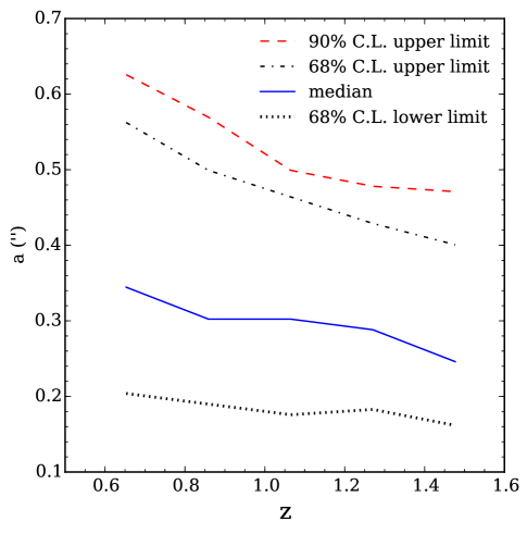
Figure 17: The 90% upper limit of the semi-major axis continuum size of H$\alpha$ galaxies with H$\alpha$ line flux $>10^{-16}\mathrm{erg/s/cm}^{2}$, $0.55<z<1.85$), based on 1773 galaxies from WISP (WISP team, private communication).

5.1.1.5 HLSS 5

Relative position measurement uncertainties shall be less than $3.4^{\prime\prime}$ over the entire survey area.

We need to measure galaxy positions to better than $\sim 0.1\mathrm{Mpc}/h$ (which corresponds to $3.4^{\prime\prime}$, assuming that 105 $\mathrm{Mpc/h}$ subtends 1 degree), in order to measure galaxy clustering accurately. This should be met easily if HLIS 26 is met, which makes systematic errors in the astrometry negligible. Given the pixel scale of $0.11^{\prime\prime}$, this requirement is automatically met within each field, and is tied to the precision of astrometry across different fields.

5.1.1.6 HLSS 6

The survey completeness shall be 50% (TBC), and the redshift purity shall be 90% (i.e., the outlier fraction is less than 10%). Completeness is defined as the fraction of H$\alpha$ ELGs with measured redshifts flagged as reliable, and purity is defined as the fraction of measured redshifts flagged as reliable that are actually within 2$\sigma$ of the true redshifts.

A requirement on completeness and purity is needed to translate the H$\alpha$ ELG number counts predicted by the H$\alpha$ LF to the galaxy number density that can be used to measure BAO/RSD by WFIRST GRS. The completeness of 50% and redshift purity of 90% are put in as crude estimates based on extrapolations from Euclid. Since WFIRST has a higher spatial and spectral resolution compared to Euclid, and more rolls (4 versus 3) per field, we expect a higher completeness and purity for WFIRST. The actual requirements will need to be validated by grism simulations, since these are determined by what are feasible given the instrumentation and the true universe. The requirement on the knowledge on the contamination fraction is set by HLSS 4.

5.1.2 Implementation Requirements (Level 2b)

In this section, we present the implementation requirements as delivered to the Project Office.

5.1.2.1 HLSS 7

The observatory shall provide a slitless spectroscopy mode, with a spectral dispersion no larger than 10.85 $\AA$/pix.

Gratings tend to give constant dispersion in linear space, rather than R-space. The above dispersion would give point-source spectral resolution $R=\lambda/\Delta\lambda$ in the range $550<R<800$, for a 2-pixel resolution element.

The grism resolution requirement is set by requiring the redshift precision to be 0.1% (set by BAO/RSD science), thus is not sensitive to which ELGs (H$\alpha$ vs [OIII]) we use as tracers. Going to lower spectral resolution would degrade the redshift precision and put BAO/RSD science goals at risk. The number density of [OIII] ELGs may be significantly higher than previously assumed; this gives some margin in the spectral resolution requirement due to the smaller sizes and less line blending of [OIII] ELGs.

Given the margin from a likely higher [OIII] ELG number density than previously assumed, we have removed the requirement on resolving H$\alpha$ and NII for all galaxies of radius $0.3^{\prime\prime}$, and 90% of galaxies of radius $0.54^{\prime\prime}$, which would drive the grism resolution higher. The blending of H$\alpha$ (6563$\AA$) and NII (6584$\AA$) leads to a metallicity-dependent shift in line centroid for larger sources; this would lead to a systematic bias in the measured redshifts, which can propagate into the BAO/RSD measurements. Having a higher grism resolution would alleviate this problem, at the cost of a reduction in survey depth, and more overlapping of spectra for galaxies. This is a trade study that we will carry out as the required grism simulations become available.

5.1.2.2 HLSS 8

Spectra shall achieve $S/N\geq 5$ for $r_{\mathrm{eff}}=300\mathrm{mas}$ for an emission line flux $~{}1.0\times 10^{-16}\ \mathrm{erg/cm}^{2}\mathrm{/s}$, from a source at 1.8 $\mu$m.

This sensitivity is sufficient to meet the comoving space density requirement HLSS 2 with some margin given best estimates of the H$\alpha$ luminosity function (Pozzetti et al., 2016) at these redshifts. The use of a $\mathrm{S/N}\geq 5$ threshold for an arbitrary spectrum pre-spectral-decontamination gives margin for detection of sources whose spectra overlap others, or for loss of some exposures to cosmic ray hits or other artifacts, as $\mathrm{S/N}\geq 5$ post-decontamination is expected to be sufficient for meeting the redshift accuracy requirement HLSS 4, and the post-decontamination S/N should be significantly higher than the pre-decontamination S/N for a given spectrum. Current calculations of observatory performance indicate that the sensitivity specified here is achieved in a total exposure time of $\sim 1200$ seconds per field.

The median continuum size (semi-major axis) of H$\alpha$ ELGs is $0.3^{\prime\prime}$ (see Figure 17). This sensitivity requirement is phrased in parallel with the sensitivity requirement of the WL survey. This depth is a factor of two to three deeper than the Euclid GRS. The depth is sufficient to give the required galaxy number density in HLSS 2.

5.1.2.3 HLSS 9

The uncertainty of the wavelength measurement $\lambda$ shall satisfy $\Delta\lambda/\lambda\leq 0.001$.

Although this is redundant since it is essentially the same as HLSS 4, it is necessary to keep it since it flows HLSS 4 into a dataset requirement.

5.1.2.4 HLSS 10

The spectroscopic bandpass shall satify $\lambda_{\mathrm{max}}\geq 1.9\ \mathrm{\mu m}$, and $\lambda_{\mathrm{max}}/\lambda_{\mathrm{min}}>1.82$.

We need $\lambda_{\mathrm{max}}>1.9\ \mathrm{\mu m}$ for redshift reach, in order to be complementary to Euclid and ground-based surveys. Furthermore, we need $\lambda_{\mathrm{max}}/\lambda_{\mathrm{min}}>1.82$ for line identification using multiple lines: to ensure that we cannot have [OII] (373nm) falling off the blue end of our coverage while H$\alpha$ (656.28nm) falls off the red end. We have assumed that the actual bandpass extends 1.5% from either end, since it is problematic to use emission lines that fall within 1.5% of the bandpass edges.

5.1.2.5 HLSS 11

50% of the energy (excluding diffraction spikes and non-1st order light) shall be enclosed in a circle of radius $<0.21^{\prime\prime}$ over 95% of the field.

This limit of $0.21^{\prime\prime}$ is required by source separation in the input catalog for spectral extraction, and is enabled by the addition of the phase mask corrector, and leaves some margin on the wavefront error.

5.1.2.6 HLSS 12

The filter used to define the bandpass of the grism shall have cutoff transition widths $\sigma<1\%$ (0.7% goal) after including the effects of broadening by the range of incident ray angles at each position in the FoV, where $\sigma$ is defined by $\sigma=(\lambda(T=0.90)-\lambda(T=0.10))/\lambda(T=0.50)$. $T$ is the transmission of the grism bandpass.

This is based on the grism guiding considerations; the assessment of grism guiding (and its positive outcome) assumed $\sigma<1\%$.

5.1.3 Implementation (Operations Concept) Requirements

We present here the implementation requirements related to the operation concept. We note that Co-I Hirata is the co-lead for the WFIRST Operations Working Group. We did not update Requirements HLSS 13-15, but include them here for completeness.

5.1.3.1 HLSS 13

Exposures of each field shall be obtained at a minimum of 3 dispersion directions, with two being nearly opposed.

5.1.3.2 HLSS 14

The observatory shall be able to place the WFC at a commanded orientation with an accuracy of $0.64^{\prime\prime}$ ($3\sigma$) in pitch and yaw, and $87^{\prime\prime}$ ($3\sigma$) in roll (TBR these were arbitrary values that give a net $3\sigma$ position uncertainty of 10 pixels. For the HLSS, the primary driver is that the position uncertainty is small with respect to chip gaps, which gives larger uncertainties than specified above. The smaller values quoted here are consistent with efficient target acquisitions, which would flow down from an observing efficiency spec.)

5.1.3.3 HLSS 15

The observatory pointing jitter and drift shall not exceed 100 mas in the spectral direction on the WFC focal plane (goal of 60 mas) and 50 mas in the cross- dispersion direction (TBR).

5.1.3.4 HLSS 16

Imaging observations shall be obtained of the fields in the HLSS that reach JAB=24.0, HAB=23.5, and F184AB=23.1 for an $r_{\mathrm{eff}}=0.3^{\prime\prime}$ source at 10$\sigma$ to achieve a reference image position, in 3 filters.

Provided the HLSS covers area already observed in the HLIS, this requirement will be met automatically. This requirement applies to any HLSS fields that are counted toward the minimum survey area requirement but are not covered by the HLIS. Imaging in at least three filters is required to build a minimal spectral template for grism spectral decontamination.

5.1.3.5 HLSS 17

There shall be 40 observations of two deep fields, each 11 deg² in area, sufficient to characterize the completeness and purity of the overall galaxy redshift sample. The 40 observations repeat the HLSS observing sequence of 4 exposures 10 times, with each deep field observation having the same exposure time as a wide field observation of the HLSS. The dispersion directions of the 40 observations should be roughly evenly distributed between 0 and 360 degrees.

To calibrate the HLS GRS, we need a spectroscopic subsample, with the same selection criteria as that of the HLS GRS, containing more than 160,000 galaxies that have a redshift purity $>99\%$. We need 160,000 galaxies to know the redshift purity to 1% (which requires 10,000 objects, assuming noise of $1/\sqrt{2N}$ from Poisson statistics) in at least four categories (low z, high z, faint, luminous).

Based on the estimated galaxy number density of $>7273$ per deg² at the flux limit for the GRS, $10^{-16}\mathrm{erg}\,\mathrm{s}^{-1}\mathrm{cm}^{-2}$, we need a total area for the deep fields of 160,000/7273=22 deg². These can be split into two subfields of 11 deg² each. Smaller subfields prevent the testing of galaxy clustering statistics in each subfield. Each deep field should be part of the HLS footprint, so they are representative of the GRS as a whole.

The visits to the deep field should consist of 10 sets of HLS-GRS-like visits, matching the integration time, dither pattern, and observational time-sequence of the HLS-GRS strategy, with each set of HLS-GRS-like visits covering the same areas of 22 deg². Assuming a completeness of 50% and uncorrelated sets, the completeness after 10 sets of visits is (1-0.5)10=0.001, leading to a 99.9% complete sample for calibrating the GRS. Since each set of observation consists of 4 roll angles, the total number of deep field observations is 40. The dispersion directions of the 40 visits should be roughly evenly distributed between 0 and 360 degrees, in order to map out possible sources of systematic errors due to inhomogeneity.

5.1.3.6 HLSS 18

The observing efficiency of the HLSS, defined as the total science exposure time divided by the total time allocated to the survey, shall be TBD%.

The total time includes slew, settle, target acquisition, and calibration observations that are specific to the HLSS, including the extra-depth observations of the deep fields described in HLSS 17. This minimum observing efficiency, together with a 0.67 year total allocation of observing time, allows science exposures of 1600 deg² (TBC) with the exposure time indicated in the comment to HLSS 8; this provides a 7% (TBC) margin over the 1500 deg² requirement (HLSS 1) to allow for data that may be unusable because of instrumental artifacts, bright sky objects, etc. This is a high level requirement that will need to be revisited as the mission implementation details become more solid; it should be set such that the core science goals for the GRS are achieved without putting mission success at risk.

5.1.4 Calibration Requirements

In this section, we present the calibration requirements as delivered to the Project Office.

5.1.4.1 HLSS 19

The relative spectrophotometric flux calibration shall be known to 2 percent relative accuracy (with the goal of 1%), in order to understand the effective sensitivity limit for each redshift bin for each area surveyed.

The requirement here is only on the relative spectrophotometry, which impacts the selection function of galaxies. Absolute line flux calibration will only change the overall number of objects and the dN/dz, but will not introduce density variations. Large scale structure measurements require precise knowledge of the selection function of galaxies. Although the overall redshift distribution may be determined by averaging over the entire survey, fluctuations in the selection function can easily contaminate the underlying cosmological density fluctuations.

The spectroscopic sample for the GRS is expected to be defined by a line flux limit of 10${}^{-16}\,$erg s^-1cm^-2. Spatial errors in the spectrophotometric calibration will introduce artificial spatial fluctuations in the number density of galaxies, which could contaminate the cosmological signal.

We start by setting a requirement on the spatial uniformity of the mean number density as a function of physical scale. We require that the non-cosmological fluctuations in the mean number density (or the selection function of the survey) be $<1\%$ (sqrt variance) when averaged over spatial scales between 10 Mpc/$h$ to 200 Mpc/$h$. At small scales, this is $\sim$ two orders of magnitude smaller than the cosmological signal, while at the $\sim$ BAO scale of 100 Mpc/$h$, this is $\sim$ one order of magnitude smaller than the cosmological signal. These fluctuations equal the cosmological signal at $\sim 400\mathrm{Mpc}/h$. These physical scales correspond to $\sim 0.5$ degrees to 6 degrees at a redshift of 1.5.

We convert the above requirement to a requirement on the spectrophotometric calibration accuracy, assuming the Model I luminosity function of Pozzetti et al. (2016). At the flux limit of WFIRST, this yields a requirement of 1% relative spectrophotometric calibration, averaged over angular scales of 0.5 degrees to 6 degrees.

This is a very stringent requirement. We have relaxed this requirement from 1% to 2% to add margin for mission success, assuming that we will achieve 1% relative spectrophotometric flux calibration in post-processing by projecting out problematic modes in the analysis.

We plan to make this requirement more precise, in the form of “The relative spectrophotometric flux shall be known to 2% relative accuracy in TBD (probably the spectral resolution) wavelength bins with a goal of 1% on scales larger than TBD (per pointing, 0.3 deg) and TBD% on scales smaller than 0.3 deg.” We are working on deriving and justifying these numbers. Co-I’s Capak, Hirata, and Padmanabhan are members of the WFIRST Calibration Working Group, working on a detailed calibration strategy for WFIRST.

5.1.4.2 HLSS 20

The uncertainty in the wavelength calibration shall not introduce biases in the wavelength measurement by amounts greater than $\Delta\lambda/\lambda=10^{-4}$ on any angular scales exceeding 0.064 degrees within a field, and $\Delta\lambda/\lambda=2\times 10^{-5}$ from field to field.

Variations in the wavelength calibration within a field, and from field to field on large scales, wash out the clustering signal by de-correlating the projected component of the clustering signal on those angular scales.

Within a field, the acceptable level of wavelength error is $\Delta\lambda/\lambda\sim 10^{-4}$, which is 10% of the errors on individual redshift measurements (0.001), to avoid increasing the overall redshift error by a significant factor. The angular scale is set by the optimal smoothing scale for BAO reconstruction, $\sim 5\,\mathrm{Mpc}/h$. At $z=3$, this subtends 0.064 degrees for a flat universe with $\Omega_{\mathrm{m}}=0.3$ and a cosmological constant.

For field to field, the acceptable level of wavelength error is $2\times 10^{-5}$, which comes from comparing two adjacent fields. Since we expect $\sim 10^{4}$ galaxies per deg², we have $\sim 2810$ galaxies per FOV of 0.281 deg². If the galaxies have a redshift error of $10^{-3}$ each, then one can measure systematic offsets between fields (statistically) at the $10^{-3}/\sqrt{2810}$ level, which is $1.9\times 10^{-5}$. At that level the power from the systematics is sub-dominant to the power from the redshift error.

5.1.5 Requirements on Science Data Products:

In this section, we present the GRS requirements on science data products. We are in the process of studying HLSS 21-25. These depend on the structure and responsibilities of the SOCs and the SITs. Co-Is Teplitz and Capak have extensive experience in data processing for space missions, and have provided detailed comments on these requirements to the WFIRST Project Office.

5.1.5.1 HLSS 21

The raw data for each grism exposure shall be available through the archive, with each dataset including identifying information such as time of exposure, observatory pointing orientation, a unique dataset identifier, and any engineering information needed for subsequent processing. Each detector readout for a given exposure shall be included in the dataset.

5.1.5.2 HLSS 22

Calibrated data for each grism exposure shall be available through the archive. Each detector readout shall be calibrated at the appropriate level, and the individual calibrated readouts will be combined to produce a net spectral image. These datasets shall include information on the effective PSF as a function of position and incorporate any World Coordinate System information needed for subsequent stages of processing. As sources are not yet identified, association of a pixel with a source position and wavelength is not yet possible.

5.1.5.3 HLSS 23

Source catalogs of the same field derived from WFC imaging data shall be combined with observatory pointing information for each grism exposure to produce a segmentation map that associates each catalog source with a range of spectral image pixels. The spectral images of bright stars in each detector shall be used to refine the astrometric solution. These segmentation maps shall be used to extract 1D spectra for each source, and to flag pixels that may contain flux from multiple sources. The extracted spectra shall include information on the effective exposure time for each pixel, effective PSF as a function of position, data quality flags, and any other information needed to interpret the data.

5.1.5.4 HLSS 24

Extracted spectra of each source from multiple roll angles shall be combined to produce a single net spectrum of each source. For sources that are spatially resolved, the result shall be provided as a data cube of position and wavelength. The spectra obtained at nearly opposing roll angles shall be used to account for possible offsets of the emitting region from the center of the broad-band image. The data from all roll angles shall be used, to the extent possible, to resolve ambiguities in the proper source to associate with pixels illuminated by overlapping spectra. These net spectra shall include information on the effective exposure time for each pixel, statistical and systematic uncertainties in the measured fluxes and wavelengths, effective PSF as a function of position, data quality flags, and any other information needed to interpret the data.

5.1.5.5 HLSS 25

The data processing system shall have the capability of inserting fake sources into the spectral image data and re-executing the generation of high-level science products. These tests are essential for verifying the proper operation of the tools that generate high level science products and for understanding the sensitivity of the survey and systematic effects that may be present in the survey sample.

5.1.5.6 HLSS 26

The data processing system shall provide sufficient knowledge of the 3D selection function so that the artificial correlations due to inaccuracies in the 3D selection function are less than 10% of the statistical error bars on scales smaller than 2 degrees, and less than 20% on larger angular scales.

This requirement is only meaningful in terms of the contribution to the total error budget by the uncertainties in the 3D selection function. The BAO scale is less than 2 degrees in the redshift range for the HLSS.

To convert the positions of observed galaxies in the large-scale structure into clustering measurements (correlation function, power spectrum, higher order statistics) we need to know how the “average” number density of objects (in the absence of clustering) changes in the observed volume. The mean number density will vary significantly both in redshift and with angular position due to effects of target selection, data reduction and observing conditions. Previous surveys were able to separate the selection function in two independent parts: the radial selection function and the angular selection function. It is likely that the WFIRST selection function will not be separable in this way, i.e. different parts of the sky will have different radial profiles. For now we will assume that this type of separation is possible. This assumption is reasonable for preliminary investigation since most effects are either mostly radial (e.g. target selection, data reduction) or angular (e.g. imaging quality, galactic extinction).

The knowledge about 3D selection function is usually encoded into sets of random catalogues. When computing clustering statistics, the random catalogues remove the systematic effects of varying mean number density (due to target selection, data reduction or observing conditions). If the 3D selection function is not correct, the effects will not be completely removed and will generate spurious correlations that can bias the true cosmological signal. The angular mask of the WFIRST data will vary pixel to pixel on the infrared detector. The full description of the angular mask may turn out to be computationally intractable. For the core science goals we require the description of the mask to be correct with an angular resolution of approximately 3 arcmin. This corresponds to a spatial resolution of $3\,h^{-1}\mathrm{Mpc}$ at $z=1.5$. This is driven by the fact that we need to be able to resolve the BAO peak. In principle, our requirements on the knowledge of the 3D selection function are driven by the main requirement that the spurious correlations should be no more than TBD per cent of statistical errors between the scales of 10 and 150 h^-1Mpc in clustering signals (either in correlation function multipoles or power-­spectrum). For the galaxy sample expected from WFIRST, this corresponds to TBD per cent uncertainty in the knowledge of the radial distribution and the angular mask.

To further quantify the effect of systematics offset in the angular mask on clustering measurements we have performed tests on mock catalogues representing BOSS CMASS sample. This is justified by the fact that the BAO and growth rate measurements from WFIRST GRS in redshift bins of $z\sim 0.1$ are expected to be roughly equal to the CMASS constraints with $z\sim 0.2$.

The mock surveys are generated from N-body simulations, with a median redshift of 0.6, with galaxies of halo mass range about $7\times 10^{13}\,M_{\odot}$. The mock surveys have proper BOSS 3D selection function (which we take as truth here). Now we distort the selection function in the following scenarios:

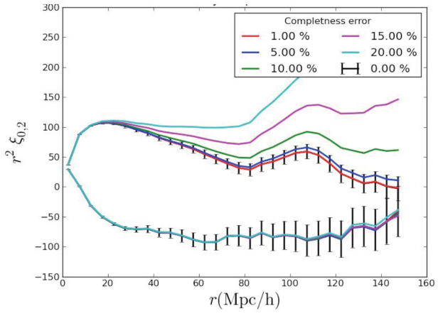
Figure 18: The monopole (upper curves) and quadrupole (lower curves) of a single mock survey and how they respond to various completeness errors in the scenario described in scenario. We can see from the level of two point correlation function, even a 5% error on the completeness can change the monopole and quadrupole significantly that we expect RSD to be affected, while BAO is not significantly affected, as this mostly changes the amplitude of the correlation function.

1. The survey region is divided into two equal area along RA and one area has true completeness whereas the other one has $1-x$ completeness where x is a given completeness error (as shown in the legend of Figure 18). We show in Figure 18 the resulting monopole and quadrupole with varying completeness error. This is an interesting limiting case as surveys can sometimes be affected by large scale systematics generated by either calibration of two parts of the sky, or due to large scale effects caused by the galactic foregrounds.

2. The true survey completeness is multiplied with a gaussian function. The gaussian function has mean 0 and variance as the denoted completeness error. We then fold both positive and negative side of the Gaussian to the negative side and hence allow the completeness to be only smaller than its true value. We vary the scale at which we change the 3D selection function, starting with 1 degree to 4 degrees (4 deg. is approximately the BAO scale at this redshift).

From the preliminary analysis shown here, we expect that we will need to accurately model the 3D completeness function down to a few % level. At 5% the effects can already be very detrimental to our large scale structure analyses using BAO and RSD. Scaling from these, we arrive at the requirement that artificial correlations due to inaccuracies in the 3D selection function are less than 10% of the statistical error bars on scales smaller than 2 degrees, and less than 20% on larger angular scales.

5.1.6 Requirement on Cosmological Volume Simulations:

We now present a new category of requirements for a space mission. These are not needed for mission success (data acquisition by the spacecraft), but only for meeting the high level science requirements (level 1). We summarize these as follows:

1. a few accurate mocks with galaxies included using semi-analytical galaxy formation model, to verify and validate WFIRST GRS pipeline;

2. $\sim 100$ mocks with high mass resolution of 109 solar masses, to inform theoretical modeling of the data;

3. $\sim 10,000$ mocks with low resolution, to derive the covariance matrices for the WFIRST data.

To quantify the requirement on cosmological volume simulations, we consider only the case for galaxy clustering science (which includes BAO and RSD) for now for simplicity. For WFIRST, simulations are required for the following three objectives:

1. establishing the basic correctness of the pipeline;

2. informing the theoretical modeling of small scale clustering as a function of tracer properties;

3. calculating the covariance matrix for each GRS probe and across many probes.

In order to establish the basic correctness of the WFIRST pipelines and predictions, sophisticated synthetic mock galaxy catalogs are essential. These catalogs, which must realistically emulate WFIRST both in sky area and depth, are typically constructed by running large gravity-only simulations and then “painting” realistic galaxies on top. Populating a simulation with galaxies can be done in several ways: (i) empirically, using statistics such as the “halo occupation distribution”, (ii) by placing the normal, baryonic matter in the simulation ab initio and explicitly solving the hydro-dynamical equations, or (iii) by using a semi-analytical galaxy formation model (SAM), whereby the astrophysical processes and formation histories of galaxies are described using physically motivated, parameterized equations. The advantage of SAMs over alternative methods is their ability to meet the demands from next generation cosmological surveys for large (suites of) galaxy mock catalogues that are both accurate and can be constructed rapidly. In contrast, full hydro-dynamical simulations are far too slow and empirical methods are limited by the availability of existing high redshift observations, which are necessary for the calibration of these methods. SAMs also require some observations for calibration but, once tuned to fit observations at low redshift, they are able to make predictions out to high redshift without the need for further observational input. Furthermore, empirical methods are often limited in that they are calibrated in one or two photometric bands, whilst SAMs are designed to model the star formation history of a galaxy and so have the ability to make predictions for a wide variety of multi-wavelength data simultaneously. This feature of SAMs is vital to ensure that we can examine cross-correlations between the spectroscopically-selected dataset for galaxy clustering analysis and the photometrically-selected dataset for weak lensing analysis. Besides testing the pipeline and making (limited) cosmological forecasts, these galaxy mock catalogs would also be a valuable resource for science working groups focusing on legacy science (e.g. galaxy evolution, active galactic nuclei). Note that, compared to the large number of approximate mock catalogs necessary for covariance estimation, only very few accurate galaxy mocks are required to verify and validate the WFIRST pipeline.

To inform the theoretical modeling of clustering especially at non-linear scales as a function of the tracer properties would require a significant number of simulations that have relatively realistic modeling of the tracer properties at the relevant redshift. For WFIRST, we can take the current number density of emission line galaxies (for H$\alpha$ galaxies only) from our baseline calculation and used the Tinker et al. (2008) halo mass function, along with the Giocoli et al. (2008) subhalo mass functions to compute the total number of halos and subhalos above some mass threshold and then match that to the baseline GRS number densities. This maps back to approximately 10${}^{1}2$ solar masses from z=1 to z=2. Assuming that we need to have at least 100 particles to resolve halos at 1012 solar masses, and another factor of 10 particles to resolve properties of the halo progenitors, we will need dark matter particle mass resolution of approximately 10⁹ solar masses. The extra factor of 10 is due to the galaxy formation model that depends on the properties of the progenitors which is an approximation that may change as we understand the galaxy properties better and as more observations of the tracers arrive. We expect to require of order 100 simulations to reduce the shot noise of the correlation function in order to compare the theoretical modeling to the simulated correlation function. These realistic mock surveys may also require the modeling of non-standard cosmological models, such as extensions to non-zero total neutrino masses, or modified gravity models.

Finally, we will need to calculate the covariance matrices of the main probes of clustering, namely BAO and RSD, and the cross-covariances among these probes (or across different methods as in recent BOSS analyses). We can approach the calculation of the covariance matrices through multiple avenues. One can generate (in principle) a large number of approximate mock surveys using relatively fast approximate methods (eg., PTHalos, QPM, FastPM, etc), and apply the relevant survey properties onto these mock surveys. The small scale modeling of the clustering may not be 100% accurate, but is likely to be adequate for the linear RSD modeling and BAO analyses where medium to large scales are most important. The number of approximate simulations required can be on the order of O(10,000) depending on the number of parameters we will be estimating using these covariance matrices, but the time requirement of these approximate mocks is relatively modest. One can also envision using more theoretical approaches (such as O’Connell et al. (2016); Padmanabhan et al. (2016); Friedrich et al. (2016), which only require a relatively modest number of realistic mock surveys which are required for (b).

5.2 GRS Light-cone Simulations (D8, D9)

Light-cone cosmological simulations are a critical tool to design the GRS survey design, to develop and to validate analysis tools and theoretical predictions. We developed four complementary simulation approaches to tackle multiple questions relevant to the GRS:

1. A lognormal simulation to generate quickly large cosmological volumes;

2. A fast approach using simple galaxy-halo prescriptions to generate joint GRS and WL simulations;

3. A realistic emission line galaxies modeling to study the confusion between H$\beta$ and [O III] emitters;

4. A realistic semi-analytic galaxy evolution model to make robust H$\alpha$ mock catalogs.

In order for WFIRST HLS to reach its high level science requirements, we have proposed to (D9) produce simulated light-cone observations to (D8) develop both the methods for modeling and interpretation of cosmological measurements from WFIRST. Most of these data sets will be at the level of galaxy redshift and shape catalogs rather than the pixel-level imaging and spectroscopy simulations described above. They will incorporate varying degrees of complexity regarding galaxy bias, redshift evolution, survey geometry, and observational systematics such as incompleteness, shape measurement errors, and photometric redshift biases. Many of these artificial data sets will be made publicly available, and some will take the form of data challenges, where the underlying parameters are initially known only to the creators of the data set. Here we report on our first year simulation efforts in a 4 prong approach, ranging from the largest volume to the highest resolution below:

5.2.1 Lognormal Simulations

Samushia and his postdoc have produced a suit of few thousand fast “enhanced log-normal simulations” for the WFIRST GRS expected samples. While these simulations do not correctly reproduce the small scale structure and higher order statistics of the field, they can be used for studying various large scale effects and implement light-cone effects. The simulations have so far been used to study the effect of splitting the WFIRST footprint into two non-contiguous areas. We plan to use these simulations in the future to study systematic effects in the measurements (e.g., window effect correction) and to validate the BAO/RSD proto-pipeline. These simulations are very well-suited for such tasks since their input two-point signal is known exactly.

5.2.2 Fast simulations with galaxy positions and shapes

Kiessling, and Huff are working with Postdoc Izard to develop a fast pipeline to provide galaxy mock catalogues with weak lensing. The goal of our initial project is to model effects of various systematics and determine their impact on galaxy clustering and weak lensing observables and their covariance matrices. The starting point for this project is 300 ICE-COLA fast simulations (Tassev et al., 2013; Izard et al., 2016) generated by Izard during his PhD that provide the dark matter density field and halo catalogs (both in the light cone geometry). The former is used to compute maps of weak lensing distortions in the Born approximation using a technique developed by Izard (Izard et al, 2017; in prep). Galaxies are attached to halos using a new pipeline developed for this project. This pipeline takes the halo catalogues in the light cone geometry generated by the fast simulations and produces galaxy samples with broad band luminosities and weak lensing properties. The produced catalogs are all sky and span 0 $<$ z $<$ 1.4, with a minimum dark matter halo mass of $10^{12}M_{sun}/h$.

5.2.3 Testing the effect of line confusions on BAO using N-body simulations

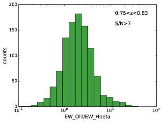
Figure 19: The line ratios between H$\beta$ and [O III] using the dataset from DEEP2 survey, which has acquired over 50,000 emission line galaxies, but a significant fraction of them have H$\beta$ and/or [O III]. The plot shows $\approx$1,000 galaxies from DEEP2 sample that has both H$\beta$ and [O III], while each line is detected at least at 7-$\sigma$.

Ho and Massara concentrates on one particular goal in generating their simulations. Their goal is to investigate the effect of confusion between H$\beta$ and [O III] emitters, in particular in the high level science goal in BAO. In WFIRST, the primary science targets for the redshift survey will be H$\alpha$ and [O III]. There is a special concern of H$\beta$ vs. [O III] confusion due to their proximity in wavelength (hence the inability of photo-z’s to distinguish them reliably). This is particularly true given that an H$\beta$ emitter mis-identified as [O III] will have an inferred radial position different by 8900 km/s (or: 89 $h^{-1}Mpc$ * (1+z)/$\sqrt{\Omega_{\Lambda}+\Omega_{m}(1+z)^{3}}$, which in our range of redshifts is near the BAO scale). We will also get some [O II] emitters – these might be useful directly for cosmology, or for disentangling other line emitters (see Pullen et al. 2014). Note that at WFIRST resolution 3726 and 2729 are a blend.

A key challenge in the mocks will be making sure the populations of each line and the correlations among the different line strengths and with environment are sufficiently realistic for the tests we are doing. This has historically proven to be very difficult due to the heterogeneous nature of the observational constraints. Therefore, we have investigated the equivalent width ratio between H$\beta$ and [O III] using the dataset from DEEP2, which has acquired over 50,000 emission line galaxies, but a significant fraction of them have H$\beta$ and/or [O III]. This is so far one of the few statistical samples that can be used to look at the line ratios (see Figure 19). We also look at the conditional luminosity function between the two line luminosity observed in DEEP2 (see Figure 20). We now proceed to use these line ratios to create the emission line galaxy catalog.

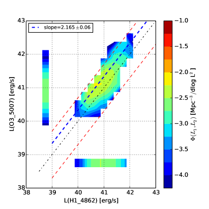
Figure 20: The conditional luminosity function between H$\beta$ and [O III] using the same galaxies as in Figure 19. The black and red lines are the conditional luminosity function (and 1 sigma) from DEEP2 survey).

We start with dark matter simulations generated by Stanford group (led by Risa Wechsler, which is part of WFIRST Simulation WG and belongs to the EXPO SIT) that contain galaxies up to 5-sigma detection limit of grizY = [27.5, 27.0, 26.4, 25.9, 24.0] over 10313 sq. degrees. Each of the galaxy contain its own spectral energy distribution which are generated to fit most updated luminosity function and color evolution measurement. Galaxy magnitudes and shapes are affected by shear and magnification. We then measured and validated the correlation function and luminosity function of [O III] selected galaxies (with WFIRST detection limits). Next, we plan to apply the measured line ratios as described in Figure 19 to all the galaxies and reapply the WFIRST detection limits to create a realistic WFIRST emission line galaxy catalog (with [O III] as the main galaxy targets), and assess the effects on BAO peak position due to the possible smearing by mis-identifying the H$\beta$ as [O III]. In addition to the mocks themselves, it will be important for us to identify which aspects of the emission lines we think are close to reality, which are of the right order of magnitude, and which could be qualitatively different from the real Universe. We envision that we would continue improving these up to the point where we have the real WFIRST data.

In addition, we have also released a code that calculates the interloper fraction (Wong, Pullen & Ho): a Python-based program that applies secondary line identification and photometric cuts to mock galaxy surveys, in order to simulate interloper identification. We also have a module specifically designed to do WFIRST and predict interloper rates for WFIRST (Wong et al., 2016).

Figure 21: The correlation function of [O III] galaxies with WFIRST detection limit within our 10,000 sq.deg simulations.

5.2.4 H$\alpha$ emitter number density forecasts

In work led by Merson, Wang, Benson, Masters, Kiessling and Rhodes the open source semi-analytical galaxy formation model, Galacticus (Benson, 2012), was used to predict the H${\rm\alpha}$-emitter number counts and redshift distributions for the WFIRST GRS. This work is published in Merson et al. (2018).

A four square degree lightcone catalogue was constructed by processing the dark matter merger trees of the Millennium Simulation (Springel et al., 2005) with the Galacticus model. Emission linesare modelled in Galacticus by interpolating over a library of emission line luminosities obtained from the Cloudy (Ferland et al., 2013) code and stored as a function of hydrogen (HI), helium (HeI) and and oxygen (OII) ionising luminosities, as well as the hydrogen gas density and metallicity of the interstellar medium (ISM). The emission line luminosities are then processed to incorporate attenuation due to interstellar dust, which can be modelled using several different methods. Merson and collaborators consider three dust methods from Ferrara et al. (1999), Charlot and Fall (2000) and Calzetti et al. (2000). However, it is worth noting that any user-specified dust method can be used in conjunction with Galacticus.

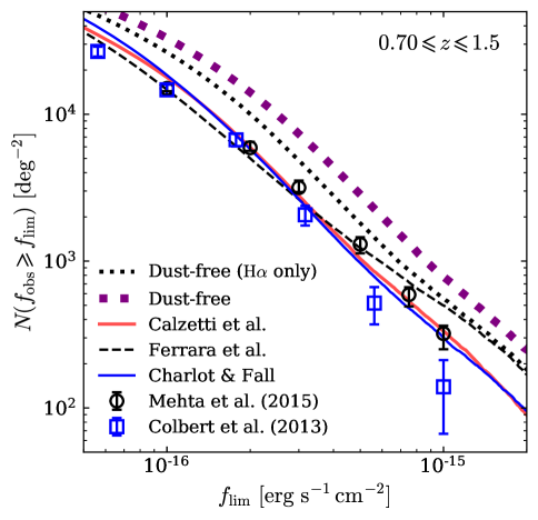
Figure 22: Predictions for the cumulative H${\rm\alpha}$ flux counts for the redshift range $0.7<z<1.5$ from a Galacticus lightcone mock catalogue. The dotted lines show the counts assuming dust-free fluxes. Apart from the thin dotted line, which shows the counts for the pure H${\rm\alpha}$ luminosities, all lines show counts corresponding to the ${\rm H\alpha}+{\rm N\left[II\right]}$ blended counts. When adopting one of the dust attenuation methods; Ferrara et al. (1999), Charlot and Fall (2000) or Calzetti et al. (2000); the dust parameters are optimized using a chi-squared minimization technique comparing the Galacticus to those of Mehta et al. (2015). Full details can be found in Merson et al. (2018). The open data points show the observed blended flux counts from Colbert et al. (2013) and Mehta et al. (2015).

First, the Galacticus predictions for the cumulative counts of H${\rm\alpha}$-emitting galaxies over the redshift range $0.7\leqslant z\leqslant 1.5$ obtained with each dust method are compared with the latest WISP counts from Mehta et al. (2015). The H${\rm\alpha}$ luminosities from Galacticus are corrected to introduce contamination due to N[II] by cross-matching the Galacticus with galaxies from the SDSS catalogue of Masters et al. (2016). For each Galacticus galaxy, the five nearest neighbour galaxies in stellar mass versus specific star-formation rate space are identified from the SDSS catalogue. The H${\rm\alpha}$ luminosity of the Galacticus galaxy is then corrected according to the median ${\rm N\left[II\right]}/{\rm H\alpha}$ ratio from these neighbors. Further modelling of the ${\rm N\left[II\right]}/{\rm H\alpha}$ ratio as a function of redshift and stellar mass is presented by Fai .

The blended ${\rm N\left[II\right]}+{\rm H\alpha}$ luminosites are then attenuated using each of the three dust methods in turn. A chi-squiared minization technique is used to identify the optimum dust parameters needed so that the number counts from Galacticus are consistent with the observed counts of Mehta et al. (2015) down to a flux limit of $1\times 10^{-16}{\rm erg}\,{\rm s}^{-1}{\rm cm}^{-2}$ (see Figure 22). The chi-squared values indicate that the counts obtained from the Calzetti et al. (2000) dust method lead to the best agreement with the observed counts from the WISP survey. By using the optimized dust parameters, Merson et al. (2018) find that down the expected flux limits of the WFIRST mission, the Galacticus model is able to predict number densities that are consistent with existing observations from the WISP survey. Although the lightcone used in this analysis has a small area on the sky, it is expected that cosmic variance has little effect on the predicted number counts. Since the lightcone analysis is time-consuming and expensive in computing resources, the lightcone used in this study was limited in size to 4 sq deg, in order to provide timely input to WFIRST. However, Merson, Wang and Benson plan to build significantly larger lightcones in future work.

After setting the strength of the dust attenuation for each method, Merson et al. (2018) then examine whether the optimized attenuation strengths yield reasonable matches to the observational estimates for the distribution of optical depths (at the observer-frame H${\rm\alpha}$ wavelength) and the H${\rm\alpha}$ line luminosity function. For each of the dust models, Galacticus predicts optical depths that are consistent within error with the optical depth estimates from WISP (Domínguez et al., 2013), though the Galacticus optical depths do not show any increase with observed H${\rm\alpha}$ luminosity, as has been suggested in the literature. The predicted luminosity function from Galacticus is consistent with the H${\rm\alpha}$ luminosity function from WISP as measured by Colbert et al. (2013) over the redshift range $0.9\leqslant z\leqslant 1.5$. Comparison with the luminosity functions from HiZELS (Sobral et al., 2013) at $z\simeq 0.84$, $z\simeq 1.47$ and $z\simeq 2.23$ shows that with these chosen dust attenuations Galacticus is able to reproduce the $z\simeq 0.84$ luminosity function, but becomes progressively a worse fit towards higher redshift, especially at $z>2$. This suggests that the dust methods may be lacking some redshift evolution or dependence on other galaxy properties, or that the Galacticus emission line luminosities are the incorrect strength. Investigating these possibilities requires rigorous calibration of the Galacticus model, which will be carried out in future work.

Table 2: Predicted cumulative number of H${\rm\alpha}$-emitting galaxies per square degree for the WFIRST GRS, assuming a redshift range of $1\leqslant z\leqslant 2$. The fluxes were attenuated by, for each dust method, Monte-Carlo sampling likelihoods for the dust parameters 1000 times for each galaxy. This table shows the mean and standard deviation from these 1000 realizations. Further details can be found in Merson et al. (2018). The upper half of the table shows the counts assuming blended ${\rm H\alpha}+{\rm N\left[II\right]}$ fluxes, whilst the lower half of the table shows the counts from de-blended ${\rm H\alpha}$ fluxes. Predicted counts are reported for three dust methods: Calzetti et al. (2000), Charlot and Fall (2000) and Ferrara et al. (1999). Note that the flux limits correspond to blended ${\rm H\alpha}+{\rm N\left[II\right]}$ fluxes. The efficiency of the survey is instrumentation dependent, and has not been included.

Flux limit	Dust method used with Galacticus
${\rm erg}\,{\rm s}^{-1}{\rm cm}^{-2}$	Ferrara et al. (1999)	Calzetti et al. (2000)	Charlot and Fall (2000)
Cumulative counts for blended ${\rm H\alpha}+{\rm N\left[II\right]}$ fluxes
$1\times 10^{-16}$	$10403\pm 138$	$15176\pm 528$	$12195\pm 987$
$2\times 10^{-16}$	$3797\pm 60$	$4307\pm 170$	$3059\pm 230$
$3\times 10^{-16}$	$2263\pm 33$	$2084\pm 73$	$1414\pm 75$
Cumulative counts for ${\rm H\alpha}$ de-blended fluxes
$1\times 10^{-16}$	$7467\pm 102$	$10566\pm 402$	$8365\pm 765$
$2\times 10^{-16}$	$2827\pm 42$	$2877\pm 108$	$2025\pm 140$
$3\times 10^{-16}$	$1771\pm 24$	$1479\pm 46$	$1032\pm 45$

Finally, the Galacticus lightcone is used to present predictions for the redshift distribution and the differential and cumulative blended ${\rm H\alpha}+{\rm N\left[II\right]}$ flux counts for the WFIRST GRS, as well as two surveys mimicking a Euclid-like selection. Dust attenuation is applied by converting the results from the chi-squared minimization into a dust parameter likelihood. For each dust method the flux counts are estimated 1000 times by Monte-Carlo sampling from these likelihoods. Merson et al. (2018) find that for a WFIRST GRS with redshift range $1\leqslant z\leqslant 2$ and blended flux limit of $1\times 10^{-16}{\rm erg}\,{\rm s}^{-1}{\rm cm}^{-2}$, Galacticus predicts a number density between 10,000 and 15,000 galaxies per square degree. Number counts for the three dust methods are shown in Table 2. The predicted cumulative flux counts are compared to forecasts from empirical models originally presented by Pozzetti et al. (2016). At at flux limit of $1\times 10^{-16}{\rm erg}\,{\rm s}^{-1}{\rm cm}^{-2}$, comparable to the flux limit of the WFIRST GRS, the Galacticus counts from the three dust methods are in closer agreement with each other than the counts from the three Pozzetti et al. (2016) models. Merson et al. (2018) find that these faint fluxes the Galacticus counts are most consistent with Pozzetti et al. (2016) model three, which of the three empirical models gives the lowest counts for faint fluxes. At brighter fluxes, approaching $1\times 10^{-15}{\rm erg}\,{\rm s}^{-1}{\rm cm}^{-2}$, the Galacticus counts show closer agreement with Pozzetti et al. (2016) model two, which predicts the highest counts for bright fluxes. Note that all the H${\rm\alpha}$-emitter counts discussed in Merson et al. (2018) are expected number counts of target galaxies for spectroscopy, and not the counts of galaxies with redshift measurements. The latter will depend on the redshift purity and completeness for each survey, which in turn depends on instrumentation and noise parameters. In this section, we have illustrated that our multiple simulation efforts complement each other in different ways. LogNormal and Fast simulations with both positions and shapes, are useful for pipeline testing and constructing covariance matrices. The more realistic simulations will test various assumption and requirements we make for WFIRST HLS. For example, do we need higher resolution in the grism to disentangle the [O III] and H$\beta$? Do any of these line ratios or galaxy properties depend on environment? Would it lead to an environment dependent BAO smearing if we do not take these into account? As we develop more realistic galaxy simulations such as those with Galacticus, we will be able to use the appropriate prescription for galaxy properties we cannot measure with current observations and make our final WFIRST simulation as realistic and physically driven as possible. We will examine a variety of other properties of emission line galaxies, including the distribution of OIII luminosities fluxes and the contamination from NII. This will allow us to have the best tool to develop both the methods for modeling and interpretation of cosmological measurements from WFIRST, and release the most realistic WFIRST galaxy catalog to the public before WFIRST launch.

5.3 Improving our Knowledge of the H$\alpha$ Luminosity Function

Knowing the H$\alpha$ and [OIII] luminosity functions is critical in order to optimize the WFIRST GRS. We are addressing current limitations in our knowledge using a newly available set of HST spectroscopic data within the WISP collaboration.

In order to trace the galaxy distribution through z$\sim$2.7, the future WFIRST surveys will make use of H$\alpha$ and [OIII] selected emission line galaxies. These two lines will allow WFIRST to cover the redshift range 1$<$z$<$2 (H$\alpha$) and 2$<$z$<$2.7 ([OIII]) respectively. Therefore, knowing the expected number of H$\alpha$ galaxies in the survey volume is required and the study of the H$\alpha$ luminosity function (LF) become fundamental in order to optimize the planned redshift surveys. However, despite the numerous works on this topic, given the high uncertainties associated to the H$\alpha$ LF determination, a sufficiently precise measure is still lacking (Figure 23). Additionally, the samples of emission-line galaxy are expected to be affected by a complex selection function that depends on galaxy luminosity, size, line equivalent width and also on contamination from mis-identified single emission-line galaxies at different depths.

A newly available set of HST spectroscopic data, gathered in the context of the WFC3 Infrared Spectroscopic Parallel (WISP) survey (Atek et al., 2010), of which team members Teplitz and Baronchelli are members, has recently become publicly available. Currently, this survey covers a total area of more than $\simeq$ 2000 sq. arcmin., with thousands of emission lines from a total of $\sim$500 randomly distributed HST pointings identified between z=0.3 and z=1.5. Thousands of emission lines from a total of $\sim$500 randomly distributed HST pointings have already been identified by the WISP team, between z=0.3 and z=1.5. The spectroscopic capabilities of HST+WFC3 are comparable to those that WFIRST can reach over a 2-order of magnitude wider area. This fact makes the WISP survey a particularly suitable test bench to optimize the future WFIRST surveys.

The accurate constraint of the parameters defining the line LF ($\phi^{*}*,L^{*},\alpha$) is hindered by their high correlation. Therefore, estimating these parameters requires uniform sampling of both the bright and faint ends of the luminosity distribution. In the next months, in the context of a collaboration involving both WISP and SIT members, Teplitz, Baronchelli and Wang, are planning to obtain the most accurate estimate, to-date, of the H$\alpha$ and [OIII] LFs in the redshift range 0.7-1.6 and 2-2.2 respectively. This result will be achieved by combining deep and shallow data from various HST-WFC3 slitless spectroscopic surveys: WISP (Atek et al. (2010), PI: Malkan, M.), the SN followup of the CANDELS survey (SN-CANDELS, PI: Riess, A.), 3D-HST (van Dokkum et al. (2011); Brammer et al. (2012), PI: Van Dokkum) and AGHAST (A Grism H-Alpha SpecTroscopic survey in the GOODS-N, PI: B. Weiner). Since previous studies suggest a substantial brightening of $L^{*}_{H\alpha}$ (Figure 23), this study will be performed by dividing the sample in three redshift bins between z=0.7 and z=1.6. Even if split, the combined sample is large enough to allow for an uniform coverage of the $H\alpha$ luminosity range, from few % of $L^{*}_{H\alpha}$ to many times $L^{*}_{H\alpha}$.

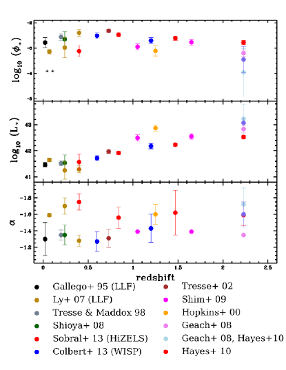
Figure 23: H$\alpha$ LF as estimated in various surveys. The uncertainties on the different parameters defining the LF are considerable. The aim of this project is to measure the most precise H$\alpha$ and [OIII] luminosity functions to-date, in the redshift range 0.7-1.6 and 2-2.2 respectively.

Above z=1.6, the H$\alpha$ line is redshifted outside the detectable wavelength range and since single line emitters are considered H$\alpha$ by default, the ability to confirm the identification of [OIII] lines is limited to bright lines with clear shapes. Greatly extending the small dataset used in Colbert et al. (2013), the newly released WISP data will allow us to better constrain the contamination of the H$\alpha$ selected sample, and the loss of completeness of the [OIII] sample. We will use the multi-wavelength dataset on 3D-HST + AGHAST to identify a combination of colors that could possibly mitigate this problem.

The identification of the spectral lines and the measure of their fluxes is fundamental for all the successive part of the LF project here described, but it can not be completely performed by an automatic algorithm. Thanks to the same collaboration involving both the SIT and WISP team members, automatic softwares have already been optimized to i) remove low S/N detections and some of the contaminating false detections and ii) measure the total line fluxes after their identification. However, the human interaction is required to visually identify each detected line (mostly H$\alpha$ and [OIII], but also OII, H$\beta$ and SII), to perform high quality continuum and line fits, and to remove not automatically identified contaminants. In the past weeks, the work has been focused on these tasks. As a result, a large dataset of thousands of objects with measured line fluxes and corresponding redshift is now available.

At the end of the work described in this section, for which more than a semester is still reasonably required, the results will lead to a publication in one of the major journals, with the co-authorship of Teplitz, Baronchelli and Wang.

5.4 Cosmological Forecasting and Data Analysis Algorithms (D4)

We have developed software package to make quick forecasts on basic dark energy parameters from higher order statistics, incluging power spectrum and bispectrum multipoles. This light and agile software package will be the backbone of our GRS proto-pipeline effort.

The key dark energy constraints from the WFIRST GRS will result from the BAO and RSD measurements from the two-point statistics of the observed galaxy field. Similar measurements from the higher order statistics are weaker and currently are considered less robust. Cosmological constraints from higher order statistics scale very steeply with the number density and since WFIRST GRS will provide very dense galaxy samples they may significantly enhance the yield from the standard two-point BAO/RSD analysis. We also expect the methods of analyzing higher order statistics to become more robust and standardized by the time of WFIRST launch. Because of these considerations it would be helpful to have a higher order statistics forecasting tool. We have developed software package to make forecasts on basic dark energy parameters from higher order statistics. The main assumptions are similar to the ones made in the standard power-spectrum forecasting tool used for baseline WFIRST predictions. We will work on integrating this software with the standard forecasting tool developed by our SIT. While the key design decisions will still be based on the two-point statistics forecasts, knowing how different choices will effect higher order analysis will be very informative.

The KSU group has assembled a fast and lightweight set of tools for analyzing the WFIRST GRS data. Currently this toolset starts from the redshift catalogue and the visibility cube and produces the measurements of power spectrum multipoles. The multipoles are then analyzed to extract the BAO and RSD signal from them. The BAO extraction algorithms replicate the analysis of the final BOSS DR12 sample. The RSD analysis is currently simplistic and uses the linear model. We will update this toolset by implementing more realistic RSD models. The toolset will eventually be linked to the redshift catalogue and visibility cube producing software. This software will provide the backbone of our BAO/RSD proto-pipeline and will be validated with high fidelity WFIRST simulations.

[]

1. We will keep refining and solidifying the scientific requirements;

2. We will pursue our light-cone simulations and release mock catalogs to the community when publishing our results;

3. We will pursue our effort with image simulation, relying on the light-cone simulation to incorporate realistic galaxy distributions and properties;

4. We will continue our pseudo-pipeline effort;

6 Cosmological Forecasts (D2, D6, D7)

We developed a unique and coherent cosmological forecast software package, CosmoLike . Using this single unified framework, we revised the HLSS and HLIS cosmological forecasts, including systematics effects. We also pioneered a joint HLSS-HLIS analysis. This led us to emphasize the importance and the power of a multi-probe cosmological approach. We also performed several trade studies to support Project Office activities, in conjunction with the SNe SITs.

In this section we will describe the results a simulated likelihood analysis that forecasts science return and quantified systematics for different choices in the WFIRST HLS survey. We first introduce the CosmoLike software framework that was used to generate our forecasts. We then present forecasts for HLSS and HLIS specific observables. We conclude with a summary of ongoing research to explore WFIRST multi-probe analysis strategies, i.e., to combine all WFIRST observables and their correlated systematics consistently in simulated likelihood analyses. We also present ongoing work that will assess synergies between WFIRST and other contemporary surveys, e.g., the ground-based, optical Large Synoptic Survey Telescope (LSST) and future missions studying the Cosmic Microwave Background, e.g. CMB-Stage4 (CMB-S4) experiments.

6.1 CosmoLike Introduction

CosmoLike is unique in its approach that jointly models LSS probes as well as their correlated systematics. It is the only code that computes multi-probe covariances, including the (dominant) higher-order terms of the matter density field.

CosmoLike has been used in several science efforts, e.g. the combined probes forecasts presented in (Eifler et al., 2014), an analysis of SDSS shear data (Huff et al., 2014), and efforts to develop new mitigation strategies for baryonic physics (Eifler et al., 2015) and galaxy intrinsic alignment (Krause et al., 2016). It is one of two cosmology analysis pipelines used by the ongoing Dark Energy Survey’s Year 1 analysis and it has previously been used in the DES science verification data analysis (The Dark Energy Survey Collaboration et al., 2015). Beyond DES,

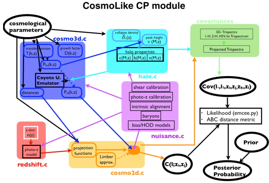
Figure 24: Illustration of a subset of CosmoLike’s code structure. Starting from cosmological parameters we show how different parts of the code interface and how projected summary statistics for various observables are obtained. This particular workflow corresponds to the multi-probe analysis as described in Sect. 6.4. For the HLSS survey a subset of these routines are being used.

the code has been used to simulate a realistic multi-probe likelihood analyses for LSST (Krause and Eifler, 2017) that include cosmic shear, galaxy clustering, galaxy-galaxy lensing, cluster number counts and cluster weak lensing. The software relies on a massively parallelized computation of fine-tuned look-up tables with a targeted sub-second run-time per point in parameter space. Given the large number of parameters describing systematic effects in future LSS analyses, this efficient computation ensures an acceptable turnaround time for analyses. In particular, it allows one to generate a large number of simulated likelihood analyses which is necessary to optimize future surveys. Figure 24 illustrates the CosmoLike combined probes module we plan to use for the proposed analysis. Starting from a cosmological model, this schematic illustrates how projected power spectra for various LSS probes are computed:

1. In the first step CosmoLike computes the 3D-density power spectrum using one of 3 different methods. The density power spectrum can be modeled using the latest suites of numerical simulations, i.e. the Coyote Universe emulator (Heitmann et al., 2014), or the latest implementation of Halofit (Takahashi et al., 2012), or using a state-of-the-art analytic halo model (Krause et al., 2013).

2. Given a survey specific redshift distribution CosmoLike computes projected (tomographic) 2D power spectra for WL, galaxy-galaxy lensing, and galaxy clustering.

3. For galaxy-galaxy lensing and galaxy clustering, the connection between dark and luminous matter is modeled using either a linear bias model or a sophisticated (but computationally slower) HOD model (Krause et al., 2013).

4. The covariance is computed analytically using perturbation theory to include the higher-order moments of the density field, including the Halo Sample Variance contribution that dominates the statistical error budget. This covariance takes all cross-correlations between the different probes into account.

5. CosmoLike has various systematics modeling capabilities, in particular it can account for baryonic effects, intrinsic alignment, shear calibration and photo-z uncertainties (Eifler et al., 2015; Krause et al., 2016; Krause and Eifler, 2017).

6. If one chooses to use two-point correlation functions instead of power spectra CosmoLike offers an extremely fast Fourier transformation using a Hankel transform. The code employs a parallel MCMC sampling technique (Goodman and Weare, 2010), implemented using the emcee python package (Foreman-Mackey et al., 2013).

6.2 HLS Spectroscopic Survey Forecasts and Trade Studies

We implemented in the CosmoLike package a state of the art spectroscopic survey forecasting formalism. We used this tool to update the HLSS forecast and to conduct two trade studies. We validated and explored the validity of science requirements HLSS1 and HLSS3. (§ 5.1.1).

1. We carried out a trade study of area versus depth for the HLSS only, starting from a baseline survey of 2,227 sq. deg. and a wavelength range of 1.05-1.85 microns. We considered two alternative scenarios, i.e., a survey twice as wide and a survey half as wide but correspondingly deeper.

2. We examined the impact of an extended wavelength range on the cosmological constraining power.

6.2.1 Varying the HLSS Area

The galaxy redshift distributions were computed using the WFIRST Exposure Time Calculator ETC v14. The H$\alpha$ forecasts are based on the average of the 3 models in Pozzetti et al. (2016), and the [O III] forecasts are based on the Mehta et al. (2015) luminosity function. The resulting redshift distributions are displayed in Figure 25 (left panel). We extended the CosmoLike framework (Eifler et al., 2014; Krause and Eifler, 2017) to compute the constraining power of all cosmic acceleration scenarios, closely following Wang et al. (2013). We ran a 500,000 step MCMC simulated likelihood analysis in a 23 dimensional parameter space. We simultaneously varied 7 cosmological parameters and 16 nuisance parameters describing uncertainties due to the linear galaxy bias model, the non-linear smearing of the BAO feature, peculiar velocity dispersion, power spectrum shot noise, and redshift errors. We assumed priors on cosmological parameters from the current state of the art experiments, i.e. the Planck mission, the Baryon Oscillation Spectroscopic Survey, the Joint Lightcurve Analysis, as described in Aubourg et al. (2015).

The information gain is quantified using the standard Dark Energy Task Force FOM and an extended cosmology FOM, which measures the enclosed volume in the full 7-dimensional cosmological parameter space, not just in the 2 dark energy parameters. We will refer to these FOMs as DE-FOM and Cosmo-FOM. Compared to our baseline scenario we find a decreased DE-FOM of 32% and a decreased Cosmo-FOM of 45% for the shallow/large area survey. For the deep/small area survey we find an increased DE-FOM of 5% and an increased Cosmo-FOM of 2%. We note that these findings are model and prior dependent and recommend further studies to confirm these forecasts. We also note that the [O III] numbers are pending a future update in part due to the reduction in the baseline telescope temperature to 260 K.

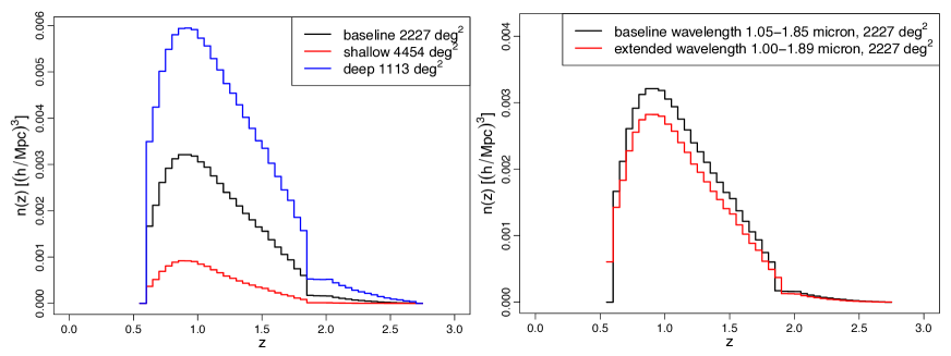
Figure 25: Left:Redshift distribution of galaxies in the baseline, the shallow/large area, and the deep/small area survey. Right: Redshift distribution of galaxies in the baseline and extended wavelength survey.

6.2.2 Varying the HLSS Redshift Coverage

In addition to the trade studies in HLSS 1 we examined the impact of an extended wavelength range on the DE-FOM and the Cosmo-FOM. We follow the same procedure as detailed in the HLSS 1 paragraph extending the wavelength range from 1.05-1.85 microns for the baseline model to 1.00-1.89 for the extended model. The corresponding redshift distributions of the galaxy samples computed from the ETC v1.14 are depicted in Figure 25 (right panel). We find a decreased DE-FOM of 2% and a decreased Cosmo-FOM of 11% for the extended wavelength survey with respect to our baseline scenario. We iterate that these findings are model and prior dependent and recommend further studies varying the input parameters.

6.3 HLS Imaging Survey Forecasts

We extended the CosmoLike package to accurately forecast the HLIS weak gravitational lensing signal, including multiple additional systematics. This extension was then used to study multiple modifications to the survey and its requirements with a focus on the effect of systematics. In particular, we studied

1. The science gain when extending the survey to 10,000 deg², instead if 2,200 deg²;

2. The combined impact of uncertainties in shape and photo-$z$ measurements;

3. The impact of uncertainties in shape measurements only;

4. The impact of uncertainties in photo-$z$ estimation only;

5. The impact of uncertainties in baryonic physics modeling;

6. The impact of uncertainties in intrinsic alignment modeling.

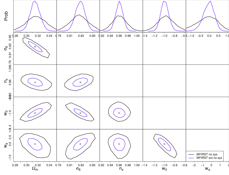
Figure 26: Top: WFIRST forecasts: statistical errors. Extended 10,000 $\mathrm{deg^{2}}$ mission in blue, regular 2,200 $\mathrm{deg^{2}}$ mission in black. Bottom: Broadening of WFIRST error bars accounting for shear calibration and photo-z errors.

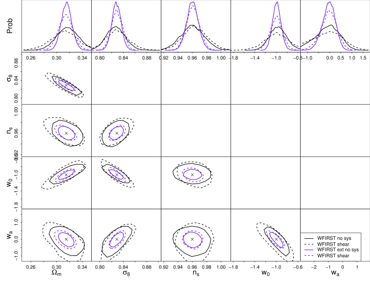
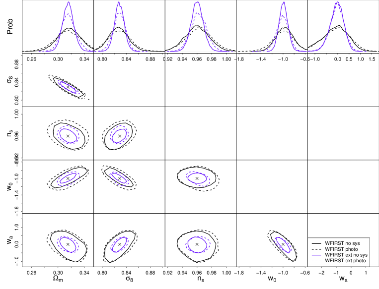
Figure 27: Top: WFIRST statistical errors (solid) compared to errors when including uncertainties from multiplicative shear calibration errors (dashed). Extended 10,000 $\mathrm{deg^{2}}$ mission in blue, regular 2,200 $\mathrm{deg^{2}}$ mission in black Bottom: WFIRST contours when accounting for photo-$z$ uncertainties; see text for details.

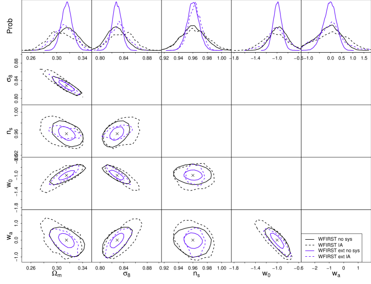
Figure 28: Increase of WFIRST (nominal and extended mission) error bars when marginalizing over intrinsic alignment nuisance parameters (see Krause et al., 2016, for comparison).

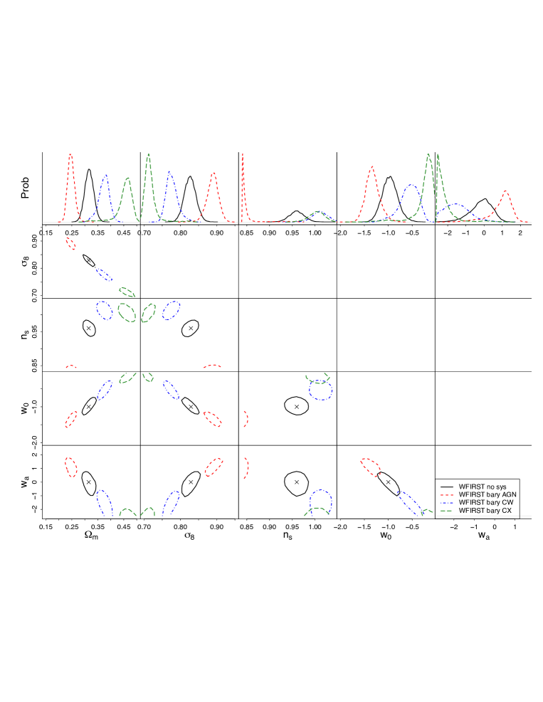
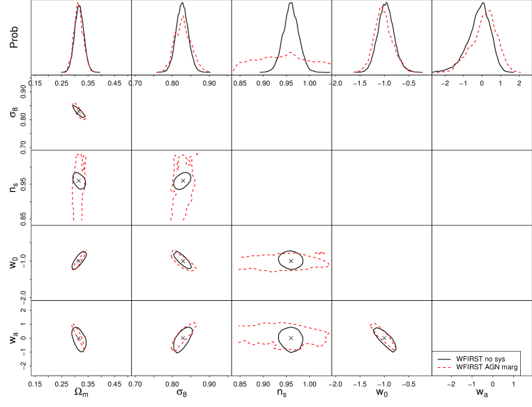
Figure 29: Increase of WFIRST (nominal and extended mission) error bars when marginalizing over nuisance parameters modeling baryonic physics (see Eifler et al., 2015, for details of the method).

6.3.1 Modeling Weak lensing observables and covariances

We begin this WFIRST HLIS section by forecasting the weak lensing science component only. We closely follow the weak lensing part of the forecasting machinery described in Krause and Eifler (2017).

6.3.1.1 Shear Tomography Power Spectra

CosmoLike obtains matter power spectra through calls to the Boltzmann CLASS code and it uses the Takahashi et al. (2012) calibration of the halofit fitting function for the non-linear matter power spectrum (Smith et al., 2003). Time-dependent dark energy models ($w=w_{0}+(1-a)\,w_{a}$) are incorporated following the recipe of icosmo (Refregier et al., 2011), which in the non-linear regime interpolates Halofit between flat and open cosmological models (also see Schrabback et al., 2010, for more details).

Having obtained the density power spectra we calculate the shear power spectra as

$$C^{ij}(l)=\frac{9H_{0}^{4}\Omega_{\mathrm{m}}^{2}}{4c^{4}}\int_{0}^{\chi_{\mathrm{h}}}\mathrm{d}\chi\,\frac{g^{i}(\chi)g^{j}(\chi)}{a^{2}(\chi)}P_{\delta}\left(\frac{l}{f_{K}(\chi)},\chi\right)\,,$$ (16)

with $l$ being the 2D wave vector perpendicular to the line of sight, $\chi$ is the comoving coordinate, $\chi_{\mathrm{h}}$ is the comoving coordinate of the horizon, $a(\chi)$ is the scale factor, and $f_{K}(\chi)$ the comoving angular diameter distance (throughout set to $\chi$ since we assume a flat Universe). The lens efficiency $g^{i}$ is defined as an integral over the redshift distribution of source galaxies $n(\chi(z))$ in the $i^{\mathrm{th}}$ tomographic interval

$$g^{i}(\chi)=\int_{\chi}^{\chi_{\mathrm{h}}}\mathrm{d}\chi^{\prime}n^{i}(\chi^{\prime})\frac{f_{K}(\chi^{\prime}-\chi)}{f_{K}(\chi^{\prime})}\,.$$ (17)

Since we chose five tomographic bins, the resulting data vector which enters the likelihood analysis consists of 15 tomographic shear power spectra, each with 12 logarithmically spaced bins ($l\in[100;5000]$), hence 180 data points overall. The limits of the tomographic $z$-bins are chosen such that each bin contains a similar number of galaxies.

6.3.1.2 Shear Covariances

Under the assumption that the 4pt-function of the shear field can be expressed in terms of 2pt-functions (so-called Gaussian shear field) the covariance of projected shear power spectra can be calculated as in (Hu and Jain, 2004)

$$\mathrm{Cov_{G}}\left(C^{ij}(l_{1})C^{kl}(l_{2})\right)=\langle\Delta C^{ij}(l_{1})\,\Delta C^{kl}(l_{2})\rangle=\frac{\delta_{l_{1}l_{2}}}{2f_{\mathrm{sky}}l_{1}\Delta l_{1}}\left[\bar{C}^{ik}(l_{1})\bar{C}^{jl}(l_{1})+\bar{C}^{il}(l_{1})\bar{C}^{jk}(l_{1})\right]\,,$$ (18)

with

$$\bar{C}^{ij}(l_{1})=C^{ij}(l_{1})+\delta_{ij}\frac{\sigma_{\epsilon}^{2}}{n^{i}}\,,$$ (19)

where the superscripts indicate the redshift bin; $n^{i}$ is the density of source galaxies in the $i$-th redshift bin; and $\sigma_{\epsilon}$ is the RMS of the shape noise.

Since non-linear structure growth at late time induces significant non-Gaussianities in the shear field, using the covariance of Eq. (18) in a likelihood analysis results in an underestimate of the errors on cosmological parameters. Therefore, the covariance must be amended by an additional term, i.e. $\mathrm{Cov}=\mathrm{Cov_{G}}+\mathrm{Cov_{NG}}$. The non-Gaussian covariance is calculated from the convergence trispectrum $T_{\kappa}$ (Cooray and Hu, 2001; Takada and Jain, 2009), and we include a sample variance term $T_{\kappa,\rm{HSV}}$ that describes scatter in power spectrum measurements due to large scale density modes (Takada and Bridle, 2007; Sato et al., 2009),

$$\mathrm{Cov_{NG}}(C^{ij}(l_{1}),C^{kl}(l_{2}))=\int_{|\mathbf{l}|\in l_{1}}\frac{d^{2}\mathbf{l}}{A(l_{1})}\int_{|\mathbf{l}^{\prime}|\in l_{2}}\frac{d^{2}\mathbf{l}^{\prime}}{A(l_{2})}\left[\frac{1}{\Omega_{\mathrm{s}}}T_{\kappa,0}^{ijkl}(\mathbf{l},-\mathbf{l},\mathbf{l}^{\prime},-\mathbf{l}^{\prime})+T_{\kappa,\rm{HSV}}^{ijkl}(\mathbf{l},-\mathbf{l},\mathbf{l}^{\prime},-\mathbf{l}^{\prime})\right]\,,$$ (20)

with $A(l_{i})=\int_{|\mathbf{l}|\in l_{i}}d^{2}\mathbf{l}\approx 2\pi l_{i}\Delta l_{i}$ the integration area associated with a power spectrum bin centered at $l_{i}$ and width $\Delta l_{i}$.

The convergence trispectrum $T_{\kappa,0}^{ijkl}$ (in the absence of finite volume effects) is defined as

$$T_{\kappa,0}^{ijkl}(\mathbf{l}_{1},\mathbf{l}_{2},\mathbf{l}_{3},\mathbf{l}_{4})=\left(\frac{3}{2}\frac{H_{0}^{2}}{c^{2}}\Omega_{\mathrm{m}}\right)^{4}\int_{0}^{\chi_{h}}{\rm d}\chi\,\left(\frac{\chi}{a(\chi)}\right)^{4}g^{i}g^{j}g^{k}g^{l}\times\chi^{-6}\,T_{\delta,0}\left(\frac{\mathbf{l}_{1}}{\chi},\frac{\mathbf{l}_{2}}{\chi},\frac{\mathbf{l}_{3}}{\chi},\frac{\mathbf{l}_{4}}{\chi},z(\chi)\right)\,,$$ (21)

with $T_{\delta,0}$ the matter trispectrum (again, not including finite volume effects), and where we abbreviated $g^{i}=g^{i}(\chi)$.

We model the matter trispectrum using the halo model (Seljak, 2000; Cooray and Sheth, 2002), which assumes that all matter is bound in virialized structures that are modeled as biased tracers of the density field. Within this model the statistics of the density field can be described by the dark matter distribution within halos on small scales, and is dominated by the clustering properties of halos and their abundance on large scales. In this model, the trispectrum splits into five terms describing the 4-point correlation within one halo (the one-halo term $T^{\mathrm{1h}}$), between 2 to 4 halos (two-, three-, four-halo term), and a so-called halo sample variance term $T_{\mathrm{HSV}}$, caused by fluctuations in the number of massive halos within the survey area,

$$T=T_{0}+T_{\mathrm{HSV}}=\left[T_{\mathrm{1h}}+T_{\mathrm{2h}}+T_{\mathrm{3h}}+T_{\mathrm{4h}}\right]+T_{\mathrm{HSV}}\;.$$ (22)

The two-halo term is split into two parts, representing correlations between two or three points in the first halo and two or one point in the second halo. As halos are the building blocks of the density field in the halo model approach, we need to choose models for their internal structure, abundance, and clustering, in order to build a model for the trispectrum.

Our implementation of the one-, two- and four-halo term contributions to the matter trispectrum follows Cooray and Hu (2001), and we neglect the three-halo term as it is subdominant compared to the other terms at the scales of interest for this analysis. Specifically, we assume NFW halo profiles (Navarro et al., 1997) with the Bhattacharya et al. (2011) fitting formula for the halo mass–concentration relation $c(M,z)$, and the Tinker et al. (2008) fitting functions for the halo mass function $\frac{dn}{dM}$ and linear halo bias $b(M)$ (all evaluated at $\Delta=200$), neglecting terms involving higher order halo biasing.

Within the halo model framework, the halo sample variance term is described by the change of the number of massive halos within the survey area due to survey-scale density modes. Following Sato et al. (2009), it is calculated as

$$T_{\kappa,\rm{HSV}}^{ijkl}(\mathbf{l}_{1},-\mathbf{l}_{1},\mathbf{l}_{2},-\mathbf{l}_{2})=\left(\frac{3}{2}\frac{H_{0}^{2}}{c^{2}}\Omega_{\mathrm{m}}\right)^{4} \times \int_{0}^{\chi_{\mathrm{h}}}d\chi\left(\frac{d^{2}V}{d\chi d\Omega}\right)^{2}\left(\frac{\chi}{a(\chi)}\right)^{4}g^{i}g^{j}g^{k}g^{l}$$ (23)

$$\times \int dM\frac{dn}{dM}b(M)\left(\frac{M}{\bar{\rho}}\right)^{2}|\tilde{u}(l_{1}/\chi,c(M,z(\chi))|^{2}$$

$$\times \int dM^{\prime}\frac{dn}{dM^{\prime}}b(M^{\prime})\left(\frac{M^{\prime}}{\bar{\rho}}\right)^{2}|\tilde{u}(l_{2}/\chi,c(M^{\prime},z(\chi))|^{2}$$

$$\times \int_{0}^{\infty}\frac{kdk}{2\pi}P_{\delta}^{\mathrm{lin}}(k,z(\chi))|\tilde{W}(k\chi\Theta_{\mathrm{s}})|^{2}\,.$$

6.3.1.3 Cosmological Parameter Studies

Our ability to model shear power spectra and non-Gaussian covariances means that we can forcast cosmological constraints for different survey scenarios. For all forecasts, we sample the joint parameter space of cosmological $\mathbf{p}_{\mathrm{c}}$ and nuisance parameters $\mathbf{p}_{\mathrm{n}}$ and parameterize the joint likelihood as a multivariate Gaussian

$$L(\mathbf{D}|\mathbf{p}_{\mathrm{c}},\mathbf{p}_{\mathrm{n}})=N\,\times\,\exp\biggl{(}-\frac{1}{2}\underbrace{\left[(\mathbf{D}-\mathbf{M})^{t}\,\mathbf{C}^{-1}\,(\mathbf{D}-\mathbf{M})\right]}_{\chi^{2}(\mathbf{p}_{\mathrm{c}},\mathbf{p}_{\mathrm{n}})}\biggr{)}\,.$$ (24)

The model vector $\mathbf{M}$ is a function of cosmology and nuisance parameters, i.e. $\mathbf{M}=\mathbf{M}(\mathbf{p}_{\mathrm{c}},\mathbf{p}_{\mathrm{n}})$ and the normalization constant $N=(2\pi)^{-\frac{n}{2}}|C|^{-\frac{1}{2}}$ can be ignored under the assumption that the covariance is constant in parameter space. The assumption of a constant, known covariance matrix $\mathbf{C}$ is an approximation to the correct approach of a cosmology dependent or estimated covariance (see Eifler et al., 2009; Sellentin and Heavens, 2016, for further details). Given the likelihood function we can compute the posterior probability in parameter space from Bayes’ theorem

$$P(\mathbf{p}_{\mathrm{c}},\mathbf{p}_{\mathrm{n}}|\mathbf{D})\propto P_{r}(\mathbf{p}_{\mathrm{c}},\mathbf{p}_{\mathrm{n}})\,L(\mathbf{D}|\mathbf{p}_{\mathrm{c}},\mathbf{p}_{\mathrm{n}}),$$ (25)

where $P_{r}(\mathbf{p}_{\mathrm{c}},\mathbf{p}_{\mathrm{n}})$ denotes the prior probability.

Equation 25 allows us to simulate realistic likelihood analyses for various survey scenarios. In particular we consider the following scenarios:

• Science gain when extending the survey to 10,000 deg², instead of 2,200 deg² (see Fig 26 top)

• Impact of combined uncertainties in shape measurements and photo-z measurements (see Fig 26 bottom)

• Impact of uncertainties in shape measurements only (see Fig 27 top)

• Impact of uncertainties in photo-z estimation only (see Fig 27 bottom)

• Impact of uncertainties in baryonic physics modeling (see Fig 29 bottom)

• Impact of uncertainties in intrinsic alignment modeling (see Fig 28 bottom)

Shear calibration uncertainties are modeled as a Gaussian with $\sigma=0.005$ in each of the 10 tomographic bins, which altogether leads to 11 nuisance parameters. Redshift errors are modeled as Gaussian errors with a bias around mean zero and $\sigma=0.05$. In each tomographic bin these parameters (bias and $sigma$) again have Gaussian priors, i.e. $\Delta\mathrm{bias}=0.005$ and $\Delta\sigma=0.006$.

For intrinsic alignment we assume the non-linear alignment model, closely following the parameterization and implementation of Krause et al. (2016), i.e. we marginalize over 11 nuisance parameters for amplitude, redshift dependence, and luminosity function uncertainties.

For the impact of baryonic physics modeling, we follow the work of Eifler et al. (2015), where the authors examined the impact of different baryonic scenarios and quantify the bias in cosmological constraints for LSST and DES when the impact of baryons are neglected. We repeat this analysis for WFIRST (Figure 29, upper) and also account for the uncertainties due to baryonic scenarios in a subsequent analysis (Figure 29, lower). There, we project out modes that are sensitive to baryonic physics in our analysis, which comes at the cost of constraining power, in particular the spectral index $n_{s}$. We note, however, that $n_{s}$ is strongly constrained by CMB measurements and that a corresponding prior will recover the lost information.

6.4 Expanding the Science Case - Multi-Probe Forecasts

Using our updates to the CosmoLike package described in the previous sections, we have now implemented a full multi-probe analysis, an extremely promising area of active research. We are able to combine all cosmological probes enabled by WFIRST HLS. This is one of the major goal of our unified HLS SIT. The likelihood analyses presented here are the start of a demanding study to optimally combine WFIRST internal observables and also to study synergies between WFIRST and other, external data sets, in particular LSST. Our tools will enable us to do so in the coming years. We also study new cosmological signals these multi-probe analysis will allow us to measure, such as the effect of primordial non-Gaussianity on galaxy shapes and synergies with CMB lensing.

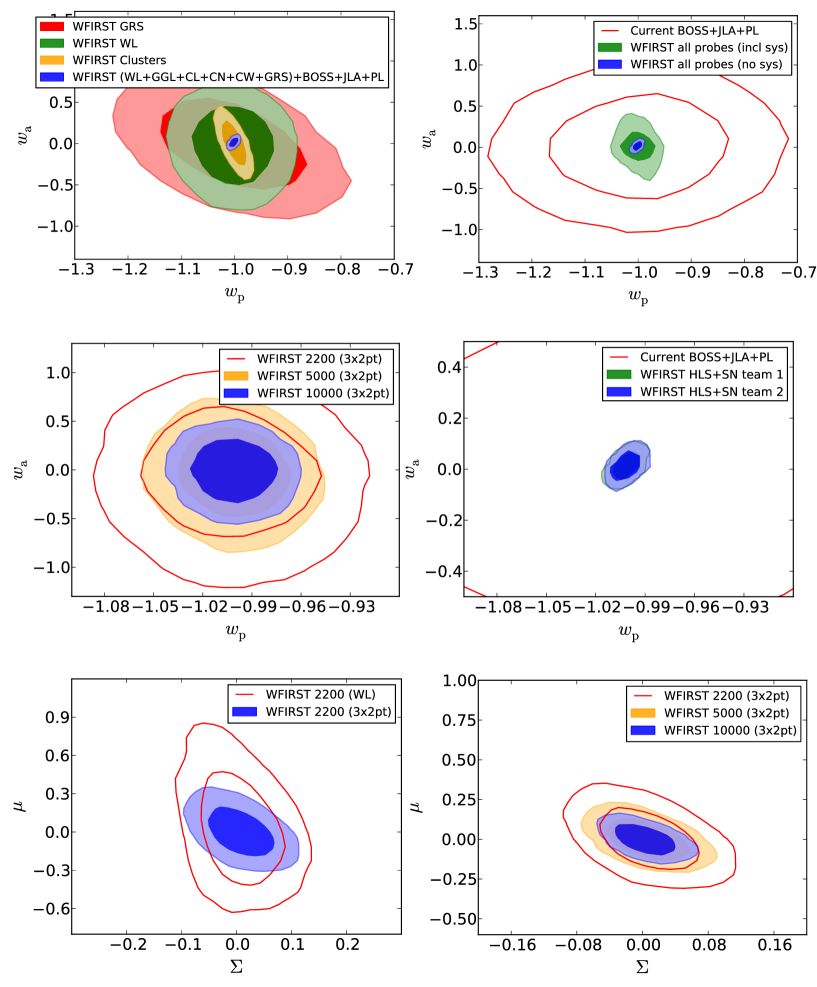
Figure 30: WFIRST multi-probe studies, see text for details.

6.4.1 CosmoLike Multi-probe Analysis

Developing a multi-probe cosmology analysis framework is challenging given that the analysis pipeline for individual probes are each under continuous development in order to meet the requirements of improving data quality. These efforts have historically been largely independent from each other; as a consequence, individual probe analyses utilize information from other probes to offset/calibrate systematics. For example, one of the most important astrophysical uncertainties for galaxy clustering is the relation of dark matter halos and luminous galaxies. The joint analysis of clustering and galaxy-galaxy lensing measurements removes uncertainties in this halo-galaxy connection when constraining cosmology. However, cosmic shear analyses use the same galaxy-galaxy lensing measurements to offset other systematic uncertainties (e.g., intrinsic galaxy alignment). This is only one example of many systematics mitigation conflicts that can occur when considering probes in isolation. A multi-probe analysis framework must account for these correlated systematic effects consistently across all probes; it cannot simply combine the optimal versions of individual analyses and it must include a global, well-designed systematics modeling and mitigation concept.

In this section we present a variety of simulated multi-probe WFIRST analyses. Our results are summarized in Figure 30. The upper left panel shows the constraining power of the individual survey elements (galaxy-redshift survey, weak lensing, galaxy clusters) in comparison to their combined constraining power plus galaxy-galaxy lensing, photometric galaxy clustering, and prior information from Planck, SN1a, BOSS. The likelihood analysis was carried out in a 7-dimensional cosmological parameter space, excluding any systematics. The right panel compares the aforementioned joint analysis (blue) with the current state of the art (red) and we show how the contours increase when including a realistic set of systematics in the analysis. These systematics include uncertainties arising from shear and photo-$z$ calibration, cluster mass-observable relation, galaxy intrinsic alignment, and galaxy bias. Modeling and marginalizing over these systematics requires us to run a likelihood analysis in 54 dimensional parameter space; the details of our analysis are very similar to the LSST forecasts in Krause and Eifler (2017), but for WFIRST survey parameters (survey area, number density, and redshift distribution).

The second row, left panel shows results from a simulated multi-probe analysis that can be extracted from the imaging survey only. The so-called 3$\times$2pt analysis consists of second-order statistics from weak lensing, photometric galaxy clustering, and galaxy-galaxy lensing. We show the scaling of the error bars (statistics only, no systematics) when going from the nominal survey area to a 5,000 and 10,000 deg² survey.

The second row, right panel shows again our full multi-probe analysis including galaxy clusters and the spectroscopic survey component, i.e., BAO and RSD measurements, and we also include information from the 2 WFIRST supernovae teams. These team independently forecasted the WFIRST SN1a constraining power and are in excellent agreement.

The lower row, left panel shows the constraining power of WFIRST weak lensing and 3$\times$2pt for the nominal survey area on modified gravity parameters $\mu$ and $\Sigma$ (see e.g., Joyce et al., 2015; Bull et al., 2015, for details). The right panel shows the constraining power when increasing the survey area again to 5,000 and 10,000 deg². The work on modified gravity extensions of CosmoLike is led by JPL Postdocs Hironao Miyatake and Phil Bull in close collaboration with Tim Eifler and Elisabeth Krause and we plan to extend the results shown in Figure 30 to include further, recent developments in the field of modified gravity parameterization and classification. In particular, we plan to implement the ability to model modified gravity scenarios that belong to the class of Horndeski actions, which is the most general action for a single classical scalar field in the presence of gravity which does not result in any derivatives higher than second order in the equations of motion.

We emphasize that multi-probe studies are an area of active research and that the likelihood analyses presented here represents a first step towards our goal of optimally combining WFIRST internal observables and to study synergies between WFIRST and other, external data sets, in particular LSST.

6.4.2 Other Signals in Multi-Probe Analysis

Spergel and his group have been exploring the use of galaxy shapes to constrain primordial non-Gaussianity (Chisari et al., 2016). Working with former Princeton student, Elisa Chisari, and former Princeton postdocs Cora Dvorkin and Fabian Schmidt, they showed that multi-tracer weak lensing observations could create anisotropic non-Gaussianity. WFIRST will be a powerful instrument for this approach. Correlations between intrinsic galaxy shapes on large-scales arise due to the effect of the tidal field of large-scale structure. Anisotropic primordial non-Gaussianity induces a distinct scale-dependent imprint in these tidal alignments on large scales. Motivated by the observational finding that the alignment strength of luminous red galaxies depends on how galaxy shapes are measured, we study the use of two different shape estimators as a multi-tracer probe of intrinsic alignments. We show, by means of a Fisher analysis, that this technique promises a significant improvement on anisotropic non-Gaussianity constraints over a single-tracer method. For future weak lensing surveys, the uncertainty in the anisotropic non-Gaussianity parameter, $A_{2}$, is forecast to be $\sigma(A_{2})\simeq 50$, $\sim$ 40% smaller than currently available constraints from the bispectrum of the Cosmic Microwave Background. This corresponds to an improvement of a factor of 4−5 over the uncertainty from a single-tracer analysis.

Emmanuel Schaan has been working with Spergel and with the JPL group to explore the use of CMB lensing measurements as a tool to calibrate multiplicative bias (Schaan et al., 2016). WFIRST will require exquisite control over systematic effects. In their paper, they address shear calibration and present the most realistic forecast to date for WFIRST and CMB lensing from a stage 4 CMB experiment (CMB S4). We use the CosmoLike code to simulate a joint analysis of all the two-point functions of galaxy density, galaxy shear and CMB lensing convergence. We include the full Gaussian and non-Gaussian covariances and explore the resulting joint likelihood with Monte Carlo Markov Chains. We constrain shear calibration biases while simultaneously varying cosmological parameters, galaxy biases and photometric redshift uncertainties. We find that CMB lensing from CMB S4 enables the calibration of the shear biases down 0.6-3.2% in 10 bins for WFIRST (see Fig. 31). For a given lensing survey, the method works best at high redshift where shear calibration is otherwise most challenging. This self-calibration is robust to Gaussian photometric redshift uncertainties and to a reasonable level of intrinsic alignment. It is also robust to changes in the beam and the effectiveness of the component separation of the CMB experiment, and slowly dependent on its depth, making it possible with third generation CMB experiments such as AdvACT and SPT-3G, as well as the Simons Observatory.

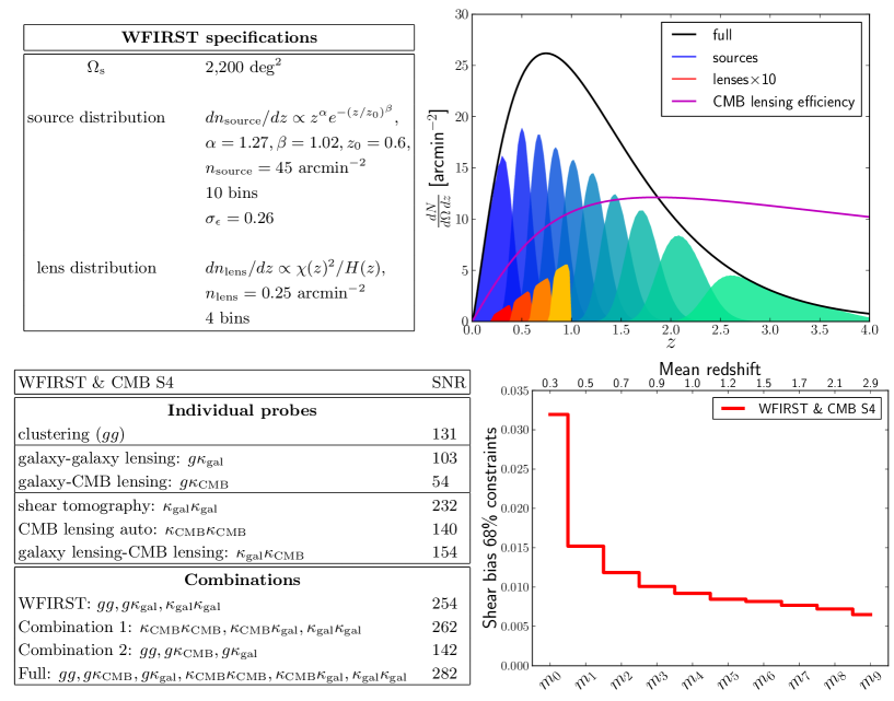
Figure 31: Summary of the forecast for WFIRST and CMB S4 lensing. The top left panel summarizes our assumptions for the WFIRST survey. The top right panel displays the photo-z bins assumed for the lens and source samples. The bottom left panel summarizes the signal to noise ratios for the various probes and combinations. The bottom right panel shows the level of shear calibration in WFIRST’s ten source bins via CMB-S4 lensing. The calibration of the shear biases down 0.6-3.2% in particular at high redshift bins, constitutes a promising alternative and an important cross-check to traditional simulation based approaches.

Relying on our updates to the CosmoLike package, we revised the cosmological forecasts for the HLS spectroscopic and imaging survey. Using the unique CosmoLike capabilities, we conducted for the first time a full HLS multi-probe analysis in which we considered joint constraints between the HLS spectroscopic galaxy sample, the HLS photometric galaxy samples, the HLS weak gravitational shear signal, the HLS galaxy-galaxy lensing, the HLS galaxy clusters samples and the HLS SNe sample. Our approach takes into account correlations between these probes as well as multiple systematic effects associated with each probe. We also combined WFIRST with other external surveys such as Planck and LSST. This is a milestone for our unified HLS SIT and we will investigate further the power and robustness of this multi-probe analysis in the coming years. We used this new capability to conduct trade studies to guide the development of the SRD. We also investigated new cosmological signals enabled by multi-probe studies, such as tests of general relativity.

7 Operations Model for the HLS and Evaluation of Trades (D7, D10, D11)

Co-I Hirata is leading the development of the HLS observing plan, extending his previous tools used for the SDT. These tools incorporate observing constraints in the chosen orbit, an exposure-by-exposure observing sequence optimized with detailed model of overheads, and tiling/coverage maps including field distortions and curved sky effects. These tools treat both imaging and spectroscopy with unified functions and scripts, and are well suited to joint survey optimization when both hardware parameters (e.g., reaction wheel orientations) and the observing program (e.g., depth vs. area) are considered. This effort is coordinated with the scheduling and Design Reference Mission (DRM) Working Groups. We are both providing an example detailed plan for the HLS to the DRM working group, and cross-checking the Project’s spreadsheet-level survey calculators against our simulations. The HLS observing plan is also being transferred to the Calibration Working Group, since the HLS observing strategy feeds directly into the issue of self-calibration.

7.1 Survey Optimization Principles

The key constraint in survey optimization is the limited amount of observational time available, since WFIRST is life-time limited and has multiple science focus areas. For fixed instrumental capabilities and observing time, the primary decisions on survey strategy are the trade between depth and total area, and the balance between imaging and spectroscopy. These decisions are driven by two major considerations:

• Pecision – to maximize the DE science return of WFIRST, taking advantage of synergies with other surveys; and

• Accuracy – tight control of systematic uncertainties, to ensure correct DE measurements.

The combined expertise of our team in WL and GRS enables us to rapidly evaluate these trades.

7.1.0.1 HLIS

The statistical power of a WL survey scales with the total number of galaxy shape measurements, the product of the survey area and the effective surface density. The SDT2015 report adopts an HLS imaging exposure time that yields roughly equal contributions from read noise and sky noise in the most sensitive filters, which approximately maximizes the total number of shape measurements. This is a compromise between minimizing overheads and read noise (which favors a “deep” mode), versus the shallow number counts of resolved WL sources (shallower than $N\propto F^{-2}$, which favors a “wide” mode). We re-examined the depth vs. area trade using higher-fidelity tools (e.g., incorporation of shape measurement noise from realistic simulations, and updated detector properties) and propagating the trades all the way to cosmological parameters (using CosmoLike ).

7.1.0.2 HLSS

The depth vs. area trade for the GRS is driven by two competing factors: for deep surveys, where the number density of galaxies $n$ is large ($nP\gg 1$, where $P$ is the power spectrum at a given scale), the information per unit area saturates; whereas for wide surveys, overheads reduce inefficiency and galaxy shot noise inflates the statistical errors. In the SDT15 survey design, the GRS covers the same area as the HLS imaging survey ($\approx 2,200\,{\rm deg}^{2}$), to a $7\sigma$ limiting line flux of $\sim 10^{-16}\,{\rm erg}\,{\rm cm}^{-2}\,{\rm s}^{-1}$ over most of the grism bandpass. This yields approximately the largest number of galaxy redshifts for a fixed total observing time. SDT15 found that doubling the survey area at fixed observing time (even without additional imaging) reduces the precision of BAO measurements because of the rapid increase in galaxy shot noise with decreasing spectroscopic depth. However, this conclusion is sensitive to the luminosity function of H$\alpha$ emitters at $z=1-2$, which remains uncertain Mehta et al. (2015); Pozzetti et al. (2016); Co-Is Teplitz and Wang lead our efforts to reduce this uncertainty and feed the results into optimization of the GRS (§ 5.3).

7.2 Snapshot of the HLS observing plan

Our team provided a “snapshot” of the HLS observing sequence to the full FSWG on April 19, 2017. This is by no means a final or even optimized version of the HLS, but is a work in progress as a result of trades in Phase A, as well as the recent decision to reduce the primary mission to 5 years.

Major updates relative to the SDT plan have included:

• A Lissajous orbit around L2. This is presently a place-holder, as the exact orbit has not yet been selected (and would depend on the launch date), but it gives a possible sampling of Sun, Earth, and Moon constraints.

• A rotated WFI (by 90^∘ relative to the Cycle 6 design).

• Recommended slew and settle times provided by the Project.

• Faster detector readout (200 kHz instead of 100 kHz).

• Changes to the exposure time and dithering strategy to accommodate a 5-year baseline mission (as is to be presented to the WIETR). Specifically, we reduced exposure time to 140.2 s (imaging) and 297.0 s (spectroscopy); and changed the dither pattern in J band. (We are working on checking this strategy with image simulations, if it causes a problem we may have to revert.)

• Implemented bright star avoidance (observations are skipped if there is an $H_{\rm AB}\leq 3$ star within 6 arcmin of any SCA).

Known current issues with the snapshot plan include:

• The SN and coronagraph programs in the code haven’t been updated since the SDT (except to cut the mission time by a factor of 5/6), even though they will likely change significantly. As in the SDT report, the coronagraph has blocks of time reserved. This will evolve in order to align the HLS plan with the other groups, as well as any changes to the scheduling architecture that we are directed to implement (e.g. block scheduling).

• We have begun putting the deep fields into this document, but right now they are (i) not fully specified, (ii) the tiling is not optimized, and (iii) some roll angles don’t align with WFIRST constraints (hence didn’t schedule). These issues will be solved in the next snapshot.

We note that no policy decisions should be inferred from this sequence, as these will come from a higher level.

The survey bounding box is 2,097 deg². The area covered with $\geq 3$ exposures in every filter and the grism, including edge effects and holes around the bright stars, is 1,947 deg². The time required for this version of the HLS is 394 days (imaging) + 215 days (spectroscopy).

The scheduling tools output a set of charts, included in this package:

• Fig. 32: Graphical display of the 5-year observing sequence.

• Fig. 33: HLS distribution of number of exposures in each filter.

• Fig. 34: HLS distribution of dust column [$E(B-V)$ in magnitudes]. Cosmological forecasts are based on a dust column of $E(B-V)=0.035$ mag.

• Fig. 35: HLS distribution of zodiacal light (normalized to 1 at the ecliptic poles averaged over the year). Cosmological forecasts are based on a zodiacal brightness of 1.60 (except for 1.75 in the F184 filter, which is the least sensitive to zodiacal light and therefore was scheduled at inferior times of year).

• Fig. 36: The footprint of the HLS on the sky. This is an area of ongoing optimization, as we consider the needs of the deep fields, overlap with LSST, and the fraction of the survey footprint accessible from Northern observatories such as Subaru.

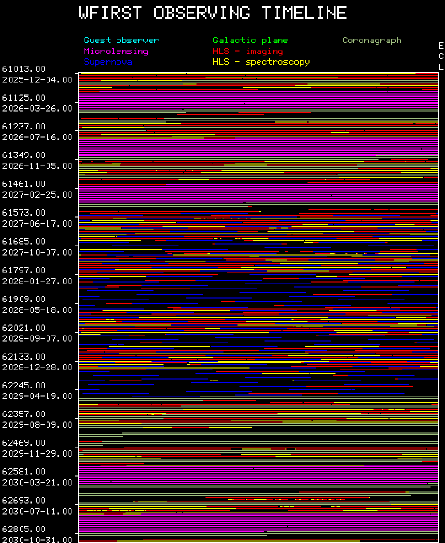
Figure 32: Observing timeline. Each row represents 7 days of observations, and is color-coded according to the observing program. Note the microlensing seasons (magenta), supernova survey (blue: $\sim$5-day cadence), and HLS (red+yellow). Blank areas are not allocated. Labels on the left-hand side are shown every 16 weeks.

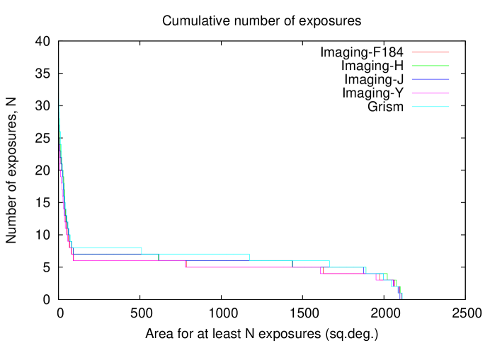
Figure 33: The cumulative distribution of HLS exposure depths above a certain area. The pile-up with many exposures at small area is the result of the deep fields.

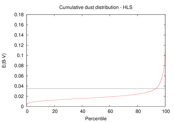
Figure 34: The cumulative distribution of Galactic dust in the HLS.

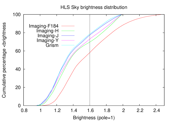
Figure 35: The cumulative distribution of zodiacal light in the HLS.

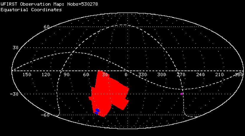
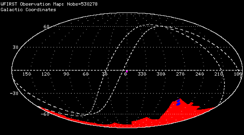
Figure 36: The footprint of the HLS (red) in Equatorial (top) and Galactic (bottom) coordinates.

7.3 Further optimizations

Our team plans to study further optimizations to the HLS – including more drastic changes such as multi-tiered surveys, or a significant re-balancing of area vs. depth – in Phase B. However, in preparation for SRR/MDR, our main focus has been on demonstrating at least one survey configuration that meets requirements, and the construction of tools that link the observing strategy to calibration studies (§4.2) and image simulations (§4.3.4).

The optimization of the WFIRST HLS will be tightly linked to operations simulations, which inform the possible range of footprint area and location, depth in each filter (or grism), redundancy, and temporal distribution of exposures. We propose a highly integrated approach, with the operations simulations at the core, but with links to pixel-level simulations to assess required redundancy, cosmological forecasting tools (CosmoLike ) to assess science reach, and comparison to the observing regions of other surveys and telescopes to maximize synergies and meet requirements for deep fields and photo-$z$ calibration.

8 Community Engagement and External Data-sets (D10, D11, D12)

The coming decade will be an exciting time for cosmology. Before WFIRST launch, major cosmological imaging surveys (KiDS, HSC, DES) and the DESI and PFS spectroscopic surveys will significantly advance our current understanding. WFIRST, Euclid and LSST will then go further and survey the sky at optical and infrared wavelengths, the James Webb Space Telescope (JWST) and the Extremely Large Telescopes (ELTs) will make very deep maps of the sky; eROSITA will survey the X-ray sky; CMB-S4 will make a deep map of the millimeter sky; and the Canadian Hydrogen Intensity Mapping Experiment (CHIME) and other radio surveys will map the large-scale distribution of H i. One goal of our SIT is to determine the analysis infrastructure and observations needed to achieve the full potential of WFIRST in combination with these surveys. This is best done through a broad community effort that brings together scientists from these complementary projects. For this purpose, we organized a first community workshop focused on enabling the cosmological scientific synergies between WFIRST and LSST.

Our SIT naturally brings close connections to most of the major current or planned cosmological experiments that will provide the context for the WFIRST dark energy program. This includes the WMAP and Planck CMB missions, the Sloan Digital Sky Survey (SDSS), the Baryon Oscillation Spectroscopic Survey (BOSS), the Dark Energy Survey (DES), the Subaru Hyper Suprime-Cam (HSC) and Prime Focus Spectrograph (PFS) projects, the Dark Energy Spectroscopic Instrument (DESI), the Euclid mission and the Large Synoptic Survey Telescope (LSST) Dark Energy Science Collaboration (DESC).

We also started to actively engage the community to identify and pursue the key areas where WFIRST and the concurrent projects will provide new opportunities to mitigate systematics and enhance the combined cosmological science return. We started a series of open community workshops to incorporate the interplay between major planned surveys and WFIRST into the WFIRST strategy, to identify: (i) pre-launch observations, (ii) how these external data sets affect the WFIRST observing strategy (e.g., deep fields) and the instrument, and (iii) the software needed (to be built post-CDR) for combining these data sets.

First Community Workshop

The first of this meeting happened in Pasadena in September 2016. It was focused on the synergies between the WFIRST HLS Cosmology SIT and LSST Dark Energy Science Collaboration (DESC), both at the science level but also at the implementation level. The meeting was co-organized by Rachel Bean, Olivier Doré, Steve Kahn and Jason Rhodes and was attended by about 60 scientists from the two collaborations. The slides are available here and pictures can be seen in Figure 37. The conclusion of the lively and productive workshop will be summarized in a white paper to be written shortly.

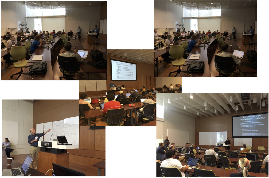
Figure 37: Pictures taken during the Pasadena WFIRST SIT - LSST DESC workshop on September 2016.

Premise

The workshop was built on the premise that when considering joint science return from LSST and WFIRST, the whole is greater than the sum of the parts, as already articulated in Jain et al. (2015). In the conclusion of the Jain et al. community white paper, it was articulated that the scientific opportunity offered by the combination of data from LSST and WFIRST (and Euclid) goes well beyond the science enabled by any one of the data sets alone. The range in wavelength, angular resolution and redshift coverage that these missions jointly span is remarkable. With major investments in LSST and WFIRST (and partnership with ESA in Euclid), the US has an outstanding scientific opportunity to carry out a combined analysis of these data sets. It is imperative for us to seize it and, together with our European colleagues, prepare for the defining cosmological pursuit of the 21st century.

As illustrated already in § 6, the coming decade will be the era of multi-probes/multi-survey science. The richer insights will come from combining multiple probes (WL, GRS, GC) reliably. If done properly, multiple survey joint analysis will enable new calibration schemes (photo-$z$, intrinsic alignment models, etc.) and new control of systematics (PSF effects, contaminant control such as stars or interlopers).

Joint Analysis

The main argument for conducting a single, high-quality reference co-analysis exercise and carefully documenting the results is the complexity and subtlety of systematics that define this co-analysis. Falling back on many small efforts by different teams in selected fields and for narrow goals will be inefficient, leading to significant duplication of effort. For much of the science, we will need to combine the photometry across multiple wavelengths with varying spectral and spatial resolution – a technical challenge. The joint analysis can be carried out in ways that have different computational demands. The most technically demanding joint analysis is to work with pixel level data of the entire area of overlap between the surveys. Many of the goals of a joint analysis require such a pixel-level analysis. If pixel-level joint analysis is not feasible, catalog-level analysis can still be beneficial, say to obtain calibrations of the lensing shear or the redshift distribution of galaxies. Hybrid efforts are also potentially useful, for example using catalog level information from space for deblending LSST galaxies, or using only a mutually agreed subset of the data for calibration purposes. However the full benefits of jointly analyzing any two of the surveys can be reaped only through pixel-level analysis (Jain et al., 2015).

Possible Implementation

In the workshop, possible algorithmic implementation of a joint analysis pipeline were discussed independently by Peter Melchior and Michael Schneider. Melchior and Goulding (2016) motivated the need for complex galaxy morphology models and developed the relevant statistical framework. For them, complex models become the norm. They are more flexible and properly behaved. WFIRST benefits from LSST through color-morphology priors. LSST benefits from sharp likelihood peaks in WFIRST bands. LSST benefits from WFIRST through superior resolution. Schneider et al. (2015) have developed a probabilistic image reduction pipeline (forward modeling) motivated by challenges in multi-epoch/multi-telescope combinations. They demonstrated improved shear measurements for LSST using the HST Frontier field as a proxy for WFIRST.

Enabling Synergies

It was recognized in the context of photo-$z$ for example, that cooperation already exist to maximize utility and minimize duplication in spectroscopic calibration samples. Capak and collaborators are building a public calibration catalog for WFIRST and LSST (Masters et al., 2017). Also, relevant information for deep surveys synchronization, is also discussed in this context and others (SNe, shape calibration, grism calibration, guest observations). The detailed requirements for LSST + WFIRST photo-$z$ performance are however still to be articulated.

Computing Needs

Large computing efforts are under way in LSST (DESC) with multiple planned data challenges. Resources available for the scale of simulations required (with possible exception of hydrodynamical simulations) are secured. However, ressources needed for sharing simulations (e.g. Millennium DB) and mock catalogs are required. They have historically greatly 
expanded the use of simulations in a broad range of applications. A 100 TB to 1 PB scale infrastructure simply does not exist and data transfer will be a challenge (10 days for 100 TB at 1 Gb). There is great opportunity for future collaborations (e.g., joint mock catalogs) and investments. Opportunity for collaborations and investments. As we will discuss in §9.5, members of our team are leading and participating in a Tri-Agency Cosmological Simulations (TACS) dedicated to this issue.

Ressources

As already discussed in Jain et al. (2015), the resources required to achieve this additional science are outside of what is currently budgeted for LSST by NSF and DOE, and for WFIRST (or Euclid) by NASA. Funding for this science would most naturally emerge from coordination among all agencies involved, and would be closely orchestrated scientifically and programmatically to optimize science returns. A possible model would be to identify members of the science teams of each project who would work together on the joint analysis. The analysis team would ideally be coupled with an experienced science center acting as a focal point for the implementation, and simultaneously preparing the public release and documentation for broadest access by the community.

Future Workshop

The second in our series of SIT community workshop will happen in the fall 2017 in Pasadena, synchronized with a FSWG, and will identify (and discuss the enabling of) scientific synergies between the HLS and other major surveys across all wavelengths.

9 Other Science Investigation Team Contributions to WFIRST Mission (D11)

Our SIT engaged in multiple activities supporting the WFIRST mission and the Project Office not discussed above. We summarize them here:

1. Our SIT actively participated to two workshops dedicated to the WFI;

2. Our SIT contributed to evaluate the WFIRST Supernova Program;

3. Our SIT partially supported 15 post-doctoral researchers and one graduate student;

4. Our SIT published 13 scientific papers supporting our studies or extending the scientific case of WFIRST;

5. SIT team members are co-leading and participating in the Tri-agency Cosmological Simulation Task Force (TACS);

6. SIT team members are co-leading large observational efforts supporting WFIRST science goals;

7. Our team delivered to the community multiple high-value products and softwares.

9.1 Princeton Meetings Participation

In addition to the active participation by the SIT leads in the 4 FSWG meetings that happened this year, team members participated in two focused so-called Princeton Meetings organized by Prof. Spergel at Princeton University and the newly established Center for Computing Astrophysics (CCA) at the Flatiron Institute in New York, NY. These two meetings were focused respectively on planning the data processing need of the WFI given our collective experience with large astronomical dataset data processing, and ancillary science enabled by the HLS. Team members Lupton, Mandelbaum, Samushia, and von der Linden represented our SIT at these meetings and presented their thoughts on these topics.

9.2 Contributions to Evaluation of the WFIRST Supernova Program

In addition to our work on the HLS cosmology surveys, team members Olivier Doré, Chris Hirata, David Spergel, and David Weinberg all contributed to evaluating strategies and requirements for the WFIRST supernova program, providing a sounding board for the two supernova SITs and synthesizing information for project management. Some of these contributions took place in sessions of the WFIRST FSWG meetings and some in telecons and email exchanges with members of the supernova teams. Weinberg wrote an extensive referee report for the Hounsell et al. paper (from the supernova SIT led by Ryan Foley) on WFIRST supernova strategies. Most importantly, all four investigators participated in the “supernova summit” held at KIPAC in March 2017, reading background material from the teams, participating in a day of presentations and discussions, and writing a report for project management and the supernova SITs.

9.3 Support of Postdoctoral Researchers and Graduate Students

Our team has been very proactive at leveraging our collective involvement in other on-going large scale observational efforts such as the Dark Energy Survey (DES), and the SUBARU Hyper-Suprime Cam (HSC) survey, in addition to the upcoming ESA/NASA Euclid mission and the Large Synoptic Survey Telescope Dark Energy Science Collaboration (LSST DESC) where we have been able to create joint appointments with our WFIRST SIT and have assembled a team of very strong postdoctoral researchers. In particular, the following researchers joined our team and are partially supported by out SIT:

• Ivano Baronchelli (Caltech/IPAC), working with Harry Teplitz on updating measurements of the H$\alpha$ luminosity function using HST data;

• Ami Choi (OSU), working with Chris Hirata and David Weinberg on image simulations for the WL analysis;

• Shoubaneh Hemmati (IPAC/Caltech), working with Peter Capak on defining the photometric redshift requirements of the WFIRST WL investigation;

• Albert Izard (JPL), working with Alina Kiessling on cosmological simulations and the requirements driven by the need to accurately compute covariance matrices;

• Niall MacCrann (OSU), working with Chris Hirata and David Weinberg on image simulations for the WL analysis;

• Elena Massara (LBL), working with Shirley Ho on generating light cone simulations for the GRS survey;

• Alex Merson (Caltech/IPAC), working with Yun Wang and Andrew Benson on generating light cone simulations for the GRS survey;

• Hironao Miyatake (JPL/Caltech), working with Jason Rhodes and Tim Eifler on including modified gravity and observational systematic effects in the cosmological parameter likelihood;

• Andres Plazas Malagon (JPL/Caltech), working with Jason Rhodes and Charles Shapiro on computing requirements on detector imperfections driven by the WL survey;

• Melanie Simet (UCR/JPL), working with Alina Kiessling and Jason Rhodes on the WL analysis;

• Michael Troxel (OSU), working with Chris Hirata and David Weinberg on image simulations for the WL analysis;

• Ying Zu (OSU), working with Chris Hirata and David Weinberg on simulations for the galaxy cluster investigation;

• Chen He Heinrich (JPL), working with Olivier Doré and Tim Eifler (starting in fall 2017);

• Alice Pisani (Princeton), working with David Spergel on void statistics for the GRS survey (starting in fall 2017);

• Hao-Yi ”Heidi” Wu (OSU), working with Chris Hirata and David Weinberg on simulations for the galaxy cluster investigation (starting in fall 2017).

In addition, Arun Kannawadi, a graduate student at CMU supervised by Rachel Mandelbaum has been working on image simulation and shape measurement analysis. He is partially supported by our SIT.

9.4 Relevant Scientific Publications by Team Members

In addition to our work supporting the Project Office, we published our results in scientific journals and made them available on the arXiv. The following 13 scientific papers were published by our team members and were motivated by our studies:

1. Gagrani and Samushia (2017), “Information Content of the Angular Multipoles of Redshift-Space Galaxy Bispectrum”;

2. Pearson et al. (2016), “Optimal weights for measuring redshift space distortions in multitracer galaxy catalogues”;

3. Kalus et al. (2016), “Unbiased contaminant removal for 3D galaxy power spectrum measurements”;

4. Pearson and Samushia (2016), “Estimating the power spectrum covariance matrix with fewer mock samples”;

5. Plazas et al. (2016), “The Effect of Detector Nonlinearity on WFIRST PSF Profiles for Weak Gravitational Lensing Measurements”;

6. Plazas et al. (2017a), ”Nonlinearity and pixel shifting effects in HXRG infrared detectors”;

7. Kobayashi et al. (2015), “Can we use weak lensing to measure total mass profiles of galaxies on 20 kpc scales?”;

8. Masters et al. (2017), “The Complete Calibration of the Color-Redshift Relation (C3R2) Survey: Survey Overview and Data Release 1”;

9. Schaan et al. (2016), “Looking through the same lens: shear calibration for LSST, Euclid & WFIRST with stage 4 CMB lensing”;

10. Chisari et al. (2016), “Multitracing Anisotropic Non-Gaussianity with Galaxy Shapes”;

11. Merson et al. (2018), “Predicting H$\alpha$ emission line galaxy counts for future galaxy redshift surveys”, currently under review by MNRAS.

12. Plazas et al. (2017a), “Nonlinearity and pixel shifting effects in HXRG infrared detectors”, Journal of Instrumentation;

13. Plazas et al. (2017b), “Laboratory measurement of the brighter-fatter effect in an H2RG infrared detector”, Accepted for publication in Publications of the Astronomical Society of the Pacific.

9.5 Participation to the Tri-agency Cosmological Simulation Task Force (TACS)

The computational resources required to produce all of the cosmological simulations required for WFIRST are not yet well defined but they are known to be significant. WFIRST shares common goals with other upcoming cosmological surveys including LSST, Euclid, and DESI, so it makes sense to try to coordinate efforts between these projects. Team members have taken leadership positions in articulating and leading this effort.

Team members Kiessling and Heitmann have been asked to co-chair a Tri-Agency Cosmological Simulations (TACS) task force at the request of the Project leads from WFIRST, LSST, and Euclid. The co-chairs have formulated a charge for TACS that has been approved by the Tri-Agency (NASA, DOE, NSF), Tri-Project (WFIRST, LSST, Euclid) group (TAG). TAG has representation from each of the Agencies and Projects and is responsible for the coordination of joint data processing and cosmological simulations for the three Projects. JPL WFIRST Project Scientist Rhodes represents the WFIRST and Euclid Projects on the TAG, Program Scientist Benford represents NASA for WFIRST and WFI Adjutant (and SIT team member) Spergel represents the WFIRST FSWG. TACS consists of the two chairs, 9 task force members, and an advisory board of 7 people, with representation from WFIRST on the task force, advisory board, and from both of the co-chairs. Team member Mandelbaum is a member of the advisory board and team members Benson, Eifler, and Ho are task force members. EXPO SIT lead Robertson is also a member of the Advisory Board.

The primary goal of TACS is to investigate areas for coordination between WFIRST, LSST, Euclid, and DESI of supercomputing resources, supercomputing infrastructure, cosmological simulations, synthetic sky generation, systematics investigation, and workforce personnel. TACS will report their recommendations directly to TAG and the reports will be made public for transparency. The responsibility for implementing any recommendations or negotiating MOUs lies with the TAG. Work is currently underway in TACS and is anticipated to extend into FY18.

9.6 Participation and Leadership Large Observational Program Supporting WFIRST Science Goals

The WFIRST mission will provide an unprecedented survey (in depth and area) of the extragalactic sky at optical and near infrared wavelengths (0.5-2 $\mu$m). However, data in the 3-5 $\mu$m wavelength range is an essential complement to measure stellar masses at $z>$3, probe the earliest sites of reionization, find the earliest quasars and structures, and see heavily obscured regions of galaxies and AGN. Yet, besides Spitzer, no current or planned future mission is able to conduct deep yet wide area surveys at these wavelengths since JWST will be limited to a few square degrees of imaging over its lifetime. Co-I Capak is leading the Spitzer Legacy Survey (SLS) that will provide 20 square degrees of deep imaging. The Spitzer Legacy Survey enables new science and will improve the cosmological constraints provided by WFIRST mission. The fields were chosen to be some of the most observable for missions at L2 (WFIRST, JWST, and Euclid), the North Ecliptic Pole (NEP) and the Chandra Deep Field South (CDFS). The CDFS in particular is also the target of deep LSST data which will complement WFIRST for photometric redshifts.

Co-I Capak is also co-leading the Complete Calibration of the Color-Redshift Relation (C3R2) survey. As discussed in §4.4, a key goal of WFIRST is to measure the growth of structure with cosmic time from weak lensing analysis over large regions of the sky. Weak lensing cosmology will be challenging: in addition to highly accurate galaxy shape measurements, statistically robust and accurate photometric redshift (photo-$z$) estimates for billions of faint galaxies will be needed in order to reconstruct the three-dimensional matter distribution. The C3R2 survey is designed specifically to calibrate the empirical galaxy color-redshift relation to the Euclid, LSST and WFIRST. The C3R2 survey is obtaining multiplexed observations with Keck (DEIMOS, LRIS, and MOSFIRE), the Gran Telescopio Canarias (GTC; OSIRIS), and the Very Large Telescope (VLT; FORS2 and KMOS) of a targeted sample of galaxies most important for the redshift calibration. C3R2 focuses spectroscopic efforts on under-sampled regions of galaxy color space identified in previous work in order to minimize the number of spectroscopic redshifts needed to map the color-redshift relation to the required accuracy. Initial results include the 1283 high confidence redshifts obtained in the 2016A semester and released as Data Release 1 (Masters et al., 2017).

9.7 Community Deliverables

Throughout our studies, our SIT aims to release codes, products, and simulated data sets, with the goals of building awareness of and broad support for the WFIRST dark energy program and inspiring the community to develop methods and carry out investigations that will maximize the cosmological return from WFIRST. This year, we released the following products available mostly from our SIT team webpage [Link].

9.7.1 CosmoLike  Monte-Carlo Markov Chains

Cosmological parameter MCMC chains corresponding to forecasts for the current survey of the WFIRST High Latitude Survey, combining weak-gravitational lensing (WL), cluster counts (CC), and redshift space distortions (GRS). These chains were computed using the CosmoLike software (Krause et al., 2016).

9.7.1.1 Multi-probe cosmology forecasts (including SN from both SIT SN teams) with realistic systematic budgets

The tightest constraints on cosmological models including cosmic acceleration, modified laws of gravity, and neutrino physics will come from a joint analysis of multiple cosmological probes. We forecasted constraints using “traditional” single probe analyses for clusters, BAO+RSD, and weak lensing as well as a multi-probe analysis that utilizes these and several other observables that can be extracted from the data: galaxy-galaxy lensing, photometric galaxy clustering, cluster weak lensing, spectroscopic galaxy clustering, SN from WFIRST (forecasts from David Rubin and Dan Scolnic from the two SIT SNe teams), SN from the existing Joint Lightcurve Analysis, existing Baryon Acoustic Oscillation information from BOSS, and CMB information from Planck. Since multi-probe analyses are highly constraining they impose tight requirements on systematics control. These systematics include uncertainties in the estimation of galaxy shapes and redshifts (photo-$z$, spec-$z$), cluster mass calibration, galaxy bias, and intrinsic alignment. Uncertainties due to baryonic effects (SN and AGN feedback, cooling) are not included. It is critical over the coming years to study these uncertainties and to develop the capability to control these systematics at the level of WFIRST multi-probe analyses.

9.7.1.2 WFIRST modified gravity studies

While cosmic acceleration models have a relatively established parameterization, this is not true for modified gravity theories. We released and showed our first forecasts of modified gravity scenarios, where deviations from Einstein GR are parameterized through $\mu$ and $\Sigma$ (please see Joyce et al. (2016) for an introduction and Simpson et al. (2013) for details about this particular parametrization). Constraints on these modified gravity parameters combining weak gravitational lensing, galaxy-galaxy lensing, photometric galaxy clustering joint analysis for the nominal WFIRST survey (2,200 deg.²) and for 2 extended survey scenarios (5,000 deg.² and 10,000 deg.², respectively) were obtained. We also studied the difference of this multi-probe case with a Weak Lensing only analysis.

9.7.2 A WFIRST module has been added to the GalSim package

GalSim is an open-source software for simulating images of astronomical objects (stars, galaxies) in a variety of ways. The bulk of the calculations are carried out in C++, and the user interface is in python. In addition, the code can operate directly on “config” files, for those users who prefer not to work in python. The impetus for the software package was a weak lensing community data challenge, called [GREAT3].

However, the code has numerous additional capabilities beyond those needed for the challenge, and has been useful for a number of projects that needed to simulate high-fidelity galaxy images with accurate sizes and shears. For details of the GalSim algorithms and code validation, please see Rowe et al. (2015).

We have now added a specific module to accurately simulate WFIRST images. The GalSim software package including the WFIRST module is available [here].The development of this WFIRST module is included in version 1.4 and precedes our SIT. It already include inter-pixel capacitance, persistence, reciprocity and spider pattern. It will be periodically updated by SIT members as the WFIRST hardware and survey parameters are adjusted. We expect the next update including the latest layout of the FPA to be released as part of GalSim v1.5 before the end of August 2017.

9.7.3 CANDELS Based Mock WFIRST and LSST Catalogs

In order to accurately simulate WFIRST photometric redshifts critical for the WL investigation, we transformed the CANDELS Catalog to the LSST and WFIRST color system with an LSST cut applied (Peter Capak, Shoubaneh Hemmati). The catalog includes photometry estimates in LSST (u,g,r,i,z), WFIRST(Y,J,H,F184W) and k band (AB magnitudes) as well as photometric redshifts, FWHM of F160W (pixel, 1 pixel = 0.06 arcsec), and F160W AB magnitude from the original CANDELS catalogs. All five CANDELS fields (GOODS-S, GOODS-N, EGS, UDS and COSMOS) are used here which cover $\sim$ 0.2 deg.² CANDELS photometric catalogs are published in GOODS-S, COSMOS, UDS and EGS and will be published in GOODS-N (therefore not available to the public yet). In cases where the photometry in a WFIRST or LSST filter could not be measured using the neighboring filters in CANDELS due to non detections, the magnitude is set to 99.0 and the limiting magnitude in the closest band is recorded as the error.

This catalog has been released internally to our SIT for testing and validation first. It has been shared with other SITs and is publicly released on our SIT website.

9.7.4 Interloper Fraction Calculator

We have also released a code that calculates the fraction of emission line galaxies that have emission lines (other than H$\alpha$ or [OIII]) that appear at the same wavelengths as the H$\alpha$ or [OIII] lines as observed by WFIRST. This could lead to an incorrect redshift estimate for those galaxies, whose population is referred to as the interloper fraction (Wong, Pullen, & Ho 2016). Our Python-based software applies secondary line identification and photometric cuts to mock galaxy surveys in order to estimate the interloper fraction. We have also provided a module that is specifically designed to predict WFIRST interloper fractions, which is available here on GitHub (Wong et al., 2016).

Acknowlegments

We warmly thank our colleagues from the WFIRST Project Office and all the Science Investigation Teams for continuous constructive and stimulating interactions. We acknowledge use of the Annual Review of Astronomy and Astrophysics LaTeX template as a basis for our report. Part of this research was carried out at the Jet Propulsion Laboratory, California Institute of Technology, under a contract with the National Aeronautics and Space Administration. The decision to implement the WFIRST mission will not be finalized until NASA’s completion of the National Environmental Policy Act (NEPA) process. This document is being made available for information purposes only.

List of Acronyms and Abbreviations and References

$\sigma_{m}$	– rms amplitude of matter fluctuations	LSS	– large scale structure
$\Omega_{m}$	– dimensionless density of the Universe	LSST	– Large Synoptic Survey Telescope
$a$
ACT	– scale-factor of the Universe
– Atacama Cosmology Telescope	NICMOS	– HST Near Infrared Camera and Multi-Object Spectrometer
AdvACT	– Advanced ACT	NIR	– near-infrared
AFTA	– Astrophysics Focused Telescope Asset	NRA	– NASA Research Announcement
BAO	– baryon acoustic oscillations	NRC	– National Research Council
BOSS	– Baryon Oscillation Spectroscopic Survey	NWNH
$P_{m}$	– New Worlds, New Horizons
– matter power spectrum
CDR	– critical design review	PFS	– Subaru Prime Focus Spectrograph
CFHT	– Canada-France-Hawaii Telescope	photo-$z$	– photometric redshift
CGL	– cluster-galaxy lensing	PSF	– point spread function
CHIME	– Canadian Hydrogen Intensity Mapping Experiment	RSD
SAM	– redshift-space distortions
– semi-analytic galaxy formation models
CL	– galaxy clusters / cluster growth	SDSS	– Sloan Digital Sky Survey
CMB	– cosmic microwave background	SDT	– Science Definition Team
CMB-S4	– CMB stage 4 experiment	SDT13	– 2013 WFIRST SDT report
$D(z)$	– distance-redshift relation	SDT15	– 2015 WFIRST SDT report
$D_{A}(z)$	– angular-diameter distance	SIT	– Science Investigation Team
DE	– dark energy	SMEX	– NASA Small Explorer
DES	– Dark Energy Survey	SN	– supernovae
DESC	– Dark Energy Science Collaboration	S/N	– signal-to-noise
DESI
ELG
ELTs	– Dark Energy Spectroscopic Instrument
– emission line galaxies
– Extremely Large Telescopes	SPHEREx	– Spectrophotometer for the History of the Universe, Epoch of Reionization, and Ices Explorer
eROSITA	– extended Roentgen Survey with an Imaging Telescope Array	SPT-3G	– South Pole Telescope Third-Generation Camera Survey
ETC	– Exposure Time Calculator	STEP	– Shear Testing Program
$f_{g}$
FSWG	– fluctuation growth rate
– Formulation Science Working Group	STIS	HST Space Telescope Imaging Spectrograph
GEO	– geostationary earth orbit	SZ	– Sunyaev-Zeldovich
GGL	– galaxy-galaxy lensing	$w(z)$	– dark energy equation-of-state
GREAT	– Gravitational Lensing Accuracy Test	WFC3	HST Wide-Field Camera 3
GREAT3	– The third GREAT challenge	WFIRST	– Wide-Field Infrared Survey Telescope
GRS
$H(z)$	– Galaxy Redshift Survey
– Hubble parameter	WISPs	– HST WFC3 IR Spectroscopic Parallel survey
HLS	– High Latitude Survey	WL	– weak lensing
HOD	– halo occupation distribution	WMAP	– Wilkinson Microwave Anisotropy Probe
HSC	– Subaru Hyper Suprime-Cam	WPS	– WFIRST Preparatory Science
HST	– Hubble Space Telescope	WSC	– WFIRST Science Centers
IA	– intrinsic galaxy alignments	$z$	– redshift
IPAC	– Infrared Processing and Analysis Center	$z_{p}$	– pivot redshift
IPC	– inter-pixel capacitance
IR	– infrared
JDEM	– Joint Dark Energy Mission
JWST	– James Webb Space Telescope
KiDS	– Kilo Degree Survey
L2	– Lagrange point 2 orbit
LF	– luminosity function

References

- [1]
- Atek et al. [2010] H. Atek, M. Malkan, P. McCarthy, H. I. Teplitz, C. Scarlata, B. Siana, A. Henry, J. W. Colbert, N. R. Ross, C. Bridge, A. J. Bunker, A. Dressler, R. A. E. Fosbury, C. Martin, and H. Shim. The WFC3 Infrared Spectroscopic Parallel (WISP) Survey. ApJ, 723:104–115, November 2010. 10.1088/0004-637X/723/1/104.
- Aubourg et al. [2015] É. Aubourg, S. Bailey, J. E. Bautista, F. Beutler, V. Bhardwaj, D. Bizyaev, M. Blanton, M. Blomqvist, A. S. Bolton, J. Bovy, H. Brewington, J. Brinkmann, J. R. Brownstein, A. Burden, N. G. Busca, W. Carithers, C.-H. Chuang, J. Comparat, R. A. C. Croft, A. J. Cuesta, K. S. Dawson, T. Delubac, D. J. Eisenstein, A. Font-Ribera, J. Ge, J.-M. Le Goff, S. G. A. Gontcho, J. R. Gott, J. E. Gunn, H. Guo, J. Guy, J.-C. Hamilton, S. Ho, K. Honscheid, C. Howlett, D. Kirkby, F. S. Kitaura, J.-P. Kneib, K.-G. Lee, D. Long, R. H. Lupton, M. V. Magaña, V. Malanushenko, E. Malanushenko, M. Manera, C. Maraston, D. Margala, C. K. McBride, J. Miralda-Escudé, A. D. Myers, R. C. Nichol, P. Noterdaeme, S. E. Nuza, M. D. Olmstead, D. Oravetz, I. Pâris, N. Padmanabhan, N. Palanque-Delabrouille, K. Pan, M. Pellejero-Ibanez, W. J. Percival, P. Petitjean, M. M. Pieri, F. Prada, B. Reid, J. Rich, N. A. Roe, A. J. Ross, N. P. Ross, G. Rossi, J. A. Rubiño-Martín, A. G. Sánchez, L. Samushia, R. T. Génova-Santos, C. G. Scóccola, D. J. Schlegel, D. P. Schneider, H.-J. Seo, E. Sheldon, A. Simmons, R. A. Skibba, A. Slosar, M. A. Strauss, D. Thomas, J. L. Tinker, R. Tojeiro, J. A. Vazquez, M. Viel, D. A. Wake, B. A. Weaver, D. H. Weinberg, W. M. Wood-Vasey, C. Yèche, I. Zehavi, G.-B. Zhao, and BOSS Collaboration. Cosmological implications of baryon acoustic oscillation measurements. Phys. Rev. D, 92(12):123516, December 2015. 10.1103/PhysRevD.92.123516.
- Becker et al. [2015] M. R. Becker, M. A. Troxel, N. MacCrann, E. Krause, T. F. Eifler, O. Friedrich, A. Nicola, A. Refregier, A. Amara, D. Bacon, G. M. Bernstein, C. Bonnett, S. L. Bridle, M. T. Busha, C. Chang, S. Dodelson, B. Erickson, A. E. Evrard, J. Frieman, E. Gaztanaga, D. Gruen, W. Hartley, B. Jain, M. Jarvis, T. Kacprzak, D. Kirk, A. Kravtsov, B. Leistedt, E. S. Rykoff, C. Sabiu, C. Sanchez, H. Seo, E. Sheldon, R. H. Wechsler, J. Zuntz, T. Abbott, F. B. Abdalla, S. Allam, R. Armstrong, M. Banerji, A. H. Bauer, A. Benoit-Levy, E. Bertin, D. Brooks, E. Buckley-Geer, D. L. Burke, D. Capozzi, A. Carnero Rosell, M. Carrasco Kind, J. Carretero, F. J. Castander, M. Crocce, C. E. Cunha, C. B. D’Andrea, L. N. da Costa, D. L. DePoy, S. Desai, H. T. Diehl, J. P. Dietrich, P. Doel, A. Fausti Neto, E. Fernandez, D. A. Finley, B. Flaugher, P. Fosalba, D. W. Gerdes, R. A. Gruendl, G. Gutierrez, K. Honscheid, D. J. James, K. Kuehn, N. Kuropatkin, O. Lahav, T. S. Li, M. Lima, M. A. G. Maia, M. March, P. Martini, P. Melchior, C. J. Miller, R. Miquel, J. J. Mohr, R. C. Nichol, B. Nord, R. Ogando, A. A. Plazas, K. Reil, A. K. Romer, A. Roodman, M. Sako, E. Sanchez, V. Scarpine, M. Schubnell, I. Sevilla-Noarbe, R. C. Smith, M. Soares-Santos, F. Sobreira, E. Suchyta, M. E. C. Swanson, G. Tarle, J. Thaler, D. Thomas, V. Vikram, A. R. Walker, and The DES Collaboration. Cosmic Shear Measurements with DES Science Verification Data. ArXiv e-prints, July 2015.
- Benson [2012] A. J. Benson. GALACTICUS: A semi-analytic model of galaxy formation. New A, 17:175–197, February 2012. 10.1016/j.newast.2011.07.004.
- Bernstein and Jarvis [2002] G. M. Bernstein and M. Jarvis. Shapes and Shears, Stars and Smears: Optimal Measurements for Weak Lensing. AJ, 123:583–618, February 2002. 10.1086/338085.
- Bhattacharya et al. [2011] S. Bhattacharya, K. Heitmann, M. White, Z. Lukić, C. Wagner, and S. Habib. Mass Function Predictions Beyond CDM. ApJ, 732:122, May 2011. 10.1088/0004-637X/732/2/122.
- Blake and Glazebrook [2003] C. Blake and K. Glazebrook. Probing Dark Energy Using Baryonic Oscillations in the Galaxy Power Spectrum as a Cosmological Ruler. ApJ, 594:665–673, September 2003. 10.1086/376983.
- Brammer et al. [2012] G. B. Brammer, P. G. van Dokkum, M. Franx, M. Fumagalli, S. Patel, H.-W. Rix, R. E. Skelton, M. Kriek, E. Nelson, K. B. Schmidt, R. Bezanson, E. da Cunha, D. K. Erb, X. Fan, N. Förster Schreiber, G. D. Illingworth, I. Labbé, J. Leja, B. Lundgren, D. Magee, D. Marchesini, P. McCarthy, I. Momcheva, A. Muzzin, R. Quadri, C. C. Steidel, T. Tal, D. Wake, K. E. Whitaker, and A. Williams. 3D-HST: A Wide-field Grism Spectroscopic Survey with the Hubble Space Telescope. ApJS, 200:13, June 2012. 10.1088/0067-0049/200/2/13.
- Bridle et al. [2010] S. Bridle, S. T. Balan, M. Bethge, M. Gentile, S. Harmeling, C. Heymans, M. Hirsch, R. Hosseini, M. Jarvis, D. Kirk, T. Kitching, K. Kuijken, A. Lewis, S. Paulin-Henriksson, B. Schölkopf, M. Velander, L. Voigt, D. Witherick, A. Amara, G. Bernstein, F. Courbin, M. Gill, A. Heavens, R. Mandelbaum, R. Massey, B. Moghaddam, A. Rassat, A. Réfrégier, J. Rhodes, T. Schrabback, J. Shawe-Taylor, M. Shmakova, L. van Waerbeke, and D. Wittman. Results of the GREAT08 Challenge: an image analysis competition for cosmological lensing. MNRAS, 405:2044–2061, July 2010. 10.1111/j.1365-2966.2010.16598.x.
- Bull et al. [2015] P. Bull, Y. Akrami, J. Adamek, T. Baker, E. Bellini, J. Beltrán Jiménez, E. Bentivegna, S. Camera, S. Clesse, J. H. Davis, E. Di Dio, J. Enander, F. Finelli, A. Heavens, L. Heisenberg, B. Hu, C. Llinares, R. Maartens, E. Mörtsell, S. Nadathur, J. Noller, R. Pasechnik, M. S. Pawlowski, T. S. Pereira, M. Quartin, A. Ricciardone, S. Riemer-Sørensen, M. Rinaldi, J. Sakstein, I. D. Saltas, V. Salzano, I. Sawicki, A. R. Solomon, D. Spolyar, G. D. Starkman, D. Steer, I. Tereno, L. Verde, F. Villaescusa-Navarro, M. von Strauss, and H. A. Winther. Beyond CDM: Problems, solutions, and the road ahead. ArXiv e-prints, December 2015.
- Calzetti et al. [2000] D. Calzetti, L. Armus, R. C. Bohlin, A. L. Kinney, J. Koornneef, and T. Storchi-Bergmann. The Dust Content and Opacity of Actively Star-forming Galaxies. ApJ, 533:682–695, April 2000. 10.1086/308692.
- Charlot and Fall [2000] S. Charlot and S. M. Fall. A Simple Model for the Absorption of Starlight by Dust in Galaxies. ApJ, 539:718–731, August 2000. 10.1086/309250.
- Chisari et al. [2016] Nora Elisa Chisari, Cora Dvorkin, Fabian Schmidt, and David Spergel. Multitracing Anisotropic Non-Gaussianity with Galaxy Shapes. Phys. Rev., D94(12):123507, 2016. 10.1103/PhysRevD.94.123507.
- Chuang and Wang [2012] C.-H. Chuang and Y. Wang. Measurements of H(z) and DA(z) from the two-dimensional two-point correlation function of Sloan Digital Sky Survey luminous red galaxies. MNRAS, 426:226–236, October 2012. 10.1111/j.1365-2966.2012.21565.x.
- Colbert et al. [2013] J. W. Colbert, H. Teplitz, H. Atek, A. Bunker, M. Rafelski, N. Ross, C. Scarlata, A. G. Bedregal, A. Dominguez, A. Dressler, A. Henry, M. Malkan, C. L. Martin, D. Masters, P. McCarthy, and B. Siana. Predicting Future Space Near-IR Grism Surveys Using the WFC3 Infrared Spectroscopic Parallels Survey. ApJ, 779:34, December 2013. 10.1088/0004-637X/779/1/34.
- Colbert et al. [2013] James W. Colbert et al. Predicting Future Space Near-IR Grism Surveys using the WFC3 Infrared Spectroscopic Parallels Survey. Astrophys. J., 779:34, 2013. 10.1088/0004-637X/779/1/34.
- Cooray and Sheth [2002] A. Cooray and R. Sheth. Halo models of large scale structure. Phys. Rep., 372:1–129, December 2002. 10.1016/S0370-1573(02)00276-4.
- Cooray and Hu [2001] Asantha Cooray and Wayne Hu. Power spectrum covariance of weak gravitational lensing. Astrophys. J., 554:56–66, 2001. 10.1086/321376.
- Council [2010] National Research Council. New Worlds, New Horizons in Astronomy and Astrophysics. The National Academies Press, Washington, DC, 2010. ISBN 978-0-309-15799-5. URL http://www.nap.edu/catalog/12951/new-worlds-new-horizons-in-astronomy-and-astrophysics.
- de Putter et al. [2013] Roland de Putter, Olivier Doré, and Masahiro Takada. The Synergy between Weak Lensing and Galaxy Redshift Surveys. 2013.
- de Putter et al. [2014] Roland de Putter, Olivier Doré, and Sudeep Das. Using Cross-Correlations to Calibrate Lensing Source Redshift Distributions: Improving Cosmological Constraints from Upcoming Weak Lensing Surveys. Astrophys. J., 780:185, 2014. 10.1088/0004-637X/780/2/185.
- Domínguez et al. [2013] A. Domínguez, B. Siana, A. L. Henry, C. Scarlata, A. G. Bedregal, M. Malkan, H. Atek, N. R. Ross, J. W. Colbert, H. I. Teplitz, M̃. Rafelski, P. McCarthy, A. Bunker, N. P. Hathi, A. Dressler, C. L. Martin, and D. Masters. Dust Extinction from Balmer Decrements of Star-forming Galaxies at with Hubble Space Telescope/Wide-Field-Camera 3 Spectroscopy from the WFC3 Infrared Spectroscopic Parallel Survey . ApJ, 763:145, February 2013. 10.1088/0004-637X/763/2/145.
- Eifler et al. [2009] T. Eifler, P. Schneider, and J. Hartlap. Dependence of cosmic shear covariances on cosmology. Impact on parameter estimation. A&A, 502:721–731, August 2009. 10.1051/0004-6361/200811276.
- Eifler et al. [2014] T. Eifler, E. Krause, P. Schneider, and K. Honscheid. Combining probes of large-scale structure with COSMOLIKE. MNRAS, 440:1379–1390, May 2014. 10.1093/mnras/stu251.
- Eifler et al. [2015] T. Eifler, E. Krause, S. Dodelson, A. R. Zentner, A. P. Hearin, and N. Y. Gnedin. Accounting for baryonic effects in cosmic shear tomography: determining a minimal set of nuisance parameters using PCA. MNRAS, 454:2451–2471, December 2015. 10.1093/mnras/stv2000.
- Ferland et al. [2013] G. J. Ferland, R. L. Porter, P. A. M. van Hoof, R. J. R. Williams, N. P. Abel, M. L. Lykins, G. Shaw, W. J. Henney, and P. C. Stancil. The 2013 Release of Cloudy. LABEL:@jnlRev. Mexicana Astron. Astrofis., 49:137–163, April 2013.
- Ferrara et al. [1999] A. Ferrara, S. Bianchi, A. Cimatti, and C. Giovanardi. An Atlas of Monte Carlo Models of Dust Extinction in Galaxies for Cosmological Applications. ApJS, 123:437–445, August 1999. 10.1086/313244.
- Foreman-Mackey et al. [2013] D. Foreman-Mackey, D. W. Hogg, D. Lang, and J. Goodman. emcee: The MCMC Hammer. PASP, 125:306–312, March 2013. 10.1086/670067.
- Friedrich et al. [2016] O. Friedrich, S. Seitz, T. F. Eifler, and D. Gruen. Performance of internal Covariance Estimators for Cosmic Shear Correlation Functions. Mon. Not. Roy. Astron. Soc., 456(3):2662–2680, 2016. 10.1093/mnras/stv2833.
- Gagrani and Samushia [2017] P. Gagrani and L. Samushia. Information Content of the Angular Multipoles of Redshift-Space Galaxy Bispectrum. MNRAS, 467:928–935, May 2017. 10.1093/mnras/stx135.
- Galametz et al. [2013] A. Galametz, A. Grazian, A. Fontana, H. C. Ferguson, M. L. N. Ashby, G. Barro, M. Castellano, T. Dahlen, J. L. Donley, S. M. Faber, N. Grogin, Y. Guo, K.-H. Huang, D. D. Kocevski, A. M. Koekemoer, K.-S. Lee, E. J. McGrath, M. Peth, S. P. Willner, O. Almaini, M. Cooper, A. Cooray, C. J. Conselice, M. Dickinson, J. S. Dunlop, G. G. Fazio, S. Foucaud, J. P. Gardner, M. Giavalisco, N. P. Hathi, W. G. Hartley, D. C. Koo, K. Lai, D. F. de Mello, R. J. McLure, R. A. Lucas, D. Paris, L. Pentericci, P. Santini, C. Simpson, V. Sommariva, T. Targett, B. J. Weiner, S. Wuyts, and the CANDELS Team. CANDELS Multiwavelength Catalogs: Source Identification and Photometry in the CANDELS UKIDSS Ultra-deep Survey Field. ApJS, 206:10, June 2013. 10.1088/0067-0049/206/2/10.
- Geach et al. [2012] J. E. Geach, D. Sobral, R. C. Hickox, D. A. Wake, I. Smail, P. N. Best, C. M. Baugh, and J. P. Stott. The clustering of H emitters at z=2.23 from HiZELS. MNRAS, 426:679–689, October 2012. 10.1111/j.1365-2966.2012.21725.x.
- Giocoli et al. [2008] C. Giocoli, L. Pieri, and G. Tormen. Analytical approach to subhalo population in dark matter haloes. MNRAS, 387:689–697, June 2008. 10.1111/j.1365-2966.2008.13283.x.
- Goodman and Weare [2010] Jonathan Goodman and Jonathan Weare. Ensemble samplers with affine invariance. Communications in Applied Mathematics and Computational Science, 5(1):65–80, January 2010. ISSN 2157-5452. 10.2140/camcos.2010.5.65. URL http://dx.doi.org/10.2140/camcos.2010.5.65.
- Guo et al. [2013] Y. Guo, H. C. Ferguson, M. Giavalisco, G. Barro, S. P. Willner, M. L. N. Ashby, T. Dahlen, J. L. Donley, S. M. Faber, A. Fontana, A. Galametz, A. Grazian, K.-H. Huang, D. D. Kocevski, A. M. Koekemoer, D. C. Koo, E. J. McGrath, M. Peth, M. Salvato, S. Wuyts, M. Castellano, A. R. Cooray, M. E. Dickinson, J. S. Dunlop, G. G. Fazio, J. P. Gardner, E. Gawiser, N. A. Grogin, N. P. Hathi, L.-T. Hsu, K.-S. Lee, R. A. Lucas, B. Mobasher, K. Nandra, J. A. Newman, and A. van der Wel. CANDELS Multi-wavelength Catalogs: Source Detection and Photometry in the GOODS-South Field. ApJS, 207:24, August 2013. 10.1088/0067-0049/207/2/24.
- Guzzo et al. [2008] L. Guzzo, M. Pierleoni, B. Meneux, E. Branchini, O. Le Fèvre, C. Marinoni, B. Garilli, J. Blaizot, G. De Lucia, A. Pollo, H. J. McCracken, D. Bottini, V. Le Brun, D. Maccagni, J. P. Picat, R. Scaramella, M. Scodeggio, L. Tresse, G. Vettolani, A. Zanichelli, C. Adami, S. Arnouts, S. Bardelli, M. Bolzonella, A. Bongiorno, A. Cappi, S. Charlot, P. Ciliegi, T. Contini, O. Cucciati, S. de la Torre, K. Dolag, S. Foucaud, P. Franzetti, I. Gavignaud, O. Ilbert, A. Iovino, F. Lamareille, B. Marano, A. Mazure, P. Memeo, R. Merighi, L. Moscardini, S. Paltani, R. Pellò, E. Perez-Montero, L. Pozzetti, M. Radovich, D. Vergani, G. Zamorani, and E. Zucca. A test of the nature of cosmic acceleration using galaxy redshift distortions. Nature, 451:541–544, January 2008. 10.1038/nature06555.
- Heitmann et al. [2014] K. Heitmann, E. Lawrence, J. Kwan, S. Habib, and D. Higdon. The Coyote Universe Extended: Precision Emulation of the Matter Power Spectrum. ApJ, 780:111, January 2014. 10.1088/0004-637X/780/1/111.
- Heymans et al. [2006] C. Heymans, L. Van Waerbeke, D. Bacon, J. Berge, G. Bernstein, E. Bertin, S. Bridle, M. L. Brown, D. Clowe, H. Dahle, T. Erben, M. Gray, M. Hetterscheidt, H. Hoekstra, P. Hudelot, M. Jarvis, K. Kuijken, V. Margoniner, R. Massey, Y. Mellier, R. Nakajima, A. Refregier, J. Rhodes, T. Schrabback, and D. Wittman. The Shear Testing Programme - I. Weak lensing analysis of simulated ground-based observations. MNRAS, 368:1323–1339, May 2006. 10.1111/j.1365-2966.2006.10198.x.
- Heymans et al. [2012] C. Heymans, L. Van Waerbeke, L. Miller, T. Erben, H. Hildebrandt, H. Hoekstra, T. D. Kitching, Y. Mellier, P. Simon, C. Bonnett, J. Coupon, L. Fu, J. Harnois Déraps, M. J. Hudson, M. Kilbinger, K. Kuijken, B. Rowe, T. Schrabback, E. Semboloni, E. van Uitert, S. Vafaei, and M. Velander. CFHTLenS: the Canada-France-Hawaii Telescope Lensing Survey. MNRAS, 427:146–166, November 2012. 10.1111/j.1365-2966.2012.21952.x.
- Hu and Jain [2004] W. Hu and B. Jain. Joint galaxy-lensing observables and the dark energy. Phys. Rev. D, 70(4):043009, August 2004. 10.1103/PhysRevD.70.043009.
- Huff et al. [2014] E. M. Huff, T. Eifler, C. M. Hirata, R. Mandelbaum, D. Schlegel, and U. Seljak. Seeing in the dark - II. Cosmic shear in the Sloan Digital Sky Survey. MNRAS, 440:1322–1344, May 2014. 10.1093/mnras/stu145.
- Izard et al. [2016] Albert Izard, Martin Crocce, and Pablo Fosalba. ICE-COLA: Towards fast and accurate synthetic galaxy catalogues optimizing a quasi -body method. Mon. Not. Roy. Astron. Soc., 459(3):2327–2341, 2016. 10.1093/mnras/stw797.
- Jain et al. [2015] B. Jain et al. The Whole is Greater than the Sum of the Parts: Optimizing the Joint Science Return from LSST, Euclid and WFIRST. 2015.
- Joyce et al. [2015] A. Joyce, B. Jain, J. Khoury, and M. Trodden. Beyond the cosmological standard model. Phys. Rep., 568:1–98, March 2015. 10.1016/j.physrep.2014.12.002.
- Joyce et al. [2016] Austin Joyce, Lucas Lombriser, and Fabian Schmidt. Dark Energy Versus Modified Gravity. Ann. Rev. Nucl. Part. Sci., 66:95–122, 2016. 10.1146/annurev-nucl-102115-044553.
- Kalus et al. [2016] B. Kalus, W. J. Percival, D. J. Bacon, and L. Samushia. Unbiased contaminant removal for 3D galaxy power spectrum measurements. MNRAS, 463:467–476, November 2016. 10.1093/mnras/stw2008.
- Kannawadi et al. [2016] A. Kannawadi, C. A. Shapiro, R. Mandelbaum, C. M. Hirata, J. W. Kruk, and J. D. Rhodes. The Impact of Interpixel Capacitance in CMOS Detectors on PSF Shapes and Implications for WFIRST. PASP, 128(9):095001, September 2016. 10.1088/1538-3873/128/967/095001.
- Kitching et al. [2012] T. D. Kitching, S. T. Balan, S. Bridle, N. Cantale, F. Courbin, T. Eifler, M. Gentile, M. S. S. Gill, S. Harmeling, C. Heymans, M. Hirsch, K. Honscheid, T. Kacprzak, D. Kirkby, D. Margala, R. J. Massey, P. Melchior, G. Nurbaeva, K. Patton, J. Rhodes, B. T. P. Rowe, A. N. Taylor, M. Tewes, M. Viola, D. Witherick, L. Voigt, J. Young, and J. Zuntz. Image analysis for cosmology: results from the GREAT10 Galaxy Challenge. MNRAS, 423:3163–3208, July 2012. 10.1111/j.1365-2966.2012.21095.x.
- Kobayashi et al. [2015] M. I. N. Kobayashi, A. Leauthaud, S. More, N. Okabe, C. Laigle, J. Rhodes, and T. T. Takeuchi. Can we use weak lensing to measure total mass profiles of galaxies on 20 kpc scales? MNRAS, 449:2128–2143, May 2015. 10.1093/mnras/stv424.
- Krause and Eifler [2017] E. Krause and T. Eifler. CosmoLike - Cosmological Likelihood Analyses for Photometric Galaxy Surveys. MNRAS accepted, January 2017.
- Krause et al. [2013] E. Krause, C. M. Hirata, C. Martin, J. D. Neill, and T. K. Wyder. Halo occupation distribution modelling of green valley galaxies. MNRAS, 428:2548–2564, January 2013. 10.1093/mnras/sts221.
- Krause et al. [2016] E. Krause, T. Eifler, and J. Blazek. The impact of intrinsic alignment on current and future cosmic shear surveys. MNRAS, 456:207–222, February 2016. 10.1093/mnras/stv2615.
- Mandelbaum et al. [2015] R. Mandelbaum, B. Rowe, R. Armstrong, D. Bard, E. Bertin, J. Bosch, D. Boutigny, F. Courbin, W. A. Dawson, A. Donnarumma, I. Fenech Conti, R. Gavazzi, M. Gentile, M. S. S. Gill, D. W. Hogg, E. M. Huff, M. J. Jee, T. Kacprzak, M. Kilbinger, T. Kuntzer, D. Lang, W. Luo, M. C. March, P. J. Marshall, J. E. Meyers, L. Miller, H. Miyatake, R. Nakajima, F. M. Ngolé Mboula, G. Nurbaeva, Y. Okura, S. Paulin-Henriksson, J. Rhodes, M. D. Schneider, H. Shan, E. S. Sheldon, M. Simet, J.-L. Starck, F. Sureau, M. Tewes, K. Zarb Adami, J. Zhang, and J. Zuntz. GREAT3 results - I. Systematic errors in shear estimation and the impact of real galaxy morphology. MNRAS, 450:2963–3007, July 2015. 10.1093/mnras/stv781.
- Massey et al. [2007] R. Massey, C. Heymans, J. Bergé, G. Bernstein, S. Bridle, D. Clowe, H. Dahle, R. Ellis, T. Erben, M. Hetterscheidt, F. W. High, C. Hirata, H. Hoekstra, P. Hudelot, M. Jarvis, D. Johnston, K. Kuijken, V. Margoniner, R. Mandelbaum, Y. Mellier, R. Nakajima, S. Paulin-Henriksson, M. Peeples, C. Roat, A. Refregier, J. Rhodes, T. Schrabback, M. Schirmer, U. Seljak, E. Semboloni, and L. van Waerbeke. The Shear Testing Programme 2: Factors affecting high-precision weak-lensing analyses. MNRAS, 376:13–38, March 2007. 10.1111/j.1365-2966.2006.11315.x.
- Masters et al. [2015] D. Masters, P. Capak, D. Stern, O. Ilbert, M. Salvato, S. Schmidt, G. Longo, J. Rhodes, S. Paltani, B. Mobasher, H. Hoekstra, H. Hildebrandt, J. Coupon, C. Steinhardt, J. Speagle, A. Faisst, A. Kalinich, M. Brodwin, M. Brescia, and S. Cavuoti. Mapping the Galaxy Color-Redshift Relation: Optimal Photometric Redshift Calibration Strategies for Cosmology Surveys. ApJ, 813:53, November 2015. 10.1088/0004-637X/813/1/53.
- Masters et al. [2016] D. Masters, A. Faisst, and P. Capak. A Tight Relation between N/O Ratio and Galaxy Stellar Mass Can Explain the Evolution of Strong Emission Line Ratios with Redshift. ApJ, 828:18, September 2016. 10.3847/0004-637X/828/1/18.
- Masters et al. [2017] D. Masters, D. Stern, J. Cohen, P. Capak, J. Rhodes, F. Castander, and S. Paltani. The Complete Calibration of the Color-Redshift Relation (C3R2) Survey: Survey Overview and Data Release 1. ArXiv e-prints, April 2017.
- Mehta et al. [2015] V. Mehta, C. Scarlata, J. W. Colbert, Y. S. Dai, A. Dressler, A. Henry, M. Malkan, M. Rafelski, B. Siana, H. I. Teplitz, M. Bagley, M. Beck, N. R. Ross, M. Rutkowski, and Y. Wang. Predicting the Redshift 2 H Luminosity Function Using [OIII] Emission Line Galaxies. ApJ, 811:141, October 2015. 10.1088/0004-637X/811/2/141.
- Melchior and Goulding [2016] Peter Melchior and Andy D. Goulding. Filling the gaps: Gaussian mixture models from noisy, truncated or incomplete samples. 2016.
- Merson et al. [2018] A. Merson, Y. Wang, A. Benson, A. Faisst, D. Masters, A. Kiessling, and J. Rhodes. Predicting H emission-line galaxy counts for future galaxy redshift surveys. MNRAS, 474:177–196, February 2018. 10.1093/mnras/stx2649.
- Navarro et al. [1997] J. F. Navarro, C. S. Frenk, and S. D. M. White. A Universal Density Profile from Hierarchical Clustering. ApJ, 490:493–+, December 1997. 10.1086/304888.
- Nayyeri et al. [2017] H. Nayyeri, S. Hemmati, B. Mobasher, H. C. Ferguson, A. Cooray, G. Barro, S. M. Faber, M. Dickinson, A. M. Koekemoer, M. Peth, M. Salvato, M. L. N. Ashby, B. Darvish, J. Donley, M. Durbin, S. Finkelstein, A. Fontana, N. A. Grogin, R. Gruetzbauch, K. Huang, A. A. Khostovan, D. Kocevski, D. Kodra, B. Lee, J. Newman, C. Pacifici, J. Pforr, M. Stefanon, T. Wiklind, S. P. Willner, S. Wuyts, M. Castellano, C. Conselice, T. Dolch, J. S. Dunlop, A. Galametz, N. P. Hathi, R. A. Lucas, and H. Yan. CANDELS Multi-wavelength Catalogs: Source Identification and Photometry in the CANDELS COSMOS Survey Field. ApJS, 228:7, January 2017. 10.3847/1538-4365/228/1/7.
- O’Connell et al. [2016] Ross O’Connell, Daniel Eisenstein, Mariana Vargas, Shirley Ho, and Nikhil Padmanabhan. Large covariance matrices: smooth models from the two-point correlation function. Mon. Not. Roy. Astron. Soc., 462(3):2681–2694, 2016. 10.1093/mnras/stw1821.
- Padmanabhan et al. [2016] N. Padmanabhan, M. White, H. H. Zhou, and R. O’Connell. Estimating sparse precision matrices. MNRAS, 460:1567–1576, August 2016. 10.1093/mnras/stw1042.
- Pearson and Samushia [2016] D. W. Pearson and L. Samushia. Estimating the power spectrum covariance matrix with fewer mock samples. MNRAS, 457:993–999, March 2016. 10.1093/mnras/stw062.
- Pearson et al. [2016] D. W. Pearson, L. Samushia, and P. Gagrani. Optimal weights for measuring redshift space distortions in multitracer galaxy catalogues. MNRAS, 463:2708–2715, December 2016. 10.1093/mnras/stw2177.
- Plazas et al. [2016] A. A. Plazas, C. Shapiro, A. Kannawadi, R. Mandelbaum, J. Rhodes, and R. Smith. The Effect of Detector Nonlinearity on WFIRST PSF Profiles for Weak Gravitational Lensing Measurements. PASP, 128(10):104001, October 2016. 10.1088/1538-3873/128/968/104001.
- Plazas et al. [2017a] A. A. Plazas, C. Shapiro, R. Smith, J. Rhodes, and E. Huff. Nonlinearity and pixel shifting effects in HXRG infrared detectors. Journal of Instrumentation, 12:C04009, April 2017a. 10.1088/1748-0221/12/04/C04009.
- Plazas et al. [2017b] A. A. Plazas, C. A. Shapiro, R. Smith, E. Huff, and J. Rhodes. Laboratory measurement of the brighter-fatter effect in an H2RG infrared detector. ArXiv e-prints, December 2017b.
- Pozzetti et al. [2016] L. Pozzetti, C. M. Hirata, J. E. Geach, A. Cimatti, C. Baugh, O. Cucciati, A. Merson, P. Norberg, and D. Shi. Modelling the number density of H emitters for future spectroscopic near-IR space missions. A&A, 590:A3, May 2016. 10.1051/0004-6361/201527081.
- Rauscher [2015] B. J. Rauscher. Teledyne H1RG, H2RG, and H4RG Noise Generator. PASP, 127:1144, November 2015. 10.1086/684082.
- Refregier et al. [2011] A. Refregier, A. Amara, T. D. Kitching, and A. Rassat. iCosmo: an interactive cosmology package. A&A, 528:A33+, April 2011. 10.1051/0004-6361/200811112.
- Rowe et al. [2015] B. T. P. Rowe, M. Jarvis, R. Mandelbaum, G. M. Bernstein, J. Bosch, M. Simet, J. E. Meyers, T. Kacprzak, R. Nakajima, J. Zuntz, H. Miyatake, J. P. Dietrich, R. Armstrong, P. Melchior, and M. S. S. Gill. GALSIM: The modular galaxy image simulation toolkit. Astronomy and Computing, 10:121–150, April 2015. 10.1016/j.ascom.2015.02.002.
- Sato et al. [2009] M. Sato, T. Hamana, R. Takahashi, M. Takada, N. Yoshida, T. Matsubara, and N. Sugiyama. Simulations of Wide-Field Weak Lensing Surveys. I. Basic Statistics and Non-Gaussian Effects. ApJ, 701:945–954, August 2009. 10.1088/0004-637X/701/2/945.
- Schaan et al. [2016] Emmanuel Schaan, Elisabeth Krause, Tim Eifler, Olivier Doré́, Hironao Miyatake, Jason Rhodes, and David N. Spergel. Looking through the same lens: shear calibration for LSST, Euclid & WFIRST with stage 4 CMB lensing. 2016.
- Schneider et al. [2015] Michael D. Schneider, David W. Hogg, Philip J. Marshall, William A. Dawson, Joshua Meyers, Deborah J. Bard, and Dustin Lang. Hierarchical probabilistic inference of cosmic shear. Astrophys. J., 807(1):87, 2015. 10.1088/0004-637X/807/1/87.
- Schrabback et al. [2010] T. Schrabback, J. Hartlap, B. Joachimi, M. Kilbinger, P. Simon, K. Benabed, M. Bradač, T. Eifler, T. Erben, C. D. Fassnacht, F. W. High, S. Hilbert, H. Hildebrandt, H. Hoekstra, K. Kuijken, P. J. Marshall, Y. Mellier, E. Morganson, P. Schneider, E. Semboloni, L. van Waerbeke, and M. Velander. Evidence of the accelerated expansion of the Universe from weak lensing tomography with COSMOS. A&A, 516:A63, June 2010. 10.1051/0004-6361/200913577.
- Seljak [2000] U. Seljak. Analytic model for galaxy and dark matter clustering. MNRAS, 318:203–213, October 2000. 10.1046/j.1365-8711.2000.03715.x.
- Sellentin and Heavens [2016] E. Sellentin and A. F. Heavens. Parameter inference with estimated covariance matrices. MNRAS, 456:L132–L136, February 2016. 10.1093/mnrasl/slv190.
- Seo and Eisenstein [2003] H.-J. Seo and D. J. Eisenstein. Probing Dark Energy with Baryonic Acoustic Oscillations from Future Large Galaxy Redshift Surveys. ApJ, 598:720–740, December 2003. 10.1086/379122.
- Simet and Mandelbaum [2015] M. Simet and R. Mandelbaum. Background sky obscuration by cluster galaxies as a source of systematic error for weak lensing. MNRAS, 449:1259–1269, May 2015. 10.1093/mnras/stv313.
- Simpson et al. [2013] Fergus Simpson et al. CFHTLenS: Testing the Laws of Gravity with Tomographic Weak Lensing and Redshift Space Distortions. Mon. Not. Roy. Astron. Soc., 429:2249, 2013. 10.1093/mnras/sts493.
- Smith et al. [2003] R. E. Smith, J. A. Peacock, A. Jenkins, S. D. M. White, C. S. Frenk, F. R. Pearce, P. A. Thomas, G. Efstathiou, and H. M. P. Couchman. Stable clustering, the halo model and non-linear cosmological power spectra. MNRAS, 341:1311–1332, June 2003. 10.1046/j.1365-8711.2003.06503.x.
- Sobral et al. [2013] D. Sobral, I. Smail, P. N. Best, J. E. Geach, Y. Matsuda, J. P. Stott, M. Cirasuolo, and J. Kurk. A large H survey at z = 2.23, 1.47, 0.84 and 0.40: the 11 Gyr evolution of star-forming galaxies from HiZELS. MNRAS, 428:1128–1146, January 2013. 10.1093/mnras/sts096.
- Spergel et al. [2013] D. Spergel, N. Gehrels, J. Breckinridge, M. Donahue, A. Dressler, B. S. Gaudi, T. Greene, O. Guyon, C. Hirata, J. Kalirai, N. J. Kasdin, W. Moos, S. Perlmutter, M. Postman, B. Rauscher, J. Rhodes, Y. Wang, D. Weinberg, J. Centrella, W. Traub, C. Baltay, J. Colbert, D. Bennett, A. Kiessling, B. Macintosh, J. Merten, M. Mortonson, M. Penny, E. Rozo, D. Savransky, K. Stapelfeldt, Y. Zu, C. Baker, E. Cheng, D. Content, J. Dooley, M. Foote, R. Goullioud, K. Grady, C. Jackson, J. Kruk, M. Levine, M. Melton, C. Peddie, J. Ruffa, and S. Shaklan. Wide-Field InfraRed Survey Telescope-Astrophysics Focused Telescope Assets WFIRST-AFTA Final Report. ArXiv e-prints, May 2013.
- Spergel et al. [2015] D. Spergel, N. Gehrels, C. Baltay, D. Bennett, J. Breckinridge, M. Donahue, A. Dressler, B. S. Gaudi, T. Greene, O. Guyon, C. Hirata, J. Kalirai, N. J. Kasdin, B. Macintosh, W. Moos, S. Perlmutter, M. Postman, B. Rauscher, J. Rhodes, Y. Wang, D. Weinberg, D. Benford, M. Hudson, W.-S. Jeong, Y. Mellier, W. Traub, T. Yamada, P. Capak, J. Colbert, D. Masters, M. Penny, D. Savransky, D. Stern, N. Zimmerman, R. Barry, L. Bartusek, K. Carpenter, E. Cheng, D. Content, F. Dekens, R. Demers, K. Grady, C. Jackson, G. Kuan, J. Kruk, M. Melton, B. Nemati, B. Parvin, I. Poberezhskiy, C. Peddie, J. Ruffa, J. K. Wallace, A. Whipple, E. Wollack, and F. Zhao. Wide-Field InfrarRed Survey Telescope-Astrophysics Focused Telescope Assets WFIRST-AFTA 2015 Report. ArXiv e-prints, March 2015.
- Springel et al. [2005] V. Springel, S. D. M. White, A. Jenkins, C. S. Frenk, N. Yoshida, L. Gao, J. Navarro, R. Thacker, D. Croton, J. Helly, J. A. Peacock, S. Cole P. Thomas, H. Couchman, A. Evrard, J. Colberg, and F. Pearce. Simulations of the formation, evolution and clustering of galaxies and quasars. Nature, 435:629–636, June 2005. 10.1038/nature03597.
- Stefanon et al. [2017] M. Stefanon, H. Yan, B. Mobasher, G. Barro, J. L. Donley, A. Fontana, S. Hemmati, A. M. Koekemoer, B. Lee, S.-K. Lee, H. Nayyeri, M. Peth, J. Pforr, M. Salvato, T. Wiklind, S. Wuyts, M. L. N. Ashby, M. Castellano, C. J. Conselice, M. C. Cooper, A. R. Cooray, T. Dolch, H. Ferguson, A. Galametz, M. Giavalisco, Y. Guo, S. P. Willner, M. E. Dickinson, S. M. Faber, G. G. Fazio, J. P. Gardner, E. Gawiser, A. Grazian, N. A. Grogin, D. Kocevski, D. C. Koo, K.-S. Lee, R. A. Lucas, E. J. McGrath, K. Nandra, J. A. Newman, and A. van der Wel. CANDELS Multi-wavelength Catalogs: Source Identification and Photometry in the CANDELS Extended Groth Strip. ApJS, 229:32, April 2017. 10.3847/1538-4365/aa66cb.
- Stickley et al. [2016] N. R. Stickley, P. Capak, D. Masters, R. de Putter, O. Doré, and J. Bock. An Empirical Approach to Cosmological Galaxy Survey Simulation: Application to SPHEREx Low-Resolution Spectroscopy. ArXiv e-prints, June 2016.
- Takada and Bridle [2007] M. Takada and S. Bridle. Probing dark energy with cluster counts and cosmic shear power spectra: including the full covariance. New Journal of Physics, 9:446, December 2007. 10.1088/1367-2630/9/12/446.
- Takada and Jain [2009] M. Takada and B. Jain. The impact of non-Gaussian errors on weak lensing surveys. MNRAS, 395:2065–2086, June 2009. 10.1111/j.1365-2966.2009.14504.x.
- Takahashi et al. [2012] R. Takahashi, M. Sato, T. Nishimichi, A. Taruya, and M. Oguri. Revising the Halofit Model for the Nonlinear Matter Power Spectrum. ApJ, 761:152, December 2012. 10.1088/0004-637X/761/2/152.
- Tassev et al. [2013] Svetlin Tassev, Matias Zaldarriaga, and Daniel Eisenstein. Solving Large Scale Structure in Ten Easy Steps with COLA. JCAP, 1306:036, 2013. 10.1088/1475-7516/2013/06/036.
- The Dark Energy Survey Collaboration et al. [2015] The Dark Energy Survey Collaboration, T. Abbott, F. B. Abdalla, S. Allam, A. Amara, J. Annis, R. Armstrong, D. Bacon, M. Banerji, A. H. Bauer, E. Baxter, M. R. Becker, A. Benoit-Lévy, R. A. Bernstein, G. M. Bernstein, E. Bertin, J. Blazek, C. Bonnett, S. L. Bridle, D. Brooks, C. Bruderer, E. Buckley-Geer, D. L. Burke, M. T. Busha, D. Capozzi, A. Carnero Rosell, M. Carrasco Kind, J. Carretero, F. J. Castander, C. Chang, J. Clampitt, M. Crocce, C. E. Cunha, C. B. D’Andrea, L. N. da Costa, R. Das, D. L. DePoy, S. Desai, H. T. Diehl, J. P. Dietrich, S. Dodelson, P. Doel, A. Drlica-Wagner, G. Efstathiou, T. F. Eifler, B. Erickson, J. Estrada, A. E. Evrard, A. Fausti Neto, E. Fernandez, D. A. Finley, B. Flaugher, P. Fosalba, O. Friedrich, J. Frieman, C. Gangkofner, J. Garcia-Bellido, E. Gaztanaga, D. W. Gerdes, D. Gruen, R. A. Gruendl, G. Gutierrez, W. Hartley, M. Hirsch, K. Honscheid, E. M. Huff, B. Jain, D. J. James, M. Jarvis, T. Kacprzak, S. Kent, D. Kirk, E. Krause, A. Kravtsov, K. Kuehn, N. Kuropatkin, J. Kwan, O. Lahav, B. Leistedt, T. S. Li, M. Lima, H. Lin, N. MacCrann, M. March, J. L. Marshall, P. Martini, R. G. McMahon, P. Melchior, C. J. Miller, R. Miquel, J. J. Mohr, E. Neilsen, R. C. Nichol, A. Nicola, B. Nord, R. Ogando, A. Palmese, H. V. Peiris, A. A. Plazas, A. Refregier, N. Roe, A. K. Romer, A. Roodman, B. Rowe, E. S. Rykoff, C. Sabiu, I. Sadeh, M. Sako, S. Samuroff, C. Sánchez, E. Sanchez, H. Seo, I. Sevilla-Noarbe, E. Sheldon, R. C. Smith, M. Soares-Santos, F. Sobreira, E. Suchyta, M. E. C. Swanson, G. Tarle, J. Thaler, D. Thomas, M. A. Troxel, V. Vikram, A. R. Walker, R. H. Wechsler, J. Weller, Y. Zhang, and J. Zuntz. Cosmology from Cosmic Shear with DES Science Verification Data. ArXiv e-prints, July 2015.
- Tinker et al. [2008] J. Tinker, A. V. Kravtsov, A. Klypin, K. Abazajian, M. Warren, G. Yepes, S. Gottlöber, and D. E. Holz. Toward a Halo Mass Function for Precision Cosmology: The Limits of Universality. ApJ, 688:709-728, December 2008. 10.1086/591439.
- van Dokkum et al. [2011] P. G. van Dokkum, G. Brammer, M. Fumagalli, E. Nelson, M. Franx, H.-W. Rix, M. Kriek, R. E. Skelton, S. Patel, K. B. Schmidt, R. Bezanson, F. Bian, E. da Cunha, D. K. Erb, X. Fan, N. Förster Schreiber, G. D. Illingworth, I. Labbé, B. Lundgren, D. Magee, D. Marchesini, P. McCarthy, A. Muzzin, R. Quadri, C. C. Steidel, T. Tal, D. Wake, K. E. Whitaker, and A. Williams. First Results from the 3D-HST Survey: The Striking Diversity of Massive Galaxies at z 1. ApJ, 743:L15, December 2011. 10.1088/2041-8205/743/1/L15.
- Wang [2008] Y. Wang. Differentiating dark energy and modified gravity with galaxy redshift surveys. J. Cosmology Astropart. Phys, 5:021, May 2008. 10.1088/1475-7516/2008/05/021.
- Wang et al. [2013] Y. Wang, C.-H. Chuang, and C. M. Hirata. Towards more realistic forecasting of dark energy constraints from galaxy redshift surveys. MNRAS, 430:2446–2453, April 2013. 10.1093/mnras/stt068.
- Wong et al. [2016] Kaze Wong, Anthony Pullen, and Shirley Ho. Filtering interlopers from galaxy surveys. 2016.