Abstract

In high dimensional analysis, effects of explanatory variables on responses sometimes rely on certain exposure variables, such as time or environmental factors. In this paper, to characterize the importance of each predictor, we utilize its conditional correlation given exposure variables with the empirical distribution function of response. A model-free conditional screening method is subsequently advocated based on this idea, aiming to identify significant predictors whose effects may vary with the exposure variables. The proposed screening procedure is applicable to any model form, including that with heteroscedasticity where the variance component may also vary with exposure variables. It is also robust to extreme values or outlier. Under some mild conditions, we establish the desirable sure screening and the ranking consistency properties of the screening method. The finite sample performances are illustrated by simulation studies and an application to the breast cancer dataset.

KEY WORDS: conditional screening ; feature screening; sure screening property; variable selection.

1. Introduction

Ultrahigh dimensional data arise in many frontier areas, such as genetics, imaging, economics and finance. In these areas, quite often tremendous amount of explanatory variables are collected, while only a few predictors are truly important to the response. To identify these truly active predictors, a variety of variable selection methods were studied based on different models. One appealing method to select important variables and reduce the predictor dimensionality is the two-stage approach: feature screening methods are first conducted to roughly rule out the marginally unimportant predictors, and subsequent regularized regression approaches are applied to recover the final sparse models. In the screening stage, Fan and Lv, (2008) first proposed a sure independent screening procedure (SIS) based on the marginal Pearson correlation in the context of linear models. Its appealing sure screening property urges statisticians to extend the idea of SIS under different settings, including the generalized linear models (Fan and Song,, 2010), semiparametric models (Li et al., 2012a, ), nonparametric additive models (Fan et al.,, 2011; He et al.,, 2013). Fan and Song, (2010) stated that the validity of screening methods usually relies on the correct underlying-model specification, which motivates researchers to propose screening methods at a model-free basis, such as SIRS (Zhu et al.,, 2011) and DC-SIS (Li et al., 2012b, ). See Liu et al., (2015) for a selective overview of the screening methods.

However, the effects of predictors on the response are sometimes dependent on certain exposure variables in an unknown pattern, such as time or some environmental indices. For instance, in human genetics research, gene effects on certain phenotype, say body mass index, may reply on the current age of people. When the predictors affect the response via one or more exposure variables, the corresponding effects are often depicted by the interactions between predictors and the exposure variables in linear models, or by the nonparametric coefficient functions in varying coefficient models. In the varying coefficient model, the dependence between predictors and response can be marginally assessed by the conditional Pearson correlation given exposure variables, due to the linearity of varying coefficient models given exposure variables. Therefore, to reduce the dimensionality of such ultrahigh dimensional varying coefficient models, Liu et al., (2014) and Fan et al., (2014) studied several conditional screening methods, based on such the partial correlation and the conditional correlation learning.

In analysis of ultrahigh dimensional data, unfortunately, we are often lack of prior information on the regression structure (Zhu et al.,, 2011), and the aforementioned linearity can be easily violated. In addition, extreme values or outliers often take a non-negligible role when tremendous amount of data are collected, destroying the nice data structure for applying the methods to the well-designed varying coefficient models. Under some other circumstances, predictors might be responsible for the variance, rather than the mean of response and the exposure variables may also play a role in the effects on the variance component. To address these issues, Wen et al., (2018) developed a model-free screening method based on conditional distance correlation learning (Wang et al.,, 2015). However, the performance of this method is easily influenced by the presence of extreme values or outliers in the observations. Thus, we are motivated to use a robust metric to measure the conditional association between the predictors and response given exposure variables and apply it to the feature screening procedures. We adopt the conditional correlation between the predictor and indicator function of response given the exposure variables. It employs the conditional rank instead of the original observed value of the response and thus stays invariant after strictly monotone transformation of the response. In estimation, the standard Nadaraya-Watson estimator is applied, which is easy to implement. Using the metric as a marginal score function, we further develop a model-free conditional sure independence screening procedure. The sure screening property (Fan and Lv,, 2008) and ranking consistency property (Zhu et al.,, 2011) of the screening procedure are carefully studied. We conduct extensive simulations to illustrate our proposed method is effective to detect both linear and nonlinear conditional relations between the predictors and response given exposure variables, and ranks the important predictors above the unimportant ones with an overwhelming probability.

The rest of this paper is organized as follows. In Section 2, we propose a model-free conditional feature screening procedure based on the correlation learning, with a careful study of its theoretical properties. In Section 3, we conduct Monte Carlo simulations to evaluate the finite sample performance of our proposals, and apply the method to analyze the breast cancer data. A discussion is given in Section 4. All technical proofs are relegated to the Appendix.

2. Conditional Sure Independence Ranking and Screening

2.1. Some Preliminaries

Suppose $Y\in\mathbb{R}^{1}$ is the response variable, ${\bf x}=(X_{1},\ldots,X_{p})^{\mbox{\tiny{T}}}\in\mathbb{R}^{p}$ is the associated predictor vector and $u\in\mathbb{U}$ is the exposure variable. Given the exposure variables $u$, we define the set of active predictors without model-specification:

$$\mathcal{A}\stackrel{{\scriptstyle\mbox{{\rm\tiny def}}}}{{=}}\{k:\textrm{Given}\ u\in\mathbb{U},\ F(y\mid{\bf x},u)\ \textrm{varies with}\ X_{k}\ \textrm{for some}\ y\in\mathbb{R}^{1}\},$$ (2.1)

where $F(y\mid{\bf x},u)$ stands for the conditional distribution function of $Y$ given ${\bf x}$ and $u$. (2.1) indicates that the truly active predictors affect the response variable through its distribution function, which may also depend on $u$. The set of inactive predictors is denoted by $\mathcal{A}^{c}$, the complementary set of $\mathcal{A}$. A screening method aims at removing as many predictors inactive predictors ${\bf x}_{\mathcal{A}^{c}}$ as possible while retaining all the active predictors ${\bf x}_{\mathcal{A}}$. Thus, we need to adopt a reasonable metric to measure the relative importance of each predictor conditioning on the exposure variables $u$.

We briefly review the sure independent ranking and screening procedure (Zhu et al.,, 2011, SIRS), which identifies active predictors satisfying $F(y\mid{\bf x})=F(y\mid{\bf x}_{\mathcal{A}})$ for all $y\in\mathbb{R}^{1}$. For easy illustration of its rationale, assume that ${\bf x}$ follows standard multivariate normal distribution and each predictor is standardized. The conditional distribution $Y$ given ${\bf x}$ varies with ${\bf x}_{\mathcal{A}}$, and stay constant with ${\bf x}_{\mathcal{A}}^{c}$. Thus it is natural to expect that $E\{\partial F(y\mid X_{k})/\partial X_{k}\}$ to be non-zero for $k\in\mathcal{A}$ and zero for $k\in\mathcal{A}^{c}$. The normality assumption implies that $E\{\partial F(y\mid X_{k})/\partial X_{k}\}=E\{X_{k}I(Y\leq y)\}$, where $I(\cdot)$ is an indicator function. Thus, by defining $\rho_{k}(y)\stackrel{{\scriptstyle\mbox{{\rm\tiny def}}}}{{=}}E\{X_{k}I(Y\leq y)\}$, Zhu et al., (2011) employs $E\{\rho^{2}_{k}(Y)\}$ to rank the relative importance of predictors. The indicator function in $\rho_{k}(y)$ ensures the robustness of the method to extreme values and outliers.

When exposure variable $u$ is involved, however, the distribution of $Y$, as well as its association with the predictors, may vary with $u$. Under this circumstance, only considering the marginal expectations in $\rho_{k}(y)$ may miss important $u$-varying information. Instances indeed exist (Liu et al.,, 2014) where marginal screening procedures fail to detect those predictors with varying effects of $u$. To address this issue, we define the conditional correlation between the predictor $X_{k}$ for $k=1,\ldots,p$ and the indicator function of response $Y$ conditioning on $u$ as follows.

$$\Omega_{k}(u,y)\stackrel{{\scriptstyle\mbox{{\rm\tiny def}}}}{{=}}\mbox{\rm corr}(X_{k},I(Y\leq y)\mid u)=\frac{\mbox{\rm cov}(X_{k},I(Y\leq y)\mid u)}{\sqrt{\mbox{\rm var}(X_{k}\mid u)\mbox{\rm var}(I(Y\leq y)\mid u)}}.$$

Then the marginal utility for screening becomes

$$\omega_{k}=E_{y}\left[E_{u}\left\{\Omega^{2}_{k}(u,y)\right\}\right],\ k=1,\ldots,p.$$

To estimate $\omega_{k}$ based on the random sample $\{({\bf x}_{i},Y_{i},u_{i}),i=1,\ldots,n\}$, we adopt Nadaraya-Watson estimator for each conditional mean used to compute $\Omega_{k}(u,y)$. Sepecially,

$$\widehat{E}(X_{k}\mid u_{j}) = n^{-1}\sum_{i=1}^{n}K_{h}(u_{i}-u_{j})X_{ik}/n^{-1}\sum_{i=1}^{n}K_{h}(u_{i}-u_{j}),$$

$$\widehat{E}(X^{2}_{k}\mid u_{j}) = n^{-1}\sum_{i=1}^{n}K_{h}(u_{i}-u_{j})X^{2}_{ik}/n^{-1}\sum_{i=1}^{n}K_{h}(u_{i}-u_{j}),$$

$$\widehat{E}\{I(Y\leq Y_{l})\mid u_{j}\} = n^{-1}\sum_{i=1}^{n}K_{h}(u_{i}-u_{j})I(Y_{i}\leq Y_{l})/n^{-1}\sum_{i=1}^{n}K_{h}(u_{i}-u_{j}),$$

$$\widehat{E}\{X_{k}I(Y\leq Y_{l})\mid u_{j}\} = n^{-1}\sum_{i=1}^{n}K_{h}(u_{i}-u_{j})X_{ik}I(Y_{i}\leq Y_{l})/n^{-1}\sum_{i=1}^{n}K_{h}(u_{i}-u_{j}),$$

where $K_{h}(u)=K(u/h)/h$, $K(\cdot)$ is a kernel function and $h$ is the bandwidth. Then a natural estimator of $\hat{\omega}_{k}$ is

$$\hat{\omega}_{k}=\frac{1}{n^{2}}\sum_{l=1}^{n}\sum_{j=1}^{n}\frac{\widehat{\mbox{\rm cov}}^{2}\{X_{k},I(Y\leq Y_{l})\mid u_{j}\}}{\widehat{\mbox{\rm var}}(X_{k}\mid u_{j})\widehat{\mbox{\rm var}}\{I(Y\leq Y_{l})\mid u_{j}\}},$$

where $\widehat{\mbox{\rm cov}}\{X_{k},I(Y\leq Y_{l})\mid u_{j}\}$ can be estimated through $\widehat{E}\{X_{k}I(Y\leq Y_{l})\mid u_{j}\}-\widehat{E}(X_{k}\mid u_{j})\widehat{E}\{I(Y\leq Y_{l})\mid u_{j}\}$. The variance term can be estimated by the similar patterns. Based on the sample estimation of $\hat{\omega}_{k}$, we conduct the screening criterion to identify the active set indexed by

$$\widehat{\mathcal{A}}=\{k:\hat{\omega}_{k}\mbox{ ranks in the top $d$ among all $\hat{\omega}$'s},\textrm{ for }1\leq k\leq p\},$$ (2.2)

where $d$ is the user-specified threshold value. We refer the proposed conditional sure independent ranking and screening procedure as C-SIRS in the paper.

2.2. Theoretical Properties

We establish several appealing properties for our proposed screening procedure. Denote $\lambda_{\max}({\bf C})$ and $\lambda_{\min}({\bf C})$ for the largest and smallest eigenvalues of a matrix ${\bf C}$, respectively. Write ${\bf v}^{2}={\bf v}{\bf v}^{{}^{\mbox{\tiny{T}}}}$ for a vector ${\bf v}$, and $\Omega_{\mathcal{A}}(u,y)\stackrel{{\scriptstyle\mbox{{\rm\tiny def}}}}{{=}}\mbox{\rm corr}\{{\bf x}_{\mathcal{A}},I(Y\leq y)\mid u\}$. Say $a_{n}-b_{n}$ uniformly in $n$ if $\liminf\limits_{n\longrightarrow\infty}{a(n)-b(n)}>0$.

The following three conditions are required for Theorem 1.

1. $E\{{\bf x}\mid{\bf x}_{\mathcal{A}}^{{}^{\mbox{\tiny{T}}}}\mbox{\boldmath$\beta$}_{\mathcal{A}}(u),u\}=\mbox{\rm cov}\{{\bf x},{\bf x}_{\mathcal{A}}^{{}^{\mbox{\tiny{T}}}}\mid u\}\mbox{\boldmath$\beta$}_{\mathcal{A}}(u)[\mbox{\rm cov}\{{\bf x}_{\mathcal{A}}^{{}^{\mbox{\tiny{T}}}}\mbox{\boldmath$\beta$}_{\mathcal{A}}(u)\mid u\}]^{-1}\mbox{\boldmath$\beta$}^{{}^{\mbox{\tiny{T}}}}_{\mathcal{A}}(u){\bf x}_{\mathcal{A}}$.

2. $\min\limits_{k\in\mathcal{A}}\omega_{k}>E\Bigg{[}\lambda_{\max}\left\{\mbox{\rm cov}({\bf x}_{\mathcal{A}},{\bf x}_{\mathcal{A}^{c}}^{{}^{\mbox{\tiny{T}}}}\mid u)\mbox{\rm cov}({\bf x}_{\mathcal{A}^{c}},{\bf x}_{\mathcal{A}}^{{}^{\mbox{\tiny{T}}}}\mid u)\right\}\lambda_{\max}\{\Omega_{\mathcal{A}}^{2}(u,y)\}$
   $/\lambda^{2}_{\min}\left\{\mbox{\rm cov}({\bf x}_{\mathcal{A}},{\bf x}_{\mathcal{A}}^{{}^{\mbox{\tiny{T}}}}\mid u)\right\}\Bigg{]}$ holds uniformly for $n$.

3. ${\bf x}$ and $Y$ are independent conditioning on ${\bf x}^{{}^{\mbox{\tiny{T}}}}_{\mathcal{A}}\mbox{\boldmath$\beta$}_{\mathcal{A}}(u),u$.

Condition (A1) is referred to as the conditional linearity condition. Condition (A2) is the crucial assumption to guarantee the satisfactory performance of our proposal, which requires the minimal signal of the active predictors not too small. It also does not allow strong correlation between ${\bf x}_{\mathcal{A}}$ and ${\bf x}_{\mathcal{A}^{c}}$, or among ${\bf x}_{\mathcal{A}}$ themselves given the exposure variable $u$. Note that (A2) holds automatically if ${\bf x}_{\mathcal{A}}$ and ${\bf x}_{\mathcal{A}^{c}}$ are uncorrelated conditioning on $u$. Similar conditions are assumed in Zhu et al., (2011) and Liu et al., (2014). Condition (A3) dictates that $Y$ relies on ${\bf x}$ via the linear combinations ${\bf x}^{{}^{\mbox{\tiny{T}}}}_{\mathcal{A}}\mbox{\boldmath$\beta$}_{\mathcal{A}}(u)$.

Theorem 1.

Suppose conditions (A1), (A2) and (A3) hold, then we have

$$\liminf\limits_{n\longrightarrow\infty}\left\{\min\limits_{k\in\cal{A}}\omega_{k}-\max\limits_{k\in\mathcal{A}^{c}}\omega_{k}\right\}>0.$$

Theorem 1 illustrates that signals between the important predictors and the unimportant ones are distinguishable, which is a prerequisite for the ranking consistency property.

We assume the following regularity conditions to derive the theoretical properties of C-SIRS. Define $E(\cdot\mid u)=g(\cdot\mid u)/f(u)$.

1. (The Kernel Function) The kernel $K(\cdot)$ is a density function with compact support. It is symmetric about zero and Lipschitz continuous. In addition, it satisfies

   $$\int_{-1}^{1}K(t)dt=1,\quad\int_{-1}^{1}t^{i-1}K(t)dt=0,\,0\leq i\leq m-1,\quad 0\neq\int t^{m}K(t)dt=\nu_{m}<\infty$$

   It is bounded uniformly such that $\sup\limits_{u\in\mathbb{U}}|K(u)|\leq M_{K}<\infty$.

2. (The Density) The probability density functions of $u$, denoted by $f(u)$ has continuous second-order derivative on $\mathbb{U}$.

3. (The Derivatives) The $(m-1)$-th derivatives of both $g(\cdot\mid u)$, $f(u)$ are locally Lipschitz-continuous with respect to $u$.

4. (The Bandwidth) The bandwidth $h$ satisfies $h=O(n^{-\theta})$, for some $\theta$ which satisfies $(4m)^{-1}<\theta<1/4$.

5. (The Moment Condition) There exists a positive constant $s_{0}$ such that

   $$\sup\limits_{u\in\mathbb{U}}\max_{1\leq k\leq p}E\{\exp(sX^{2}_{k})\mid u\}<\infty,\ \textrm{for}\ 0<s\leq s_{0}.$$

   Further assume that $E(X_{k}|u)$ and $E(X^{2}_{k}|u)$, their first-order and second-order derivatives are finite uniformly in $u\in\mathbb{U}$.

Theorem 2.

(Sure Screening Property) Under the conditions (C1)-(C5), for any $0<\gamma+\theta\leq 1/4$ and $0<\gamma\leq m\theta$, if $p$ satisfies $n^{3}p\exp(-cn^{1/2-2\gamma-2\theta})\to 0$ and $\min\limits_{k\in\mathcal{A}}\ \omega_{k}\geq 2cn^{-\gamma}$ for some $c>0$, then

$$\mbox{Pr}\big{(}\mathcal{A}\subseteq\widehat{\mathcal{A}}\big{)}\geq 1-O\left\{n^{3}|\mathcal{A}|\exp(-cn^{1/2-2\gamma-2\theta})\right\},$$

where $c$ is a generic constant and $|\mathcal{A}|$ is the cardinality of $\mathcal{A}$.

The sure screening property (Fan and Lv,, 2008) of the C-SIRS procedure ensures that all truly active predictors can be retained after screening with the probability approaching to one.

Theorem 3.

Under the conditions (C1)-(C5), in addition to conditions (A1)-(A3), if $p$ satisfies ${n^{3}p\exp(-cn^{1/2-2\theta})}\to 0$ for some $c>0$, then we have

$$\liminf\limits_{n\longrightarrow\infty}\left\{\min\limits_{k\in\cal{A}}\widehat{\omega}_{k}-\max\limits_{k\in\mathcal{A}^{c}}\widehat{\omega}_{k}\right\}>0\>\text{in probability}.$$

The ranking consistency guarantees the active predictors ranked in the top, prior to the inactive ones, with an overwhelming probability.

3. Numerical Studies

3.1. The Performance of Conditional Screening

In this section, we investigate the finite sample performance of our proposed screening procedure through Monte Carlo simulations, and also compare it with three screening methods including SIRS Zhu et al., (2011), DC-SIS (Li et al., 2012b, ) and CC-SIS (Liu et al.,, 2014) and CDC-SIS (Wen et al.,, 2018). Under all model settings, we draw ${\bf x}=(X_{1},X_{2},\cdots,X_{p})^{\mbox{\tiny{T}}}$ and an intermediate variable $u^{*}$ from the multivariate normal distribution with mean zero and AR covariance matrix $\mbox{\boldmath$\Sigma$}=(0.5^{|i-j|})_{(p+1)\times(p+1)}$. Then the exposure variable $u$ is obtained from $u\stackrel{{\scriptstyle\mbox{{\rm\tiny def}}}}{{=}}\Phi(u^{*})$, where $\Phi(\cdot)$ is cumulative distribution function of the standard normal distribution $\mathcal{N}(0,1)$. We set the sample size $n=200$ and fix $p=1000$. Each experiment is repeated 1000 times. We adopt the Epanechnikov kernel $K(u)=0.75(1-u)_{+}$ in both simulations and real data analysis.

We evaluate the finite-sample performance through the following four criteria:

1. $R_{k}$: The average of the ranks of each important predictor out of 1000 replications.

2. $\mathcal{S}$: The minimum model size to ensure that all important predictors are included after screening. We expect it to be as close as the the number of truly active predictors. We report the 5$\%$, 25$\%$, 50$\%$, 75$\%$ and 95$\%$ quantiles of $\mathcal{S}$ out of 1000 replications.

3. $\mathcal{P}_{a}$: The proportion of all active predictors selected after screening for a given model size out of 1000 replications. We consider three screened model size $d=\nu[n^{4/5}/\log(n^{4/5})]$ varying $\nu=1,2$ and 3. The corresponding $d$ is 16, 32 and 48, respectively. We expect it to be as close to one as possible.

4. $\mathcal{P}_{k}$: The proportion of each active predictor selected after screening for a given model size out of 1000 replications.

Example 1. We first generate the response $Y$ from the generalized varying coefficient models respectively:

• Case 1: $\textrm{logit}\left\{E(Y\mid\mathbf{x},u)\right\}={\bf x}^{T}\mbox{\boldmath$\beta$}(u)$;

• Case 2: $\log\left\{E(Y\mid\mathbf{x},u)\right\}={\bf x}^{T}\mbox{\boldmath$\beta$}(u)$,

where $\mbox{\boldmath$\beta$}=\{\beta_{1}(u),\ldots,\beta_{1000}(u)\}^{T}$. $\beta_{j}$ is nonzero when $X_{j}$ is the active predictor and remains zero otherwise. We set he active predictors index to be $\{2,100,400,600,1000\}$, with corresponding coefficient functions $\beta_{2}(u)=2I(u>0.4),\>\beta_{100}(u)=1+u,\>\beta_{400}(u)=(2-3u)^{2},\beta_{600}(u)=2\sin(2\pi u),\>\beta_{1000}(u)=\exp\{u/(u+1)\}$. The first model is logistic varying coefficient model while the second one is the Poisson varying coefficient model.

Table 1: The mean of $R_{k}$ of each true predictor for Example 1.

	Method	$R_{2}$	$R_{100}$	$R_{400}$	$R_{600}$	$R_{1000}$
Case1	SIRS	30.89	8.22	109.32	491.70	18.37
	DC-SIS	18.11	6.09	67.89	512.58	10.73
	CDC-SIS	18.25	4.34	61.82	457.82	10.26
	CC-SIS	9.85	9.63	7.63	2.49	17.68
	C-SIRS	10.41	7.15	5.69	3.02	14.34
Case2	SIRS	7.05	2.44	123.44	462.06	3.44
	DC-SIS	17.53	3.66	163.17	164.99	6.36
	CDC-SIS	104.78	76.95	203.15	142.34	107.58
	CC-SIS	21.81	10.00	65.09	1.56	19.07
	C-SIRS	3.96	4.67	35.12	1.08	6.75

Table 2: The quantiles of the minimum model size $\cal{S}$ for Example 1.

	Method	5%	25%	50%	75%	95%
Case1	SIRS	77.00	277.75	513.00	753.00	953.00
	DC-SIS	83.00	285.75	526.00	773.00	959.00
	CDC-SIS	75.95	245.75	463.00	691.25	898.00
	CC-SIS	5.00	7.00	12.00	27.00	137.05
	C-SIRS	5.00	6.00	10.50	22.00	96.05
Case2	SIRS	75.90	255.75	488.00	725.75	942.05
	DC-SIS	33.00	93.75	206.00	389.25	798.05
	CDC-SIS	69.00	191.75	336.50	547.25	810.20
	CC-SIS	7.00	19.00	45.00	116.00	345.10
	C-SIRS	5.00	7.00	12.00	32.25	169.15

Table 3: The proportions of $\mathcal{P}_{a}$ and $\mathcal{P}_{k}$ given the model size $d$ for Example 1.

	$d$	Method	$\mathcal{P}_{2}$	$\mathcal{P}_{100}$	$\mathcal{P}_{400}$	$\mathcal{P}_{600}$	$\mathcal{P}_{1000}$	$\mathcal{P}_{a}$
Case1	16	SIRS	0.71	0.91	0.38	0.01	0.81	0.00
		DC-SIS	0.81	0.93	0.52	0.01	0.87	0.00
		CDC-SIS	0.82	0.96	0.56	0.01	0.90	0.00
		CC-SIS	0.90	0.91	0.91	0.99	0.83	0.60
		C-SIRS	0.90	0.93	0.95	0.99	0.84	0.65
	32	SIRS	0.79	0.95	0.52	0.03	0.88	0.01
		DC-SIS	0.90	0.97	0.64	0.03	0.93	0.01
		CDC-SIS	0.88	0.98	0.67	0.02	0.94	0.01
		CC-SIS	0.95	0.95	0.96	1.00	0.89	0.77
		C-SIRS	0.96	0.96	0.98	1.00	0.91	0.81
	48	SIRS	0.85	0.97	0.59	0.04	0.91	0.02
		DC-SIS	0.91	0.98	0.72	0.05	0.95	0.03
		CDC-SIS	0.91	0.99	0.75	0.04	0.96	0.02
		CC-SIS	0.97	0.97	0.98	1.00	0.92	0.84
		C-SIRS	0.97	0.97	0.99	1.00	0.94	0.87
Case2	16	SIRS	0.93	0.99	0.33	0.02	0.98	0.00
		DC-SIS	0.80	0.98	0.28	0.15	0.94	0.02
		CDC-SIS	0.41	0.52	0.23	0.29	0.42	0.00
		CC-SIS	0.75	0.87	0.45	0.99	0.79	0.19
		C-SIRS	0.98	0.98	0.66	1.00	0.94	0.59
	32	SIRS	0.97	0.99	0.47	0.04	0.99	0.02
		DC-SIS	0.88	0.99	0.40	0.24	0.97	0.05
		CDC-SIS	0.52	0.61	0.31	0.41	0.51	0.01
		CC-SIS	0.86	0.93	0.60	1.00	0.88	0.41
		C-SIRS	0.99	0.99	0.78	1.00	0.97	0.74
	48	SIRS	0.98	1.00	0.56	0.06	0.99	0.03
		DC-SIS	0.92	0.99	0.47	0.33	0.98	0.11
		CDC-SIS	0.59	0.67	0.36	0.47	0.57	0.02
		CC-SIS	0.91	0.95	0.68	1.00	0.92	0.52
		C-SIRS	1.00	1.00	0.83	1.00	0.99	0.82

We report the simulation results of $R_{k}$ and $\cal{S}$ in Table 1 and Table 2, respectively. The proposed C-SIRS method outperforms other competitors under both model settings. The rank of each predictor is on the top while the median of $\cal{S}$ is close to the number of truly active predictors, indicating that our proposal achieves a high accuracy in ranking. CC-SIS also performs satisfactorily as it is designed for the varying coefficient model. Both SIRS and DC-SIS are not able to detect the predictor $X_{600}$. This is mainly because the expectation of $\beta_{600}(u)$ is zero, making the predictor $X_{600}$ but marginally independent but conditional related to the response. The simulation results of selection proportions $\mathcal{P}_{a}$ and $\mathcal{P}_{k}$ are summarized in Table 3. The C-SIRS method selects all important predictors with high probability, indicating its sure screening property. The $\mathcal{P}_{a}$ of SIRS, DC-SIS and CDC-SIS are negligible even for the largest submodel size $d=48$.

Example 2. We then consider following four models, in which the response $Y$ depends on the predictors nonlinearly with a given $u$:

• Case 1: $Y=\exp\{{\bf x}^{T}\mbox{\boldmath$\beta$}(u)\}+\varepsilon$;

• Case 2: $Y=\exp\{{\bf x}^{T}\mbox{\boldmath$\beta$}(u)+\varepsilon\}$;

• Case 3: $Y=\beta_{2}(u)\exp(X_{2})+\beta_{100}(u)X_{100}^{3}+2\beta_{400}(u)X_{400}I(X_{400}<2)+\beta_{600}(u)X_{600}+1.5\beta_{1000}(u)X_{1000}+\varepsilon$;

• Case 4: $Y=\beta_{2}(u)X_{2}+\beta_{100}(u)X_{100}+\beta_{400}(u)X_{400}+\beta_{1000}(u)X_{1000}+2\exp\{\beta_{600}(u)X_{600}\}\varepsilon$,

where the $\mbox{\boldmath$\beta$}(u)$ setting remains identical as Example 1 and the error term is independently generated from $t(1)$ for Case 1 to Case 3 and $\mathcal{N}(0,1)$ for Case 4. Notice that Case 4 demonstrates the heteroscedasticity issue, where the variance component is affected by $X_{600}$, and the effect vary with $u$.

Table 4: The mean of $R_{k}$ of each true predictor for Example 2.

	Method	$R_{2}$	$R_{100}$	$R_{400}$	$R_{600}$	$R_{1000}$
Case1	SIRS	24.64	2.76	61.90	485.22	9.39
	DC-SIS	104.67	65.33	277.81	171.04	146.13
	CDC-SIS	108.22	79.91	206.46	143.12	111.44
	CC-SIS	188.26	167.32	131.75	56.50	169.04
	C-SIRS	5.69	8.36	10.61	1.81	6.97
Case2	SIRS	22.78	3.29	53.03	478.24	7.70
	DC-SIS	362.10	520.40	560.70	579.80	538.20
	CDC-SIS	497.71	484.76	506.99	500.14	487.19
	CC-SIS	231.46	197.64	143.85	71.32	188.68
	C-SIRS	9.63	6.71	18.70	2.39	12.31
Case3	SIRS	9.39	1.24	31.41	439.37	7.57
	DC-SIS	20.31	8.49	52.85	407.09	31.37
	CDC-SIS	18.45	7.61	50.79	389.78	29.05
	CC-SIS	123.35	34.00	151.27	197.23	177.44
	C-SIRS	6.49	1.34	8.67	19.35	8.22
Case4	SIRS	21.89	4.01	46.42	457.25	6.79
	DC-SIS	226.48	172.32	295.15	5.51	202.70
	CDC-SIS	234.92	175.71	318.88	4.99	204.87
	CC-SIS	452.48	465.33	486.95	74.69	469.96
	C-SIRS	7.99	7.39	17.09	8.78	14.56

Table 5: The quantiles of the minimum model size $\cal{S}$ for Example 2.

	Method	5%	25%	50%	75%	95%
Case1	SIRS	68.95	259.75	473.50	728.00	933.10
	DC-SIS	82.00	196.75	359.00	583.25	844.05
	CDC-SIS	72.95	194.00	353.00	550.00	822.05
	CC-SIS	65.95	185.00	328.00	568.75	865.00
	C-SIRS	5.00	6.00	9.00	21.00	92.00
Case2	SIRS	95.00	203.15	495.20	702.00	925.45
	DC-SIS	42.75	126.25	251.50	505.20	879.55
	CDC-SIS	563.95	762.75	872.00	946.00	989.00
	CC-SIS	45.00	162.00	346.00	578.95	882.00
	C-SIRS	5.00	7.50	13.25	42.50	199.65
Case3	SIRS	43.90	194.00	392.00	667.00	920.10
	DC-SIS	50.00	178.75	369.50	633.75	911.05
	CDC-SIS	42.00	174.00	376.00	589.50	892.05
	CC-SIS	19.00	130.00	353.50	645.00	918.25
	C-SIRS	5.00	6.00	10.00	23.00	114.00
Case4	SIRS	59.95	237.00	436.50	689.25	933.00
	DC-SIS	68.95	228.75	407.00	617.00	842.10
	CDC-SIS	98.00	267.75	442.50	629.00	844.05
	CC-SIS	432.90	673.75	811.50	918.00	984.00
	C-SIRS	6.00	9.00	16.00	36.00	154.00

Table 6: The proportions of $\mathcal{P}_{a}$ and $\mathcal{P}_{k}$ given the model size $d$ for Example 2.

	$d$	Method	$\mathcal{P}_{2}$	$\mathcal{P}_{100}$	$\mathcal{P}_{400}$	$\mathcal{P}_{600}$	$\mathcal{P}_{1000}$	$\mathcal{P}_{a}$
Case1	16	SIRS	0.87	0.97	0.63	0.01	0.93	0.00
		DC-SIS	0.40	0.54	0.23	0.24	0.34	0.00
		CDC-SIS	0.40	0.51	0.23	0.29	0.41	0.00
		CC-SIS	0.18	0.28	0.32	0.63	0.22	0.00
		C-SIRS	0.92	0.97	0.90	1.00	0.91	0.72
	32	SIRS	0.92	0.99	0.76	0.03	0.96	0.02
		DC-SIS	0.50	0.64	0.30	0.33	0.45	0.00
		CDC-SIS	0.52	0.60	0.30	0.41	0.50	0.01
		CC-SIS	0.28	0.38	0.48	0.75	0.33	0.01
		C-SIRS	0.98	0.99	0.97	1.00	0.96	0.90
	48	SIRS	0.93	0.99	0.83	0.05	0.99	0.03
		DC-SIS	0.61	0.68	0.33	0.38	0.51	0.01
		CDC-SIS	0.58	0.66	0.35	0.46	0.57	0.02
		CC-SIS	0.37	0.44	0.53	0.78	0.44	0.01
		C-SIRS	1.00	0.99	0.99	1.00	0.98	0.96
Case2	16	SIRS	0.82	0.97	0.61	0.02	0.92	0.01
		DC-SIS	0.38	0.53	0.26	0.28	0.31	0.00
		CDC-SIS	0.01	0.02	0.01	0.03	0.02	0.00
		CC-SIS	0.16	0.23	0.34	0.59	0.21	0.01
		C-SIRS	0.92	0.93	0.81	0.99	0.86	0.58
	32	SIRS	0.89	0.99	0.72	0.05	0.96	0.03
		DC-SIS	0.51	0.65	0.32	0.36	0.43	0.01
		CDC-SIS	0.03	0.04	0.03	0.05	0.04	0.00
		CC-SIS	0.23	0.36	0.45	0.71	0.34	0.01
		C-SIRS	0.95	0.97	0.89	1.00	0.92	0.74
	48	SIRS	0.92	0.99	0.79	0.07	0.97	0.06
		DC-SIS	0.64	0.69	0.35	0.37	0.56	0.01
		CDC-SIS	0.05	0.06	0.04	0.07	0.05	0.00
		CC-SIS	0.39	0.43	0.56	0.81	0.48	0.01
		C-SIRS	0.97	0.98	0.92	1.00	0.95	0.83

Table 7: The proportions of $\mathcal{P}_{a}$ and $\mathcal{P}_{k}$ given the model size $d$ for Example 2.

	$d$	Method	$\mathcal{P}_{2}$	$\mathcal{P}_{100}$	$\mathcal{P}_{400}$	$\mathcal{P}_{600}$	$\mathcal{P}_{1000}$	$\mathcal{P}_{a}$
Case3	16	SIRS	0.89	1.00	0.72	0.01	0.93	0.01
		DC-SIS	0.84	0.95	0.65	0.01	0.76	0.01
		CDC-SIS	0.85	0.96	0.65	0.01	0.77	0.01
		CC-SIS	0.50	0.84	0.42	0.23	0.28	0.03
		C-SIRS	0.93	1.00	0.92	0.78	0.93	0.63
	32	SIRS	0.94	1.00	0.81	0.04	0.96	0.03
		DC-SIS	0.90	0.96	0.75	0.04	0.85	0.03
		CDC-SIS	0.90	0.97	0.73	0.05	0.85	0.03
		CC-SIS	0.58	0.86	0.51	0.32	0.40	0.09
		C-SIRS	0.97	1.00	0.96	0.88	0.97	0.79
	48	SIRS	0.96	1.00	0.86	0.07	0.97	0.06
		DC-SIS	0.92	0.97	0.79	0.06	0.88	0.05
		CDC-SIS	0.93	0.98	0.79	0.08	0.87	0.06
		CC-SIS	0.62	0.88	0.55	0.38	0.46	0.12
		C-SIRS	0.98	1.00	0.97	0.91	0.98	0.85
Case4	16	SIRS	0.78	0.97	0.58	0.02	0.93	0.01
		DC-SIS	0.13	0.22	0.08	0.92	0.15	0.00
		CDC-SIS	0.12	0.20	0.05	0.95	0.16	0.00
		CC-SIS	0.03	0.02	0.02	0.59	0.02	0.00
		C-SIRS	0.91	0.95	0.80	0.87	0.87	0.50
	32	SIRS	0.87	0.98	0.72	0.04	0.96	0.02
		DC-SIS	0.20	0.32	0.13	0.97	0.24	0.01
		CDC-SIS	0.20	0.29	0.10	0.98	0.23	0.01
		CC-SIS	0.05	0.05	0.04	0.68	0.05	0.00
		C-SIRS	0.95	0.97	0.88	0.96	0.92	0.72
	48	SIRS	0.90	0.99	0.78	0.06	0.97	0.04
		DC-SIS	0.26	0.40	0.16	0.98	0.31	0.03
		CDC-SIS	0.26	0.35	0.14	0.99	0.28	0.01
		CC-SIS	0.07	0.07	0.06	0.73	0.06	0.00
		C-SIRS	0.97	0.97	0.91	0.99	0.94	0.81

The simulation results are tabulated in Table 4 for $R_{k}$, Table 5 for $\cal{S}$ and Table 6, 7 for $\mathcal{P}_{a}$ and $\mathcal{P}_{k}$. It can be clearly seen that C-SIRS method is still the obvious winner, and performs well in both ranking and selection. CC-SIS method is not able to capture the nonlinear conditional dependence, and the rankings are not accurate. The performances of DC-SIS and CDC-SIS methods are still poor, because of the heavy distribution of the response. We observe that the SIRS method also fails to identify the $X_{600}$, which is in accordance with Example 1.

3.2. Real data analysis

Breast cancer is the one of most common malignancy among women, with a high lethality rate. There is a urgent need for the early diagnosis of breast cancer and simultaneously monitoring the disease progression. In this section, we evaluate the performance of proposed C-SIRS procedure through the breast cancer data reported by Chin et al., (2006). The dataset, available from the R package PMA , consists of 19672 gene expressions and 2149 CGH measurements over 88 cancer patient samples. Our interest is to detect the most influential genes to the comparative genomic hybridization (CGH) measurement, as in some previous research (Witten et al.,, 2009; Wen et al.,, 2018). CGH is known as an indicator of the genome copy number variation and cancer diagnosis. In addition, recent researches (McPherson et al.,, 2000; DeSantis et al.,, 2017) found that age is a risk factor that influences the incidence of breast cancer. Thus, we treat age as the exposure variable $u$ in our analysis. Furthermore, we obtain the first principal component of 136 CGH measurements as the response, and the 19672 gene expressions as predictors.

In our analysis, we first use the five screening methods SIRS, DC-SIS, CDC-SIS, CC-SIS and the proposed C-SIRS to select the most of relevant genes with top $d=2[n^{4/5}/\log(n^{4/5})]=20$ included, and then conduct a second-stage selection to fit a varying coefficient model with SCAD penalty. Table 8 summarizes the number of genes selected by each method (Size) and mean squared prediction error (MSPE) by five-fold cross-validation. The proposed C-SIRS achieves the best performance with the sparsest model size 9 and the smallest MSPE 3.533. We show the estimated coefficient functions of the selected nine genes by C-SIRS in Figure 1. The identified genes is consistent with Wen et al., (2018), five of nine overlapped. And the estimated coefficient functions indicate the age-dependent effects of the selected genes.

Table 8: Results for breast cancer analysis

Method	Size	MSPE
SIRS	10	3.694
DC-SIS	9	4.837
CDC-SIS	9	3.626
CC-SIS	10	4.067
C-SIRS	9	3.533

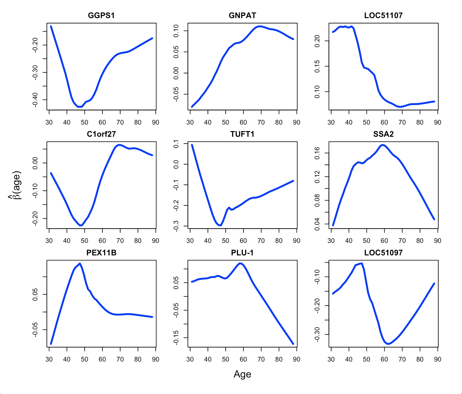
Figure 1: The estimated coefficient functions of the selected nine genes.

4. A Brief Discussion

In this paper, we utilize the conditional correlation between predictors and the empirical distribution function of response given exposure variables to develop a model-free sure independence screening procedure C-SIRS. It is resistant to the heavy-tailed distribution, outliers and extreme values of the response. In addition, C-SIRS is applicable for any model involving exposure variables, including generalized varying coefficient model, and any nonlinear dependent structure. It is also powerful to detect those variables with significant effects on variance components. The ranking consistency and sure screening property of C-SIRS are rendered in both theoretical properties and simulation studies. The breast cancer dataset is systematically analyzed by C-SIRS, along with the comparison with other related methods.

Appendix: Proof of Theorems

Appendix A: Proof of Theorem 1

For easy presentation, we introduce some notations first. $\lambda_{\max}({\bf C})$ and $\lambda_{\min}({\bf C})$ denote the largest and smallest eigenvalues of a matrix ${\bf C}$, respectively. We denote ${\bf v}{\bf v}^{{}^{\mbox{\tiny{T}}}}$ by ${\bf v}^{2}$ for a vector ${\bf v}$ and $\Omega_{\mathcal{A}}(u,y)\stackrel{{\scriptstyle\mbox{{\rm\tiny def}}}}{{=}}\mbox{\rm corr}\{{\bf x}_{\mathcal{A}},I(Y\leq y)\mid u\}$. If we say that $a_{n}-b_{n}$ uniformly in $n$, then it means $\liminf\limits_{n\longrightarrow\infty}{a(n)-b(n)}>0$.

Without loss of generality, we assume that $E(X_{k}\mid u)=0$, $\mbox{\rm var}(X_{k}\mid u)=1$ for $k=1,\cdots,p$ and $\mbox{\rm var}\{I(Y\leq y)\mid u\}=1$. Meanwhile, $\mbox{\boldmath$\beta$}_{\mathcal{A}}(u)$ satisfies $\mbox{\boldmath$\beta$}^{{}^{\mbox{\tiny{T}}}}_{\mathcal{A}}(u)\mbox{\rm cov}({\bf x}_{\mathcal{A}}\mid u)\mbox{\boldmath$\beta$}_{\mathcal{A}}(u)=1$. Then the conditional linearity condition (A1) is simplified as $E\{X_{k}\mid{\bf x}_{\mathcal{A}}^{{}^{\mbox{\tiny{T}}}}\mbox{\boldmath$\beta$}_{\mathcal{A}}(u),u\}=\mbox{\rm cov}\{X_{k},{\bf x}_{\mathcal{A}}^{{}^{\mbox{\tiny{T}}}}\mbox{\boldmath$\beta$}_{\mathcal{A}}(u)\mid u\}\mbox{\boldmath$\beta$}^{{}^{\mbox{\tiny{T}}}}_{\mathcal{A}}(u){\bf x}_{\mathcal{A}}$. Following law of iterated expectations,

$$E\left\{X_{k}I(Y\leq y)\mid u,y\right\}=E\left[E\left\{X_{k}I(Y\leq y)\mid\mbox{\boldmath$\beta$}^{{}^{\mbox{\tiny{T}}}}_{\mathcal{A}}(u){\bf x}_{\mathcal{A}},u,y\right\}\mid u,y\right]$$

$$=E\left[E\left\{X_{k}\mid\mbox{\boldmath$\beta$}^{{}^{\mbox{\tiny{T}}}}_{\mathcal{A}}(u){\bf x}_{\mathcal{A}},u\right\}E\left\{I(Y\leq y)\mid\mbox{\boldmath$\beta$}^{{}^{\mbox{\tiny{T}}}}_{\mathcal{A}}(u){\bf x}_{\mathcal{A}},u,y\right\}\mid u,y\right]$$ (4.1)

$$=\mbox{\rm cov}\left\{X_{k},{\bf x}_{\mathcal{A}}^{{}^{\mbox{\tiny{T}}}}\mbox{\boldmath$\beta$}_{\mathcal{A}}(u)\mid u\right\}E\left\{\mbox{\boldmath$\beta$}^{{}^{\mbox{\tiny{T}}}}_{\mathcal{A}}(u){\bf x}_{\mathcal{A}}I(Y<y)\mid u,y\right\},$$ (4.2)

where (4.1) holds because of the conditional independence of ${\bf x}$ and $Y$ given $\mbox{\boldmath$\beta$}^{{}^{\mbox{\tiny{T}}}}_{\mathcal{A}}(u){\bf x}_{\mathcal{A}}$ and $u$ in (A3) and (4.2) is due to the simplified conditional linearity condition.

$$\max_{k\in\mathcal{A}^{c}}\ \Omega_{k}^{2}(u,y)=\max_{k\in\mathcal{A}^{c}}E^{2}\left\{X_{k}I(Y\leq y)\mid u,y\right\}$$

$$=\max_{k\in\mathcal{A}^{c}}\left[\mbox{\rm cov}^{2}\left\{X_{k},{\bf x}_{\mathcal{A}}^{{}^{\mbox{\tiny{T}}}}\mbox{\boldmath$\beta$}_{\mathcal{A}}(u)\mid u\right\}\right]\cdot E^{2}\left\{\mbox{\boldmath$\beta$}^{{}^{\mbox{\tiny{T}}}}_{\mathcal{A}}(u){\bf x}_{\mathcal{A}}I(Y\leq y)\mid u,y\right\}.$$ (4.3)

Then we start to deal with the first term of (4.3).

$$\max_{k\in\mathcal{A}^{c}}\left[\mbox{\rm cov}^{2}\left\{X_{k},{\bf x}_{\mathcal{A}}^{{}^{\mbox{\tiny{T}}}}\mbox{\boldmath$\beta$}_{\mathcal{A}}(u)\mid u\right\}\right]$$

$$= \mbox{\boldmath$\beta$}^{{}^{\mbox{\tiny{T}}}}_{\mathcal{A}}(u)\left[\max_{k\in\mathcal{A}^{c}}\left\{\mbox{\rm cov}\left({\bf x}_{\mathcal{A}},X_{k}\mid u\right)\mbox{\rm cov}(X_{k},{\bf x}_{\mathcal{A}}^{{}^{\mbox{\tiny{T}}}}\mid u)\right\}\right]\mbox{\boldmath$\beta$}_{\mathcal{A}}(u)$$

$$\leq \mbox{\boldmath$\beta$}^{{}^{\mbox{\tiny{T}}}}_{\mathcal{A}}(u)\mbox{\rm cov}({\bf x}_{\mathcal{A}},{\bf x}_{\mathcal{A}^{c}}^{{}^{\mbox{\tiny{T}}}}\mid u)\mbox{\rm cov}({\bf x}_{\mathcal{A}^{c}},{\bf x}_{\mathcal{A}}^{{}^{\mbox{\tiny{T}}}}\mid u)\mbox{\boldmath$\beta$}_{\mathcal{A}}(u)$$

$$= \{\mbox{\boldmath$\beta$}^{{}^{\mbox{\tiny{T}}}}_{\mathcal{A}}(u)\mbox{\rm cov}^{1/2}({\bf x}_{\mathcal{A}},{\bf x}_{\mathcal{A}}^{{}^{\mbox{\tiny{T}}}}\mid u)\}\mbox{\rm cov}^{-1/2}({\bf x}_{\mathcal{A}},{\bf x}_{\mathcal{A}}^{{}^{\mbox{\tiny{T}}}}\mid u)\mbox{\rm cov}({\bf x}_{\mathcal{A}},{\bf x}_{\mathcal{A}^{c}}^{{}^{\mbox{\tiny{T}}}}\mid u)$$

$$\cdot\mbox{\rm cov}({\bf x}_{\mathcal{A}^{c}},{\bf x}_{\mathcal{A}}^{{}^{\mbox{\tiny{T}}}}\mid u)\mbox{\rm cov}^{-1/2}({\bf x}_{\mathcal{A}},{\bf x}_{\mathcal{A}}^{{}^{\mbox{\tiny{T}}}}\mid u)\left\{\mbox{\rm cov}^{1/2}({\bf x}_{\mathcal{A}},{\bf x}_{\mathcal{A}}^{{}^{\mbox{\tiny{T}}}}\mid u)\mbox{\boldmath$\beta$}_{\mathcal{A}}(u)\right\}$$

$$\leq \lambda_{\max}\left\{\mbox{\rm cov}^{-1/2}({\bf x}_{\mathcal{A}},{\bf x}_{\mathcal{A}}^{{}^{\mbox{\tiny{T}}}}\mid u)\mbox{\rm cov}({\bf x}_{\mathcal{A}},{\bf x}_{\mathcal{A}^{c}}^{{}^{\mbox{\tiny{T}}}}\mid u)\mbox{\rm cov}({\bf x}_{\mathcal{A}^{c}},{\bf x}_{\mathcal{A}}^{{}^{\mbox{\tiny{T}}}}\mid u)\mbox{\rm cov}^{-1/2}({\bf x}_{\mathcal{A}},{\bf x}_{\mathcal{A}}^{{}^{\mbox{\tiny{T}}}}\mid u)\right\}$$

$$\leq \lambda_{\max}\left\{\mbox{\rm cov}({\bf x}_{\mathcal{A}},{\bf x}_{\mathcal{A}^{c}}^{{}^{\mbox{\tiny{T}}}}\mid u)\mbox{\rm cov}({\bf x}_{\mathcal{A}^{c}},{\bf x}_{\mathcal{A}}^{{}^{\mbox{\tiny{T}}}}\mid u)\right\}\cdot\lambda_{\max}\left\{\mbox{\rm cov}^{-1}({\bf x}_{\mathcal{A}},{\bf x}_{\mathcal{A}}^{{}^{\mbox{\tiny{T}}}}\mid u)\right\}$$

$$= \lambda_{\max}\left\{\mbox{\rm cov}({\bf x}_{\mathcal{A}},{\bf x}_{\mathcal{A}^{c}}^{{}^{\mbox{\tiny{T}}}}\mid u)\mbox{\rm cov}({\bf x}_{\mathcal{A}^{c}},{\bf x}_{\mathcal{A}}^{{}^{\mbox{\tiny{T}}}}\mid u)\right\}/\lambda_{\min}\left\{\mbox{\rm cov}({\bf x}_{\mathcal{A}},{\bf x}_{\mathcal{A}}^{{}^{\mbox{\tiny{T}}}}\mid u)\right\},$$

where (S4.Ex9) holds because of the fact $\lambda_{\max}({\bf C}^{{}^{\mbox{\tiny{T}}}}{\bf B}{\bf C})\leq\lambda_{\max}({\bf B})\lambda_{\max}({\bf C}^{{}^{\mbox{\tiny{T}}}}{\bf C})$, where the matrix ${\bf B}\geq 0$. Similarly, we can verify that

$$E^{2}\left\{\mbox{\boldmath$\beta$}^{{}^{\mbox{\tiny{T}}}}_{\mathcal{A}}(u){\bf x}_{\mathcal{A}}I(Y\leq y)\mid u,y\right\}\leq\lambda_{\max}\left[E^{2}\left\{{\bf x}_{\mathcal{A}}I(Y\leq y)\mid u,y\right\}\right]/\lambda_{\min}\left\{\mbox{\rm cov}({\bf x}_{\mathcal{A}},{\bf x}_{\mathcal{A}}^{{}^{\mbox{\tiny{T}}}}\mid u)\right\}.$$

These two inequations yield that

$$\max_{k\in\mathcal{A}^{c}}\omega_{k}=\max_{k\in\mathcal{A}^{c}}E\{\Omega_{k}^{2}(y,u)\}\leq E\{\max_{k\in\mathcal{A}^{c}}\ \Omega_{k}^{2}(y,u)\}$$

$$\leq E\left[\lambda_{\max}\left\{\mbox{\rm cov}({\bf x}_{\mathcal{A}},{\bf x}_{\mathcal{A}^{c}}^{{}^{\mbox{\tiny{T}}}}\mid u)\mbox{\rm cov}({\bf x}_{\mathcal{A}^{c}},{\bf x}_{\mathcal{A}}^{{}^{\mbox{\tiny{T}}}}\mid u)\right\}\lambda_{\max}\{\Omega_{\mathcal{A}}^{2}(y,u)\}/\lambda^{2}_{\min}\left\{\mbox{\rm cov}({\bf x}_{\mathcal{A}},{\bf x}_{\mathcal{A}}^{{}^{\mbox{\tiny{T}}}}\mid u)\right\}\right],$$

which completes the proof.

Appendix B: Proof of Theorem 2

Define $E(\cdot\mid u)=g(\cdot\mid u)/f(u)$, and

$$\widehat{E}(X_{k}\mid u)=\widehat{g}(X_{k}\mid u)/\widehat{f}(u),\ \widehat{E}\{I(Y\leq y)\mid u\}=\widehat{g}(y\mid u)/\widehat{f}(u),$$

where $\widehat{g}(X_{k}\mid u)\stackrel{{\scriptstyle\mbox{{\rm\tiny def}}}}{{=}}n^{-1}\sum_{i=1}^{n}K_{h}(u_{i}-u)X_{ik}$, $\widehat{g}(y\mid u)\stackrel{{\scriptstyle\mbox{{\rm\tiny def}}}}{{=}}n^{-1}\sum_{i=1}^{n}K_{h}(u_{i}-u)I(Y_{i}\leq y)$, $\widehat{f}(u)\stackrel{{\scriptstyle\mbox{{\rm\tiny def}}}}{{=}}n^{-1}\sum_{i=1}^{n}K_{h}(u_{i}-u)$ and $K_{h}(u)=K(u/h)/h$.

Lemma 1.

(Hoeffding’s Inequality (Hoeffding,, 1963)) Let $X_{1},\ldots,X_{n}$ be independent random variables, and $\mbox{Pr}(a_{i}\leq X_{i}\leq b_{i})=1$ for $i=1,\ldots,n$. Then

$$\mbox{Pr}\left\{|\overline{X}-E(\overline{X})|\geq t\right\}\leq 2\exp\left\{-2n^{2}t^{2}\Big{/}\sum_{i=1}^{n}(b_{i}-a_{i})^{2}\right\},\textrm{ for any $t>0$. }$$

Lemma 2.

(Liu et al.,, 2014) Suppose that $X$ is a random variable with $E(e^{a|X|})<\infty$ for some $a>0$. Then for any $M>0$, there exist positive constants $b$ and $c$ such that

$$\mbox{Pr}(|X|\geq M)\leq b\exp(-cM).$$

The following lemma is a sight modified version of Theorem 3.1 of Zhu (1993) and Lemma 3.2 of Zhu and Fang, (1996).

Lemma 3.

Suppose that conditions (C1) to (C5) are fulfilled, and $\sup\limits_{\bf x}|X_{k}|\leq M$, then for any $\varepsilon_{n}>0$,

$$\mbox{Pr}\left\{\sup_{u}\left|\widehat{g}(X_{k}\mid u)-E\widehat{g}(X_{k}\mid u)\right|\geq 8MM_{K}h^{-1}n^{-1/2}\varepsilon_{n}\right\}$$

$$\leq 3c\big{(}n^{1/2}/\varepsilon_{n}\big{)}^{4}\exp\left(-\varepsilon_{n}^{2}/128\delta^{2}\right)+4c\delta^{-8}\exp\left(-n\delta^{2}\right),$$

where $\delta\geq\sup\limits_{u}\left[\mbox{\rm var}\left\{K\left(\frac{\widetilde{u}-u}{h}\right)\right\}\right]^{1/2}$.

Lemma 4.

Suppose that conditions (C1) to (C5) are fulfilled, for any $0<\gamma+\theta<1/4$ and $0<\gamma\leq m\theta$, then we have

$$\mbox{Pr}\left\{\sup_{u}\left|\widehat{g}(X_{k}\mid u)-g(X_{k}\mid u)\right|\geq cn^{-\gamma}\right\}\leq a_{1}n^{2}\exp(-b_{1}n^{1/2-2\theta-2\gamma}),$$

where $a_{1}$, $b_{1}$ and $c$ are some positive constants.

Proof of Lemma 4: For any $M>0$,

$$\mbox{Pr}\left\{\sup\limits_{u}\left|\widehat{g}(X_{k}\mid u)-g(X_{k}\mid u)\right|\geq cn^{-\gamma}\right\}$$

$$=\mbox{Pr}\left\{\sup\limits_{u}\left|\widehat{g}(X_{k}\mid u)-g(X_{k}\mid u)\right|\geq cn^{-\gamma},\max|X_{ik}|\leq M\right\}$$

$$+\mbox{Pr}\left\{\sup\limits_{u}\left|\widehat{g}(X_{k}\mid u)-g(X_{k}\mid u)\right|\geq cn^{-\gamma},\max|X_{ik}|\geq M\right\}$$

$$\leq\mbox{Pr}\left\{\sup\limits_{u}\left|\widehat{g}(X_{k}\mid u)-g(X_{k}\mid u)\right|\geq cn^{-\gamma},\max|X_{ik}|\leq M\right\}$$

$$+\mbox{Pr}\left\{\max|X_{ik}|\geq M\ \textrm{for some}\ i\right\}=P_{1}(u)+P_{2},$$

where $P_{1}(u)$ and $P_{2}$ are defined in the obvious way. We derive the first term $P_{1}(u)$. The following arguments are all under the condition $\max|X_{ik}|\leq M$, which is omitted for notation simplicity. We expand $g(X_{k}\mid u)$ in a Taylor series with the Lagrange remainder term under Condition (C3). There exists a positive constant $c_{1}$ such that

$$\sup\limits_{u}\left|E\widehat{g}(X_{k}\mid u)-g(X_{k}\mid u)\right|=\sup\limits_{u}\left|\int K_{h}\left(\widetilde{u}-u\right)\{E(X_{k}\mid\widetilde{u})f(\widetilde{u})-E(X_{k}\mid u)f(u)\}d\widetilde{u}\right|$$

$$=\sup\limits_{u}\left|\int K(t)\{E(X_{k}\mid u+ht)f(u+ht)-E(X_{k}\mid u)f(u)\}\ dt\right|\leq c_{1}\nu_{m}h^{m}.$$

Since the kernel function $K$ is uniformly continuous on its compact support, we have

$$\sup\limits_{u}\left[\mbox{\rm var}\left\{K\left(\frac{\widetilde{u}-u}{h}\right)\right\}\right]^{1/2}\leq\sup\limits_{u}\left\{\int K^{2}\left(\frac{\widetilde{u}-u}{h}\right)f(\widetilde{u})d\widetilde{u}\right\}^{1/2}\leq M_{K}$$

Following the Lemma 3, for $0<\gamma\leq m\theta$,

$$\mbox{Pr}\left\{\sup_{u}\left|\widehat{g}(X_{k}\mid u)-g(X_{k}\mid u)\right|\geq cn^{-\gamma},\max|X_{ik}|\leq M\right\}$$

$$=\mbox{Pr}\left\{\sup_{u}\big{|}\widehat{g}(X_{k}\mid u)-E\widehat{g}(X_{k}\mid u)+E\widehat{g}(X_{k}\mid u)-g(X_{k}\mid u)\big{|}\geq cn^{-\gamma},\max|X_{ik}|\leq M\right\}$$

$$\leq\mbox{Pr}\left\{\sup_{u}\big{|}\widehat{g}(X_{k}\mid u)-E\widehat{g}(X_{k}\mid u)\big{|}\geq cn^{-\gamma}/2,\max|X_{ik}|\leq M\right\}$$

$$=O\left\{n^{2}\exp(-b_{1}n^{1-2\theta-2\gamma}/M^{2})\right\},$$ (4.5)

for some positive constant $b_{1}$.

Then we deal with $\mbox{Pr}\left\{\max|X_{ik}|\geq M\ \textrm{for some}\ i\right\}$. Following the assumption (C5) and Lemma 2, there exist some positive constants $t_{1}$ and $t_{2}$ such that for any $M>0$, $\mbox{Pr}(|X_{k}|\geq M)\leq t_{1}\exp(-t_{2}M)$. Then,

$$\mbox{Pr}\left\{\max|X_{ik}|\geq M\ \textrm{for some}\ i\right\}\leq n\mbox{Pr}(|X_{k}|\geq M)\leq nt_{1}\exp(-t_{2}M)$$

Thus, together with (4.5), we have

$$\mbox{Pr}\left\{\sup\limits_{u}\left|\widehat{g}(X_{k}\mid u)-g(X_{k}\mid u)\right|\geq cn^{-\gamma}\right\}\leq c_{1}n^{2}\exp(-b_{1}n^{1-2\theta-2\gamma}/M^{2})+nt_{1}\exp(-t_{2}M)$$

$$\leq c_{1}n^{2}\exp\{-b_{1}n^{1/2-2\theta-2\gamma}\cdot(n^{1/2}/M^{2})\}+nt_{1}\exp\{-t_{2}n^{1/2-2\theta-2\gamma}\cdot Mn^{2\theta+2\gamma-1/2}\}$$ (4.6)

Following Liu et al., (2014), we take $M=O(n^{\tau})$, where $1/2-2\theta-2\gamma<\tau<1/4$. For large $n$, we can see that $n^{1/2}/M^{2}=n^{1/2-2\tau}>1,\ \textrm{and}\ Mn^{2\theta+2\gamma-1/2}=n^{\tau+2\theta+2\gamma-1/2}>1$. Now (4.6) becomes

$$\mbox{Pr}\left\{\sup\limits_{u}\left|\widehat{g}(X_{k}\mid u)-g(X_{k}\mid u)\right|\geq cn^{-\gamma}\right\}\leq a_{1}n^{2}\exp(-b_{1}n^{1/2-2\theta-2\gamma}),$$

where $a_{1}$, $b_{1}$ and $c$ are some positive constants. The proof is complete.

Lemma 5.

Suppose that conditions (C1) to (C5) are fulfilled, for any $0<\gamma+\theta<1/2$ and $0<\gamma\leq m\theta$, then we have

$$\mbox{Pr}\left\{\sup_{u}\left|\widehat{f}(u)-f(u)\right|\geq cn^{-\gamma}\right\}\leq a_{2}n^{2}\exp(-b_{2}n^{1-2\theta-2\gamma}),$$

$$\mbox{Pr}\left\{\sup_{u,y}\left|\widehat{g}(y\mid u)-g(y\mid u)\right|\geq cn^{-\gamma}\right\}\leq a_{3}n^{3}\exp(-b_{3}n^{1-2\theta-2\gamma}),$$

where $a_{2}$, $b_{2}$, $a_{3}$, $b_{3}$ and $c$ are some positive constants.

Proof of Lemma 5: We use the same technique as the proof for Lemma 4. According to Theorem 3.1 of Zhu (1993) and Lemma 3.1 of Zhu and Fang, (1996), for any $\varepsilon_{n}>0$,

$$\mbox{Pr}\left\{\sup_{u}\left|\widehat{f}(u)-E\widehat{f}(u)\right|\geq 8M_{K}h^{-1}n^{-1/2}\varepsilon_{n}\right\}$$

$$\leq 3A\big{(}n^{1/2}/\varepsilon_{n}\big{)}^{4}\exp\left(-\varepsilon_{n}^{2}/128\delta_{1}^{2}\right)+4A\delta_{1}^{-8}\exp\left(-n\delta_{1}^{2}\right),$$ (4.7)

$$\mbox{Pr}\left\{\sup_{u,y}\left|\widehat{g}(y\mid u)-E\widehat{g}(y\mid u)\right|\geq 8M_{K}h^{-1}n^{-1/2}\varepsilon_{n}\right\}$$

$$\leq 3A\big{(}n^{1/2}/\varepsilon_{n}\big{)}^{6}\exp\left(-\varepsilon_{n}^{2}/128\delta_{2}^{2}\right)+4A\delta_{2}^{-12}\exp\left(-n\delta_{2}^{2}\right),$$ (4.8)

where $\delta_{1}\geq\sup\limits_{u}\left[\mbox{\rm var}\left\{K\left(\frac{\widetilde{u}-u}{h}\right)\right\}\right]^{1/2}$ and $\delta_{2}\geq\sup\limits_{u,y}\left[\mbox{\rm var}\left\{K\left(\frac{\widetilde{u}-u}{h}\right)I(Y\leq y)\right\}\right]^{1/2}$. And $A$ is a generic constant and may take different values at different places. We expand $f(u)$ and $g(y\mid u)$ in a Taylor series with the Lagrange remainder term under Condition (C3). There exists some positive constants $c_{2}$ and $c_{3}$ such that

$$\sup\limits_{u}\left|E\widehat{f}(u)-f(u)\right|=\sup\limits_{u}\left|\int K_{h}\left(\widetilde{u}-u\right)\left\{f(\widetilde{u})-f(u)\right\}d\widetilde{u}\right|$$

$$=\sup\limits_{u}\left|\int K\left(t\right)\{f(u+ht)-f(u)\}\ dt\right|\leq c_{2}\nu_{m}h^{m},$$

$$\sup\limits_{u,y}\left|E\widehat{g}(y\mid u)-g(y\mid u)\right|=\sup\limits_{u}\left|\int K_{h}\left(\widetilde{u}-u\right)\{F(y\mid\widetilde{u})f(\widetilde{u})-F(y\mid u)f(u)\}d\widetilde{u}\right|$$

$$=\sup\limits_{u,y}\left|\int K(t)\{F(y\mid u+ht)f(u+ht)-F(y\mid u)f(u)\}\ dt\right|\leq c_{3}\nu_{m}h^{m}.$$

Since the kernel function $K$ is uniformly continuous on its compact support, we have

$$\sup\limits_{u,y}\left[\mbox{\rm var}\left\{K\left(\frac{\widetilde{u}-u}{h}\right)I(Y\leq y)\right\}\right]^{1/2}\leq\sup\limits_{u}\left\{\int K^{2}\left(\frac{\widetilde{u}-u}{h}\right)f(\widetilde{u})d\widetilde{u}\right\}^{1/2}\leq M_{K}$$

Thus for $0<\gamma\leq m\theta$,

$$\mbox{Pr}\left\{\sup_{u}\left|\widehat{f}(u)-f(u)\right|\geq cn^{-\gamma}\right\}=\mbox{Pr}\left\{\sup_{u}\left|\widehat{f}(u)-E\widehat{f}(u)+E\widehat{f}(u)-f(u)\right|\geq cn^{-\gamma}\right\}$$

$$\leq\mbox{Pr}\left\{\sup_{u}\left|\widehat{f}(u)-E\widehat{f}(u)\right|\geq cn^{-\gamma}/2\right\}=O\left\{n^{2}\exp(-b_{2}n^{1-2\theta-2\gamma})\right\},$$ (4.9)

$$\mbox{Pr}\left\{\sup_{u,y}\left|\widehat{g}(y\mid u)-g(y\mid u)\right|\geq cn^{-\gamma}\right\}=\mbox{Pr}\left\{\sup_{u,y}\big{|}\widehat{g}(y\mid u)-E\widehat{g}(y\mid u)+E\widehat{g}(y\mid u)\right.$$

$$\left.-g(y\mid u)\big{|}\geq cn^{-\gamma}\right\}\leq\mbox{Pr}\left\{\sup_{u,y}\big{|}\widehat{g}(y\mid u)-E\widehat{g}(y\mid u)\big{|}\geq cn^{-\gamma}/2\right\}$$

$$=O\left\{n^{3}\exp(-b_{3}n^{1-2\theta-2\gamma})\right\},$$ (4.10)

where $b_{2}$, $b_{3}$ and $c$ are some positive constants. The proof is complete.

Lemma 6.

(Liu et al.,, 2014) Suppose $T(u,y)$ and $S(u,y)$ are two uniformly-bounded functions of $u$ and $y$. For any given $u$ and $y$, $\widehat{T}(u,y)$ and $\widehat{S}(u,y)$ are estimates of $T(u,y)$ and $S(u,y)$ based on a sample with size $n$. For any $0<\gamma+\theta<1/4$ and $0<\gamma\leq m\theta$, suppose that

$$\mbox{Pr}\left\{\sup_{u,y}\left|\widehat{T}(u,y)-T(u,y)\right|\geq cn^{-\gamma}\right\}\leq a_{4}n^{3}\exp(-b_{4}n^{1/2-2\theta-2\gamma}),$$

$$\mbox{Pr}\left\{\sup_{u,y}\left|\widehat{S}(u,y)-S(u,y)\right|\geq cn^{-\gamma}\right\}\leq a_{5}n^{3}\exp(-b_{5}n^{1/2-2\theta-2\gamma}).$$

where $a_{4}$, $b_{4}$, $a_{5}$, $b_{5}$ and $c$ are some positive constants.Then we have

$$\mbox{Pr}\left\{\sup_{u,y}\left|\widehat{T}(u,y)\widehat{S}(u,y)-T(u,y)S(u,y)\right|\geq cn^{-\gamma}\right\}\leq a_{6}n^{3}\exp(-b_{6}n^{1/2-2\theta-2\gamma}),$$

$$\mbox{Pr}\left\{\sup_{u,y}\left|\widehat{T}(u,y)/\widehat{S}(u,y)-T(u,y)/S(u,y)\right|\geq cn^{-\gamma}\right\}\leq a_{7}n^{3}\exp(-b_{7}n^{1/2-2\theta-2\gamma}),$$

$$\mbox{Pr}\left\{\sup_{u,y}\left|\{\widehat{T}(u,y)\widehat{S}(u,y)\}-\{T(u,y)-S(u,y)\}\right|\geq cn^{-\gamma}\right\}\leq a_{8}n^{3}\exp(-b_{8}n^{1/2-2\theta-2\gamma}),$$

where $a_{i}$, $b_{i}$ for $i=6,7,8$ and $c$ are some positive constants.

Proof of Theorem 2: We divide the proof into two steps.
Step 1. We first prove that, under conditions (C1)-(C5), for any $0<\gamma+\theta\leq 1/4$ and $0<\gamma\leq m\theta$, there exists some positive constant $c$ such that

$$\mbox{Pr}\left(|\widehat{\omega}_{k}-\omega_{k}|\geq cn^{-\gamma}\right)\leq cn^{3}\exp(-cn^{1/2-2\gamma-2\theta}).$$

We define $\Delta_{1}$ and $\Delta_{2}$ as follows,

$$\Delta_{1} = n^{-2}\sum_{i=1}^{n}\sum_{j=1}^{n}\left[\widehat{}\mbox{\rm corr}^{2}\{X_{k},I(Y\leq Y_{j})\mid u_{i}\}-\mbox{\rm corr}^{2}\{X_{k},I(Y\leq Y_{j})\mid u_{i}\}\right];$$

$$\Delta_{2} = n^{-2}\sum_{i=1}^{n}\sum_{j=1}^{n}\left[\mbox{\rm corr}^{2}\{X_{k},I(Y\leq Y_{j})\mid u_{i}\}-\omega_{k}\right].$$

Then we have $\mbox{Pr}\left(|\widehat{\omega}_{k}-\omega_{k}|\geq cn^{-\gamma}\right)\leq\mbox{Pr}\left(|\Delta_{1}|\geq cn^{-\gamma}/2\right)+\mbox{Pr}\left(|\Delta_{2}|\geq cn^{-\gamma}/2\right)$. We deal with the first part of the summation.

$$\mbox{Pr}\left(|\Delta_{1}|\geq cn^{-\gamma}/2\right)\leq\mbox{Pr}\Big{(}n^{-2}\sum_{i=1}^{n}\sum_{j=1}^{n}\left|\widehat{}\mbox{\rm corr}^{2}\{X_{k},I(Y\leq Y_{j})\mid u_{i}\}\right.-$$

$$\left.\mbox{\rm corr}^{2}\{X_{k},I(Y\leq Y_{j})\mid u_{i}\}\right|\geq cn^{-\gamma}/2\Big{)}\leq\mbox{Pr}\Big{(}\sup_{u,y}\left|\widehat{}\mbox{\rm corr}^{2}\{X_{k},I(Y\leq y)\mid u\}\right.-$$

$$\left.\mbox{\rm corr}^{2}\{X_{k},I(Y\leq y)\mid u\}\right|\geq cn^{-\gamma}/2\Big{)}.$$ (4.11)

For notation clarity, we define $\widehat{g}(X_{k},y\mid u)\stackrel{{\scriptstyle\mbox{{\rm\tiny def}}}}{{=}}n^{-1}\sum_{i=1}^{n}K_{h}(u_{i}-u)X_{ik}I(Y_{i}\leq y)$ and $\widehat{g}(X^{2}_{k}\mid u)\stackrel{{\scriptstyle\mbox{{\rm\tiny def}}}}{{=}}n^{-1}\sum_{i=1}^{n}K_{h}(u_{i}-u)X^{2}_{ik}$. Then $\mbox{\rm corr}^{2}\{X_{k},I(Y\leq y)\mid u\}$ can be written as

$$\widehat{}\mbox{\rm corr}^{2}\{X_{k},I(Y\leq y)\mid u\}=\frac{\left\{\widehat{g}(X_{k},y\mid u)\widehat{f}(u)-\widehat{g}(X_{k}\mid u)\widehat{g}(y\mid u)\right\}^{2}}{\left\{\widehat{g}(X_{k}^{2}\mid u)\widehat{f}(u)-\widehat{g}^{2}(X_{k}\mid u)\right\}\left\{\widehat{g}(y\mid u)\widehat{f}(u)-\widehat{g}^{2}(y\mid u)\right\}}$$

Similar to the proof of Lemma 4, we can obtain

$$\mbox{Pr}\left\{\sup_{u}\left|\widehat{g}(X_{k}\mid u)-g(X_{k}\mid u)\right|\geq cn^{-\gamma}\right\}\leq a_{9}n^{2}\exp(-b_{9}n^{1/2-2\gamma-2\theta}),$$

Together with Lemmas 4, 5 and 6, it is clear that

$$\mbox{Pr}\Big{(}\sup\limits_{u,y}\left|\widehat{}\mbox{\rm corr}^{2}\{X_{k},I(Y\leq y)\mid u\}-\mbox{\rm corr}^{2}\{X_{k},I(Y\leq y)\mid u\}\right|\geq cn^{-\gamma}\Big{)}\leq cn^{3}\exp(-cn^{1/2-2\gamma-2\theta}).$$

Thus (4.11) becomes $\mbox{Pr}\left(|\Delta_{1}|\geq cn^{-\gamma}/2\right)\leq cn^{3}\exp(-cn^{1/2-2\gamma-2\theta})$. With Hoeffding’s inequality in Lemma 1, we can show that $\mbox{Pr}\left(|\Delta_{2}|\geq cn^{-\gamma}/2\right)\leq 2\exp(-c^{2}n^{1-2\gamma}/2)$. Thus, there exists some positive constants $c$ such that

$$\mbox{Pr}\left(|\widehat{\omega}_{k}-\omega_{k}|\geq cn^{-\gamma}\right)\leq cn^{3}\exp(-cn^{1/2-2\gamma-2\theta}).$$

Step 2. Assume the condition $\min\limits_{k\in\mathcal{A}}\ \omega_{k}\geq 2cn^{-\gamma}$. We prove that

$$\mbox{Pr}(\cal{A}\subseteq\widehat{\cal{A}}) \geq 1-O\left\{n^{3}|\mathcal{A}|\exp(-cn^{1/2-2\gamma-2\theta})\right\}.$$

If $\mathcal{A}\nsubseteq\widehat{\mathcal{A}}$, there must exist some $j\in\mathcal{A}$ such that $\widehat{\omega}_{j}<cn^{-\gamma}$. Under the condition $\min\limits_{k\in\mathcal{A}}\ \omega_{k}\geq 2cn^{-\gamma}$, we have $\left|\widehat{\omega}_{j}-\omega_{j}\right|\geq cn^{-\gamma}$ for this particular $j$, which implies

$$\{\mathcal{A}\nsubseteq\widehat{\cal{A}}\}\subseteq\{\left|\widehat{\omega}_{j}-\omega_{j}\right|\geq cn^{-\gamma},\,\text{for some }j\in\mathcal{A}\}.$$

Then, it is clear that

$$\mbox{Pr}(\cal{A}\subseteq\widehat{\cal{A}}) \geq 1-\mbox{Pr}\left\{\left|\widehat{\omega}_{j}-\omega_{j}\right|\geq cn^{-\gamma},\,\text{for some }j\in\mathcal{A}\right\}$$

$$\geq 1-|\mathcal{A}|\max_{j\in\mathcal{A}}\mbox{Pr}\{|\widehat{\omega}_{j}-\omega_{j}|\geq cn^{-\gamma}\}$$

$$\geq 1-O\left\{n^{3}|\mathcal{A}|\exp(-cn^{1/2-2\gamma-2\theta})\right\},$$

which implies the desired conclusion.

Appendix C: Proof of Theorem 3

The conditions (A1)-(A3) illustrate that $\min\limits_{k\in\cal{A}}\ \omega_{k}-\max\limits_{k\in\mathcal{A}^{c}}\ \omega_{k}\geq 0$.Thus, there exists some $\delta>0$ such that $\min\limits_{k\in\cal{A}}\ \omega_{k}-\max\limits_{k\in\mathcal{A}^{c}}\ \omega_{k}=\delta$. Then we have

$$\mbox{Pr}\left\{\min\limits_{k\in\cal{A}}\widehat{\omega}_{k}\leq\max\limits_{k\in\mathcal{A}^{c}}\widehat{\omega}_{k}\right\}\leq\mbox{Pr}\left\{\min\limits_{k\in\cal{A}}\widehat{\omega}_{k}-\min\limits_{k\in\cal{A}}\omega_{k}+\delta\leq\max\limits_{k\in\mathcal{A}^{c}}\widehat{\omega}_{k}-\max\limits_{k\in\mathcal{A}^{c}}\omega_{k}\right\}$$

$$\leq\mbox{Pr}\left\{\left|(\min\limits_{k\in\cal{A}}\widehat{\omega}_{k}-\max\limits_{k\in\mathcal{A}^{c}}\widehat{\omega}_{k})-(\min\limits_{k\in\cal{A}}\omega_{k}-\max\limits_{k\in\mathcal{A}^{c}}\omega_{k})\right|\geq\delta\right\}$$

$$\leq\mbox{Pr}\left\{2\max\limits_{1\leq k\leq p}\left|\widehat{\omega}_{k}-\omega_{k}\right|\geq\delta\right\}\leq O\left\{p\,n^{3}\exp\left(-cn^{1/2-2\theta}\right)\right\},$$

Then by Fatou’s Lemma,

$$\mbox{Pr}\left\{\liminf\limits_{n\longrightarrow\infty}\left(\min\limits_{k\in\cal{A}}\widehat{\omega}_{k}-\max\limits_{k\in\mathcal{A}^{c}}\widehat{\omega}_{k}\right)\leq 0\right\}\leq\lim\limits_{n\rightarrow\infty}\mbox{Pr}\left(\min\limits_{k\in\cal{A}}\widehat{\omega}_{k}-\max\limits_{k\in\mathcal{A}^{c}}\widehat{\omega}_{k}\leq 0\right)=0$$

In other words, we have $\mbox{Pr}\left\{\liminf\limits_{n\longrightarrow\infty}\left(\min\limits_{k\in\cal{A}}\widehat{\omega}_{k}-\max\limits_{k\in\mathcal{A}^{c}}\widehat{\omega}_{k}\right)>0\right\}=1.$

References

12006Chin et al., Chin et al., (2006)chin2006genomic Chin, K., DeVries, S., Fridlyand, J., Spellman, P. T., Roydasgupta, R., Kuo, W.-L., Lapuk, A., Neve, R. M., Qian, Z., Ryder, T., et al. (2006). Genomic and transcriptional aberrations linked to breast cancer pathophysiologies. Cancer Cell, 10(6):529–541. 22017DeSantis et al., DeSantis et al., (2017)desantis2017breast DeSantis, C. E., Ma, J., Goding Sauer, A., Newman, L. A., and Jemal, A. (2017). Breast cancer statistics, 2017, racial disparity in mortality by state. CA: A Cancer Journal for Clinicians, 67(6):439–448. 32014Fan et al., Fan et al., (2014)Fan2014Nonparametric Fan, J., Ma, Y., and Dai, W. (2014). Nonparametric independence screening in sparse ultra-high dimensional varying coefficient models. Journal of the American Statistical Association, 109(507):1270–1284. 42011Fan et al., Fan et al., (2011)FanFengSong:2011 Fan, J., Feng, Y., and Song, R. (2011). Nonparametric independence screening in sparse ultra-high dimensional additive models. Journal of the American Statistical Association, 106(494):544–557. 52008Fan and Lv, Fan and Lv, (2008)fan2008sure Fan, J. and Lv, J. (2008). Sure independence screening for ultrahigh dimensional feature space. Journal of the Royal Statistical Society: Series B, 70(5):849–911. 62010Fan and Song, Fan and Song, (2010)fan2010sure Fan, J. and Song, R. (2010). Sure independence screening in generalized linear models with NP-dimensionality. The Annals of Statistics, 38(6):3567–3604. 72013He et al., He et al., (2013)he2013quantile He, X., Wang, L., Hong, H. G. (2013). Quantile-adaptive model-free variable screening for high-dimensional heterogeneous data. The Annals of Statistics, 41(1):342–369. 81963Hoeffding, Hoeffding, (1963)Wassily1963Probability Hoeffding, W. (1963). Probability inequalities for sums of bounded random variables. Journal of the American Statistical Association, 58(301):13–30. 9Li et al., 2012a(9)li2012robust Li, G., Peng, H., Zhang, J., and Zhu, L. (2012a). Robust rank correlation based screening. The Annals of Statistics, 40(3):1846–1877. 10Li et al., 2012b(10)li2012feature Li, R., Zhong, W., and Zhu, L. (2012b). Feature screening via distance correlation learning. Journal of the American Statistical Association, 107(499):1129–1139. 112014Liu et al., Liu et al., (2014)Liu2014Feature Liu, J., Li, R., and Wu, R. (2014). Feature selection for varying coefficient models with ultrahigh dimensional covariates. Journal of the American Statistical Association, 109(505):266–274. 122015Liu et al., Liu et al., (2015)Liu2015Aselective Liu, J., Zhong, W. and Li, R. (2015). A selective overview of feature screening for ultrahigh-dimensional data. Science China Mathematics, 58(10):2033–2054. 132000McPherson et al., McPherson et al., (2000)mcpherson2000abc McPherson, K., Steel, C., and Dixon, J. (2000). Abc of breast diseases: breast cancer epidemiology, risk factors, and genetics. BMJ: British Medical Journal, 321(7261):624-628. 142015Wang et al., Wang et al., (2015)wang2015conditional Wang, X., Pan, W., Hu, W., Tian, Y., and Zhang, H. (2015). Conditional distance correlation. Journal of the American Statistical Association, 110(512):1726–1734. 152018Wen et al., Wen et al., (2018)wen2018sure Wen, C., Pan, W., Huang, M., and Wang, X. (2018). Sure independence screening adjusted for confounding covariates with ultrahigh dimensional data. Statistica Sinica, 28:293–317. 162009Witten et al., Witten et al., (2009)witten2009penalized Witten, D. M., Tibshirani, R., and Hastie, T. (2009). A penalized matrix decomposition, with applications to sparse principal components and canonical correlation analysis. Biostatistics, 10(3):515–534. 17PMA(17)PMA:2013 Witten, D. M., Tibshirani, R., Gross, S. and Narasimhan, B. PMA: Penalized multivariate analysis. R package version 1.0.9, 2013. Available from: http://CRAN.R-project.org/package=PMA. 182011Zhu et al., Zhu et al., (2011)zhu2011model Zhu, L. P., Li, L., Li, R., and Zhu, L. X. (2011). Model-free feature screening for ultrahigh-dimensional data. Journal of the American Statistical Association, 106(496):1464–1475. 191993ZhuZhu (1993)Zhu:1993 Zhu, L. X. (1993). Convergence rates of the empirical processes indexed by the classes of functions with applications. Journal of Systems Science and Mathematical Sciences, 13(1):33–41. 201996Zhu and Fang, Zhu and Fang, (1996)zhu1996Asymptotics Zhu, L. X. and Fang, K. T. (2007). Asymptotics for kernel estimate of sliced inverse regression. The Annals of Statistics, 24(3):1053–1068.