Model-aware Quantile Regression for Discrete Data

Abstract

Quantile regression relates the quantile of the response to a linear predictor. For a discrete response distributions, like the Poission, Binomial and the negative Binomial, this approach is not feasible as the quantile function is not bijective. We argue to use a continuous model-aware interpolation of the quantile function, allowing for proper quantile inference while retaining model interpretation. This approach allows for proper uncertainty quantification and mitigates the issue of quantile crossing. Our reanalysis of hospitalisation data considered in Congdon (2017) shows the advantages of our proposal as well as introducing a novel method to exploit quantile regression in the context of disease mapping.

1 Introduction

Quantile regression is a supervised technique aimed at modelling the quantiles of the conditional distribution of some response variable, introduced by Koenker and Bassett (1978). Mean regression is concerned with modelling conditional expectations, whereas quantile regression is especially useful when the tails of the distribution are of interest, as for example when the focus is on extreme behaviour, or when covariates may not affect the whole population uniformly.

Let $Q_{\alpha}(Y_{i}\mid X_{i})$ be the quantile of level $\alpha$ of the conditional distribution of the $i$th observation $Y_{i}\mid X_{i}$, in a sample of size $n$. Point estimates for quantile regression models of the form

$$Q_{\alpha}(Y_{i}\mid X_{i})=X_{i}^{t}\beta_{\alpha}\quad(i=1,\dots,n)$$ (1)

are typically obtained by minimising the following empirical risk:

$$\widehat{\beta}_{\alpha}=\arg\min_{\beta_{\alpha}}\sum_{i=1}^{n}\rho_{\alpha}(Y_{i}-X_{i}^{t}\beta_{\alpha}.)$$ (2)

Here $\rho_{\alpha}(x)=x(\alpha-\mathbb{I}{\{x<0\}})$, with $\mathbb{I}$ being the indicator function, is known as the check loss function. As the optimisation problem in (2) does not depend on the distribution of the response variable, quantile regression is typically considered a model-free technique. Even likelihood based methods, including Bayesian procedures, for which a model assumption on the dependent variables is needed, do not often exploit the generating distribution of the response variable, but make use of working likelihoods instead. The classical model assumption in quantile regression is that of the response being generated by an Asymmetric Laplace Distribution (Yu and Moyeed, 2001; Yue and Rue, 2011), which, rather than representing an hypothesis on the generating mechanism of the data, is motivated by the fact the resulting Maximum Likelihood estimator coincides with the optimum of (2).

These approaches fail when the response variable is discrete. The Asymmetric Laplace distribution assumption, in fact, implies that the observations are continuous, while in the approach based on the direct optimisation of  (2), inferential procedure beyond point estimations are compromised by the non-differentiability of the objective function, which, together with the points of positive mass of one of the variables involved in the optimisation problem, make it challenging to derive an asymptotic distribution for the sample quantiles (Machado and Santos Silva, 2005). Quantile inference for discrete data cannot thus be carried out directly, but it is necessary to enforce additional smoothing on the response variable, and model a continuous approximation of it instead.

In most of the quantile regression literature, such approximation is obtained by means of jittering, i.e. perturbing the discrete distribution by adding continuous and bounded noise, as first proposed by Machado and Santos Silva (2005). When the noise taken to be an Uniform random variable between $0$ and $1$, jittering can be thought of as an interpolation strategy, as the following one-to- one relationship between the quantiles of the jittered response $Y_{i}\mid X_{i}$ and those of the original variable of interest $Y^{*}_{i}\mid X_{i}$ holds for each observation in the sample:

$$Q_{\alpha}(Y^{*}_{i}\mid X_{i})=\lceil Q_{\alpha}(Y_{i}\mid X_{i})-1\rceil\quad(i=1,\dots,n).$$

Regression models can be specified and fitted for $Q_{\alpha}(Y_{i}\mid X_{i})$, since it is a continuous function, however, the dependence of the distribution of $Y_{i}\mid X_{i}$ on the distribution of the arbitrarily chosen noise variable, may hinder the interpretation of $Q_{\alpha}(Y_{i}\mid X_{i})$ as a continuous version of $Q_{\alpha}(Y^{*}_{i}\mid X_{i})$.

We argue to use a model-aware interpolation strategy for building continuous quantile function to be exploited in quantile regression. Our continuous interpolation is tailored to the true distribution of the discrete response and retains the model interpretation of the discrete counterpart, thus providing a stronger justification to the modelling of the continuous quantiles as a proxy of the discrete ones. Additionally, our interpolation scheme also overcomes two more drawbacks of jittering, namely the fact that the new continuous variable is smooth over the entire support and it does not depend on specific realizations of the noise.

In order to fully exploit the distributional assumptions required for the approximation of discrete response variables, we propose a new approach to quantile regression, based on the direct modelling of the quantiles of the generating distribution; in doing so, we address the lack of generating likelihoods in quantile regression. This proposal allows us to extend the Generalized Linear (Mixed) Model framework to quantile regression by redefining the link function. This formulation not only recast quantile regression in a more cohesive setting and overcomes the fragmentation of quantile regression literature, but it is also key to an efficient and ready to use fitting procedure, as the connection allows to estimate the model using R-INLA (Rue et al., 2009; Lindgren and Rue, 2015; Rue et al., 2017; Bakka et al., 2018; Krainski et al., 2018). We show that by exploiting the response distribution in the fitting procedures, it is possible to mitigate the phenomenon of quantile crossing, to provide a unified framework for quantile regression and to obtain proper uncertainty quantification in Bayesian settings.

2 Model-Based Quantile Regression

As opposed to mean regression, where generalization of the basic linear model heavily rely on the response distribution, in quantile regression, with the noticeable exception of Noufaily and Jones (2013); Opitz et al. (2018); Castro-Camilo et al. (2018), generating models are rarely considered. The likelihood assumption commonly found in quantile regression, the Asymmetric Laplace Distribution, is not motivated by the shape of the data. The use of the Asymmetric Laplace Distribution with respect to a proper model may seem appealing due to the apparently weak modeling assumption on the response. However, adopting the Asymmetric Laplace Distribution imposes several restriction that may not be obvious nor desirable in applications: the skewness of the density is fully determined when a specific percentile is chosen, the density is symmetric when $\alpha=0.5$ and the mode of the error distribution is at $0$ regardless of $\alpha$, which results in rigid error density tails for extreme percentiles (Yan and Kottas, 2017).

The limitations of using a working likelihood are even more critical in the Bayesian framework, where the lack of a generating likelihood implies that the validity of posterior inference is no longer guaranteed by Bayes Theorem. As shown by Yang et al. (2016), the scale parameter of the Asymmetric Laplace Distribution affects the posterior variance, despite not having any impact on the quantile itself, and although they provide a corrected adjusted variance, their result is only asymptotically valid.

We reject altogether the use of a working likelihood in favor of the true generating model and we argue to use a model-based quantile regression, which exploits the shape of the conditional distribution to link the covariates of interest to the distribution parameter. This approach is general enough to be adopted in any inferential paradigm, however it is especially appealing in the Bayesian framework since allows for proper uncertainty quantification. Our fitting procedure can be formalized in two steps.

Step1 - Modelling.

Assume that for each unit $i$, $Y_{i}\mid X_{i}$ has a known continuous distribution $F(y_{i};\theta_{i})$, where $\theta_{i}$ is the model parameter, for simplicity $\theta_{i}\in\mathbb{R}$. For each $\alpha$, the quantile of $Y_{i}\mid X_{i}$, $Q_{\alpha}(Y_{i}\mid X_{i})$ is modelled as

$$Q_{\alpha}(Y_{i}\mid X_{i})=g(\eta^{\alpha}_{i})\quad(i=1,\dots,n)$$ (3)

where $g$ is a well behaved link function and $\eta_{i}^{\alpha}$ is the linear predictor, which depends on the level $\alpha$ of the quantile. No restriction needs to be placed on the linear predictor, which can include fixed as well as random effect. Our approach is thus flexible enough to include parametric or semi parametric models, where the interest may lay in assessing the difference in the impact that the covariate may have at different levels of the distribution, as well as fully non parametric models, where the focus is on prediction.

Step 2 - Mapping.

The quantile $Q_{\alpha}(Y_{i}\mid X_{i})$ is mapped to the parameter $\theta_{i}$ as

$$\theta_{i}=h(Q_{\alpha}(Y_{i}\mid X_{i}),\alpha)\quad(i=1,\dots,n)$$ (4)

where the function $h$ must be invertible to ensure the identifiability of the model and explicitly depends on the quantile level $\alpha$. The map $h$ gives us a first interpretation of model-based quantile regression as a reparametrization of the generating likelihood function $F(y_{i};\theta_{i})$, in terms of its quantiles, i.e. $F(y_{i};Q_{\alpha}(Y_{i}\mid X_{i})=h^{-1}(\theta_{i},\alpha))$.

By linking the quantiles of the generating distribution to its parameter $\theta_{i}$, we are indirectly modeling $\theta_{i}$ as well, hence we are implicitly building a connection between quantile regression and Generalized Linear (Mixed) Models. The modeling and mapping steps can be considered as a way to define the link function, in the Generalized Linear Models sense, as the composition $\theta_{i}=h(g(\eta_{i}))$. This allows us to rephrase quantile regression as a new link function in a standard Generalized Linear Models problem. Drawing a path from Generalized Linear Models to quantile regression is instrumental in the fitting however the pairing is only formal: coefficients and random effect retain different interpretations. From a computational standpoint, the main advantage of coupling quantile regression to Generalized Linear Models is that this new class of models can be fitted in standard software packages like R-INLA, which allows for both flexibility in the model definition and efficiency in their fitting. Extensions to the case of multivariate parameters, i.e. $\theta_{i}\in\mathbb{R}^{d}$, with $d>1$, are also possible, and require all the components of the model parameter $\theta_{i}$ to be redefined as a function of the quantiles.

3 Poisson Data

Quantile regression cannot be defined for discrete responses, hence the standard practice is to model a continuous approximation of the quantile function. When such approximation is obtained via mean of jittering as in Machado and Santos Silva (2005), the dependence of the shape of the continuous quantiles on the distribution of the noise variable may hinder the interpretation of the jittered quantile.

Figure 1: Top: c.d.f. of the discrete and continuous Poisson distribution for several values of $\lambda$. Bottom: quantile function of the discrete and continuous Poisson distribution as a function of $\lambda$.

We build the continuous approximation by providing a model-aware strategy, resulting in a stronger justification of the new quantile functions as a continuous version of the discrete ones. Inspired by Ilienko (2013), we focus on random variables satisfying the following assumption, for which the extension to the continuous case is immediate.

Assumption The cumulative distribution of the discrete random variable $X^{*}$ admits the following representation

$$F_{X^{*}}(x;\theta)=k(\lfloor x\rfloor,\theta)$$ (5)

where $k$ is a continuous function in the first argument.

With this assumption, the continuous interpolation can be defined by removing the floor operator, and the function $k(x,\theta)$ is the cumulative distribution function of $X$, a continuous version of $X^{*}$. Note that, for all integer $x$

$$k(\lfloor x\rfloor,\theta)=k(x,\theta).$$ (6)

Incidentally, this way of making variables continuous is well embedded in statistical culture: even the discrete and continuous version of the Uniform distribution are related in a similar manner.

3.1 Continuous Poisson

The class of distribution defined by (5) and (6) is broad enough to include the three discrete distribution most frequently encountered in applications: Poisson, Binomial and Negative Binomial. We explore in detail the Poisson case; the other two are trivial extensions.

We write the cumulative density function for the Poisson as the ratio of Incomplete and Regular Gamma function:

$$X^{*}\sim\text{Poisson}(\lambda)\quad\quad F_{X^{*}}(x)=\frac{\Gamma(\lfloor x\rfloor+1,\lambda)}{\Gamma(\lfloor x\rfloor+1)}\quad x\geq 0$$ (7)

where

$$\Gamma(x,\lambda)=\int_{\lambda}^{\infty}e^{-s}s^{x-1}\text{d}s$$

is the upper incomplete Gamma function. As in Ilienko (2013), extending the Poisson distribution to the continuous case from this formulation is now immediate:

$$X\sim\text{Continuous Poisson}(\lambda)\quad\quad F_{X}(x)=\frac{\Gamma(x+1,\lambda)}{\Gamma(x+1)}\quad x>-1.$$ (8)

where the domain has been extended from $x\geq 0$ to $x>-1$. Following Ilienko (2013), it follows directly that $F_{X}(x)$ is a well defined distribution function, in the sense that it is non-decreasing in $x$, is right-continuous, $F_{X}(-\infty)=0$ and $F_{X}(\infty)=1$. The definition in (8) is similar to that of Ilienko (2013), but it is shifted by $1$.

Lemma 1

Let $X^{*},X$ be respectively a discrete and continuous Poisson random variable, both with parameter $\lambda$, then $X^{*}=\lceil X\rceil$.

From an interpretation point of view, the pairing is strengthened by the fact that the classical result of an Erlang random variable being the waiting time between occurrences of a Poisson homogeneous process, can be extended to the Continuous Poisson case. This can be trivially shown by replacing the Erlang distribution with the Gamma distribution, which are the same distribution with respectively discrete and continuous parameters.

3.2 Quantile Regression for Poisson Data

Quantile regression for Poisson data can be performed by assuming that, conditionally on covariates $X_{i}$, each response $Y^{*}_{i}$ is generated from a Poisson, i.e.

$$Y^{*}_{i}\mid X_{i}\sim\text{Poisson}(\lambda_{i})\quad(i=1,\dots,n).$$ (9)

The modelling and mapping step can then be specified as follows:

Step 1. Modelling: $Q_{\alpha}(Y_{i}\mid X_{i})=\exp\{\eta_{i}^{\alpha}\}\quad(i=1,\dots,n)$

Step 2. Mapping: $\lambda_{i}=\frac{\Gamma^{-1}(Q_{\alpha}(Y_{i}\mid X_{i})^{\alpha}+1,1-\alpha)}{\Gamma(Q_{\alpha}(Y_{i}\mid X_{i})^{\alpha}+1)}\quad(i=1,\dots,n)$

where $Y_{i}\mid X_{i}\sim\text{Continuous Poisson}(\lambda_{i})$. While modelling quantiles of a continuous approximation implies that the fitted quantiles curves are not discrete, as a consequence of Lemma 1, the equivariance property of quantile guarantees that

$$Q_{\alpha}(Y_{i}\mid X_{i})=Q_{\alpha}(\lceil Y^{*}_{i}\rceil\mid X_{i})=\lceil Q_{\alpha}(Y^{*}_{i}\mid X_{i})\rceil\quad(i=1,\dots,n).$$ (10)

3.3 Good Properties - Crossing

One of the most prominent issues in quantile regression literature is that estimated quantile curves may intersect when more than one quantile level is considered. This phenomenon, usually referred to as quantile crossing, which impedes the interpretability of the results, is a consequence of fitting one quantile curve at the time, and may be overcame by jointly estimate multiple quantiles, see for example Bondell et al. (2010). Our proposal can also be extended to the multiple quantile case performing simultaneous estimation by smoothing over quantile levels through a spline model, as in Wei et al. (2012).

However, even in the single quantile case, our method is less affected by this issue by definition, as the presence of a known generating likelihood informs the fitting mechanism on the other quantiles, hence reducing the impact of fitting separate models for each quantile.

Moreover, while in general it is not possible to completely avert the crossing, as it would mean that quantile curves are parallel, intersection can be avoided when the domain of the covariates is bounded.

Lemma 2

Let $Y_{i}^{*}\mid X_{i}$ and $Y_{i}\mid X_{i}$ be distributed respectively as a discrete and continuous Poisson with parameter $\lambda_{i}$, and let $X_{i}\in\mathbb{R}^{+}$. Consider the model $Q_{\alpha}(Y_{i}\mid X_{i})=\exp\{\beta_{\alpha}X_{i}\}$, then the Maximum Likelihood estimator $\hat{\beta_{\alpha}}$ is a non decreasing function of $\alpha$.

The proof is immediate from the equivariance property of Maximum Likelihood estimator and the monotonicity of the exponential function. In the jittering framework, even an apparently restrictive setting as the above can be troublesome. Figure 2 shows the frequency of at least one crossing over $300$ datasets generated from a Poisson random variable $\lambda_{i}=\exp(X_{i})$, where the covariates $X_{i}$ are simulated from the absolute value of a Normal random variable with mean $0$ and standard deviation $1.5$. In this toy example, quantile curves are estimated on an equally spaced grid of $\alpha=(0.05,\dots,0.95)$, using both the jittering approach and our approach. While Lemma 2 holds only asymptotically for a Bayesian estimator of $\beta_{\alpha}$, unless we assume a uniform prior distribution for the coefficient $\beta_{\alpha}$. Figure  2 seems to suggest that the behavior with respect to quantile crossings is good even for small sample sizes.

Figure 2: Frequency of at least one quantile crossing for model-based (solid line) and jittered (dashed line) quantile regression.

4 Continuous Count distributions

The Binomial and the Negative Binomial distribution can be similarly extended to the continuous case. Their cumulative distribution functions can be expressed as:

$$Y^{*}\sim\text{Binomial}(n,p) F_{Y^{*}}(y)=I_{1-p}(n-\lfloor y\rfloor,\lfloor y\rfloor+1)$$ (11)

$$Z^{*}\sim\text{Negative Binomial}(r,p) F_{Z^{*}}(z)=I_{1-p}(r,\lfloor z\rfloor+1)$$ (12)

where $I_{x}(a,b)$ is the regularized incomplete Beta function defined as:

$$I_{x}(a,b)=\frac{\text{B}(a,b,x)}{\text{B}(a,b)} \text{B}(a,b,x)=\int_{x}^{1}t^{a}(1-t)^{b-1}\text{d}t$$ with (13)

The continuous extension is then obtained as:

$$Y\sim\text{Continuous Binomial}(n,p) F_{Y}(y)=I_{1-p}(n-y,y+1)$$ (14)

$$Z\sim\text{Continuous Negative Binomial}(r,p) F_{Z}(z)=I_{1-p}(r,z+1)$$ (15)

These continuous extensions, result in an interpolation of both the cumulative distribution and quantile functions of the discrete counterparts. The advantage of this interpolation scheme is that the behavior of the resulting continuous random variables mimic that of their discrete counterparts. In the discrete case it is well known that the Poisson distribution is the limiting case of both the Binomial and the Negative Binomial and that Binomial and Negative Binomial are entwined in a $1$-to-$1$ relation. Theorem 1 shows how these relationship between variables are preserved in the continuous case, hence the two classes of distribution have similar meaning. From a modeling perspective, in fact, Theorem 1 justifies the interpretation (1) of the Continuous Poisson as an approximation for a Binomial-like distribution in the case of rare events, (2) of the Continuous Negative Binomial as an over-dispersed version of the Continuous Poisson and (3) of the Continuous Negative Binomial as the waiting time until the arrival of the $r$th success in a Binomial-like experiment.

Theorem 1

Let $X$ be a Continuous Poisson random variable with parameter $\lambda$, $Y$ be a Continuous Binomial with parameters $n$ and $p$ and $Z$ be a Continuous Negative Binomial with parameters $r$ and $p$. Then the following relations hold:

1. for $n\rightarrow\infty$ and $p\rightarrow 0$ so that $np\rightarrow\lambda$

   $$F_{Y}(x)=\frac{\text{B}(x+1,N-x,p)}{\text{B}(x+1,N-x)}\longrightarrow\frac{\Gamma(x+1,\lambda)}{\Gamma(x+1)}=F_{X}(x)$$ (16)

2. for $r\rightarrow\infty$ and $p\rightarrow 0$ so that $rp\rightarrow\lambda$ we have

   $$F_{Z}(x)=\frac{\text{B}(x+1,r,p)}{\text{B}(x+1,r)}\longrightarrow\frac{\Gamma(x+1,\lambda)}{\Gamma(x+1)}=F_{X}(x)$$ (17)

3. let $W$ be a Continuous Binomial random variable with parameters $s+r$ and $1-p$, then

   $$F_{Z}(s)=1-F_{W}(r).$$ (18)

5 An application - Disease Mapping

We reanalyse the hospitalisation data of Congdon (2017), described in Table 1. The use of quantile regression instead of mean regression is still relatively unexplored, with exceptions in Congdon (2017) and Chambers et al. (2014). Since the focus of disease mapping is on extreme behaviors of the population, however, quantiles may be a more informative summary than means.

Variable	Description
$Y_{i}$	Counts of emergency hospitalizations for self-harm collected in England over a period of $5$ years (from $2010$ to $2015$). The counts are aggregated over $6791$ are Middle Level Super Output Areas (MSOAs)
$X_{{\tt Depr},i}$	Deprivation, as measured by the 2015 Index of Multiple Deprivation (IMD).
$X_{{\tt SF},i}$	Social fragmentation, measured by a composite index derived from indicators from the 2011 UK Census comprising housing condition and marital status.
$X_{{\tt RS},i}$	Rural status, again measured by a composite indicator aimed at capturing the accessibility to services and facilities such as schools, doctors or public offices.

Table 1: Observed dataset composition

Standard risk measures, such as the ratio between observed and expected cases in each area, the Standardized Mortality (or Morbidity) Ratio (SMR) $SMR_{i}={Y_{i}}/{E_{i}}$, are not reliable here due to the high variability of expected cases $E_{i}$, hence is advisable to introduce a random effect model that stabilizes the risk estimates by borrowing information from the spatial structure of the data. Assuming that, conditionally on covariates $X_{i}=(X_{{\tt Depr},i},X_{{\tt SF},i},X_{{\tt RS},i})$ and random effect $b_{i}$, the observations are generated by a Poisson distribution

$$Y_{i}\mid X_{i},b_{i}\sim\text{Poisson}(\lambda_{i})\quad(i=1,\dots,n)$$ (19)

we adopt the following model for the conditional quantile of level $\alpha$

$${Q}_{\alpha}({Y_{i}\mid X_{i}},b_{i})={E_{i}}\theta^{\alpha}_{i}={E_{i}}\exp\{\eta_{i}\}\quad(i=1,\dots,n).$$ (20)

We opted for a quantile-level approach for handling exposures $E_{i}$ in order to ease interpretation; as we discount each quantile for the exposures, the parameter $\theta_{i}^{\alpha}$ corresponding to the $i^{\tt th}$ area can be considered the relative risk of unit $i$ at level $\alpha$ of the population. More details on the introduction of the exposures $E_{i}$ in the model can be found in Appendix 6.1. The linear predictor $\eta_{i}$ can be decomposed into

$$\eta_{i}=\beta_{0}+\beta_{\tt Depr}{X}_{{\tt Depr},i}+\beta_{\tt SF}{\tt X}_{{\tt SF},i}+\beta_{\tt RS}{\tt X}_{{\tt RS},i}+b_{i}\quad(i=1,\dots,n)$$ (21)

where $\beta_{0}$ represent the overall risk and $b_{i}$ consists in the sum of an unstructured random effect capturing overdispersion and measurement errors and spatially structured random effect. In order to avoid the confounding between the two components of the random effect and to avoid scaling issues we adopt for $b_{i}$ the modified version of the Besag–York–Mollier (BYM) model introduced in Simpson et al. (2017):

$$b_{i}=\frac{1}{\sqrt{\tau_{b}}}\left(\sqrt{1-\phi}v_{i}+\sqrt{\phi}u_{i}\right)\quad(i=1,\dots,n).$$ (22)

Both random effects are normally distributed, and in particular

$$v_{i} \sim N(0,I)\quad(i=1,\dots,n)$$ (23)

$$u_{i} \sim N(0,Q_{u}^{-1})\quad(i=1,\dots,n)$$ (24)

so that $b_{i}\sim N(0,Q_{b}^{-1})$ with $Q_{b}^{-1}=\tau_{b}^{-1}(1-\phi)I+\phi Q_{u}^{-1}$, a weighted sum of the identity matrix ${I}$ and the precision matrix representing the spatial structure $Q_{u}$, scaled in the sense of Sørbye and Rue (2014). We assign priors on the precision $\tau_{b}$ and the mixing parameter $\phi$ using the penalized complexity (PC) approach, as defined in Simpson et al. (2017) and detailed in Riebler et al. (2016) in the special case of disease mapping.

Estimated coefficients shown in Table 2 show that Deprivation has a negative impact, which only slightly attenuates at higher quantile level, meaning that, as we could expect, higher deprivation corresponds to increases in self harm hospitalization. Interestingly, being a rural area seems to have a positive effect instead, with more rural areas being associated to lower rates of hospitalization.

	Mean	1st Quartile	2nd Quartile	3rd Quartile
$\beta_{0}$	-0.598 (0.015)	-0.707 (0.265)	-0.470 (0.275)	-0.512 (0.042)
$\beta_{\tt Depr}$	1.981 (0.031)	2.087 (0.220)	1.960 (0.157)	1.934 (0.059)
$\beta_{\tt RS}$	-0.814 (0.036)	-0.883 (0.127)	-0.878 (0.217)	-0.782 (0.217)
$\beta_{\tt SF}$	0.429 (0.044)	0.562 (0.155)	-0.098 (0.899)	0.399 (0.105)
$\tau_{b}$	6.409 (0.199)	5.768 (0.180)	6.274 (0.196)	7.158 (0.177)
$\phi$	0.838 (0.014)	0.838 (0.014)	0.838 (0.014)	0.817 (0.011)

Table 2: Posterior mean estimates of model parameters (and corresponding standard deviations)

The formulation of the model in terms of relative risk $\theta_{i}^{\alpha}$ as in  (20), is instrumental in detecting areas of immediate concern. We identify the $i$th region as “high risk” if the estimated probability of an increased relative risk for the area is large enough, i.e. if

$$\text{pr}(\hat{\theta}_{i}^{0.25}>1)>t\quad(i=1,\dots,n)$$ (25)

where $t$ is some user-defined threshold, typically $t=0.9$ or $t=0.95$. While the use of exceeedance probabilities for relative risk is common in the disease mapping literature, the benefit of our proposal is to check for increases in the relative risk in the first quartile, which is more worrisome than an increase in the average relative risk. A risk map corresponding to $t=0.95$ is shown in Figure 3. Results are similar to those reported in Congdon (2017), which defines the $i$th area region at “high risk” if $[\hat{\theta}_{i,0.05},\hat{\theta}_{i,0.95}]>1$, thus using only point estimates. With respect to this previous analysis, the use of a model assumption on the response variable allows us to make full use of the posterior distribution, resulting in a more robust interpretation of high risk areas. Additionally, computing exceeedance probabilities strengthens the role of quantile regression in disease mapping.

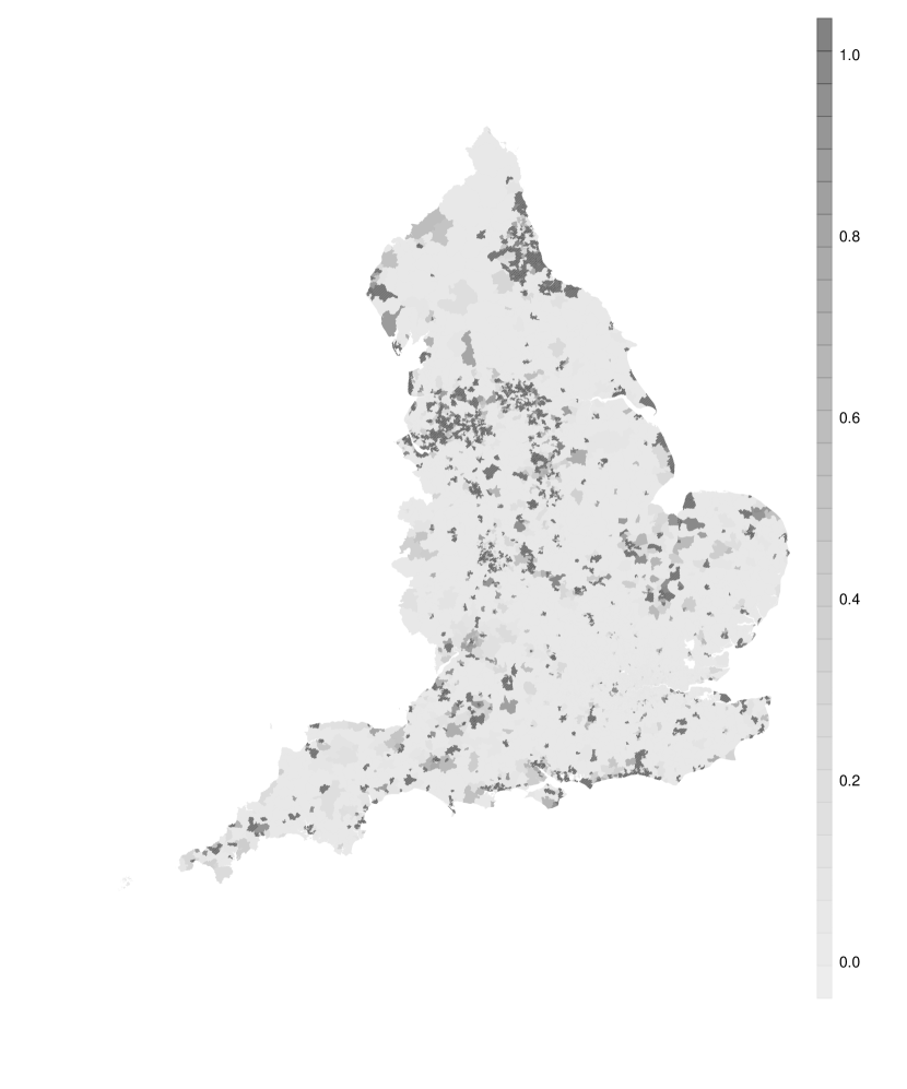
Figure 3: Exceeedance probability for Quantile Relative Risk. Dashed are areas of high risk.

6 Appendix

6.1 Exposures

When count data depend on the size of the unit they have been observed on, it is necessary to rescale them to allow for comparisons. There are two ways of encoding a different observation window $E_{i}$ in the model: by discounting the quantiles directly and considering

$$Q(Y_{i}|X_{i})^{\alpha}/E_{i}\quad(i=1,\dots,n)$$

or by adjusting the global parameter and consider

$$\lambda_{i}/E_{i}\quad(i=1,\dots,n).$$

While in Poisson mean regression these two approaches yield the same results, in Poisson quantile regression they differ. In general

$$\frac{\Gamma^{-1}(E_{i}\exp\{\eta_{i}^{\alpha}\}^{\alpha}+1,1-\alpha)}{\Gamma(E_{i}\exp\{\eta_{i}^{\alpha}\}^{\alpha}+1)}\neq E_{i}\frac{\Gamma^{-1}(\exp\{\eta_{i}^{\alpha}\}^{\alpha}+1,1-\alpha)}{\Gamma(\exp\{\eta_{i}^{\alpha}\}^{\alpha}+1)}\quad(i=1,\dots,n).$$ (26)

A case could be made for both modeling strategies, the former being a “quantile-specific” model while the latter being more of a global model, and choosing between them depends on the application.

6.2 Proof of Lemma 1

By integration by parts we have

$$\frac{\Gamma(x+1,\lambda)}{\Gamma(x+1)}-\frac{\Gamma(x,\lambda)}{\Gamma(x)}=\lambda^{x}e^{\lambda}/\Gamma(x+1)$$ (27)

which is enough to show that:

$$\text{pr}(\lceil X\rceil=x) =\text{pr}(X\in(x-1,x])=F_{X}(x)-F_{X}(x-1)$$

$$=\frac{\Gamma(x+1,\lambda)}{\Gamma(x+1)}-\frac{\Gamma(x,\lambda)}{\Gamma(x)}=\lambda^{x}e^{\lambda}/\Gamma(x+1)$$

$$=\text{pr}(X^{*}=x).$$ (28)

6.3 Proof of Theorem 1

1. immediately follows from Ilienko (2013);

2. follows trivially from (16);

3. follows from

   $$F_{Z}(s) =1-I_{p}(s+1,r)$$

   $$=1-I_{p}((s+r)-(r-1),(r-1)+1)$$

   $$=1-{P}(Y\leq r-1)$$

   $$={P}(Y\geq r).$$ (30)

References

- Bakka et al. (2018) H. Bakka, H. Rue, G. A. Fuglstad, A. Riebler, D. Bolin, J. Illian, E. Krainski, D. Simpson, and F. Lindgren. Spatial modelling with R-INLA: A review. WIREs Computational Statistics, 10:e1443(6), 2018. doi: 10.1002/wics.1443. (Invited extended review).
- Bondell et al. (2010) H. Bondell, A. Krishna, and S. Ghosh. Joint Variable Selection for Fixed and Random Effects in Linear Mixed‐Effects Models. Biometrics, 66(4):1069–1077, 2010. ISSN 0006341X. doi: 10.1111/j.1541-0420.2010.01391.x.Joint. URL http://onlinelibrary.wiley.com/doi/10.1111/j.1541-0420.2010.01391.x/full.
- Castro-Camilo et al. (2018) D. Castro-Camilo, R. Huser, and H. Rue. A three-stage model for short-term extreme wind speed probabilistic forecasting. Journal of Agricultural, Biological, and Environmental Statistics, xx(xx):xx–xx, 2018. submitted (arXiv:1810.04099).
- Chambers et al. (2014) R. Chambers, E. Dreassi, and N. Salvati. Disease Mapping via Negative Binomial Regression M-quantiles. Statistics in Medicine, 33(27):4805–4824, 2014.
- Congdon (2017) P. Congdon. Quantile Regression for Area Disease Counts : Bayesian Estimation using Generalized Poisson Regression. 44(0):92–103, 2017.
- Ilienko (2013) A. Ilienko. Continuous counterparts of Poisson and binomial distributions and their properties. arXiv preprint arXiv:1303.5990, 2013.
- Koenker and Bassett (1978) R. Koenker and G. Bassett. Regression Quantiles. Econometrica, 46(1):33–50, 1978.
- Krainski et al. (2018) E. T. Krainski, V. Gómez-Rubio, H. Bakka, A. Lenzi, D. Castro-Camilio, D. Simpson, F. Lindgren, and H. Rue. Advanced Spatial Modeling with Stochastic Partial Differential Equations using R and INLA. CRC press, December 2018. Github version www.r-inla.org/spde-book.
- Lindgren and Rue (2015) F. Lindgren and H. Rue. Bayesian spatial modelling with R-INLA. Journal of Statistical Software, 63(19):1–25, 2015.
- Machado and Santos Silva (2005) J. A. Machado and J. M. Santos Silva. Quantiles for counts. Journal of the American Statistical Association, 100(472):1226–1237, 2005.
- Noufaily and Jones (2013) A. Noufaily and M. Jones. Parametric quantile regression based on the generalised gamma distribution. Journal of the Royal Statistical Society: Series C, pages 723–740, 2013.
- Opitz et al. (2018) T. Opitz, R. Huser, H. Bakka, and H. Rue. INLA goes extreme: Bayesian tail regression for the estimation of high spatio-temporal quantiles. Extremes, 21(3):441–462, 2018. doi: https://doi.org/10.1007/s10687-018-0324-x.
- Riebler et al. (2016) A. Riebler, S. H. Sørbye, D. Simpson, and H. Rue. An intuitive Bayesian spatial model for disease mapping that accounts for scaling. Statistical Methods in Medical Research, 25(4):1145–116, 2016.
- Rue et al. (2009) H. Rue, S. Martino, and N. Chopin. Approximate Bayesian inference for latent Gaussian models by using integrated nested Laplace approximations. Journal of the Royal Statistical Society. Series B (Statistical Methodology), 71(2):319–392, 2009.
- Rue et al. (2017) H. Rue, A. Riebler, S. H. Sørbye, J. B. Illian, D. P. Simpson, and F. K. Lindgren. Bayesian Computing with INLA : A Review. Annual Review of Statistics and Its Application, 4:395–421, 2017.
- Simpson et al. (2017) D. Simpson, H. Rue, A. Riebler, T. G. Martins, and S. H. Sørbye. Penalising model component complexity: A principled, practical approach to constructing priors. Statistical Science, 32(1):1–28, 2017.
- Sørbye and Rue (2014) S. H. Sørbye and H. Rue. Scaling intrinsic Gaussian Markov random field priors in spatial modelling. Spatial Statistics, 8:39–51, 2014.
- Wei et al. (2012) Y. Wei, Y. Ma, and R. J. Carroll. Multiple imputation in quantile regression. Biometrika, 99(2):423–438, 2012.
- Yan and Kottas (2017) Y. Yan and A. Kottas. A new family of error distributions for bayesian quantile regression. arXiv preprint arXiv:1701.05666, 2017.
- Yang et al. (2016) Y. Yang, H. J. Wang, and X. He. Posterior Inference in Bayesian Quantile Regression with Asymmetric Laplace Likelihood. International Statistical Review, 84(3):327–344, 2016.
- Yu and Moyeed (2001) K. Yu and R. Moyeed. Bayesian quantile regression. Statistics & Probability Letters, 54:437–447, 2001.
- Yue and Rue (2011) Y. R. Yue and H. Rue. Bayesian inference for additive mixed quantile regression models. Computational Statistics and Data Analysis, 55(1):84–96, 2011.