Tensor Robust Principal Component Analysis with A New Tensor Nuclear Norm

Abstract

In this paper, we consider the Tensor Robust Principal Component Analysis (TRPCA) problem, which aims to exactly recover the low-rank and sparse components from their sum. Our model is based on the recently proposed tensor-tensor product (or t-product) [kilmer2011factorization]. Induced by the t-product, we first rigorously deduce the tensor spectral norm, tensor nuclear norm, and tensor average rank, and show that the tensor nuclear norm is the convex envelope of the tensor average rank within the unit ball of the tensor spectral norm. These definitions, their relationships and properties are consistent with matrix cases. Equipped with the new tensor nuclear norm, we then solve the TRPCA problem by solving a convex program and provide the theoretical guarantee for the exact recovery. Our TRPCA model and recovery guarantee include matrix RPCA as a special case. Numerical experiments verify our results, and the applications to image recovery and background modeling problems demonstrate the effectiveness of our method.

1 Introduction

Principal Component Analysis (PCA) is a fundamental approach for data analysis. It exploits low-dimensional structure in high-dimensional data, which commonly exists in different types of data, e.g., image, text, video and bioinformatics. It is computationally efficient and powerful for data instances which are mildly corrupted by small noises. However, a major issue of PCA is that it is brittle to be grossly corrupted or outlying observations, which are ubiquitous in real-world data. To date, a number of robust versions of PCA have been proposed, but many of them suffer from a high computational cost.

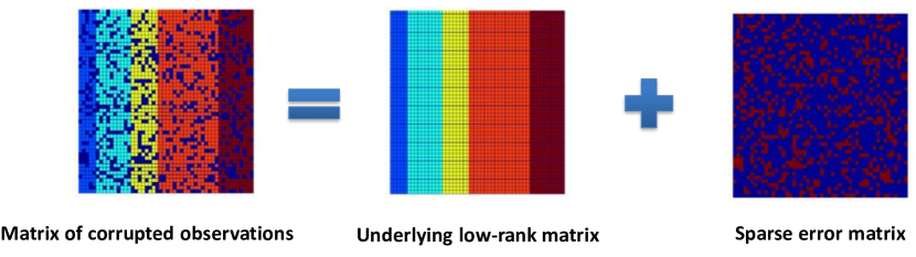
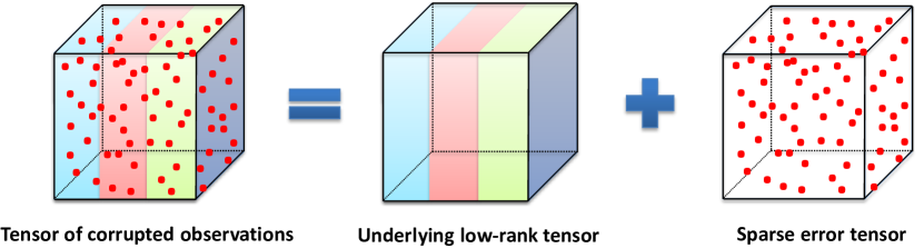
Figure 1: Illustrations of RPCA [RPCA] (up row) and our Tensor RPCA (bottom row). RPCA: low-rank and sparse matrix decomposition from noisy matrix observations. Tensor RPCA: low-rank and sparse tensor decomposition from noisy tensor observations.

The Robust PCA [RPCA] is the first polynomial-time algorithm with strong recovery guarantees. Suppose that we are given an observed matrix $\bm{X}\in\mathbb{R}^{n_{1}\times n_{2}}$, which can be decomposed as $\bm{X}=\bm{L}_{0}+\bm{E}_{0}$, where $\bm{L}_{0}$ is low-rank and $\bm{E}_{0}$ is sparse. It is shown in [RPCA] that if the singular vectors of $\bm{L}_{0}$ satisfy some incoherent conditions, e.g., $\bm{L}_{0}$ is low-rank and $\bm{E}_{0}$ is sufficiently sparse, then $\bm{L}_{0}$ and $\bm{E}_{0}$ can be exactly recovered with high probability by solving the following convex problem

$$\min_{\bm{L},\bm{E}}\ \lVert\bm{L}\rVert_{*}+\lambda\lVert\bm{E}\rVert_{1},\ {\text{s.t.}}\ \bm{X}=\bm{L}+\bm{E},$$ (1)

where $\lVert\bm{L}\rVert_{*}$ denotes the nuclear norm (sum of the singular values of $\bm{L}$), and $\lVert\bm{E}\rVert_{1}$ denotes the $\ell_{1}$-norm (sum of the absolute values of all the entries in $\bm{E}$). Theoretically, RPCA is guaranteed to work even if the rank of $\bm{L}_{0}$ grows almost linearly in the dimension of the matrix, and the errors in $\bm{E}_{0}$ are up to a constant fraction of all entries. The parameter $\lambda$ is suggested to be set as $1/\sqrt{\max(n_{1},n_{2})}$ which works well in practice. Algorithmically, program (1) can be solved by efficient algorithms, at a cost not too much higher than PCA. RPCA and its extensions have been successfully applied to background modeling [RPCA], subspace clustering [robustlrr], video compressive sensing [waters2011sparcs], etc.

One major shortcoming of RPCA is that it can only handle 2-way (matrix) data. However, real data is usually multi-dimensional in nature-the information is stored in multi-way arrays known as tensors [kolda2009tensor]. For example, a color image is a 3-way object with column, row and color modes; a greyscale video is indexed by two spatial variables and one temporal variable. To use RPCA, one has to first restructure the multi-way data into a matrix. Such a preprocessing usually leads to an information loss and would cause a performance degradation. To alleviate this issue, it is natural to consider extending RPCA to manipulate the tensor data by taking advantage of its multi-dimensional structure.

In this work, we are interested in the Tensor Robust Principal Component (TRPCA) model which aims to exactly recover a low-rank tensor corrupted by sparse errors. See Figure 1 for an intuitive illustration. More specifically, suppose that we are given a data tensor $\bm{\mathcal{X}}$, and know that it can be decomposed as

$$\bm{\mathcal{X}}=\bm{\mathcal{L}}_{0}+\bm{\mathcal{E}}_{0},$$ (2)

where $\bm{\mathcal{L}}_{0}$ is low-rank and $\bm{\mathcal{E}}_{0}$ is sparse, and both components are of arbitrary magnitudes. Note that we do not know the locations of the nonzero elements of $\bm{\mathcal{E}}_{0}$, not even how many there are. Now we consider a similar problem to RPCA. Can we recover the low-rank and sparse components exactly and efficiently from $\bm{\mathcal{X}}$? This is the problem of tensor RPCA studied in this work.

The tensor extension of RPCA is not easy since the numerical algebra of tensors is fraught with hardness results [hillar2013most], [anandkumar2016homotopy, zhang2018tensor]. A main issue is that the tensor rank is not well defined with a tight convex relaxation. Several tensor rank definitions and their convex relaxations have been proposed but each has its limitation. For example, the CP rank [kolda2009tensor], defined as the smallest number of rank one tensor decomposition, is generally NP-hard to compute. Also its convex relaxation is intractable. This makes the low CP rank tensor recovery challenging. The tractable Tucker rank [kolda2009tensor] and its convex relaxation are more widely used. For a $k$-way tensor $\bm{\mathcal{X}}$, the Tucker rank is a vector defined as $\text{rank}_{\text{tc}}(\bm{\mathcal{X}}):=\left(\text{rank}(\bm{X}^{\{1\}}),\text{rank}(\bm{X}^{\{2\}}),\cdots,\text{rank}(\bm{X}^{\{k\}})\right)$, where $\bm{X}^{\{i\}}$ is the mode-$i$ matricization of $\bm{\mathcal{X}}$ [kolda2009tensor]. Motivated by the fact that the nuclear norm is the convex envelope of the matrix rank within the unit ball of the spectral norm, the Sum of Nuclear Norms (SNN) [liu2013tensor], defined as $\sum_{i}\lVert\bm{X}^{\{i\}}\rVert_{*}$, is used as a convex surrogate of $\sum_{i}\text{rank}({\bm{X}^{\{i\}}})$. Then the work [mu2013square] considers the Low-Rank Tensor Completion (LRTC) model based on SNN:

$$\min_{\bm{\mathcal{X}}}\ \sum_{i=1}^{k}\lambda_{i}\lVert\bm{X}^{\{i\}}\rVert_{*},\ {\text{s.t.}}\ \bm{\mathcal{P}}_{\bm{{\Omega}}}(\bm{\mathcal{X}})=\bm{\mathcal{P}}_{\bm{{\Omega}}}(\bm{\mathcal{M}}),$$ (3)

where $\lambda_{i}>0$, and $\bm{\mathcal{P}}_{\bm{{\Omega}}}(\bm{\mathcal{X}})$ denotes the projection of $\bm{\mathcal{X}}$ on the observed set $\bm{{\Omega}}$. The effectiveness of this approach for image processing has been well studied in [liu2013tensor, tomioka2010estimation]. However, SNN is not the convex envelope of $\sum_{i}\text{rank}({\bm{X}^{\{i\}}})$ [romera2013new]. Actually, the above model can be substantially suboptimal [mu2013square]: reliably recovering a $k$-way tensor of length $n$ and Tucker rank $(r,r,\cdots,r)$ from Gaussian measurements requires $O(rn^{k-1})$ observations. In contrast, a certain (intractable) nonconvex formulation needs only $O(rK+nrK)$ observations. A better (but still suboptimal) convexification based on a more balanced matricization is proposed in [mu2013square]. The work [huang2014provable] presents the recovery guarantee for the SNN based tensor RPCA model

$$\min_{\bm{\mathcal{L}},\bm{\mathcal{E}}}\ \sum_{i=1}^{k}\lambda_{i}\lVert{\bm{L}}^{\{i\}}\rVert_{*}+\lVert\bm{\mathcal{E}}\rVert_{1},\ {\text{s.t.}}\ \bm{\mathcal{X}}=\bm{\mathcal{L}}+\bm{\mathcal{E}}.$$ (4)

A robust tensor CP decomposition problem is studied in [anandkumar2016tensor]. Though the recovery is guaranteed, the algorithm is nonconvex.

The limitations of existing works motivate us to consider an interesting problem: is it possible to define a new tensor nuclear norm such that it is a tight convex surrogate of certain tensor rank, and thus its resulting tensor RPCA enjoys a similar tight recovery guarantee to that of the matrix RPCA? This work will provide a positive answer to this question. Our solution is inspired by the recently proposed tensor-tensor product (t-product) [kilmer2011factorization] which is a generalization of the matrix-matrix product. It enjoys several similar properties to the matrix-matrix product. For example, based on t-product, any tensors have the tensor Singular Value Decomposition (t-SVD) and this motivates a new tensor rank, i.e., tensor tubal rank [kilmer2013third]. To recover a tensor of low tubal rank, we propose a new tensor nuclear norm which is rigorously induced by the t-product. First, the tensor spectral norm can be induced by the operator norm when treating the t-product as an operator. Then the tensor nuclear norm is defined as the dual norm of the tensor spectral norm. We further propose the tensor average rank (which is closely related to the tensor tubal rank), and prove that its convex envelope is the tensor nuclear norm within the unit ball of the tensor spectral norm. It is interesting that this framework, including the new tensor concepts and their relationships, is consistent with the one for the matrix cases. Equipped with these new tools, we then study the TRPCA problem which aims to recover the low tubal rank component $\bm{\mathcal{L}}_{0}$ and sparse component $\bm{\mathcal{E}}_{0}$ from noisy observations $\bm{\mathcal{X}}=\bm{\mathcal{L}}_{0}+\bm{\mathcal{E}}_{0}\in\mathbb{R}^{n_{1}\times n_{2}\times n_{3}}$ (this work focuses on the 3-way tensor) by convex optimization

$$\min_{\bm{\mathcal{L}},\ \bm{\mathcal{E}}}\ \lVert\bm{\mathcal{L}}\rVert_{*}+\lambda\lVert\bm{\mathcal{E}}\rVert_{1},\ {\text{s.t.}}\ \bm{\mathcal{X}}=\bm{\mathcal{L}}+\bm{\mathcal{E}},$$ (5)

where $\lVert\bm{\mathcal{L}}\rVert_{*}$ is our new tensor nuclear norm (see the definition in Section 3). We prove that under certain incoherence conditions, the solution to (5) perfectly recovers the low-rank and the sparse components, provided of course that the tubal rank of $\bm{\mathcal{L}}_{0}$ is not too large, and that $\bm{\mathcal{E}}_{0}$ is reasonably sparse. A remarkable fact, like in RPCA, is that (5) has no tunning parameter either. Our analysis shows that $\lambda=1/\sqrt{\max(n_{1},n_{2})n_{3}}$ guarantees the exact recovery when $\bm{\mathcal{L}}_{0}$ and $\bm{\mathcal{E}}_{0}$ satisfy certain assumptions. As a special case, if $\bm{\mathcal{X}}$ reduces to a matrix ($n_{3}=1$ in this case), all the new tensor concepts reduce to the matrix cases. Our TRPCA model (5) reduces to RPCA in (1), and also our recovery guarantee in Theorem LABEL:thm1 reduces to Theorem 1.1 in [RPCA]. Another advantage of (5) is that it can be solved by polynomial-time algorithms.

The contributions of this work are summarized as follows:

1. Motivated by the t-product [kilmer2011factorization] which is a natural generalization of the matrix-matrix product, we rigorously deduce a new tensor nuclear norm and some other related tensor concepts, and they own the same relationship as the matrix cases. This is the foundation for the extensions of the models, optimization method and theoretical analyzing techniques from matrix cases to tensor cases.

2. Equipped with the tensor nuclear norm, we theoretically show that under certain incoherence conditions, the solution to the convex TRPCA model (5) perfectly recovers the underlying low-rank component $\bm{\mathcal{L}}_{0}$ and sparse component $\bm{\mathcal{E}}_{0}$. RPCA [RPCA] and its recovery guarantee fall into our special cases.

3. We give a new rigorous proof of t-SVD factorization and a more efficient way than [lu2016tensorrpca] for solving TRPCA. We further perform several simulations to corroborate our theoretical results. Numerical experiments on images and videos also show the superiority of TRPCA over RPCA and SNN.

The rest of this paper is structured as follows. Section 2 gives some notations and preliminaries. Section 3 presents the way for defining the tensor nuclear norm induced by the t-product. Section LABEL:sec_tcTNN provides the recovery guarantee of TRPCA and the optimization details. Section LABEL:sec_exp presents numerical experiments conducted on synthetic and real data. We conclude this work in Section LABEL:sec_con.

2 Notations and Preliminaries

2.1 Notations

In this paper, we denote tensors by boldface Euler script letters, e.g., $\bm{\mathcal{A}}$. Matrices are denoted by boldface capital letters, e.g., $\bm{{A}}$; vectors are denoted by boldface lowercase letters, e.g., ${\bm{a}}$, and scalars are denoted by lowercase letters, e.g., $a$. We denote $\bm{I}_{n}$ as the $n\times n$ identity matrix. The fields of real numbers and complex numbers are denoted as $\mathbb{R}$ and $\mathbb{C}$, respectively. For a 3-way tensor $\bm{\mathcal{A}}\in\mathbb{C}^{n_{1}\times n_{2}\times n_{3}}$, we denote its $(i,j,k)$-th entry as $\bm{\mathcal{A}}_{ijk}$ or $a_{ijk}$ and use the Matlab notation $\bm{\mathcal{A}}(i,:,:)$, $\bm{\mathcal{A}}(:,i,:)$ and $\bm{\mathcal{A}}(:,:,i)$ to denote respectively the $i$-th horizontal, lateral and frontal slice (see definitions in [kolda2009tensor]). More often, the frontal slice $\bm{\mathcal{A}}(:,:,i)$ is denoted compactly as $\bm{{A}}^{(i)}$. The tube is denoted as $\bm{\mathcal{A}}(i,j,:)$. The inner product between $\bm{{A}}$ and $\bm{{B}}$ in $\mathbb{C}^{n_{1}\times n_{2}}$ is defined as ${\left\langle\bm{{A}},\bm{{B}}\right\rangle=\leavevmode\lstinline{{\lst@@@set@language\lst@@@set@numbers\lst@@@set@frame\lst@@@set@rulecolor\lst@@@set@language\footnotesize\small{\@listingGroup{ltx_lst_identifier}{Tr}}}}}(\bm{{A}}^{*}\bm{{B}})$, where $\bm{{A}}^{*}$ denotes the conjugate transpose of $\bm{{A}}$ and ${\leavevmode\lstinline{{\lst@@@set@language\lst@@@set@numbers\lst@@@set@frame\lst@@@set@rulecolor\lst@@@set@language\footnotesize\small{\@listingGroup{ltx_lst_identifier}{Tr}}}}}(\cdot)$ denotes the matrix trace. The inner product between $\bm{\mathcal{A}}$ and $\bm{\mathcal{B}}$ in $\mathbb{C}^{n_{1}\times n_{2}\times n_{3}}$ is defined as $\langle\bm{\mathcal{A}},\bm{\mathcal{B}}\rangle=\sum_{i=1}^{n_{3}}\left\langle\bm{{A}}^{(i)},\bm{{B}}^{(i)}\right\rangle$. For any $\bm{\mathcal{A}}\in\mathbb{C}^{n_{1}\times n_{2}\times n_{3}}$, the complex conjugate of $\bm{\mathcal{A}}$ is denoted as ${\leavevmode\lstinline{{\lst@@@set@language\lst@@@set@numbers\lst@@@set@frame\lst@@@set@rulecolor\lst@@@set@language\footnotesize\small{\@listingGroup{}{j}}}}}(\bm{\mathcal{A}})$ which takes the complex conjugate of each entry of $\bm{\mathcal{A}}$. We denote $\left\lfloor t\right\rfloor$ as the nearest integer less than or equal to $t$ and $\lceil t\rceil$ as the one greater than or equal to $t$.

Some norms of vector, matrix and tensor are used. We denote the $\ell_{1}$-norm as $\lVert\bm{\mathcal{A}}\rVert_{1}=\sum_{ijk}|a_{ijk}|$, the infinity norm as $\lVert\bm{\mathcal{A}}\rVert_{\infty}=\max_{ijk}|a_{ijk}|$ and the Frobenius norm as $\lVert\bm{\mathcal{A}}\rVert_{F}=\sqrt{\sum_{ijk}|a_{ijk}|^{2}}$, respectively. The above norms reduce to the vector or matrix norms if $\bm{\mathcal{A}}$ is a vector or a matrix. For ${\bm{v}}\in\mathbb{C}^{n}$, the $\ell_{2}$-norm is $\lVert{\bm{v}}\rVert_{2}=\sqrt{\sum_{i}|v_{i}|^{2}}$. The spectral norm of a matrix $\bm{{A}}$ is denoted as $\lVert\bm{{A}}\rVert=\max_{i}\sigma_{i}(\bm{{A}})$, where $\sigma_{i}(\bm{{A}})$’s are the singular values of $\bm{{A}}$. The matrix nuclear norm is $\lVert\bm{{A}}\rVert_{*}=\sum_{i}\sigma_{i}(\bm{{A}})$.

2.2 Discrete Fourier Transformation

The Discrete Fourier Transformation (DFT) plays a core role in tensor-tensor product introduced later. We give some related background knowledge and notations here. The DFT on ${\bm{v}}\in\mathbb{R}^{n}$, denoted as $\bar{\bm{v}}$, is given by

$$\bar{\bm{v}}=\bm{{F}}_{n}{\bm{v}}\in\mathbb{C}^{n},$$ (6)

where $\bm{{F}}_{n}$ is the DFT matrix defined as

$$\bm{{F}}_{n}=\begin{bmatrix}1&1&1&\cdots&1\\ 1&\omega&\omega^{2}&\cdots&\omega^{n-1}\\ \vdots&\vdots&\vdots&\ddots&\vdots\\ 1&\omega^{n-1}&\omega^{2(n-1)}&\cdots&\omega^{(n-1)(n-1)}\end{bmatrix}\in\mathbb{C}^{n\times n},$$

where $\omega={\text{e}}^{-\frac{2\pi i}{n}}$ is a primitive $n$-th root of unity in which $i=\sqrt{-1}$. Note that $\bm{{F}}_{n}/\sqrt{n}$ is a unitary matrix, i.e.,

$$\bm{{F}}_{n}^{*}\bm{{F}}_{n}=\bm{{F}}_{n}\bm{{F}}^{*}_{n}=n\bm{I}_{n}.$$ (7)

Thus $\bm{{F}}_{n}^{-1}=\bm{{F}}^{*}_{n}/n$. The above property will be frequently used in this paper. Computing $\bar{\bm{v}}$ by using (6) costs $O(n^{2})$. A more widely used method is the Fast Fourier Transform (FFT) which costs $O(n\log n)$. By using the Matlab command , we have ${\bar{\bm{v}}=\leavevmode\lstinline{{\lst@@@set@language\lst@@@set@numbers\lst@@@set@frame\lst@@@set@rulecolor\lst@@@set@language\footnotesize\small{\@listingGroup{}{}}}}}({\bm{v}})$. Denote the circulant matrix of ${\bm{v}}$ as

$${\displaystyle\leavevmode\lstinline{{\lst@@@set@language\lst@@@set@numbers\lst@@@set@frame\lst@@@set@rulecolor\lst@@@set@language\footnotesize\small{\@listingGroup{}{c}}}}}({\bm{v}})=\begin{bmatrix}v_{1}&v_{n}&\cdots&v_{2}\\ v_{2}&v_{1}&\cdots&v_{3}\\ \vdots&\vdots&\ddots&\vdots\\ v_{n}&v_{n-1}&\cdots&v_{1}\end{bmatrix}\in\mathbb{R}^{n\times n}.$$

It is known that it can be diagonalized by the DFT matrix, i.e.,

$${{\displaystyle\bm{{F}}_{n}\cdot\leavevmode\lstinline{{\lst@@@set@language\lst@@@set@numbers\lst@@@set@frame\lst@@@set@rulecolor\lst@@@set@language\footnotesize\small{\@listingGroup{}{c}}}}}({\bm{v}})\cdot\bm{{F}}_{n}^{-1}=\leavevmode\lstinline{{\lst@@@set@language\lst@@@set@numbers\lst@@@set@frame\lst@@@set@rulecolor\lst@@@set@language\footnotesize\small{\@listingGroup{}{g}}}}}(\bar{\bm{v}}),$$ (8)

where ${\leavevmode\lstinline{{\lst@@@set@language\lst@@@set@numbers\lst@@@set@frame\lst@@@set@rulecolor\lst@@@set@language\footnotesize\small{\@listingGroup{}{g}}}}}(\bar{\bm{v}})$ denotes a diagonal matrix with its $i$-th diagonal entry as $\bar{v}_{i}$. The above equation implies that the columns of $\bm{{F}}_{n}$ are the eigenvectors of ${(\leavevmode\lstinline{{\lst@@@set@language\lst@@@set@numbers\lst@@@set@frame\lst@@@set@rulecolor\lst@@@set@language\footnotesize\small{\@listingGroup{}{c}}}}}({\bm{v}}))^{\top}$ and $\bar{v}_{i}$’s are the corresponding eigenvalues.

Lemma 2.1.

[rojo2004some] Given any real vector ${\bm{v}}\in\mathbb{R}^{n}$, the associated $\bar{\bm{v}}$ satisfies

$${\displaystyle\bar{v}_{1}\in\mathbb{R}\text{ and }\leavevmode\lstinline{{\lst@@@set@language\lst@@@set@numbers\lst@@@set@frame\lst@@@set@rulecolor\lst@@@set@language\footnotesize\small{\@listingGroup{}{j}}}}}({\bar{v}}_{i})=\bar{v}_{n-i+2},\ i=2,\cdots,\left\lfloor\frac{n+1}{2}\right\rfloor.$$ (9)

Conversely, for any given complex $\bar{\bm{v}}\in\mathbb{C}^{n}$ satisfying (9), there exists a real block circulant matrix ${\leavevmode\lstinline{{\lst@@@set@language\lst@@@set@numbers\lst@@@set@frame\lst@@@set@rulecolor\lst@@@set@language\footnotesize\small{\@listingGroup{}{c}}}}}({\bm{v}})$ such that (8) holds.

As will be seen later, the above properties are useful for efficient computation and important for proofs. Now we consider the DFT on tensors. For $\bm{\mathcal{A}}\in\mathbb{R}^{n_{1}\times n_{2}\times n_{3}}$, we denote $\bm{\mathcal{\bar{A}}}\in\mathbb{C}^{n_{1}\times n_{2}\times n_{3}}$ as the result of DFT on $\bm{\mathcal{A}}$ along the 3-rd dimension, i.e., performing the DFT on all the tubes of $\bm{\mathcal{A}}$. By using the Matlab command , we have

$${\bm{\mathcal{\bar{A}}}=\leavevmode\lstinline{{\lst@@@set@language\lst@@@set@numbers\lst@@@set@frame\lst@@@set@rulecolor\lst@@@set@language\footnotesize\small{\@listingGroup{}{}}}}}(\bm{\mathcal{A}},[\ ],3).$$

In a similar fashion, we can compute $\bm{\mathcal{A}}$ from ${\bm{\mathcal{\bar{A}}}}$ using the inverse FFT, i.e.,

$${\bm{\mathcal{A}}=\leavevmode\lstinline{{\lst@@@set@language\lst@@@set@numbers\lst@@@set@frame\lst@@@set@rulecolor\lst@@@set@language\footnotesize\small{\@listingGroup{}{t}}}}}({\bm{\mathcal{\bar{A}}}},[\ ],3).$$

In particular, we denote $\bm{\bar{A}}\in\mathbb{C}^{n_{1}n_{3}\times n_{2}n_{3}}$ as a block diagonal matrix with its $i$-th block on the diagonal as the $i$-th frontal slice $\bm{\bar{A}}^{(i)}$ of ${\bm{\mathcal{\bar{A}}}}$, i.e.,

$${\bm{\bar{A}}=\leavevmode\lstinline{{\lst@@@set@language\lst@@@set@numbers\lst@@@set@frame\lst@@@set@rulecolor\lst@@@set@language\footnotesize\small{\@listingGroup{}{ag}}}}}(\bm{\mathcal{\bar{A}}})=\begin{bmatrix}\bm{\bar{A}}^{(1)}&&&\\ &\bm{\bar{A}}^{(2)}&&\\ &&\ddots&\\ &&&\bm{\bar{A}}^{(n_{3})}\end{bmatrix},$$

where ag is an operator which maps the tensor $\bm{\mathcal{\bar{A}}}$ to the block diagonal matrix $\bm{\bar{A}}$. Also, we define the block circulant matrix ${{\leavevmode\lstinline{{\lst@@@set@language\lst@@@set@numbers\lst@@@set@frame\lst@@@set@rulecolor\lst@@@set@language\footnotesize\small{\@listingGroup{}{rc}}}}}}(\bm{\mathcal{A}})\in\mathbb{R}^{n_{1}n_{3}\times n_{2}n_{3}}$ of $\bm{\mathcal{A}}$ as

$${\displaystyle{\leavevmode\lstinline{{\lst@@@set@language\lst@@@set@numbers\lst@@@set@frame\lst@@@set@rulecolor\lst@@@set@language\footnotesize\small{\@listingGroup{}{rc}}}}}}(\bm{\mathcal{A}})=\begin{bmatrix}\bm{{A}}^{(1)}&\bm{{A}}^{(n_{3})}&\cdots&\bm{{A}}^{(2)}\\ \bm{{A}}^{(2)}&\bm{{A}}^{(1)}&\cdots&\bm{{A}}^{(3)}\\ \vdots&\vdots&\ddots&\vdots\\ \bm{{A}}^{(n_{3})}&\bm{{A}}^{(n_{3}-1)}&\cdots&\bm{{A}}^{(1)}\end{bmatrix}.$$

Just like the circulant matrix which can be diagonalized by DFT, the block circulant matrix can be block diagonalized, i.e.,

$${\displaystyle(\bm{{F}}_{n_{3}}\otimes\bm{I}_{n_{1}})\cdot\leavevmode\lstinline{{\lst@@@set@language\lst@@@set@numbers\lst@@@set@frame\lst@@@set@rulecolor\lst@@@set@language\footnotesize\small{\@listingGroup{}{rc}}}}}(\bm{\mathcal{A}})\cdot(\bm{{F}}_{n_{3}}^{-1}\otimes\bm{I}_{n_{2}})=\bm{\bar{A}},$$ (10)

where $\otimes$ denotes the Kronecker product and $(\bm{{F}}_{n_{3}}\otimes\bm{I}_{n_{1}})/\sqrt{n_{3}}$ is unitary. By using Lemma 2.1, we have

$${\begin{cases}\bm{\bar{A}}^{(1)}\in\mathbb{R}^{n_{1}\times n_{2}},\\ \leavevmode\lstinline{{\lst@@@set@language\lst@@@set@numbers\lst@@@set@frame\lst@@@set@rulecolor\lst@@@set@language\footnotesize\small{\@listingGroup{}{j}}}}}({\bm{\bar{A}}}^{(i)})=\bm{\bar{A}}^{(n_{3}-i+2)},\ i=2,\cdots,\left\lfloor\frac{n_{3}+1}{2}\right\rfloor.\end{cases}$$ (11)

Conversely, for any given $\bm{\mathcal{\bar{A}}}\in\mathbb{C}^{n_{1}\times n_{2}\times n_{3}}$ satisfying (11), there exists a real tensor $\bm{\mathcal{A}}\in\mathbb{R}^{n_{1}\times n_{2}\times n_{3}}$ such that (10) holds. Also, by using (7), we have the following properties which will be used frequently:

$$\lVert\bm{\mathcal{A}}\rVert_{F}=\frac{1}{\sqrt{n_{3}}}\lVert\bm{\bar{A}}\rVert_{F},$$ (12)

$$\left\langle\bm{\mathcal{A}},\bm{\mathcal{B}}\right\rangle=\frac{1}{n_{3}}\left\langle\bm{\bar{A}},\bm{\bar{{B}}}\right\rangle.$$ (13)

2.3 T-product and T-SVD

For $\bm{\mathcal{A}}\in\mathbb{R}^{n_{1}\times n_{2}\times n_{3}}$, we define

$${{{\leavevmode\lstinline{{\lst@@@set@language\lst@@@set@numbers\lst@@@set@frame\lst@@@set@rulecolor\lst@@@set@language\footnotesize\small{\@listingGroup{}{old}}}}}(\bm{\mathcal{A}})=\begin{bmatrix}\bm{{A}}^{(1)}\\ \bm{{A}}^{(2)}\\ \vdots\\ \bm{{A}}^{(n_{3})}\end{bmatrix},\ \leavevmode\lstinline{{\lst@@@set@language\lst@@@set@numbers\lst@@@set@frame\lst@@@set@rulecolor\lst@@@set@language\footnotesize\small{\@listingGroup{}{d}}}}}(\leavevmode\lstinline{{\lst@@@set@language\lst@@@set@numbers\lst@@@set@frame\lst@@@set@rulecolor\lst@@@set@language\footnotesize\small{\@listingGroup{}{old}}}}}(\bm{\mathcal{A}}))=\bm{\mathcal{A}},$$

where the old operator maps $\bm{\mathcal{A}}$ to a matrix of size $n_{1}n_{3}\times n_{2}$ and d is its inverse operator.

Definition 2.1.

(T-product) [kilmer2011factorization] Let $\bm{\mathcal{A}}\in\mathbb{R}^{n_{1}\times n_{2}\times n_{3}}$ and $\bm{\mathcal{B}}\in\mathbb{R}^{n_{2}\times l\times n_{3}}$. Then the t-product $\bm{\mathcal{A}}*\bm{\mathcal{B}}$ is defined to be a tensor of size $n_{1}\times l\times n_{3}$,

$${{{\bm{\mathcal{A}}*\bm{\mathcal{B}}=\leavevmode\lstinline{{\lst@@@set@language\lst@@@set@numbers\lst@@@set@frame\lst@@@set@rulecolor\lst@@@set@language\footnotesize\small{\@listingGroup{}{d}}}}}(\leavevmode\lstinline{{\lst@@@set@language\lst@@@set@numbers\lst@@@set@frame\lst@@@set@rulecolor\lst@@@set@language\footnotesize\small{\@listingGroup{}{rc}}}}}(\bm{\mathcal{A}})\cdot\leavevmode\lstinline{{\lst@@@set@language\lst@@@set@numbers\lst@@@set@frame\lst@@@set@rulecolor\lst@@@set@language\footnotesize\small{\@listingGroup{}{old}}}}}(\bm{\mathcal{B}})).$$ (14)

The t-product can be understood from two perspectives. First, in the original domain, a 3-way tensor of size $n_{1}\times n_{2}\times n_{3}$ can be regarded as an $n_{1}\times n_{2}$ matrix with each entry being a tube that lies in the third dimension. Thus, the t-product is analogous to the matrix multiplication except that the circular convolution replaces the multiplication operation between the elements. Note that the t-product reduces to the standard matrix multiplication when $n_{3}=1$. This is a key observation which makes our tensor RPCA model shown later involve the matrix RPCA as a special case. Second, the t-product is equivalent to the matrix multiplication in the Fourier domain; that is, $\bm{\mathcal{C}}=\bm{\mathcal{A}}*\bm{\mathcal{B}}$ is equivalent to $\bm{\bar{C}}=\bm{\bar{A}}\bm{\bar{{B}}}$ due to (10). Indeed, $\bm{\mathcal{C}}=\bm{\mathcal{A}}*\bm{\mathcal{B}}$ implies

$${\displaystyle\leavevmode\lstinline{{\lst@@@set@language\lst@@@set@numbers\lst@@@set@frame\lst@@@set@rulecolor\lst@@@set@language\footnotesize\small{\@listingGroup{}{old}}}}}(\bm{\mathcal{C}})$$

$$= {{\displaystyle\leavevmode\lstinline{{\lst@@@set@language\lst@@@set@numbers\lst@@@set@frame\lst@@@set@rulecolor\lst@@@set@language\footnotesize\small{\@listingGroup{}{rc}}}}}(\bm{\mathcal{A}})\cdot\leavevmode\lstinline{{\lst@@@set@language\lst@@@set@numbers\lst@@@set@frame\lst@@@set@rulecolor\lst@@@set@language\footnotesize\small{\@listingGroup{}{old}}}}}(\bm{\mathcal{B}})$$

$$= {\displaystyle(\bm{{F}}_{n_{3}}^{-1}\otimes\bm{I}_{n_{1}})\cdot((\bm{{F}}_{n_{3}}\otimes\bm{I}_{n_{1}})\cdot\leavevmode\lstinline{{\lst@@@set@language\lst@@@set@numbers\lst@@@set@frame\lst@@@set@rulecolor\lst@@@set@language\footnotesize\small{\@listingGroup{}{rc}}}}}(\bm{\mathcal{A}})\cdot(\bm{{F}}_{n_{3}}^{-1}\otimes\bm{I}_{n_{2}}))$$

$${\displaystyle\cdot((\bm{{F}}_{n_{3}}\otimes\bm{I}_{n_{2}})\cdot\leavevmode\lstinline{{\lst@@@set@language\lst@@@set@numbers\lst@@@set@frame\lst@@@set@rulecolor\lst@@@set@language\footnotesize\small{\@listingGroup{}{old}}}}}(\bm{\mathcal{B}}))$$ (15)

$$= {\displaystyle(\bm{{F}}_{n_{3}}^{-1}\otimes\bm{I}_{n_{1}})\cdot\bm{\bar{A}}\cdot\leavevmode\lstinline{{\lst@@@set@language\lst@@@set@numbers\lst@@@set@frame\lst@@@set@rulecolor\lst@@@set@language\footnotesize\small{\@listingGroup{}{old}}}}}(\bm{\mathcal{\bar{B}}}),$$

where (15) uses (10). Left multiplying both sides with $(\bm{{F}}_{n_{3}}\otimes\bm{I}_{n_{1}})$ leads to ${{\leavevmode\lstinline{{\lst@@@set@language\lst@@@set@numbers\lst@@@set@frame\lst@@@set@rulecolor\lst@@@set@language\footnotesize\small{\@listingGroup{}{old}}}}}(\bm{\mathcal{\bar{C}}})=\bm{\bar{A}}\cdot\leavevmode\lstinline{{\lst@@@set@language\lst@@@set@numbers\lst@@@set@frame\lst@@@set@rulecolor\lst@@@set@language\footnotesize\small{\@listingGroup{}{old}}}}}(\bm{\mathcal{\bar{B}}})$. This is equivalent to $\bm{\bar{C}}=\bm{\bar{A}}\bm{\bar{{B}}}$. This property suggests an efficient way based on FFT to compute t-product instead of using (14). See Algorithm 1.

Algorithm 1 Tensor-Tensor Product

Input: $\bm{\mathcal{A}}\in\mathbb{R}^{n_{1}\times n_{2}\times n_{3}}$, $\bm{\mathcal{B}}\in\mathbb{R}^{n_{2}\times l\times n_{3}}$.
Output: $\bm{\mathcal{C}}=\bm{\mathcal{A}}*\bm{\mathcal{B}}\in\mathbb{R}^{n_{1}\times l\times n_{3}}$.

1. Compute ${\bm{\mathcal{\bar{A}}}=\leavevmode\lstinline{{\lst@@@set@language\lst@@@set@numbers\lst@@@set@frame\lst@@@set@rulecolor\lst@@@set@language\footnotesize\small{\@listingGroup{}{}}}}}(\bm{\mathcal{A}},[\ ],3)$ and ${\bm{\mathcal{\bar{B}}}=\leavevmode\lstinline{{\lst@@@set@language\lst@@@set@numbers\lst@@@set@frame\lst@@@set@rulecolor\lst@@@set@language\footnotesize\small{\@listingGroup{}{}}}}}(\bm{\mathcal{B}},[\ ],3)$.

2. Compute each frontal slice of $\bm{\mathcal{\bar{C}}}$ by

   $${\bm{\bar{C}}^{(i)}=\begin{cases}\bm{\bar{A}}^{(i)}\bm{\bar{{B}}}^{(i)},\quad&i=1,\cdots,\lceil\frac{n_{3}+1}{2}\rceil,\\ \leavevmode\lstinline{{\lst@@@set@language\lst@@@set@numbers\lst@@@set@frame\lst@@@set@rulecolor\lst@@@set@language\footnotesize\small{\@listingGroup{}{j}}}}}(\bm{\bar{C}}^{(n_{3}-i+2)}),\quad&i=\lceil\frac{n_{3}+1}{2}\rceil+1,\cdots,n_{3}.\end{cases}$$

3. Compute ${\bm{\mathcal{C}}=\leavevmode\lstinline{{\lst@@@set@language\lst@@@set@numbers\lst@@@set@frame\lst@@@set@rulecolor\lst@@@set@language\footnotesize\small{\@listingGroup{}{t}}}}}(\bm{\mathcal{\bar{C}}},[\ ],3)$.

The t-product enjoys many similar properties to the matrix-matrix product. For example, the t-product is associative, i.e., $\bm{\mathcal{A}}*(\bm{\mathcal{B}}*\bm{\mathcal{C}})=(\bm{\mathcal{A}}*\bm{\mathcal{B}})*\bm{\mathcal{C}}$. We also need some other concepts on tensors extended from the matrix cases.

Definition 2.2.

(Conjugate transpose) The conjugate transpose of a tensor $\bm{\mathcal{A}}\in\mathbb{C}^{n_{1}\times n_{2}\times n_{3}}$ is the tensor $\bm{\mathcal{A}}^{*}\in\mathbb{C}^{n_{2}\times n_{1}\times n_{3}}$ obtained by conjugate transposing each of the frontal slices and then reversing the order of transposed frontal slices 2 through $n_{3}$.

The tensor conjugate transpose extends the tensor transpose [kilmer2011factorization] for complex tensors. As an example, let $\bm{\mathcal{A}}\in\mathbb{C}^{n_{1}\times n_{2}\times 4}$ and its frontal slices be $\bm{{A}}_{1}$, $\bm{{A}}_{2}$, $\bm{{A}}_{3}$ and $\bm{{A}}_{4}$. Then

$${\displaystyle\bm{\mathcal{A}}^{*}=\leavevmode\lstinline{{\lst@@@set@language\lst@@@set@numbers\lst@@@set@frame\lst@@@set@rulecolor\lst@@@set@language\footnotesize\small{\@listingGroup{}{d}}}}}\left(\begin{bmatrix}\bm{{A}}_{1}^{*}\\ \bm{{A}}_{4}^{*}\\ \bm{{A}}_{3}^{*}\\ \bm{{A}}_{2}^{*}\end{bmatrix}\right).$$

Definition 2.3.

(Identity tensor) [kilmer2011factorization] The identity tensor $\bm{\mathcal{I}}\in\mathbb{R}^{n\times n\times n_{3}}$ is the tensor with its first frontal slice being the $n\times n$ identity matrix, and other frontal slices being all zeros.

It is clear that $\bm{\mathcal{A}}*\bm{\mathcal{I}}=\bm{\mathcal{A}}$ and $\bm{\mathcal{I}}*\bm{\mathcal{A}}=\bm{\mathcal{A}}$ given the appropriate dimensions. The tensor ${\bm{\mathcal{\bar{I}}}=\leavevmode\lstinline{{\lst@@@set@language\lst@@@set@numbers\lst@@@set@frame\lst@@@set@rulecolor\lst@@@set@language\footnotesize\small{\@listingGroup{}{}}}}}(\bm{\mathcal{I}},[\ ],3)$ is a tensor with each frontal slice being the identity matrix.

Definition 2.4.

(Orthogonal tensor) [kilmer2011factorization] A tensor $\bm{\mathcal{Q}}\in\mathbb{R}^{n\times n\times n_{3}}$ is orthogonal if it satisfies $\bm{\mathcal{Q}}^{*}*\bm{\mathcal{Q}}=\bm{\mathcal{Q}}*\bm{\mathcal{Q}}^{*}=\bm{\mathcal{I}}$.

Definition 2.5.

(F-diagonal Tensor) [kilmer2011factorization] A tensor is called f-diagonal if each of its frontal slices is a diagonal matrix.

Theorem 2.2.

(T-SVD) Let $\bm{\mathcal{A}}\in\mathbb{R}^{n_{1}\times n_{2}\times n_{3}}$. Then it can be factorized as

$$\bm{\mathcal{A}}=\bm{\mathcal{U}}*\bm{\mathcal{S}}*\bm{\mathcal{V}}^{*},$$ (16)

where $\bm{\mathcal{U}}\in\mathbb{R}^{n_{1}\times n_{1}\times n_{3}}$, $\bm{\mathcal{V}}\in\mathbb{R}^{n_{2}\times n_{2}\times n_{3}}$ are orthogonal, and $\bm{\mathcal{S}}\in\mathbb{R}^{n_{1}\times n_{2}\times n_{3}}$ is an f-diagonal tensor.

Proof.

The proof is by construction. Recall that (10) holds and $\bm{\bar{A}}^{(i)}$’s satisfy the property (11). Then we construct the SVD of each $\bm{\bar{A}}^{(i)}$ in the following way. For $i=1,\cdots,\lceil\frac{n_{3}+1}{2}\rceil$, let $\bm{\bar{A}}^{(i)}=\bm{\bar{U}}^{(i)}\bm{\bar{S}}^{(i)}(\bm{\bar{V}}^{(i)})^{*}$ be the full SVD of $\bm{\bar{A}}^{(i)}$. Here the singular values in $\bm{\bar{S}}^{(i)}$ are real. For $i=\lceil\frac{n_{3}+1}{2}\rceil+1,\cdots,n_{3}$, let ${\bm{\bar{U}}^{(i)}=\leavevmode\lstinline{{\lst@@@set@language\lst@@@set@numbers\lst@@@set@frame\lst@@@set@rulecolor\lst@@@set@language\footnotesize\small{\@listingGroup{}{j}}}}}(\bm{\bar{U}}^{(n_{3}-i+2)})$, $\bm{\bar{S}}^{(i)}=\bm{\bar{S}}^{(n_{3}-i+2)}$ and ${\bm{\bar{V}}^{(i)}=\leavevmode\lstinline{{\lst@@@set@language\lst@@@set@numbers\lst@@@set@frame\lst@@@set@rulecolor\lst@@@set@language\footnotesize\small{\@listingGroup{}{j}}}}}(\bm{\bar{V}}^{(n_{3}-i+2)})$. Then, it is easy to verify that $\bm{\bar{A}}^{(i)}=\bm{\bar{U}}^{(i)}\bm{\bar{S}}^{(i)}(\bm{\bar{V}}^{(i)})^{*}$ gives the full SVD of $\bm{\bar{A}}^{(i)}$ for $i=\lceil\frac{n_{3}+1}{2}\rceil+1,\cdots,n_{3}$. Then,

$$\bm{\bar{A}}=\bm{\bar{U}}\bm{\bar{S}}\bm{\bar{V}}^{*}.$$ (17)

By the construction of $\bm{\bar{U}}$, $\bm{\bar{S}}$ and $\bm{\bar{V}}$, and Lemma 2.1, we have that $(\bm{{F}}_{n_{3}}^{-1}\otimes\bm{I}_{n_{1}})\cdot\bm{\bar{U}}\cdot(\bm{{F}}_{n_{3}}\otimes\bm{I}_{n_{1}})$, $(\bm{{F}}_{n_{3}}^{-1}\otimes\bm{I}_{n_{1}})\cdot\bm{\bar{S}}\cdot(\bm{{F}}_{n_{3}}\otimes\bm{I}_{n_{2}})$ and $(\bm{{F}}_{n_{3}}^{-1}\otimes\bm{I}_{n_{2}})\cdot\bm{\bar{V}}\cdot(\bm{{F}}_{n_{3}}\otimes\bm{I}_{n_{2}})$ are real block circulant matrices. Then we can obtain an expression for ${\leavevmode\lstinline{{\lst@@@set@language\lst@@@set@numbers\lst@@@set@frame\lst@@@set@rulecolor\lst@@@set@language\footnotesize\small{\@listingGroup{}{rc}}}}}(\bm{\mathcal{A}})$ by applying the appropriate matrix $(\bm{{F}}_{n_{3}}^{-1}\otimes\bm{I}_{n_{1}})$ to the left and the appropriate matrix $(\bm{{F}}_{n_{3}}\otimes\bm{I}_{n_{2}})$ to the right of each of the matrices in (17), and folding up the result. This gives a decomposition of the form $\bm{\mathcal{U}}*\bm{\mathcal{S}}*\bm{\mathcal{V}}^{*}$, where $\bm{\mathcal{U}}$, $\bm{\mathcal{S}}$ and $\bm{\mathcal{V}}$ are real. ∎

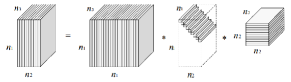
Figure 2: An illustration of the t-SVD of an $n_{1}\times n_{2}\times n_{3}$ tensor [hao2013facial].

Theorem 2.2 shows that any 3 way tensor can be factorized into 3 components, including 2 orthogonal tensors and an f-diagonal tensor. See Figure 2 for an intuitive illustration of the t-SVD factorization. T-SVD reduces to the matrix SVD when $n_{3}=1$. We would like to emphasize that the result of Theorem 2.2 was given first in [kilmer2011factorization] and later in some other related works [hao2013facial, martin2013order]. But their proof and the way for computing $\bm{\mathcal{U}}$ and $\bm{\mathcal{V}}$ are not rigorous. The issue is that their method cannot guarantee that $\bm{\mathcal{U}}$ and $\bm{\mathcal{V}}$ are real tensors. They construct each frontal slice $\bm{\bar{U}}^{(i)}$ (or $\bm{\bar{V}}^{(i)}$) of $\bm{\mathcal{\bar{U}}}$ (or $\bm{\mathcal{\bar{V}}}$ resp.) from the SVD of $\bm{\bar{A}}^{(i)}$ independently for all $i=1,\cdots,n_{3}$. However, the matrix SVD is not unique. Thus, $\bm{\bar{U}}^{(i)}$’s and $\bm{\bar{V}}^{(i)}$’s may not satisfy property (11) even though $\bm{\bar{A}}^{(i)}$’s do. In this case, the obtained $\bm{\mathcal{U}}$ (or $\bm{\mathcal{V}}$) from the inverse DFT of $\bm{\mathcal{\bar{U}}}$ (or $\bm{\mathcal{\bar{V}}}$ resp.) may not be real. Our proof above instead uses property (11) to construct $\bm{\mathcal{U}}$ and $\bm{\mathcal{V}}$ and thus avoids this issue. Our proof further leads to a more efficient way for computing t-SVD shown in Algorithm 2.

Algorithm 2 T-SVD

Input: $\bm{\mathcal{A}}\in\mathbb{R}^{n_{1}\times n_{2}\times n_{3}}$.
Output: T-SVD components $\bm{\mathcal{U}}$, $\bm{\mathcal{S}}$ and $\bm{\mathcal{V}}$ of $\bm{\mathcal{A}}$.

1. Compute ${\bm{\mathcal{\bar{A}}}=\leavevmode\lstinline{{\lst@@@set@language\lst@@@set@numbers\lst@@@set@frame\lst@@@set@rulecolor\lst@@@set@language\footnotesize\small{\@listingGroup{}{}}}}}(\bm{\mathcal{A}},[\ ],3)$.

2. Compute each frontal slice of $\bm{\mathcal{\bar{U}}}$, $\bm{\mathcal{\bar{S}}}$ and $\bm{\mathcal{\bar{V}}}$ from $\bm{\mathcal{\bar{A}}}$ by

   for $i=1,\cdots,\lceil\frac{n_{3}+1}{2}\rceil$ do

   $[\bm{\bar{U}}^{(i)},\bm{\bar{S}}^{(i)},\bm{\bar{V}}^{(i)}]=\text{SVD}(\bm{\bar{A}}^{(i)})$;

   end for

   for $i=\lceil\frac{n_{3}+1}{2}\rceil+1,\cdots,n_{3}$ do

   ${\bm{\bar{U}}^{(i)}=\leavevmode\lstinline{{\lst@@@set@language\lst@@@set@numbers\lst@@@set@frame\lst@@@set@rulecolor\lst@@@set@language\footnotesize\small{\@listingGroup{}{j}}}}}(\bm{\bar{U}}^{(n_{3}-i+2)})$;

   $\bm{\bar{S}}^{(i)}=\bm{\bar{S}}^{(n_{3}-i+2)}$;

   ${\bm{\bar{V}}^{(i)}=\leavevmode\lstinline{{\lst@@@set@language\lst@@@set@numbers\lst@@@set@frame\lst@@@set@rulecolor\lst@@@set@language\footnotesize\small{\@listingGroup{}{j}}}}}(\bm{\bar{V}}^{(n_{3}-i+2)})$;

   end for

3. Compute ${\bm{\mathcal{U}}=\leavevmode\lstinline{{\lst@@@set@language\lst@@@set@numbers\lst@@@set@frame\lst@@@set@rulecolor\lst@@@set@language\footnotesize\small{\@listingGroup{}{t}}}}}(\bm{\mathcal{\bar{U}}},[\ ],3)$, ${\bm{\mathcal{S}}=\leavevmode\lstinline{{\lst@@@set@language\lst@@@set@numbers\lst@@@set@frame\lst@@@set@rulecolor\lst@@@set@language\footnotesize\small{\@listingGroup{}{t}}}}}(\bm{\mathcal{\bar{S}}},[\ ],3)$, and ${\bm{\mathcal{V}}=\leavevmode\lstinline{{\lst@@@set@language\lst@@@set@numbers\lst@@@set@frame\lst@@@set@rulecolor\lst@@@set@language\footnotesize\small{\@listingGroup{}{t}}}}}(\bm{\mathcal{\bar{V}}},[\ ],3)$.

It is known that the singular values of a matrix have the decreasing order property. Let $\bm{\mathcal{A}}=\bm{\mathcal{U}}*\bm{\mathcal{S}}*\bm{\mathcal{V}}^{*}$ be the t-SVD of $\bm{\mathcal{A}}\in\mathbb{R}^{n_{1}\times n_{2}\times n_{3}}$. The entries on the diagonal of the first frontal slice $\bm{\mathcal{S}}(:,:,1)$ of $\bm{\mathcal{S}}$ have the same decreasing property, i.e.,

$$\bm{\mathcal{S}}(1,1,1)\geq\bm{\mathcal{S}}(2,2,1)\geq\cdots\geq\bm{\mathcal{S}}(n^{\prime},n^{\prime},1)\geq 0,$$ (18)

where $n^{\prime}=\min(n_{1},n_{2})$. The above property holds since the inverse DFT gives

$$\bm{\mathcal{S}}(i,i,1)=\frac{1}{n_{3}}\sum_{j=1}^{n_{3}}\bm{\mathcal{\bar{S}}}(i,i,j),$$ (19)

and the entries on the diagonal of $\bm{\mathcal{\bar{S}}}(:,:,j)$ are the singular values of $\bm{\mathcal{\bar{A}}}(:,:,j)$. As will be seen in Section 3, the tensor nuclear norm depends only on the first frontal slice $\bm{\mathcal{S}}(:,:,1)$. Thus, we call the entries on the diagonal of $\bm{\mathcal{S}}(:,:,1)$ as the singular values of $\bm{\mathcal{A}}$.

Definition 2.6.

(Tensor tubal rank) [kilmer2013third, zhang2014novel] For $\bm{\mathcal{A}}\in\mathbb{R}^{n_{1}\times n_{2}\times n_{3}}$, the tensor tubal rank, denoted as $\text{rank}_{\text{t}}(\bm{\mathcal{A}})$, is defined as the number of nonzero singular tubes of $\bm{\mathcal{S}}$, where $\bm{\mathcal{S}}$ is from the t-SVD of $\bm{\mathcal{A}}=\bm{\mathcal{U}}*\bm{\mathcal{S}}*\bm{\mathcal{V}}^{*}$. We can write

$$\text{rank}_{\text{t}}(\bm{\mathcal{A}})= \#\{i,\bm{\mathcal{S}}(i,i,:)\neq\bm{0}\}.$$

By using property (19), the tensor tubal rank is determined by the first frontal slice $\bm{\mathcal{S}}(:,:,1)$ of $\bm{\mathcal{S}}$, i.e.,

$$\text{rank}_{\text{t}}(\bm{\mathcal{A}})=\#\{i,\bm{\mathcal{S}}(i,i,1)\neq{0}\}.$$

Hence, the tensor tubal rank is equivalent to the number of nonzero singular values of $\bm{\mathcal{A}}$. This property is the same as the matrix case. Define $\bm{\mathcal{A}}_{k}=\sum_{i=1}^{k}\bm{\mathcal{U}}(:,i,:)*\bm{\mathcal{S}}(i,i,:)*\bm{\mathcal{V}}(:,i,:)^{*}$ for some $k<\min(n_{1},n_{2})$. Then $\bm{\mathcal{A}}_{k}=\arg\min_{\text{rank}_{\text{t}}(\tilde{\bm{\mathcal{A}}})\leq k}\lVert\bm{\mathcal{A}}-\tilde{\bm{\mathcal{A}}}\rVert_{F}$, so $\bm{\mathcal{A}}_{k}$ is the best approximation of $\bm{\mathcal{A}}$ with the tubal rank at most $k$. It is known that the real color images can be well approximated by low-rank matrices on the three channels independently. If we treat a color image as a three way tensor with each channel corresponding to a frontal slice, then it can be well approximated by a tensor of low tubal rank. A similar observation was found in [hao2013facial] with the application to facial recognition. Figure 3 gives an example to show that a color image can be well approximated by a low tubal rank tensor since most of the singular values of the corresponding tensor are relatively small.

In Section 3, we will define a new tensor nuclear norm which is the convex surrogate of the tensor average rank defined as follows. This rank is closely related to the tensor tubal rank.

Definition 2.7.

(Tensor average rank) For $\bm{\mathcal{A}}\in\mathbb{R}^{n_{1}\times n_{2}\times n_{3}}$, the tensor average rank, denoted as $\text{rank}_{\text{a}}(\bm{\mathcal{A}})$, is defined as

$${\displaystyle\text{rank}_{\text{a}}(\bm{\mathcal{A}})=\frac{1}{n_{3}}\text{rank}(\leavevmode\lstinline{{\lst@@@set@language\lst@@@set@numbers\lst@@@set@frame\lst@@@set@rulecolor\lst@@@set@language\footnotesize\small{\@listingGroup{}{rc}}}}}(\bm{\mathcal{A}})).$$ (20)

The above definition has a factor $\frac{1}{n_{3}}$. Note that this factor is crucial in this work as it guarantees that the convex envelope of the tensor average rank within a certain set is the tensor nuclear norm defined in Section 3. The underlying reason for this factor is the t-product definition. Each element of $\bm{\mathcal{A}}$ is repeated $n_{3}$ times in the block circulant matrix ${\leavevmode\lstinline{{\lst@@@set@language\lst@@@set@numbers\lst@@@set@frame\lst@@@set@rulecolor\lst@@@set@language\footnotesize\small{\@listingGroup{}{rc}}}}}(\bm{\mathcal{A}})$ used in the t-product. Intuitively, this factor alleviates such an entries expansion issue.

(a)

(b)

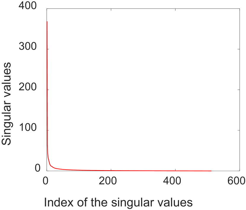
(c)

Figure 3: Color images can be approximated by low tubal rank tensors. (a) A color image can be modeled as a tensor $\bm{\mathcal{M}}\in\mathbb{R}^{512\times 512\times 3}$; (b) approximation by a tensor with tubal rank $r=50$; (c) plot of the singular values of $\bm{\mathcal{M}}$.

There are some connections between different tensor ranks and these properties imply that the low tubal rank or low average rank assumptions are reasonable for their applications in real visual data. First, $\text{rank}_{\text{a}}(\bm{\mathcal{A}})\leq\text{rank}_{\text{t}}(\bm{\mathcal{A}})$. Indeed,

$$\text{rank}_{\text{a}}(\bm{\mathcal{A}})=\frac{1}{n_{3}}\text{rank}(\bm{\bar{A}})\leq\max_{i=1,\cdots,n_{3}}\text{rank}(\bm{\bar{A}}^{(i)})=\text{rank}_{\text{t}}(\bm{\mathcal{A}}),$$

where the first equality uses (10). This implies that a low tubal rank tensor always has low average rank. Second, let $\text{rank}_{\text{tc}}(\bm{\mathcal{A}})=\left(\text{rank}(\bm{{A}}^{\{1\}}),\text{rank}(\bm{{A}}^{\{2\}}),\text{rank}(\bm{{A}}^{\{3\}})\right)$, where $\bm{{A}}^{\{i\}}$ is the mode-$i$ matricization of $\bm{\mathcal{A}}$, be the Tucker rank of $\bm{\mathcal{A}}$. Then $\text{rank}_{\text{a}}(\bm{\mathcal{A}})\leq\text{rank}(\bm{{A}}^{\{1\}})$. This implies that a tensor with low Tucker rank has low average rank. The low Tucker rank assumption used in some applications, e.g., image completion [liu2013tensor], is applicable to the low average rank assumption. Third, if the CP rank of $\bm{\mathcal{A}}$ is $r$, then its tubal rank is at most $r$ [zhang2015exact]. Let $\bm{\mathcal{A}}=\sum_{i=1}^{r}{\bm{a}}_{i}^{(1)}\circ{\bm{a}}_{i}^{(2)}\circ{\bm{a}}_{i}^{(3)}$, where $\circ$ denotes the outer product, be the CP decomposition of $\bm{\mathcal{A}}$. Then $\bm{\mathcal{\bar{A}}}=\sum_{i=1}^{r}{\bm{a}}_{i}^{(1)}\circ{\bm{a}}_{i}^{(2)}\circ\bar{{\bm{a}}}_{i}^{(3)}$, where ${\bar{{\bm{a}}}_{i}^{(3)}=\leavevmode\lstinline{{\lst@@@set@language\lst@@@set@numbers\lst@@@set@frame\lst@@@set@rulecolor\lst@@@set@language\footnotesize\small{\@listingGroup{}{}}}}}({\bm{a}}_{i}^{(3)})$. So $\bm{\mathcal{\bar{A}}}$ has the CP rank at most $r$, and each frontal slice of $\bm{\mathcal{\bar{A}}}$ is the sum of $r$ rank-1 matrices. Thus, the tubal rank of $\bm{\mathcal{A}}$ is at most $r$. In summary, we show that the low average rank assumption is weaker than the low Tucker rank and low CP rank assumptions.

3 Tensor Nuclear Norm (TNN)

In this section, we propose a new tensor nuclear norm which is a convex surrogate of tensor average rank. Based on t-SVD, one may have many different ways to define the tensor nuclear norm intuitively. We give a new and rigorous way to deduce the tensor nuclear norm from the t-product, such that the concepts and their properties are consistent with the matrix cases. This is important since it guarantees that the theoretical analysis of the tensor nuclear norm based tensor RPCA model in Section LABEL:sec_tcTNN can be done in a similar way to RPCA. Figure 4 summarizes the way for the new definitions and their relationships. It begins with the known operator norm [atkinson2009theoretical] and t-product. First, the tensor spectral norm is induced by the tensor operator norm by treating the t-product as an operator. Then the tensor nuclear norm is defined as the dual norm of the tensor spectral norm. Finally, we show that the tensor nuclear norm is the convex envelope of the tensor average rank within the unit ball of the tensor spectral norm.

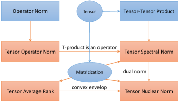
Figure 4: An illustration of the way to define the tensor nuclear norm and the relationship with other tensor concepts. First, the tensor operator norm is a special case of the known operator norm performed on the tensors. The tensor spectral norm is induced by the tensor operator norm by treating the tensor-tensor product as an operator. Then the tensor nuclear norm is defined as the dual norm of the tensor spectral norm. We also define the tensor average rank and show that its convex envelope is the tensor nuclear norm within the unit ball of the tensor spectral norm. As detailed in Section 3, the tensor spectral norm, tensor nuclear norm and tensor average rank are also defined on the matricization of the tensor.

Let us first recall the concept of operator norm [atkinson2009theoretical]. Let $(V,\lVert\cdot\rVert_{V})$ and $(W,\lVert\cdot\rVert_{W})$ be normed linear spaces and $L:V\rightarrow W$ be the bounded linear operator between them, respectively. The operator norm of $L$ is defined as

$$\lVert L\rVert=\sup_{\lVert{\bm{v}}\rVert_{V}\leq 1}\lVert L({\bm{v}})\rVert_{W}.$$ (21)

Let $V=\mathbb{C}^{n_{2}}$, $W=\mathbb{C}^{n_{1}}$ and $L({\bm{v}})=\bm{{A}}{\bm{v}}$, ${\bm{v}}\in V$, where $\bm{{A}}\in\mathbb{C}^{n_{1}\times n_{2}}$. Based on different choices of $\lVert\cdot\rVert_{V}$ and $\lVert\cdot\rVert_{W}$, many matrix norms can be induced by the operator norm in (21). For example, if $\lVert\cdot\rVert_{V}$ and $\lVert\cdot\rVert_{W}$ are $\lVert\cdot\rVert_{F}$, then the operator norm (21) reduces to the matrix spectral norm.

Now, consider the normed linear spaces $(V,\lVert\cdot\rVert_{F})$ and $(W,\lVert\cdot\rVert_{F})$, where $V=\mathbb{R}^{n_{2}\times 1\times n_{3}}$, $W=\mathbb{R}^{n_{1}\times 1\times n_{3}}$, and $\bm{\mathcal{L}}:V\rightarrow W$ is a bounded linear operator. In this case, (21) reduces to the tensor operator norm

$$\lVert\bm{\mathcal{L}}\rVert=\sup_{\lVert\bm{\mathcal{V}}\rVert_{F}\leq 1}\lVert\bm{\mathcal{L}}(\bm{\mathcal{V}})\rVert_{F}.$$ (22)

As a special case, if $\bm{\mathcal{L}}(\bm{\mathcal{V}})=\bm{\mathcal{A}}*\bm{\mathcal{V}}$, where $\bm{\mathcal{A}}\in\mathbb{R}^{n_{1}\times n_{2}\times n_{3}}$ and $\bm{\mathcal{V}}\in V$, then the tensor operator norm (22) gives the tensor spectral norm, denoted as $\lVert\bm{\mathcal{A}}\rVert$,

$$\lVert\bm{\mathcal{A}}\rVert:= \sup_{\lVert\bm{\mathcal{V}}\rVert_{F}\leq 1}\lVert\bm{\mathcal{A}}*\bm{\mathcal{V}}\rVert_{F}$$

$$= {{\displaystyle\sup_{\lVert\bm{\mathcal{V}}\rVert_{F}\leq 1}\lVert\leavevmode\lstinline{{\lst@@@set@language\lst@@@set@numbers\lst@@@set@frame\lst@@@set@rulecolor\lst@@@set@language\footnotesize\small{\@listingGroup{}{rc}}}}}(\bm{\mathcal{A}})\cdot\leavevmode\lstinline{{\lst@@@set@language\lst@@@set@numbers\lst@@@set@frame\lst@@@set@rulecolor\lst@@@set@language\footnotesize\small{\@listingGroup{}{old}}}}}(\bm{\mathcal{V}})\rVert_{F}$$ (23)

$$= {\displaystyle\lVert\leavevmode\lstinline{{\lst@@@set@language\lst@@@set@numbers\lst@@@set@frame\lst@@@set@rulecolor\lst@@@set@language\footnotesize\small{\@listingGroup{}{rc}}}}}(\bm{\mathcal{A}})\rVert,$$ (24)

where (23) uses (14), and (24) uses the definition of matrix spectral norm.

Definition 3.1.

(Tensor spectral norm) The tensor spectral norm of $\bm{\mathcal{A}}\in\mathbb{R}^{n_{1}\times n_{2}\times n_{3}}$ is defined as ${\lVert\bm{\mathcal{A}}\rVert:=\lVert\leavevmode\lstinline{{\lst@@@set@language\lst@@@set@numbers\lst@@@set@frame\lst@@@set@rulecolor\lst@@@set@language\footnotesize\small{\@listingGroup{}{rc}}}}}(\bm{\mathcal{A}})\rVert$.

TABLE I: Parallelism of sparse vector, low-rank matrix and low-rank tensor.

	Sparse vector	Low-rank matrix	Low-rank tensor (this work)
Degeneracy of	1-D signal $\bm{x}\in\mathbb{R}^{n}$	2-D correlated signals $\bm{X}\in\mathbb{R}^{n_{1}\times n_{2}}$	3-D correlated signals $\bm{\mathcal{X}}\in\mathbb{R}^{n_{1}\times n_{2}\times n_{3}}$
Parsimony concept	cardinality	rank	tensor average rank
Measure	$\ell_{0}$-norm $\lVert\bm{x}\rVert_{0}$	$\text{rank}(\bm{X})$	$\text{rank}_{\text{a}}(\bm{\mathcal{X}})$
Convex surrogate	$\ell_{1}$-norm $\lVert\bm{x}\rVert_{1}$	nuclear norm $\lVert\bm{X}\rVert_{*}$	tensor nuclear norm $\lVert\bm{\mathcal{X}}\rVert_{*}$
Dual norm	$\ell_{\infty}$-norm $\lVert\bm{x}\rVert_{\infty}$	spectral norm $\lVert\bm{X}\rVert$	tensor spectral norm $\lVert\bm{\mathcal{X}}\rVert$

Strictly speaking, the tensor tubal rank, which bounds the tensor average rank, is also the parsimony concept of the low-rank tensor.

By (7) and (10), we have

$${\displaystyle\lVert\bm{\mathcal{A}}\rVert=\lVert\leavevmode\lstinline{{\lst@@@set@language\lst@@@set@numbers\lst@@@set@frame\lst@@@set@rulecolor\lst@@@set@language\footnotesize\small{\@listingGroup{}{rc}}}}}(\bm{\mathcal{A}})\rVert=\lVert\bm{\bar{A}}\rVert.$$ (25)

This property is frequently used in this work. It is known that the matrix nuclear norm is the dual norm of the matrix spectral norm. Thus, we define the tensor nuclear norm, denoted as $\lVert\bm{\mathcal{A}}\rVert_{*}$, as the dual norm of the tensor spectral norm. For any $\bm{\mathcal{B}}\in\mathbb{R}^{n_{1}\times n_{2}\times n_{3}}$ and $\bm{\tilde{{B}}}\in\mathbb{C}^{n_{1}n_{3}\times n_{2}n_{3}}$, we have

$$\lVert\bm{\mathcal{A}}\rVert_{*}:= \sup_{\lVert\bm{\mathcal{B}}\rVert\leq 1}\langle{\bm{\mathcal{A}}},{\bm{\mathcal{B}}}\rangle$$ (26)

$$= \sup_{\lVert\bm{\bar{{B}}}\rVert\leq 1}\frac{1}{n_{3}}\langle{\bm{\bar{A}}},{\bm{\bar{{B}}}}\rangle$$ (27)

$$\leq \frac{1}{n_{3}}\sup_{\lVert\bm{\tilde{{B}}}\rVert\leq 1}|\langle{\bm{\bar{A}}},{\bm{\tilde{{B}}}}\rangle|$$ (28)

$$= \frac{1}{n_{3}}\lVert\bm{\bar{A}}\rVert_{*},$$ (29)

$$= {\displaystyle\frac{1}{n_{3}}\lVert\leavevmode\lstinline{{\lst@@@set@language\lst@@@set@numbers\lst@@@set@frame\lst@@@set@rulecolor\lst@@@set@language\footnotesize\small{\@listingGroup{}{rc}}}}}(\bm{\mathcal{A}})\rVert_{*},$$ (30)

where (27) is from (13), (28) is due to the fact that $\bm{\bar{{B}}}$ is a block diagonal matrix in $\mathbb{C}^{n_{1}n_{3}\times n_{2}n_{3}}$ while $\bm{\tilde{{B}}}$ is an arbitrary matrix in $\mathbb{C}^{n_{1}n_{3}\times n_{2}n_{3}}$, (29) uses the fact that the matrix nuclear norm is the dual norm of the matrix spectral norm, and (30) uses (10) and (7). Now we show that there exists $\bm{\mathcal{B}}\in\mathbb{R}^{n_{1}\times n_{2}\times n_{3}}$ such that the equality (28) holds and thus ${\lVert\bm{\mathcal{A}}\rVert_{*}=\frac{1}{n_{3}}\lVert\leavevmode\lstinline{{\lst@@@set@language\lst@@@set@numbers\lst@@@set@frame\lst@@@set@rulecolor\lst@@@set@language\footnotesize\small{\@listingGroup{}{rc}}}}}(\bm{\mathcal{A}})\rVert_{*}$. Let $\bm{\mathcal{A}}=\bm{\mathcal{U}}*\bm{\mathcal{S}}*\bm{\mathcal{V}}^{*}$ be the t-SVD of $\bm{\mathcal{A}}$ and $\bm{\mathcal{B}}=\bm{\mathcal{U}}*\bm{\mathcal{V}}^{*}$. We have

$$\langle{\bm{\mathcal{A}}},{\bm{\mathcal{B}}}\rangle= \langle{\bm{\mathcal{U}}*\bm{\mathcal{S}}*\bm{\mathcal{V}}^{*}},{\bm{\mathcal{U}}*\bm{\mathcal{V}}^{*}}\rangle$$ (31)

$$= \frac{1}{n_{3}}\left\langle\overline{\bm{\mathcal{U}}*\bm{\mathcal{S}}*\bm{\mathcal{V}}^{*}},\overline{\bm{\mathcal{U}}*\bm{\mathcal{V}}^{*}}\right\rangle$$

$$= {\displaystyle\frac{1}{n_{3}}\left\langle\bm{\bar{U}}\bm{\bar{S}}\bm{\bar{V}}^{*},\bm{\bar{U}}\bm{\bar{V}}^{*}\right\rangle=\frac{1}{n_{3}}\leavevmode\lstinline{{\lst@@@set@language\lst@@@set@numbers\lst@@@set@frame\lst@@@set@rulecolor\lst@@@set@language\footnotesize\small{\@listingGroup{ltx_lst_identifier}{Tr}}}}}(\bm{\bar{S}})$$

$$= {\displaystyle\frac{1}{n_{3}}\lVert\bm{\bar{A}}\rVert_{*}=\frac{1}{n_{3}}\lVert\leavevmode\lstinline{{\lst@@@set@language\lst@@@set@numbers\lst@@@set@frame\lst@@@set@rulecolor\lst@@@set@language\footnotesize\small{\@listingGroup{}{rc}}}}}(\bm{\mathcal{A}})\rVert_{*}.$$ (32)

Combining (26)-(30) and (31)-(32) leads to ${\lVert\bm{\mathcal{A}}\rVert_{*}=\frac{1}{n_{3}}\lVert\leavevmode\lstinline{{\lst@@@set@language\lst@@@set@numbers\lst@@@set@frame\lst@@@set@rulecolor\lst@@@set@language\footnotesize\small{\@listingGroup{}{rc}}}}}(\bm{\mathcal{A}})\rVert_{*}$. On the other hand, by (31)-(32), we have

$$\lVert\bm{\mathcal{A}}\rVert_{*}= \langle{\bm{\mathcal{U}}*\bm{\mathcal{S}}*\bm{\mathcal{V}}^{*}},{\bm{\mathcal{U}}*\bm{\mathcal{V}}^{*}}\rangle$$

$$= \langle{\bm{\mathcal{U}}^{*}*\bm{\mathcal{U}}*\bm{\mathcal{S}}},{\bm{\mathcal{V}}^{*}*\bm{\mathcal{V}}}\rangle$$

$$= \langle{\bm{\mathcal{S}}},\bm{\mathcal{I}}\rangle=\sum_{i=1}^{r}\bm{\mathcal{S}}(i,i,1),$$ (33)

where $r=\text{rank}_{\text{t}}(\bm{\mathcal{A}})$ is the tubal rank. Thus, we have the following definition of tensor nuclear norm.

Definition 3.2.

(Tensor nuclear norm) Let $\bm{\mathcal{A}}=\bm{\mathcal{U}}*\bm{\mathcal{S}}*\bm{\mathcal{V}}^{*}$ be the t-SVD of $\bm{\mathcal{A}}\in\mathbb{R}^{n_{1}\times n_{2}\times n_{3}}$. The tensor nuclear norm of $\bm{\mathcal{A}}$ is defined as

$$\lVert\bm{\mathcal{A}}\rVert_{*}:=\left\langle\bm{\mathcal{S}},\bm{\mathcal{I}}\right\rangle=\sum_{i=1}^{r}\bm{\mathcal{S}}(i,i,1),$$

where $r=\text{rank}_{\text{t}}(\bm{\mathcal{A}})$.

From (33), it can be seen that only the information in the first frontal slice of $\bm{\mathcal{S}}$ is used when defining the tensor nuclear norm. Note that this is the first work which directly uses the singular values $\bm{\mathcal{S}}(:,:,1)$ of a tensor to define the tensor nuclear norm. Such a definition makes it consistent with the matrix nuclear norm. The above TNN definition is also different from existing works [lu2016tensorrpca, zhang2014novel, semerci2014tensor].

It is known that the matrix nuclear norm $\lVert\bm{{A}}\rVert_{*}$ is the convex envelope of the matrix rank $\text{rank}(\bm{{A}})$ within the set $\{\bm{{A}}|\lVert\bm{{A}}\rVert\leq 1\}$ [fazel2002matrix]. Now we show that the tensor average rank and tensor nuclear norm have the same relationship.

Theorem 3.1.

On the set $\{\bm{\mathcal{A}}\in\mathbb{R}^{n_{1}\times n_{2}\times n_{3}}|\lVert\bm{\mathcal{A}}\rVert\leq 1\}$, the convex envelope of the tensor average rank $\text{rank}_{\text{a}}(\bm{\mathcal{A}})$ is the tensor nuclear norm $\lVert\bm{\mathcal{A}}\rVert_{*}$.

We would like to emphasize that the proposed tensor spectral norm, tensor nuclear norm and tensor ranks are not arbitrarily defined. They are rigorously induced by the t-product and t-SVD. These concepts and their relationships are consistent with the matrix cases. This is important for the proofs, analysis and computation in optimization. Table I summarizes the parallel concepts in sparse vector, low-rank matrix and low-rank tensor. With these elements in place, the existing proofs of low-rank matrix recovery provide a template for the more general case of low-rank tensor recovery.

Also, from the above discussions, we have the property

(34)