Search for Food of Birds, Fish and Insects

3.1 Introduction

When you are out in a forest searching for mushrooms you wish to fill your basket with these delicacies as quickly as possible. But how do you search efficiently for them if you have no clue where they grow (Fig. 3.1)? The answer to this question is not only relevant for finding mushrooms CBV15 ; Kla15 . It also helps to understand how white blood cells kill efficiently intruding pathogens HaBa12 , how monkeys search for food in a tropical forest RFM03 , and how to optimize the hunt for submarines Shles06 .

Figure 3.1: Illustration of a typical search problem CBV15 ; Kla15 : A human searcher endeavours to find mushrooms that are randomly distributed in a certain area. It would help to have an optimal search strategy that enables one to find as many mushrooms as possible by minimizing the search time.

In society the problem to develop efficient search strategies belongs to the realm of operations research, the mathematical optimization of organizational problems in order to aid human decision-making Stone07 . Examples are the search for landmines, castaways or victims of avalanches. Over the past two decades search research Shles06 attracted particular attention within the fields of ecology and biology. The new discipline of movement ecology Nath08 ; MCB14 studies foraging strategies of biological organisms: Prominent examples are wandering albatrosses searching for food Vis96 ; Vis99 ; Edw07 , marine predators diving for prey Sims08 ; Sims10 , and bees collecting nectar LICCK12 ; LCK13 . Within this context the Lévy Flight Hypothesis (LFH) became especially popular: It predicts that under certain mathematical conditions on the type of food sources long Lévy flights SZK93 minimize the search time Vis96 ; Vis99 ; VLRS11 . This implies that for a bumblebee searching for rare flowers the flight lengths should be distributed according to a power law. Remarkably, the prediction by the LFH is completely different from the paradigm put forward by Karl Pearson more than a century ago Pea06 , who proposed to model the movements of biological organisms by simple random walks as introduced in Chap. 2 of this book. His suggestion entails that the movement lengths are distributed exponentially according to a Gaussian distribution, see Eq.(2.10) in this section. Lévy and Gaussian processes represent fundamental but different classes of diffusive spreading. Both are justified by a rigorous mathematical underpinning.

More than 60 years ago Gnedenko and Kolmogorov proved mathematically that specific types of power laws, called Lévy stable distributions KRS08 ; ZDK15 , obey a central limit theorem. Their result generalizes the conventional central limit theorem for Gaussian distributions, which explains why Brownian motion is observed in a huge variety of physical phenomena. But exponential tails decay faster than power laws, which implies that for Lévy-distributed flight lengths there is a larger probability to yield long flights than for flight lengths obeying Gaussian statistics. Consequently, Lévy flights should be better suited to detect sparsely, randomly distributed targets than Brownian motion, which in turn should outperform Lévy motion when the targets are dense. This is the basic idea underlying the LFH. Empirical tests of it, however, are hotly debated Edw07 ; Buch08 ; dJWH11 ; Pyke15 ; Reyn15 : Not only are there problems with a sound statistical analysis of experimental data sets when checking for power laws; their biological interpretation is also often unclear: For example, for monkeys living in a tropical forest who feed on specific types of fruit it is not clear whether the observed Lévy flights of the monkeys are due to the distribution of the trees on which their preferred fruit grows, or whether the monkeys’ Lévy motion represents an evolutionary adapted optimal search strategy helping them to survive RFM03 . Theoretically the LFH was motivated by random walk models with Lévy-distributed step lengths that were solved in computer simulations Vis99 . A rigorous mathematical proof of the LFH remains elusive.

This chapter introduces to the following fundamental question cross-linking the fields of ecology, biology, physics and mathematics: Can search for food by biological organisms be understood by mathematical modeling? BLMV11 ; VLRS11 ; MCB14 ; ZDK15 It consists of three main parts: Section 3.2 reviews the LFH. Section 3.3 outlines the controversial discussion about its verification by including basics about the theory of Lévy motion. Section 3.4 illustrates the need to go beyond the LFH by elaborating on bumblebee flights. We summarize our discussion in Sec. 3.5.

3.2 Lévy motion and the Lévy Flight Hypothesis

3.2.1 Lévy flights of wandering albatrosses

In 1996 Gandhimohan Viswanathan and collaborators published a pioneering article in the journal Nature Vis96 . For albatrosses foraging in the South Atlantic the flight times were recorded by putting sensors at their feet. The sensors got wet when the birds were diving for food, see the inset of Fig. 3.2. The duration of a flight was thus defined by the period of time when a sensor remained dry, terminated by a dive for catching food. The main part of Fig. 3.2 shows a histogram of the flight time intervals of some albatrosses. The straight line represents a Lévy stable distribution proportional to $\sim t^{-\mu}$ with an exponent of $\mu=2$. By assuming that the albatrosses move with an on average constant speed one can associate these flight times with a respective power law distribution of flight lengths. This suggests that the albatrosses were searching for food by performing Lévy flights.

For more than a decade albatrosses were considered to be the most prominent example of an animal performing Lévy flights. This work triggered a large number of related studies suggesting that many other animals like deer, bumblebees, spider monkeys and fishes also perform Lévy motion Vis99 ; RFM03 ; Sims08 ; Sims10 ; VLRS11 .

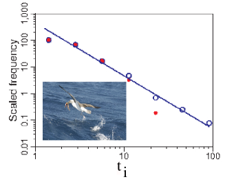
Figure 3.2: Histogram where ‘scaled frequencies’ holds for the number of flight time intervals of length $t_{i}$ (in hours) normalized by their respective bin widths. The data is for five albatrosses during 19 foraging bouts (double-logarithmic scale). Blue open circles show the data from Ref. Vis96 . The straight line indicates a power law $\sim t^{-\mu}$ with exponent $\mu=2$. The red filled circles are adjusted flight durations using the same data set by eliminating times that the birds spent on an island Edw07 . The histogram is reprinted by permission from Macmillan Publishers Ltd: Nature Ref. Edw07 , copyright 2007. The inset shows an albatross catching food; reprinted by permission from Macmillan Publishers Ltd: Nature Ref. Shles06 , copyright 2006.

3.2.2 The Lévy Flight Hypothesis

In 1999 the group around Gandhimohan Viswanathan published another important article in Nature Vis99 . Here the approach was more theoretical by posing, and addressing, the following general question:

“What is the best statistical strategy to adapt in order to search efficiently for randomly located objects?”

To answer this question they introduced a special type of what is called a Lévy walk ZDK15 in two dimensions and studied it both by computer simulations and by analytical approximations. Their model consists of point targets randomly distributed in a plane and a (point) forager moving with constant speed. If the forager spots a target within a pre-defined finite vision distance, it moves to the target directly. Otherwise the forager chooses a direction at random with a jump length $\ell$ randomly drawn from a Lévy stable distribution $\sim\ell^{-\mu}\>,\>1\leq\mu\leq 3$. While the forager is moving it constantly looks out for targets within the given vision distance. If no target is detected, the forager stops after the given distance and repeats the process.

Although these rules look simple enough, there are some subtleties that exemplify the problem of mathematically modeling a biological foraging problem:

1. Here we have chosen what is called a cruise forager, i.e., a forager that senses targets whenever it is moving. In contrast, a saltaltory forager would not sense a target while moving. It needs to land close to a target within a given radius of perception in order to find it JPP09 .

2. For a cruise forager a jump is terminated when it hits a target, hence this model defines a truncated Lévy walk Sims10 .

3. One has to decide whether a forager eliminates targets when it finds them or not, i.e., whether it performs destructive or non-destructive search Vis99 . As we will see below, whether a monkey eats a fruit thus effectively eliminating it, at least for a long time, or whether a bee collects nectar from a flower that replenishes quickly defines mathematically different foraging problems.

4. We have not yet said anything about the density of the targets.

5. We have deliberately assumed that the targets are immobile, which may not always be realistic for a biological foraging problem (e.g., marine predators Sims08 ; Sims10 ).

6. If we ask about the best strategy to search efficiently, how do we define optimality?

These few points illustrate the difficulty to relate abtract mathematical random walk models to biological foraging reality. Interestingly, the motion generated by these models often sensitively depends on right such details: In Ref. Vis99 foraging efficiency was defined as the ratio of the number of targets found divided by the total distance traveled by a forager, see Eq.(3) therein. Different definitions are possible, depend on the type of forager and may yield different results JPP09 . The foraging efficiency was then computed in Ref. Vis99 under variation of the exponent $\mu$ of the above Lévy distribution generating the jump length. The results led to what was coined the Lévy Flight Hypothesis (LFH), which we formulate as follows:

Lévy motion provides an optimal search strategy for sparse, randomly distributed, immobile, revisitable targets in unbounded domains.

Intuitively this result can be understood as follows: Fig. 3.3 (left) displays a typical trajectory of a Brownian walker. One can see that this dynamics is ‘more localized’ while Lévy motion shown in Fig. 3.3 (right) depicts clusters interrupted by long jumps. It thus makes sense that Brownian motion is better suited to find targets that are densely distributed while Lévy motion outperforms Brownian motion when targets are sparse, since it avoids oversampling due to long jumps. The reason why the targets need to be revisitable is that the exponent $\mu$ of the Lévy distribution depends on whether the search is destructive or not, cf. the third point on the list of foraging conditions above: For non-destructive foraging $\mu=2$ was found to be optimal while for destructive foraging $\mu=1$ maximized the foraging efficiency, which corresponds to the special case of ballistic flights ZDK15 . The reason for these different exponents is that destructive foraging changes the distribution and the density of the targets thus selecting a different foraging strategy to be optimal.

     

Figure 3.3: Brownian motion (left) vs. Lévy motion (right) in the plane, illustrated by typical trajectories.

3.3 Lévy or not Lévy?

3.3.1 Revisiting Lévy flights of wandering albatrosses

Several years passed before the results by Viswanathan et al. were revisited in another Nature article led by Andrew Edwards Edw07 : When analyzing new, larger and more precise data for foraging albatrosses the old results of Ref. Vis96 could not be recovered, see Fig. 1 in Ref. Edw07 . This led the researchers to reconsider the old albatross data. A correction of these data sets yielded the result shown in Fig. 3.2 as the red filled circles: One can see that the Lévy stable law with an exponent of $\mu=2$ for the flight times is gone. Instead the data now seems to be fit best with a gamma distribution.

What happened is explained in Ref. Buch08 : For all measurements the sensors were put onto the feet of the albatrosses when the birds were sitting on an island, and at this point the measurement process was started. However, to this time the sensors were dry; and in Ref. Vis96 these times were interpreted as Lévy flights. The same applied to the end of a foraging bout when the birds were back on the island. Subtracting these erroneous time intervals from the data sets eliminated the Lévy flights.

However, in Ref. HWQ12 yet new albatross data was analyzed, and the old data from Refs. Vis96 ; Edw07 was again reanalyzed: This time truncated power laws were used for the analysis, and furthermore data sets for individual birds were tested instead of pooling together the data for all birds. In this reference it was concluded that some individual albatross indeed do perform Lévy flights while others do not.

3.3.2 The Lévy Flight Paradigm

The debate about the LFH created a surge of publications testing it both theoretically and experimentally; see Refs. BLMV11 ; VLRS11 ; MCB14 ; ZDK15 for reviews. But experimentally it is difficult to verify the mathematical conditions on which the LFH formulated in Sec. 3.2.2 is based. Often the LFH was thus interpreted in a much looser sense by ignoring any mathematical assumptions in terms of what one may call the Lévy Flight Paradigm (LFP):

Look for power laws in the probability distributions of step lengths of foraging animals.

We illustrate virtues and pitfalls related to the LFP by data from Ref. Sims10 on the diving depths of free-ranging marine predators. Impressively, in this work over 12 million movement displacements were recorded and analyzed for 14 different species. As an example, Fig. 3.4 shows results for a blue shark: Plotted at the bottom are probability distributions of its diving depths, called move step length frequency distribution, where a step length is defined as the distance moved by the shark per unit time. Included are fits to a truncated power law and to an exponential distribution. Since here Lévy distributions were used whose longest step lengths were cut off, the fits do not consist of straight lines but are bent off, in contrast to Fig. 3.2. The top of this figure depicts the corresponding time series from which the data was extracted, split into five different sections. Each section is characterized by profoundly different average diving depths. These different sections correspond to the shark being in different regions of the ocean, i.e., either on-shelf or off-shelf. It was argued that on-shelf, where the diving depth of the shark is very limited, the data can be better fitted with an exponential distribution (sections f and h) while off-shelf the data displays power-law behavior with an exponent close to two (sections g, i and j). Fig. 3.4 thus suggests a strong dependence of the foraging dynamics on the environment in which it takes place, where the latter defines the food distribution. Related switching behavior between power law-like Lévy and exponential Brownian motion search strategies was reported for microzooplankton, jellyfish and mussels.

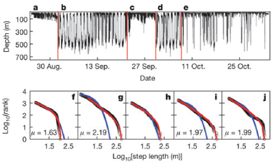
Figure 3.4: Top: time series of the diving depth of a blue shark. The red lines split the data into different sections (a - e), where the shark dives deep or the diving depth is more constrained. These sections match to the shark being off-shelf or on the shelf, respectively. Bottom: double-logarithmic plots of the move step length frequency distribution (‘rank’) as a function of the step length, which is the vertical distance moved by the shark per unit time, with the notation (f - j) corresponding to the primary data shown in sections (a - e). Black circles correspond to data, red lines to fits with truncated power laws of exponent $\mu$, blue lines to exponential fits. This figure is reprinted by permission from Macmillan Publishers Ltd: Nature Ref. Sims10 , copyright 2010.

The power law matching to the data in the off-shelf regions was interpreted in support of the LFH. However, note the periodic oscillations displayed by the time series at the top of Fig. 3.4. Upon closer inspection they reveal a 24h day-night cycle: During the night the shark hovers close to the surface of the sea while over the day it dives for food. For the move step length distributions shown in Fig. 3.4 the data was averaged over all these periodic oscillations. But the distributions in sections g, i and j all show a ‘wiggle’ on a finer scale. This suggests to better fit the data by a superposition of two different distributions LICCK12 taking into account that day and night define two very different phases of motion, instead of using only one function by averaging over all times. Apart from this, one may argue that this analysis does not test for the original LFH put forward in Ref. Vis96 . But this requires a bit more knowledge about the theory of Lévy motion; we will come back to this point in Sec. 3.3.5.

3.3.3 Two different Lévy Flight Hypotheses

Our discussion in the previous sections suggests to distinguish between two different LFHs:

1. The first is the ‘conventional’ one that we formulated in Sec. 3.2.2, originally put forward in Ref. Vis96 : It may now be further specified as the Lévy Search Hypothesis (LSH), because it suggests that under certain conditions Lévy flights represent an optimal search strategy. Here optimality needs to be defined rigorously mathematically. This can be done in different ways given the specific biological situation at hand that one wishes to model JPP09 . Typically optimality within this context aims at minimizing the search time for finding targets. The interesting biological interpretation of the LSH is that it has been evolved in biological organisms as an evolutionary adaptive strategy that maximizes the success for survival. The LSH version of the LFH became most popular.

2. In parallel there is a second type of LFH, which may be called the Lévy Environmental Hypothesis (LEH): It suggests that Lévy flights emerge from the interaction between a forager and a food source distribution. The latter may be scale-free thus directly inducing the Lévy flights. This is in sharp contrast to the LSH, which suggests that under certain conditions a forager performs Lévy flights irrespective of the actual food source distribution. Emergence of novel patterns and dynamics due to the interaction of the single parts of a complex system with each other, on the other hand, is at the heart of the theory of complex systems. The LEH is the hypothesis that to some extent was formulated in Ref. Vis96 , but it became more popular rather later on RFM03 ; Sims08 ; Sims10 .

Both the LSH and the LEH are bound together by what we called the Lévy Flight Paradigm (LFP) in Sec. 3.3.2. The LFP extracts the formal essence from both these different hypotheses by proposing to look for power laws in the probability distributions of foraging dynamics by ignoring any conditions of validity of these two hypotheses. Consequently, in contrast to the LSH and LEH the mathematical, physical and biological origin and meaning of power laws obtained by following the LFP is typically not clear. On the other hand, the LFP motivated to take a fresh look at foraging data sets by not only testing for exponential distributions. It widened the scope by emphasizing that one should also check for power laws in animal movement data.

3.3.4 Intermittent search strategies as an alternative to Lévy motion

Simple random walks as introduced in Section 2.1 represent examples of unimodal types of motion if the random step lengths are sampled from only one specific distribution. For example, choosing a Gaussian distribution we obtain Brownian motion while a Lévy-stable distribution produces Lévy flights. Combining two different types of motion like Brownian and Lévy yields bimodal motion. A simple example is shown in Fig. 3.5: Imagine you have lost your keys at home, but you have a vague idea where to find them. Hence, you are running straightforwardly to the location where you expect them to be. This may be modeled as a ballistic flight during which you quickly relocate, say, from the kitchen to the study room. However, when you arrive in your study room you should switch to a different type of motion, which is suitably adapted to locally search the environment. For this mode you may choose, e.g., Brownian motion. The resulting dynamics is called intermittent BLMV11 : It consists of two different phases of motion mixed randomly, which in our example are ballistic relocation events and local Brownian motion.

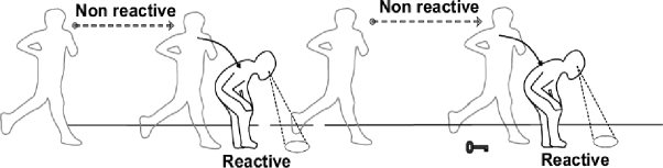
Figure 3.5: Illustration of an intermittent search strategy: A human searcher looks for a target (key) by alternating between two different modes of motion. During fast, ballistic relocation phases the searcher is not able to detect any target (non reactive). These phases are interrupted by slow phases of Brownian motion during which a searcher is able to detect a target (reactive) BLMV11 .

This type of motion can be exploited to search efficiently in the following way: You may not bother to look for your keys while you are walking from the kitchen to the study room. You are more interested to get from point A to point B as quickly as possible, and while doing so your search mode is switched off. This is called a non reactive phase in Fig. 3.5. But as you expect the keys to be in your study room, while switching to Brownian motion therein you simultaneously switch on your scanning abilities. This defines your local search mode called reactive in Fig. 3.5. Correspondingly, for aninmals one may imagine that during a fast relocation event, or flight, they are unable to detect any targets while their sensory mechanisms become active during slow local search. This is close to what was called a saltaltory forager in Sec. 3.2.2, but this forager did not feature any local search dynamics.

Intermittent search dynamics can be modeled by writing down a set of two coupled equations, one that generates ballistic flights and another one that yields Brownian motion. The coupling captures the switching between both modes. One furthermore needs to model that search is only performed during the Brownian motion mode. By analyzing a respective ballistic-Brownian system of equations it was found that this dynamics yields a minimum of a suitably defined search time under parameter variation if a target is non-revisitable, i.e., it is destroyed once it is found. Note that for targets that are non-replenishing the Lévy walks of Ref. Vis99 did not yield any non-trivial optimization of the search time. Instead, they converged to pure ballistic flights as being optimal. The LSH, in turn, only applies to revisitable, i.e., replenishing targets. Hence intermittent motion poses no contradiction. A popular account of this result was given by Michael Shlesinger in his Nature article ‘How to hunt a submarine?’ Shles06 .

3.3.5 Theory of Lévy flights in a nutshell

We now briefly elaborate on the theory of Lévy motion. This section may be skipped by a reader who is not so interested in theoretical foundations. We recommend Ref. SZK93 for an outline of this topic from a physics point of view and Chap. 5 in Ref. KRS08 for a more mathematical introduction. We start from the simple random walk on the line introduced in Chap. 2 of this book,

$$x_{n+1}=x_{n}+\ell_{n}\quad,$$ (3.1)

where $x_{n}$ is the position of a random walker at discrete time $n\in\mathbb{N}$ moving in one dimension, and $\ell_{n}=x_{n+1}-x_{n}$ defines the jump of length $|\ell_{n}|$ between two positions. In Chap. 2 the special case of constant jump length $|\ell_{n}|=\ell$ was considered, where the sign of the jump was randomly determined by tossing a coin with, say, plus for heads and minus for tails. The coin was furthermore supposed to be fair in the sense of yielding equal probabilities for heads and tails. This simple random walk can be generalized by considering a bigger variety of jumps. Mathematically this is modeled by drawing the random variable $\ell_{n}$ from some more general probability distribution than featuring only probability one half for each of two outcomes. For example, instead we could draw $\ell_{n}$ at each time step $n$ randomly from a uniform distribution, where each jump between $-L$ and $L$ is equally possible given by the probability density $\rho(\ell_{n})=1/(2L)\>,\>-L\leq\ell_{n}\leq L$ and zero otherwise. Alternatively, we could allow arbitrarily large jumps by drawing $\ell_{n}$ from an unbounded Gaussian distribution, see Eq.(2.10) in Chap. 2 (by replacing $x$ therein with $\ell_{n}$ and setting $t$ constant). For both generalized random walks Eq. (3.1) would still reproduce in the long time limit the fundamental diffusive properties Eq. (4) discussed in Chap. 2, i.e., the linear growth in time of the mean square displacement, and Eq. (2.10) in Chap. 2, the Gaussian probability distribution for the position $x_{n}$ of a walker at time step $n$. This follows mathematically from the conventional central limit theorem.

We now further generalize the random walk Eq. (3.1) in a more non-trivial way by randomly drawing $\ell_{n}$ from a Lévy $\alpha$-stable distribution KRS08 ,

$$\rho(\ell_{n})\sim|\ell_{n}|^{-1-\alpha}\>(|\ell_{n}|\gg 1)\>,\>0<\alpha<2\>,$$ (3.2)

characterized by power law tails in the limit of large $|\ell_{n}|$. This functional form is in sharp contrast to the exponential tails of Gaussian distributions and has important consequences, as it violates one of the assumptions on which the conventional central limit theorem rests. However, for the range of exponents $\alpha$ stated above it can be shown that these distributions obey a generalized central limit theorem: The proof employs the fact that these distributions are stable, in the sense that a linear combination of two random variables sampled independently from the same distribution reproduces the very same distribution, up to some scale factors SZK93 . This in turn implies that Lévy stable distributions are scale invariant and thus self-similar. Physically one speaks of $\ell_{n}$ sampled independently and identically distributed from Eq. (3.2) as white Lévy noise. As by definition there are no correlations between the random variables $\ell_{n}$ the stochastic process generated by Eq. (3.1) is memoryless, meaning at time step $(n+1)$ the particle has no memory where it came from at any previous time step $n$. In mathematics this is called a Markov processes, and Lévy flights belong to this important class of stochastic processes.

What we presented here is only a very rough, mathematically rather imprecise outline of how to define an $\alpha$-stable Lévy process generating Lévy flights. Especially, the function in Eq. (3.2) is not defined for small $\ell_{n}$, as the given power law diverges for $\ell_{n}\to 0$. A rigorous definition of Lévy stable distributions is obtained by using the characteristic function of this process, i.e., the Fourier transform of its probability distribution, which is well-defined analytically. The full probability distribution can then be generated from it SZK93 ; KRS08 . For $\alpha=2$ this approach reproduces Gaussian distributions, hence Lévy dynamics suitably generalizes Brownian motion SZK93 ; KRS08 .

Another important property of Lévy stable distributions is that the mean squared flight length of a Lévy walker does not exist,

$$\langle\ell_{n}^{2}\rangle=\int_{-\infty}^{\infty}\;d\ell_{n}\;\rho(\ell_{n})\ell_{n}^{2}=\infty\>.$$ (3.3)

The above equation defines what is called the second moment of the probability distribution $\rho(\ell_{n})$. Higher moments are defined analogously by $\langle\ell^{k}\rangle\>,\>k\in\mathbb{N}$, and for Lévy distributions they are also infinite. This means that in contrast to simple random walks generating Brownian motion, see again Chap. 2, Lévy motion does not have any characteristic length scale. However, since moments are rather easily obtained from experimental data this poses a problem to Lévy flights as a viable physical model to be validated by experiments.

This problem can be solved by using the very related concept of Lévy walks ZDK15 : These are random walks where again jumps are drawn randomly from the Lévy stable distribution Eq. (3.2). But as a penalty for long jumps the walker spends a time $t_{n}$ proportional to the length of the jump to complete it, $t_{n}=v\ell_{n}$, where the proportionality factor $v$, typically chosen as $|v|=const.$, defines the velocity of the Lévy walker. This implies that both jump lengths $\ell_{n}$ and flight times $t_{n}$ are distributed according to the same power law. In contrast, for the Lévy flights introduced above a walker makes a jump of length $|\ell_{n}|$ during an integer time step of duration $\Delta n=1$, which implies that contrary to a Lévy walker a Lévy flyer can jump instantaneously over arbitrarily long distances with arbitrarily large velocities.

Lévy walks belong to the broad and important class of continuous time random walks MeKl00 ; KRS08 ; KlSo11 , which further generalize ordinary random walks by allowing a walker to move by non-integer time steps. We do not discuss all the similarities and differences between Lévy walks and Lévy flights, see Ref. ZDK15 for details, but instead highlight only one important fact: While for Lévy flights the mean square displacement $\langle x^{2}\rangle$, see Eq.(1) in Chap. 2, does not exist, which follows from our discussion above, for Lévy walks it does. This is due to the finite velocities, which truncate the power law tails in the probability distributions for the positions of a Lévy walker. However, in contrast to Brownian motion where it grows linearly in time as shown in Chap. 2, see Eq.(2), for Lévy walks it grows faster than linear,

$$\langle x^{2}\rangle\sim t^{\gamma}\>(t\to\infty)\>,$$ (3.4)

with $\gamma>1$. If $\gamma\neq 1$ one speaks of anomalous diffusion MeKl00 ; KRS08 . The case $\gamma>1$ is called superdiffusion, since a particle diffuses faster than Brownian motion, correspondingly $\gamma<1$ refers to subdiffusion. There is a wealth of different stochastic models exhibiting anomalous diffusion, and while superdiffusion appears to be more common among foraging biological organisms than subdiffusion the whole spectrum of anomalous diffusion is found in a variety of different processes in the natural sciences, and even in the human world MeKl00 ; MeKl04 ; KRS08 .

Often the difference between Lévy walks and flights is not quite appreciated in the experimental literature, see, e.g., Fig. 3.4, where move step length frequency distributions were plotted. By definition a move step length $x$ per unit time corresponds to what we defined as a jump length $\ell_{n}$ by Eq. (3.1) above, $x=\ell_{n}$. Hence, a truncated power law fit $\sim x^{-\mu}$ to the distributions plotted in Fig. 3.4 corresponds to a fit with a truncated form of the jump length distribution Eq. (3.2) with exponent $\mu=1+\alpha$ testing for truncated Lévy flights ZDK15 . The truncation cures the problem of infinite moments exhibited by random walks based on ordinary Lévy flights mentioned above. However, this analysis does not test the LFH put forward in Ref Vis99 , which was derived from Lévy walks. But checking for Lévy walks requires an entirely different data analysis HaBa12 ; ZDK15 .

3.4 Beyond the Lévy Flight Hypothesis: foraging bumblebees

The LFH and its variants illustrated the problem to which extent biologically relevant search strategies may be identified by mathematical modeling. What we then formulated as the LFP in Sec. 3.3.2 motivated to generally look for power laws in the probability distributions of step lengths of foraging animals. Inspired by the long debate about the different functional forms of move step lengths probability distributions, and by further diluting the LFP, an even weaker guiding principle would be to assume that the foraging dynamics of biological organisms can be understood by analyzing such probability distributions alone. In the following we discuss an experiment, and its theoretical analysis, which illustrate that one may miss crucial information by studying only probability distributions. In that respect, this last section provides a look beyond the LFH that focuses on such distributions.

3.4.1 Bumblebees foraging under predation risk

In Refs. Ings08 Thomas Ings and Lars Chittka reported a laboratory experiment in which environmental foraging conditions were varied in a fully controlled manner. The question they addressed with this experiment was whether changes of environmental conditions, in this case exposing bumblebees to predation threat or not, led to changes in their foraging dynamics. This question was answered by a statistical analysis of the bumblebee flights recorded in this experiment on both spatial and temporal scales LICCK12 .

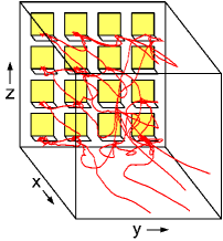
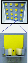
(a)     (b)     (c)

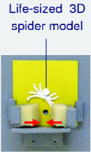
Figure 3.6: Illustration of a laboratory experiment investigating the dynamics of bumblebees foraging under predation risk: (a) Sketch of the cubic foraging arena together with part of the flight trajectory of a single bumblebee. The bumblebees forage on a grid of artificial flowers on one side of the box. While being on the landing platforms, they have access to nectar. All flowers can be equipped with spider models and trapping mechanisms simulating predation attempts as shown in (b), (c) Ings08 ; LICCK12 .

The experiment is sketched in Fig. 3.6: Bumblebees (Bombus terrestris) were flying in a cubic arena of $\approx$ 75cm side length by foraging on a 4$\times$4 vertical grid of artificial yellow flowers on one wall. The 3D flight trajectories of 30 bumblebees, tested sequentially and individually, were tracked by two high frame rate cameras. On the landing platform of each flower nectar was given to the bumblebees and replenished after consumption. To analyze differences in the foraging behavior of the bumblebees under threat of predation, artificial spiders were introduced. The experiment was staged into several different phases of which, however, only the following three are relevant to our analysis:

1. spider-free foraging

2. foraging under predation risk

3. a memory test one day later

Before and directly after stage 2 the bumblebees were trained to forage in the presence of artificial spiders, which were randomly placed on 25% of the flowers. A spider was emulated by a spider model on the flower and a trapping mechanism, which briefly held the bumblebee to simulate a predation attempt. In stages 2 and 3 the spider models were present but the traps were inactive in order to analyze the influence of previous experience with predation risk on the bumblebees’ flight dynamics; see Ref Ings08 for full details of the experimental setup and staging.

It is important to observe that neither the LSH nor the LEH can be tested by this experiment, as the flight arena is too small: The bumblebees always sense the walls and may adjust their flight behavior accordingly. However, there is a cross-link to the LEH in that this experiment studies the interaction of a forager with the environment, and its consequences for the dynamics of the forager, in a very controlled way. The weaker guiding principle derived from the LFP that we discussed above furthermore suggests that the main information to understand the foraging dynamics may be contained in the probability distributions of flight step lengths only. On this basis one may naively expect to see different step lengths probability distributions emerging by changing the environmental conditions, which here is the predation risk.

3.4.2 Velocity distributions vs. velocity correlations: experimental results

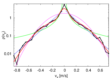
Figure 3.7: Semi-logarithmic plot of the distribution of velocities $v_{y}$ parallel to the $y$-axis in Fig. 3.6(a) (black crosses) for a single bumblebee in the spider-free stage 1. The different lines represent maximum likelihood fits with a Gaussian mixture (red line), exponential (blue dotted), power law (green dashed), and single Gaussian distribution (violet dotted) LICCK12 .

Figure 3.7 shows a typical probability distribution of the horizontal velocities parallel to the flower wall (cf. the y-direction in Fig. 3.6(a)) for a single bumblebee. This distribution is in analogy to the move step length frequency distributions of the shark shown in Fig. 3.4, which also represent velocity distributions if the depicted step lengths are divided by the corresponding constant time intervals of their measurements as discussed in Sec. 3.3.5. The distribution of bumblebee flights per unit time is characterized by a peak at low velocities. Only a power law and a Gaussian distribution can immediately be ruled out by visual inspection as matching functional forms. However, a mixture of two Gaussian distributions and an exponential function appear to be equally possible. Maximum likelihood fits supplemented by respective information criteria yielded the former as the most likely functional form matching the data. This result can be understood biologically as representing two different flight modes near a flower versus far away from it, which is confirmed by spatially separated data analysis LICCK12 . That the bumblebee switches to a specific distribution of lower velocities when approaching a flower reflects a spatially adapted flight mode to accessing the food sources. As a result, here we encounter another version of intermittent motion: In contrast to the temporal switching between different flight modes discussed in Sec. 3.3.4 this one is due to switching in different regions of space.

Surprisingly, when extracting the velocity distributions of single bumblebees at the three different stages of the experiment and comparing their best fits with each other, qualitatively and quantitatively no differences could be found in these distributions between the spider-free stage and the stages where artificial spider models were present LICCK12 . This means that the bumblebees fly with the very same statistical distribution of velocities irrespective of whether predators are present or not. The answer about possible changes in the bumblebee flights due to changes in the environmental conditions is thus not given by analyzing the probability distributions of move step lengths, as one may infer from our diluted LFP guiding principle. We will now see that it is provided by examining the correlations of horizontal velocities $v_{y}(t)$ parallel to the wall for all bumblebee flights. They can be measured by the velocity autocorrelation function

$$v_{y}^{ac}(\tau)=\frac{\left<(v_{y}(t)-\mu)(v_{y}(t+\tau)-\mu)\right>}{\sigma^{2}}\>.$$ (3.5)

Here $\mu$ and $\sigma^{2}$ denote the mean and the variance of the corresponding velocity distribution of $v_{y}$, respectively, and the angular brackets define an average over all bumblebees and over time. This quantity is a special case of what is called a covariance in statistics. Note that velocity correlations are intimately related to the mean square displacement introduced in Chap. 2 of this book: While the above equation defines velocity correlations that are normalized by subtracting the mean and dividing by the variance, unnormalized velocity correlations emerge straightforwardly from the right hand side of Eq. (2.1) in Chap. 2 by rewriting it as products of velocities. This yields the (Taylor-)Green-Kubo formula expressing the mean square displacement exactly in terms of velocity correlations Kla06 . Note that the velocity autocorrelation function is defined by an average over the product between the initial velocity at time $\tau=0$ and the velocity at time lag $\tau$ along a trajectory: By definition it is maximal and normalized to one at $\tau=0$, because the initial velocity is maximally correlated with itself. It will decay to zero if on average all velocities at time $\tau$ are randomly distributed with respect to the initial velocities. Physically this quantity thus measures the correlation decay in the dynamics over time $\tau$ by giving an indication to which extent a dynamics loses memory. For example, for a simple random walk as defined in Chap. 2 and by Eq. (3.1) in our section the velocity correlations would immediately jump to zero from $\tau=0$ to $\tau\neq 0$, which reflects that these random walks are completely memory-free. This property was used in Chap. 2 to derive Eq. (2.2) from Eq. (2.1) by canceling all cross-correlation terms.

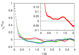
(a)  (b)

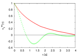
Figure 3.8: Velocity autocorrelation function Eq. (3.5) for bumblebee velocities $v_{y}$ parallel to the wall at three different stages of the experiment shown in Fig. 3.6: (a) Experimental results for stage 1 without spiders (red), 2 under predation threat (green), and 3 under threat a day after the last encounter with the spiders (blue). The data show the effect of the presence of spiders on the bumblebee flights. The inset presents the resampled autocorrelation for the spider-free stage in the region where the correlation differs from the stages with spider models, which confirms that the positive autocorrelations are not a numerical artifact. (b) Theoretical results for the same quantity obtained from numerically solving the Langevin equation (3.6) by switching off (red triangles, upper line) / on (green circles, lower line) a repulsive force modeling the interaction of a bumblebee with a spider. These results qualitatively reproduce the experimental findings in (a).

Figure 3.8(a) shows the bumblebee velocity autocorrelations defined by Eq. (3.5) for all three stages of the experiment. While for the spider-free stage the correlations remain positive for rather long times, in the presence of spiders they quickly become negative. This means that the velocities are on average anti-parallel to each other, or anti-correlated. In terms of flights, when predators are not present the bumblebees thus fly on average more often in the same direction for short times while in the presence of predators on average they often reverse their flight directions for shorter times. This result can be biologically understood as reflecting a more careful search under predation threat: When no predators are present, the bumblebees forage with more or less direct flights from flower to flower. However, under threat the bumblebees change their direction more often in their search for food sources, rejecting flowers with spiders. Mathematically this means that the distributions of velocities remain the same, irrespective of whether predators are present or not, while the topology, i.e., the shape of the bumblebee trajectories changes profoundly being on average more ‘curved’.

In order to theoretically reproduce these changes we model the dynamics of $v_{y}$ by a Langevin equation Reif . It may be called Newton’s Law of stochastic physics, as it is based on Newton’s Second Law: $F=m\cdot a$, where $m$ is the mass of a tracer particle in a fluid moving with acceleration $a=d^{2}x/dt^{2}$ at position $x(t)$ (for sake of simplicity we restrict ourselves to one dimension). To model the interaction of the tracer particle with the surrounding fluid, the force $F$ on the left hand side is written as a sum of two different forces, $F=F_{S}+F_{b}$: a friction term $F_{S}=-\eta v=-\eta\;dx/dt$ with Stokes friction coefficient $\eta$, which models the damping by the surrounding fluid; and another term $F_{b}$ that mimicks the microscopic collisions of the tracer particle with the surrounding fluid particles, which are supposed to be much smaller than the tracer particle. The latter interaction is modeled by a stochastic force $\xi(t)$ of the same type as we have described in Sec. 3.3.5 for which here one takes Gaussian white noise. Interestingly, the stochastic Langevin equation can be derived from first principles starting from Newton’s microscopic equations of motion for the full deterministic dynamical system of a tracer particle interacting with a fluid consisting of many particles Kla06 .

At first view it may look strange to apply such an equation for modeling the motion of a biological organism. However, for a bumblebee the force terms may simply be reinterpreted: While the friction term still models the loss of velocity due to the surrounding air during a flight, the stochastic force term now mimicks both the force actively exerted by the bumblebee to perform a flight and the randomness of these flights due to the surrounding air, and to sudden changes of direction by the bumblebee itself. In addition, for our experiment we need to model the interaction with predators by a third force term. This leads to Eq. (20) stated in Chap. 2, which for bumblebee velocities $v_{y}$ we rewrite as

$$\frac{dv_{y}(t)}{dt}=-\eta v_{y}(t)-\frac{dU(y(t))}{dy}+\xi(t)\>.$$ (3.6)

Here we have combined the mass $m$ with the other terms on the right hand side. The term $F_{i}=-dU(y(t))/dy$ with potential $U$ mimics an interaction between bumblebee and spider, which can be switched on or off depending on whether a spider is present or not. Data analysis shows that this force is strongly repulsive LICCK12 . Computing the velocity autocorrelation function Eq. (3.5) by solving the above equation numerically for a suitable choice of a repulsive force qualitatively reproduces a change from positive to negative correlations when switching on the repulsive force, see Fig. 3.8(b).

These results demonstrate that velocity correlations can contain crucial information for understanding foraging dynamics, here in the form of highly non-trivial correlation decay emerging from the interaction of a forager with predators. This experiment could not test the LSH, as the mathematical assumptions on its validity were not fulfilled. However, conceptually these results are in line with the idea underlying the LEH: Theoretically the interaction between forager and environment was modeled by a repulsive force, to be switched on in the presence of predators, which qualitatively reproduced the experimental results. Together with the spatially intermittent dynamics when approaching the food sources as discussed before, these findings illustrate a complex spatio-temporal adjustment of the bumblebees both to the presence of food sources and predators. This is in sharp contrast to the scale-free dynamics singled out by the LFH.

Of course, modeling bumblebee flights by a Langevin equation like Eq. (3.6) ignores many fine details. A more sophisticated model that reproduces bumblebee flights far away from the flowers more appropriately has been constructed in Ref. LCK13 based on the same data as discussed above.

3.5 Lévy flights embedded in Movement Ecology

The main theme of our chapter was the question posed to the end of the introduction: Can search for food by biological organisms be understood by mathematical modeling? While about a century ago this question was answered by Karl Pearson in terms of simple random walks yielding Brownian motion, about two decades ago the LFH gave a different answer by proposing Lévy motion to be optimal for foraging success, under certain conditions. Discussing experimental results testing it, we arrived at a finer distinction between two different types of LFHs: The LSH captured the essence of the original LFH by stating that under certain conditions Lévy flights represent an optimal search strategy for finding targets. In contrast the LEH stipulates that Lévy flights may emerge from the interaction between a forager and possibly scale-free food source distributions. A weaker version of these different hypotheses we coined the LFP, which suggests to look for power laws in the probability distributions of move step lengths of foraging organisms. An even weaker guiding principle derived from it is to assume that the foraging dynamics of biological organisms can generally be understood by analyzing step length probability distributions alone. We thus have a hierarchy of different LFHs that have all been tested in the literature, in one way or the other.

By elaborating on experimental results, exemplified by selected publications, we outlined a number of problems when testing the different LFHs: miscommunication between theorists and experimentalists leading to incorrect data analysis; the difficulties to mathematically model a specific foraging situation by giving proper credit to all relevant biological details; and problems with an adequate statistical data analysis that really tests for the theory by which it was motivated. We highlighted that there are alternative stochastic processes, such as intermittent search strategies, that may outperform Lévy strategies under certain conditions, or at least lead to similar results, such that it may be hard to clearly distinguish them from Lévy motion. We also discussed an experiment on foraging bumblebees, which showed that relevant information to understand a biological foraging process may not always be contained in the probability distributions that are at the heart of all versions of the LFH. These experimental results suggested that biological organisms may rather perform a complex spatio-temporal adjustment to optimize their search for food sources, which results in different dynamics on different spatio-temporal scales. This is at variance to Lévy motion, which by definition is scale-free.

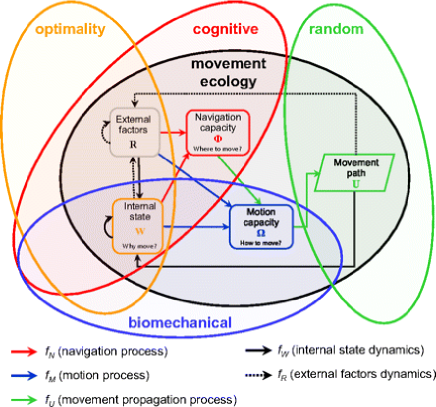
Figure 3.9: Sketch of the Movement Ecology Paradigm: It cross-links four other existing paradigms representing different scientific disciplines, which describe specific aspects of the movements of biological organisms. The aim is to mathematically model the dynamics emerging from the interplay between these different fields by an equation like Eq. (3.7); from Nath08 , copyright (2008) National Academy of Sciences, U.S.A.

However, these results are well in line with another, more general approach to understand the movements of biological organisms, called the Movement Ecology Paradigm Nath08 : This theory aims at more properly embedding the movements of biological organisms into their biological context as shown in Fig. 3.9. In this figure, the theory centered around the LFH is rather represented by the region labeled ‘random’, which focuses on analyzing movement paths only. However, movement paths of organisms cannot properly be understood without embedding them into their biological context: They are to quite some extent determined by the cognitive abilities of the organisms and their biomechanical abilities, see the respective two further regions in this diagram. Indeed, only on this basis the question about optimality may be asked, cf. the fourth region in this diagram, which here is rather understood in a biological sense than as purely mathematical efficiency. Physicists and mathematicians are used to think of diffusive spreading, which underlies foraging, primarily in terms of moving point particles; however, living biological organisms are not point particles but interact with the surrounding world in a very different manner. The aim of this approach is to model the interaction between the four core fields sketched in this diagram by a state space approach. This requires to identify relevant variables, cf. the diagram, by establishing functional relationships between them in form of an equation

$${\bf u}_{t+1}=F({\bm{\Omega}},{\bm{\Phi}},{\bf r}_{t},{\bf w}_{t},{\bf u}_{t})\>,$$ (3.7)

where ${\bf u}_{t}$ is the location of an organism at time $t$. A simple, boiled-down example of such an equation is the Langevin equation Eq. (3.6) that we proposed to describe bumblebee flights under predation threat. Here $du_{t+1}/dt=v_{y}(t)$ and the potential term is related to the variable $r_{t}$ above while all the other variables are ignored.

3.6 Conclusions

The discussion about the LFH is still very much ongoing. As an example we refer to research on movements of mussels, where experimental measurements seemed to suggest that Lévy movement accelerates pattern formation dJWH11 ; however, see the discussion that emerged about these findings as comments and replies to the above paper, which mirrors our discussion in the previous sections. A second example is the debate about a recent review by Andy Reynolds Reyn15 , in which yet another new version of a LFH was suggested; again, see all the respective comments and the authors’ reply to them. While these two articles are in support of the LFH, we refer to a recent review by Graham Pyke Pyke15 as an example of a more critical appreciation of it.

We conclude that one needs to be rather careful with following power law hypotheses, or paradigms, for data analysis, here applied to the problem of understanding the search for food by biological organisms. These laws are very attractive because of their simplicity, and because in certain physical situations they represent underlying universalities. While they clearly have their justification in specific settings, these are rather simplistic concepts that ignore many details of the biological situation at hand. This can cause problems when biological processes are more complex. What we have outlined represents not an entirely new scientific lesson; see, e.g., the discussion about power laws in self-organized criticality. On the other hand, the LFH did pioneer a new way of thinking that goes beyond applying simple traditional random walk schemes to understand biological foraging.

Financial support of this research by the MPIPKS Dresden and the Office of Naval Research Global is gratefully acknowledged.

References

- (1) M. Chupeau, O. Bénichou, R. Voituriez, Nat. Phys. 11, 844 (2015)
- (2) R. Klages, Physik Journal 14, 22 (2015)
- (3) T. Harris, E. Banigan, D. Christian, C. Konradt, E.T. Wojno, K. Norose, E. Wilson, B. John, W. Weninger, A. Luster, Nature 486, 545 (2012)
- (4) G. Ramos-Fernández, J.L. Mateos, O. Miramontes, G. Cocho, H. Larralde, B. Ayala-Orozco, Behav. Ecol. Sociobiol. 55, 223 (2003)
- (5) M. Shlesinger, Nature 443, 281 (2006)
- (6) L. Stone, Theory of Optimal Search, 2nd edn. (Informs, Hanover, MD, 2007)
- (7) R. Nathan, W.M. Getz, E. Revilla, M. Holyoak, R. Kadmon, D. Saltz, P.E. Smouse, Proc. Natl. Acad. Sci. 105, 19052 (2008)
- (8) V. Méndez, D. Campos, F. Bartumeus, Stochastic Foundations in Movement Ecology. Springer series in synergetics (Springer, Berlin, 2014)
- (9) G. Viswanathan, V. Afanasyev, S. Buldyrev, E. Murphy, P. Prince, H. Stanley, Nature 381, 413 (1996)
- (10) G. Viswanathan, S. Buldyrev, S. Havlin, M. da Luz, E. Raposo, H. Stanley, Nature 401, 911 (1999)
- (11) A. Edwards, R. Phillips, N. Watkins, M. Freeman, E. Murphy, V. Afanasyev, S. Buldyrev, M. da Luz, E. Raposo, H. Stanley, G. Viswanathan, Nature 449, 1044 (2007)
- (12) D. Sims, E. Southall, N. Humphries, G.C. Hays, C.J.A. Bradshaw, J.W. Pitchford, A. James, M.Z. Ahmed, A.S. Brierley, M.A. Hindell, D. Morritt, M.K. Musyl, D. Righton, E.L.C. Shepard, V.J. Wearmouth, R.P. Wilson, M.J. Witt, J.D. Metcalfe, Nature 451, 1098 (2008)
- (13) N. Humphries, N. Queiroz, J. Dyer, N. Pade, M. Musy, K. Schaefer, D. Fuller, J. Brunnschweiler, T. Doyle, J. Houghton, G. Hays, C. Jones, L. Noble, V. Wearmouth, E. Southall, D. Sims, Nature 465, 1066 (2010)
- (14) F. Lenz, T.C. Ings, L. Chittka, A.V. Chechkin, R. Klages, Phys. Rev. Lett. 108, 098103/1 (2012)
- (15) F. Lenz, A.V. Chechkin, R. Klages, PLoS ONE 8, e59036 (2013)
- (16) M. Shlesinger, G. Zaslavsky, J. Klafter, Nature 363, 31 (1993)
- (17) G. Viswanathan, M. da Luz, E. Raposo, H. Stanley, The Physics of Foraging (Cambridge University Press, Cambridge, 2011)
- (18) K. Pearson, Biometric ser. 3, 54 (1906)
- (19) R. Klages, G. Radons, I. Sokolov (eds.), Anomalous transport (Wiley-VCH, Berlin, 2008)
- (20) V. Zaburdaev, S. Denisov, J. Klafter, Rev. Mod. Phys. 87, 483 (2015)
- (21) M. Buchanan, Nature 453, 714 (2008)
- (22) M. de Jager, F.J. Weissing, P.M.J. Herman, B.A. Nolet, J. van de Koppel, Science 332, 1551 (2011)
- (23) G. Pyke, Meth. Ecol. Evol. 6, 1 (2015)
- (24) A. Reynolds, Phys. Life Rev. 14, 59 (2015)
- (25) O. Bénichou, C. Loverdo, M. Moreau, R. Voituriez, Rev. Mod. Phys. 83, 81 (2011)
- (26) A. James, J.W. Pitchford, M.J. Plank, Bull. Math. Biol. 72, 896 (2009)
- (27) N. Humphries, H. Weimerskirch, N. Queiroz, E. Southall, D. Sims, PNAS 109, 7169 (2012)
- (28) R. Metzler, J. Klafter, Phys. Rep. 339, 1 (2000)
- (29) J. Klafter, I. Sokolov, First Steps in Random Walks: From Tools to Applications (Oxford University Press, Oxford, 2011)
- (30) R. Metzler, J. Klafter, J. Phys. A: Math. Gen. 37, R161 (2004)
- (31) T.C. Ings, L. Chittka, Current Biology 18, 1520 (2008)
- (32) R. Klages, Microscopic chaos, fractals and transport in nonequilibrium statistical mechanics, Advanced Series in Nonlinear Dynamics, vol. 24 (World Scientific, Singapore, 2007)
- (33) F. Reif, Fundamentals of statistical and thermal physics (McGraw-Hill, Auckland, 1965)
Index
- albatross §3.2.1
- Brownian motion §3.2.2
- bumblebee §3.4
- central limit theorem §3.1, §3.3.5
- correlation §3.4.2
- covariance §3.4.2
-
diffusion
- anomalous §3.3.5
- emergence item 1, §3.5
- foraging §3.1, §3.2.2, §3.4.1
- intermittency §3.3.4
- Langevin equation §3.4.2
- Lévy §3.1
- Markov process §3.3.5
- memory §3.4.2
- movement ecology Figure 3.9, §3.1, §3.5
- operations research §3.1
- power law §3.1, §3.3.2, §3.6
-
random walk §3.3.5
- continuous time §3.3.5
- search §3.1, §3.3.4, §3.5
- state space §3.5
- subdiffusion §3.3.5
- superdiffusion §3.3.5
- velocity autocorrelation function Figure 3.8, §3.4.2