Multimodal Sparse Bayesian Dictionary Learning

Abstract

This paper addresses the problem of learning dictionaries for multimodal datasets, i.e. datasets collected from multiple data sources. We present an algorithm called multimodal sparse Bayesian dictionary learning (MSBDL). MSBDL leverages information from all available data modalities through a joint sparsity constraint. The underlying framework offers a considerable amount of flexibility to practitioners and addresses many of the shortcomings of existing multimodal dictionary learning approaches. In particular, the procedure includes the automatic tuning of hyperparameters and is unique in that it allows the dictionaries for each data modality to have different cardinality, a significant feature in cases when the dimensionality of data differs across modalities. MSBDL is scalable and can be used in supervised learning settings. Theoretical results relating to the convergence of MSBDL are presented and the numerical results provide evidence of the superior performance of MSBDL on synthetic and real datasets compared to existing methods.

I Introduction

Due to improvements in sensor technology, acquiring vast amounts of data has become relatively easy. Given the ability to harvest data, the task becomes how to extract relevant information from the data. The data is often multimodal, which introduces novel challenges in learning from it. Multimodal dictionary learning has become a popular tool for fusing multimodal information [1, 2, 3, 4, 5].

Let $L$ and $J$ denote the number of data points for each modality and number of modalities, respectively. Let $Y_{j}=\begin{bmatrix}y_{j}^{1}&\cdots&y_{j}^{L}\end{bmatrix}\in\mathbb{R}^{N_{j}\times L}$ denote the data matrix for modality $j$, where $y_{j}^{i}$ denotes the $i$’th data point for modality $j$. We use uppercase symbols to denote matrices and lowercase symbols to denote the corresponding matrix columns. The multimodal dictionary learning problem consists of estimating dictionaries $D_{j}\in\mathbb{R}^{N_{j}\times M_{j}}$ given data ${Y_{j}}$ such that $Y_{j}\approx D_{j}X_{j}\;\forall j.$ We focus on overcomplete dictionaries because they are more flexible in the range of signals they can represent [6]. Since $y_{j}^{i}$ admits an infinite number of representations under overcomplete $D_{j}$, we seek sparse $x_{j}^{i}$ [7].

Without further constraints, the multimodal dictionary learning problem can be viewed as $J$ independent unimodal problems. To fully capture the multimodal nature of the problem, the learning process must be adapted to encode the prior knowledge that each set of points $\bm{y^{i}}=\left\{y_{j}^{i}\right\}_{j\in[J]}$ is generated by a common source which is measured $J$ different ways, where $[J]=\left\{1,\cdots,J\right\}$. For any variable $x$, $\bm{x}$ denotes $\left\{x_{j}\right\}_{j\in[J]}$. For instance, in [8], low and high resolution image patches are modelled as $y_{1}^{i}$ and $y_{2}^{i}$, respectively, and the association between $y_{1}^{i}$ and $y_{2}^{i}$ is enforced by the constraint $x_{1}^{i}=x_{2}^{i}$. The resulting multimodal dictionary learning problem, referred to here as $\ell_{1}$DL, is to solve [9]

$$\operatorname*{arg\,min}_{\tilde{D},X}\left\|{\tilde{Y}}-{\tilde{D}}{X}\right\|_{F}^{2}+ \lambda\left\|X\right\|_{1}$$ (1)

$$\tilde{Y}=\begin{bmatrix}Y_{1}^{T}&\cdots&Y_{J}^{T}\end{bmatrix}^{T}, \;\tilde{D}=\begin{bmatrix}D_{1}^{T}&\cdots&D_{J}^{T}\end{bmatrix}^{T},$$

where $\left\|\cdot\right\|_{F}$ is the Frobenius norm, $\left\|X\right\|_{1}=\sum_{i\in[L]}\left\|x^{i}\right\|_{1}$, and the $\ell_{1}$-norm is used as a convex proxy to the $\ell_{0}$ sparsity measure. In a classification framework, (1) can be viewed as learning a multimodal feature extractor, where the optimizer is the multimodal representation of $\bm{y^{i}}$ that is fed into a classifier [1, 10, 2]. There are $4$ significant deficiencies associated with using $\ell_{1}$DL for multimodal dictionary learning. In fact, all existing approaches suffer from one of more of the following:

1. While using the same sparse code for each modality establishes an explicit relationship between the dictionaries for each modality, the same coefficient values may not be able to represent different modalities well.

2. Some data modalities are often less noisy than others and the algorithm should be able to leverage the clean modalities to learn on the noisy ones. Since (1) constrains $\lambda$ to be the same for all modalities, it is unclear how the learning algorithm can incorporate prior knowledge about the noise level of each modality.

3. The formulation in (1) constrains $M_{j}=M\;\forall j$, for some $M$. Since dimensionality can vary across modalities, it is desirable to allow $M_{j}$ to vary.

4. The choice of $\lambda$ is central to the success of approaches like (1). If $\lambda$ is chosen too high, the reconstruction term is ignored completely, leading to poor dictionary quality. If $\lambda$ is chosen too low, the sparsity promoting term is effectively eliminated from the objective function. Extensive work has been done to approach this hyperparameter selection problem from various angles. Two popular approaches include treating the hyperparameter selection problem as an optimization problem of its own [11, 12] and grid search, with the latter being the prevailing strategy in the dictionary learning community [9, 13]. In either case, optimization of $\lambda$ involves evaluating (1) at various choices of $\lambda$, which can be computationally intensive and lead to suboptimal results in practice. For some of the successful multimodal dictionary learning algorithms [5, 4], where each modality is associated with at least one hyperparameter, grid search becomes prohibitive since the search space grows exponentially with $J$. For more details, see Section IV-C, specifically Table IV and Fig. 5, for a comparison of competing algorithms in terms of computational complexity when grid-search hyperparameter tuning is taken into account.

Next, we review relevant works from the dictionary learning literature, highlighting each method’s benefits and drawbacks in light of D1-D4. Table I summarizes where competing algorithms fall short in terms of D1-D4.

In past work, $M_{j}=M\;\forall j$, thus exhibiting D3. One of the seminal unimodal dictionary learning algorithms is K-SVD, which optimizes [7]

$$\operatorname*{arg\,min}_{D,\;\left\{\left\|x^{i}\right\|_{0}\leq s\right\}_{i\in[L]}}\left\|Y-DX\right\|_{F}^{2},$$ (2)

where $s$ denotes the desired sparsity level and modality subscripts have been omitted for brevity. The K-SVD algorithm proceeds in a block-coordinate descent fashion, where $D$ is optimized while holding $X$ fixed and vice-versa. The update of $X$ involves a greedy $\ell_{0}$ pseudo-norm minimization procedure [14]. In a multimodal setting, K-SVD can be naively adapted, where $Y$ is replaced by $\tilde{Y}$ and $D$ by $\tilde{D}$ in (2), as in (1).

One recent approach, referred to here as Joint $\ell_{0}$ Dictionary Learning (J$\ell_{0}$DL), builds upon K-SVD for the multimodal dictionary learning problem and proposes to solve [4]

$$\operatorname*{arg\,min}_{\left\{\left\{\chi_{j}^{i}=\chi^{i}\right\}_{j\in[J]},|\chi^{i}|\leq s\right\}_{i\in[L]}}\sum_{j=1}^{J}\lambda_{j}\left\|Y_{j}-D_{j}X_{j}\right\|_{F}^{2}$$ (3)

where $\chi_{j}^{i}$ denotes the support of $x_{j}^{i}$. The J$\ell_{0}$DL algorithm tackles D1-D2 by establishing a correspondence between the supports of the sparse codes for each modality and by allowing modality specific regularization parameters, which allow for encoding prior information about the noise level of $y_{j}^{i}$. On the other hand, J$\ell_{0}$DL does not address D3 and presents even more of a challenge than $\ell_{1}$DL with respect to D4 since the size of the grid search needed to find $\bm{\lambda}$ grows exponentially with $J$. Another major drawback of J$\ell_{0}$DL is that, since (3) has an $\ell_{0}$ type constraint, solving it requires a greedy algorithm which can produce poor solutions, especially if some modalities are much noisier than others [15].

The multimodal version of (1), referred to here as Joint $\ell_{1}$ DL (J$\ell_{1}$DL), seeks [16]

$$\operatorname*{arg\,min}_{\bm{D},\bm{X}}\frac{1}{2}\sum_{i\in[L],j\in[J]}\left\|y_{j}^{i}-D_{j}x_{j}^{i}\right\|_{2}^{2}+\lambda\sum_{i\in[L]}\left\|\Pi^{i}\right\|_{12}$$ (4)

where $\Pi^{i}=\begin{bmatrix}x_{1}^{i}&\cdots&x_{J}^{i}\end{bmatrix}$, $\left\|\Pi^{i}\right\|_{12}=\sum_{m\in[M]}\left\|\Pi^{i}[m,:]\right\|_{2},$ and $\Pi^{i}[m,:]$ denotes the $m$’th row of $\Pi^{i}$. The $\ell_{12}$-norm in (4) promotes row sparsity in $\Pi^{i}$, which promotes $\bm{x^{i}}$ that share the same support. Interestingly, regularizers which promote common support amongst variables appear in a wide range of works, including graphical model identification [17, 18]. Like all of the previous approaches, J$\ell_{1}$DL adopts a block-coordinate descent approach to solving (4), where an alternating direction method of multipliers algorithm is used to compute the sparse code update stage [19]. While J$\ell_{1}$DL makes progress toward addressing D1, it does so at the cost of sacrificing the hard constraint that $\bm{x^{i}}$ share the same support. The authors of [16] attempt to address D2 by relaxing the constraint on the support of $\bm{x^{i}}$ even more, but we will not study this approach here because it moves even further from the theme of this work. In addition, J$\ell_{1}$DL does not address D3-D4. Although D4 is not as serious of an issue for J$\ell_{1}$DL as for J$\ell_{0}$DL because J$\ell_{1}$DL requires tuning a single hyperparameter, D3 limits the usefulness of J$\ell_{1}$DL in situations where the observed modalities are drastically different in type and cardinality, i.e. text and images.

One desirable property of dictionary learning approaches is that they be scalable with respect to the size of the dictionary as well as the dataset. When $L$ becomes large, the algorithm must be able to learn in a stochastic manner, where only a subset of the data samples need to be processed at each iteration. Stochastic learning strategies have been studied in the context of $\ell_{1}$DL [9, 20] and J$\ell_{1}$DL [16], but not for K-SVD or J$\ell_{0}$DL. Likewise, the algorithm should be able to accommodate large $N_{j}$.

	MSBDL		J$\ell_{1}$DL	J$\ell_{0}$DL	$\ell_{1}$DL	KSVD
	Proposed	[5]
D1					✓	✓
D2			✓		✓	✓
D3		✓	✓	✓	✓	✓
D4		✓	✓	✓	✓	✓

TABLE I: Deficiencies that existing dictionary learning algorithms suffer from.

When the dictionary learning algorithm is to be used as a building block in a classification framework, class information can be incorporated within the learning process. In a supervised setting, the input to the algorithm is $\left\{\bm{Y},H\right\}$, where $H=\begin{bmatrix}h^{1}&\cdots&h^{L}\end{bmatrix}\in\mathbb{B}^{C\times L}$ is the binary class label matrix for the dataset and $C$ is the number of classes. Each $h^{i}$ is the label for the $i$’th data point in a one-of-$C$ format. This type of dictionary learning is referred to as task-driven [16, 20], label consistent [13], or discriminative [21] and the goal is to learn a dictionary $D_{j}$ such that $x_{j}^{i}$ is indicative of the class label. For instance, discriminative K-SVD (D-KSVD) optimizes [21]

$$\operatorname*{arg\,min}_{D,W,\left\{\left\|x^{i}\right\|_{0}\leq s\right\}_{i\in[L]}}\left\|Y-DX\right\|_{F}^{2}+\lambda_{su}\left\|H-WX\right\|_{F}^{2}$$ (5)

where $W$ can be viewed as a linear classifier for $x^{i}$.

Task-driven $\ell_{1}$DL (TD-$\ell_{1}$DL) optimizes [20]

$$\operatorname*{arg\,min}_{D,W}E_{x}\left[l_{su}(h,W,x^{*}(y,D)\right]+\nu\left\|W\right\|_{F}^{2}$$ (6)

where $E_{x}[\cdot]$ denotes the expectation with respect to $p\left(x\right)$, $l_{su}(\cdot)$ denotes the supervised loss function, $x^{*}(y,D)$ denotes the solution of (1) with the dictionary fixed to $D$, and the last term provides regularization on $W$ to avoid over-fitting.

Task-driven J$\ell_{1}$DL (TD-J$\ell_{1}$DL) optimizes [16]

$$\operatorname*{arg\,min}_{\bm{D},\bm{W}}E_{\bm{x}}\left[\sum_{j\in[J]}l_{su}(h_{j},W_{j},x_{j}^{*}(y_{j},D_{j})\right]+\nu\sum_{j\in[J]}\left\|W_{j}\right\|_{F}^{2}$$

where $x_{j}^{*}(y_{j},D_{j})$ denotes the $j$’th modality sparse code in the optimizer of (4) with fixed dictionaries.

I-A Contributions

We present the multimodal sparse Bayesian dictionary learning algorithm (MSBDL). MSBDL is based on a hierarchical sparse Bayesian model, which was introduced in the context of Sparse Bayesian Learning (SBL) [22, 23, 24] as well as dictionary learning [22], and has since been extended to various structured learning problems [25, 26, 27]. We presented initial work on this approach in [5], where we made some progress towards tackling D1-D2. Here, we go beyond our preliminary work in a number of significant ways, which are summarized in Table II. We address D1-D2 to a fuller extent by offering scalable and task-driven variants of MSBDL. More importantly, we tackle D3-D4, where our solution to D4 is crucial to the ability of MSBDL to address D1 and resolves a major hyperparameter tuning issue in [5]. By resolving D3, the present work represents a large class of algorithms that contains [5] as a special case. This point is depicted in Fig. 1, which provides a visualization of the types of models and variable interactions that can be learned by each of the competing algorithms.

In summary:

1. We extend MSBDL to address D3. To the best of our knowledge, MSBDL is the first dictionary learning algorithm capable of learning differently sized dictionaries.

2. We extend MSBDL to the task-driven learning scenario.

3. We present scalable versions of MSBDL.

4. We optimize algorithm hyperparameters during learning, obviating the need for grid search, and conduct a theoretical analysis of the approach.

5. We show that multimodal dictionary learning offers provable advantages over unimodal dictionary learning.

Figure 1: Modeling capacity of proposed algorithm compared to existing works.

	Proposed	[5]
Scalable	✓
Task-driven extension	✓
Solves D3	✓
Solves D4	✓

TABLE II: Comparison of proposed MSBDL variant with [5].

I-B On the Motivation of this Work

Consider the scenario depicted in Fig. 2. The solid rectangles represent learning models 1 and 2, corresponding to modalities 1 and 2, respectively, independently of each other. The intuition behind this work is that model 2 can be improved by performing learning in a joint fashion, where information flows between models 1 and 2, as depicted by the dotted shapes in Fig. 2. The experimental and theoretical results reported in this paper all serve as evidence for the ability of MSBDL to leverage all available data sources to learn models for each modality that are superior to ones that could be found if learning was done independently. As such, the aims of this work are, in some sense, tangential to works like [16], where the goal is more to learn an information fusion scheme and less to learn superior models for each modality.

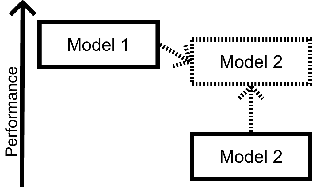
Figure 2: Visualization of high level problem motivation.

II Proposed Approach

Figure 3: Graphical model for two modality MSBDL.

The graphical model for MSBDL is shown in Fig. 3. The signal model is given by

$${y_{j}}={D_{j}x_{j}}+{v_{j}},\;\;{v_{j}}\sim\mathsf{N}\left(0,\sigma_{j}^{2}{\mathsf{I}}\right)$$ (7)

where $\mathsf{N}(\cdot)$ denotes a Gaussian distribution and the noise variance is allowed to vary among modalities. In order to promote sparse $x_{j}^{i}$, we assume a Gaussian Scale Mixture (GSM) prior on each element of ${x_{j}}$ [23, 24, 28, 29]. The GSM prior is a popular class of distributions whose members include many sparsity promoting priors, such as the Laplacian and Student’s-t [23, 24, 28, 29, 30, 31]. The remaining task is to specify the conditional density of ${x_{j}}$ given ${\gamma}$. One option is to use what we refer to as the one-to-one prior [5]:

$$p\left(x_{j}|\gamma\right)=\prod_{m\in[M]}p\left(x_{j}[m]|\gamma[m]\right)=\prod_{m\in[M]}\mathsf{N}\left(0,\gamma[m]\right)$$ (8)

where $x_{j}[m]$ denotes the $m$’th element of $x_{j}$ and the choice of $p(\gamma[m])$ determines the marginal density of ${x_{j}[m]}$. We assume a non-informative prior on ${\gamma_{j}[m]}$ [23]. As will be shown in Section II-B, the conditional distribution in (8) represents a Bayesian realization of the constraint that $\bm{x}$ share the same support. The prior in (8) still constrains $M_{j}=M\;\forall j$, but this restriction will be lifted in Section V. When $J=1$, this model is identical to the one used in [22].

II-A Inference Procedure

We adopt an empirical Bayesian inference strategy to estimate $\theta=\left\{\bm{D},\left\{\gamma^{i}\right\}_{i\in[L]}\right\}$ by optimizing [32]

$$\operatorname*{arg\,max}_{\theta} \log p\left(\bm{Y}|\theta\right)=\operatorname*{arg\,max}_{\theta}\sum_{j\in[J]}\log p\left({Y_{j}}|\theta\right)$$ (9)

$$p\left(\bm{Y}|\theta\right) =\prod_{i\in[L],j\in[J]}p\left(y_{j}^{i}|\theta\right),p\left(y_{j}^{i}|\theta\right)=\mathsf{N}(0,\Sigma_{y}^{i})$$ (10)

$$\Sigma_{y,j}^{i} =\sigma_{j}^{2}\mathsf{I}+D_{j}\Gamma^{i}D_{j}^{T},\;\;\Gamma^{i}=\text{diag}(\gamma^{i}).$$ (11)

We use Expectation-Maximization (EM) to maximize (9), where $\left\{\bm{X},\bm{Y},\theta\right\}$ and $\bm{X}$ are treated as the complete and nuisance data, respectively [33]. At iteration $t$, the E-step computes $Q\left(\theta,\theta^{t}\right)=\left\langle\log p\left(\bm{Y},\bm{X},\bm{D},\left\{\gamma^{i}\right\}_{i\in[L]}\right)\right\rangle$, where $\langle\cdot\rangle$ denotes the expectation with respect to $p\left(\bm{X}|\bm{Y},\theta^{t}\right)$, and $\theta^{t}$ denotes the estimate of $\theta$ at iteration $t$. Due to the conditional independence properties of the model, the posterior factors over $i$ and

$$p\left(x_{j}^{i}|y_{j}^{i},\theta\right) =\mathsf{N}\left(\mu_{j}^{i},\Sigma_{x,j}^{i}\right)$$ (12)

$${\Sigma}_{x,j}^{i} =\left({\sigma_{j}^{-2}{D}_{j}^{T}{D}_{j}+\left({\Gamma^{i}}\right)^{-1}}\right)^{-1}$$ (13)

$${\mu}_{j}^{i} =\sigma_{j}^{-2}{\Sigma}_{x,j}^{i}{D}_{j}^{T}y_{j}^{i}.$$ (14)

In the M-step, $Q\left(\theta,\theta^{t}\right)$ is maximized with respect to $\theta$. In general, the M-step depends on the choice of $p\left(\bm{x}|\gamma\right)$. For the choice in (8), the M-step becomes

$$\left(\gamma^{i}[m]\right)^{t+1} =J^{-1}{\sum_{j=1}^{J}{\Sigma}_{x,j}^{i}[m,m]+\left({\mu}_{j}^{i}[m]\right)^{2}}$$ (15)

$$D_{j}^{t+1} =Y_{j}{U}_{j}^{T}\left({{U}_{j}{U}_{j}^{T}+\sum_{i\in[L]}{\Sigma}_{x,j}^{i}}\right)^{-1}$$ (16)

$$U_{j} =\begin{bmatrix}\mu_{j}^{1}&\cdots&\mu_{j}^{L}\end{bmatrix}.$$ (17)

II-B How does MSBDL solve deficiency D1?

One consequence of the GSM prior is that many of the elements of $\gamma^{i}$ converge to $0$ during inference [24]. When $\gamma^{i}[m]=0$, $p\left(x_{j}^{i}[m]|y_{j}^{i},\gamma^{i}\right)$ reduces to $\delta\left(x_{j}[m]\right)$ for all $j$, where $\delta(\cdot)$ denotes the Dirac-delta function [24]. Since the only role of $\bm{x}$ in the inference procedure is in the E-step, where we take the expectation of the complete data log-likelihood with respect to $p\left(x_{j}^{i}|y_{j}^{i},\gamma^{i}\right)$, the effect of having $p\left(x_{j}^{i}[m]|y_{j}^{i},\gamma^{i}\right)=\delta\left(x_{j}^{i}[m]\right)$ is that the E-step reduces to evaluating the complete data log-likelihood at $x_{j}^{i}[m]=0,\forall j$. Therefore, upon convergence, the proposed approach exhibits the property that $\bm{x^{i}}$ share the same support.

II-C Connection to J$\ell_{1}$DL

Suppose that the conditional distribution in (8) is used with ${\gamma[m]}\sim\mathsf{Ga}\left({J}/{2},1\right)\;\forall m$, where $\mathsf{Ga}(\cdot)$ refers to the Gamma distribution. It can be shown that [34]

$$p\left(\bm{x^{i}}\right)=c\prod_{m\in[M]}K_{0}\left(\left\|\begin{bmatrix}x_{1}^{i}[m]&\cdots&x_{J}^{i}[m]\end{bmatrix}\right\|_{2}\right),$$

where $c$ is a normalization constant and $K_{0}(\cdot)$ denotes the modified Bessel function of the second kind and order $0$. For large $x$, $K_{0}(x)\approx{\pi}\exp(-x)/{\sqrt{2\pi x}}$ [35]. In the following, we replace $K_{0}(x)$ by its approximation for purposes of exposition. Under the constraint $\sigma_{j}=0.5\lambda\;\forall j$, the MAP estimate of $\left\{\bm{D},\bm{X}\right\}$ is given by

$$\begin{split}\operatorname*{arg\,min}_{\bm{D},\bm{X}}&\sum_{i\in[L],j\in[J]}\left\|y_{j}^{i}-D_{j}x_{j}^{i}\right\|_{2}^{2}+\lambda\sum_{i\in[L]}\left\|\Pi^{i}\right\|_{12}+\\ &0.5\lambda\sum_{i\in[L],m\in[M]}\log\left\|\Pi^{i}[m,:]\right\|_{2}.\end{split}$$ (18)

This analysis exposes a number of similarities between MSBDL and J$\ell_{1}$DL. If we ignore the last term in (18), J$\ell_{1}$DL becomes the MAP estimator of $\left\{\bm{D},\bm{X}\right\}$ under the one-to-one prior in (8). If we keep the last term in (18), the effect is to add a Generalized Double Pareto prior on the $\ell_{2}$ norm of the rows of $\Pi^{i}$ [31, 36].

At the same time, there are significant differences between MSBDL and J$\ell_{1}$DL. The J$\ell_{1}$DL objective function assumes ${\sigma_{j}}$ is constant across modalities, which can lead to a strong mismatch between data and model when the dataset consists of sources with disparate noise levels. In contrast to J$\ell_{1}$DL, MSBDL enjoys the benefits of evidence maximization [37, 32, 31], which naturally embodies ”Occam’s razor” by penalizing unnecessarily complex models and searches for areas of large posterior mass, which are more informative than the mode when the posterior is not well-behaved.

III Complete Algorithm

So far, it has been assumed that $\bm{\sigma}$ is known. Although it is possible to include $\bm{\sigma}$ in $\theta$ and estimate it within the evidence maximization framework in (9), we experimental observe that $\bm{\sigma}$ decays very quickly and the algorithm tends to get stuck in poor stationary points. An alternative approach is described next. Consider the scenario where $D_{j}$ is known and we seek the MAP estimate of $x_{j}$ given $y_{j},D_{j}$:

$$\operatorname*{arg\,min}_{x_{j}}\left\|y_{j}-D_{j}x_{j}\right\|_{2}^{2}-2\sigma_{j}^{2}\log p\left(x_{j}\right).$$ (19)

The estimator in (19) shows that $\sigma_{j}$ can be thought of as a regularization parameter which controls the trade-off between sparsity and reconstruction error. As such, we propose to anneal $\sigma_{j}$. The motivation for annealing $\sigma_{j}$ is that the quality of $D_{j}$ increases with $t$, so giving too much weight to the reconstruction error term early on can force EM to converge to a poor stationary point.

Let $\sigma_{j}^{0}>\sigma^{\infty}\geq 0,\alpha_{\sigma}<1$, $\tilde{\sigma}_{j}^{t+1}=\max(\sigma^{\infty},\alpha_{\sigma}\sigma_{j}^{t})$. The proposed annealing strategy can then be stated as

$$\sigma_{j}^{t+1}=\begin{cases}\tilde{\sigma}_{j}^{t+1}&\text{ if }\log p\left(Y_{j}|\theta^{t+1},\tilde{\sigma}_{j}^{t+1}\right)>\log p\left(Y_{j}|\theta^{t+1},\sigma_{j}^{t}\right)\\ \sigma_{j}^{t}&\text{ else. }\end{cases}$$ (20)

Although it may seem that we have replaced the task of selecting $\bm{\sigma}$ with that of selecting $\left\{\bm{\sigma^{0}},\alpha_{\sigma},\sigma^{\infty}\right\}$, we claim that the latter is easy to select and provide both theoretical (Section VII) and experimental (Section VIII) validation for this claim. The main benefit of the proposed approach is that it essentially traverses a continuous space of candidate $\bm{\sigma}$ without explicitly performing a grid search, which would be intractable as $J$ grows. The parameter $\sigma^{\infty}$ can be set arbitrarily small and $\bm{\sigma^{0}}$ can be set arbitrarily large. The only recommendation we make is to set $\sigma_{j}^{0}>\sigma_{j^{\prime}}^{0}$ if modality $j$ is a-priori believed to be more noisy than modality $j^{\prime}$.

Section VII studies the motivation for and properties of the annealing strategy in greater detail. In practice, the computation of $p\left(Y_{j}|\theta^{t+1},\tilde{\sigma}_{j}^{t+1}\right)$ is costly because it requires the computation of the sufficient statistics in (11) for all $L$ data points and $J$ modalities. Instead, we replace the condition in (20) by checking whether decreasing $\sigma_{j}$ should increase $p\left(Y_{j}|\theta^{t+1},\sigma^{t}\right)$. This check is performed by checking the sign of the first derivative of $p\left(Y_{j}|\theta^{t+1},\sigma^{t}\right)$, replacing (20) with

$$\sigma_{j}^{t+1}=\begin{cases}\tilde{\sigma}_{j}^{t+1}&\text{ if }{\partial\log p\left(Y_{j}|\theta^{t+1},\sigma_{j}^{t}\right)}/{\partial\sigma_{j}^{t}}<0\\ \sigma_{j}^{t}&\text{ else. }\end{cases}$$ (21)

It can be shown that (21) can be computed essentially for free by leveraging the sufficient statistics computed in the $\theta$ update step. The complete MSBDL algorithm is summarized in Fig. 4. In practice, each ${D_{j}}$ is normalized to unit $\ell_{2}$ column norm at each iteration to prevent scaling instabilities.

1:$\bm{Y},\bm{\sigma^{0}},\sigma^{\infty},\alpha_{\sigma}$

2:while $\bm{\sigma}$ not converged do

3:     while $\bm{D}$ not converged do

4:         for $i\in[L]$ do

5:              Update $\bm{\Sigma_{x}^{i}},\bm{\mu^{i}},\gamma^{i}$ using (13), (14), and (15)

6:         end for

7:         $\left\{\text{ Update }D_{j}\text{ using \eqref{eq:D update} if }\sigma_{j}\text{ not converged}\right\}_{j\in[J]}$

8:     end while

9:     $\left\{\text{Update $\sigma_{j}$ using \eqref{eq:sigma update smart} if $\sigma_{j}$ not converged}\right\}_{j\in[J]}$

10:end while

Figure 4: MSBDL algorithm for the one-to-one prior in (8).

III-A Dictionary Cleaning

We adopt the methodology in [7] and “clean” each ${D_{j}}$ every $T$ iterations. Cleaning $D_{j}$ means removing atoms which are aligned with one or more other atoms and replacing the removed atom with the element of $Y_{j}$ which has the poorest reconstruction under $D_{j}$. A given atom is also replaced if it does not contribute to explaining $Y_{j}$, as measured by the energy of the corresponding row of $U_{j}$.

IV Scalable Learning

When $L$ is large, it is impractical to update the sufficient statistics for all data points at each EM iteration. To draw a parallel with stochastic gradient descent (SGD), when the objective function is a sum of functions of individual data points, one can traverse the gradient with respect to a randomly chosen data point at each iteration instead of computing the gradient with respect to every sample in the dataset. In the dictionary learning community, SGD is often the optimization algorithm of choice because the objective function is separable over each data point [9, 20, 16]. In addition, as $N_{j}$ grows, the computation of the sufficient statistics in (13)-(14) can become intractable. In the following, we propose to address these issues using a variety of modifications of the MSBDL algorithm from Section II. The proposed methods also apply to priors other than the one in (8) .

IV-A Scalability with respect to the size of the dataset

In the following, we present two alternatives to the EM MSBDL algorithm to achieve scalability with respect to $L$. The first proposed approach, referred to here as Batch EM, computes sufficient statistics only for a randomly chosen subset $\phi=\{i^{1},\cdots,i^{L_{0}}\}$ at each EM iteration, where $L_{0}$ denotes the batch size. The M-step consists of updating $\{\gamma^{i}\}_{i\in\phi}$ using (15) and updating $D_{j}$ using (16), with the exception that only the sufficient statistics from $i\in\phi$ are employed.

Another stochastic inference alternative is called Incremental EM, which is reviewed in the Supplementary Material [38]. In the context of MSBDL, Incremental EM is tantamount to an inference procedure which, at each iteration, randomly selects a subset $\phi$ of points and updates the sufficient statistics in (13)-(14) for $i\in\phi$. During the M-step, the hyperparameters $\{\gamma^{i}\}_{i\in\phi}$ are updated. The dictionaries $D_{j}$ are updated using (16), where the update rule depends on sufficient statistics computed for all $L$ data points, only a subset of which have been updated during the given iteration.

	EM Type	$\mu/\Sigma_{x}$	CC	MC
MSBDL	Exact	Exact	$LN^{3}$	$LM^{2}$
MSBDL-1	Incremental	Exact	$L_{0}N^{3}$	$LM^{2}$
MSBDL-2	Incremental	Approximate	$L_{0}N^{2}\lceil N\rceil$	$LM$
MSBDL-3	Batch	Exact	$L_{0}N^{3}$	$L_{0}M^{2}$
MSBDL-4	Batch	Approximate	$L_{0}N^{2}\lceil N\rceil$	$L_{0}M$

TABLE III: CC, MC, $L_{0}$, and $\lceil N\rceil$ denote worst case computational complexity, worst case memory complexity, batch size, and a quantity which is upper-bounded by $N$, respectively.

IV-B Scalability with respect to the size of the dictionary

In order to avoid the inversion of the $N_{j}\times N_{j}$ matrix required to compute (13), we use the conjugate gradient algorithm to compute $\mu_{j}^{i}$ and approximate $\Sigma_{x,j}^{i}$ by

$$\Sigma_{x,j}^{i}\approx\left({diag\left(\sigma^{-2}D_{j}^{T}D_{j}+\left({\Gamma^{i}}\right)^{-1}\right)}\right)^{-1}$$ (22)

where, in this case, $diag(\cdot)$ denotes setting the off-diagonal elements of the input to $0$ [39, 40].

Table III shows a taxonomy of MSBDL algorithms considered using exact or incremental EM and exact or approximate computation of (13)-(14), along with the corresponding worst case computational and memory complexity per EM iteration. The Supplementary Material provides a visualization of the difference between the proposed algorithms.

IV-C Learning complexity

Finally, we consider the learning complexity (LC) of MSBDL, specifically with respect to that of competing approaches, where we define LC to be the (worst-case) computational complexity of running the algorithm and tuning its hyperparameters. In the case of MSBDL, the hyperparameters are learned jointly with the parameters $\theta$, obviating the need for hyperparameter optimization. In the case of J$\ell_{1}$DL, J$\ell_{0}$DL, $\ell_{1}$DL, and K-SVD, we assume that a grid search is performed to estimate the hyperparameters, with a grid spacing of $F$ for each hyperparameter. Analytical results for LC are shown in Table IV and Fig. 5 plots the ratio of LC for competing approaches to that of MSBDL as a function of $J$ for $N=100$, $M=400$, $F=10$, $s=10$, $T=L=1$. For comparison, we also plot the LC of MSBDL-1 with $\lceil N\rceil=1$. The results show that J$\ell_{0}$DL and the MSBDL variant in [5] scale least well with $J$, which can be explained by the fact that both require grid-search to tune $J$ hyperparameters. J$\ell_{1}$DL exhibits worse LC behavior than MSBDL, with the gap between the two methods growing as $J$ increases. Interestingly, MSBDL-1 exhibits the best LC amongst all of the algorithms. The analysis in this section shows that D4 is a serious concern for several existing approaches, especially [5], which motivates the current approach.

MSBDL (proposed)	$TLN^{3}J$
MSBDL [5]	$F^{J}TLN^{3}J$
J$\ell_{1}$DL	$FTLM^{3}J^{3}$ [16]
J$\ell_{0}$DL	$F^{J}TLJ(N(M+s+s^{2})+s^{3})$ [41, 42]
$\ell_{1}$DL	$FTL(M^{3}+M^{2}NJ)$ [43]
K-SVD	$FTL(JN(M+s+s^{2})+s^{3})$[41]

TABLE IV: Learning complexity, where $T$ denotes the number of iterations over the entire training set and $F$ denotes the grid spacing for a grid search over the algorithm hyperparameters. We assume that the hyperparameters consist of $\lambda$ in (1) and (4), $\left\{\lambda_{j}\right\}_{j\in[J]}$ in (3), and $s$ in (2).

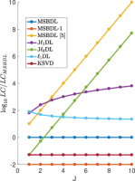
Figure 5: Learning complexity

V Modeling More Complex Relationships

The drawback of the one-to-one prior in (8) is that it constrains $M_{j}=M\;\forall j$. In the following, we propose two models which allow for $M_{j}$ to be modality-dependent. For ease of exposition, we set $J=2$, but the models we describe can be readily expanded to $J>2$. We propose to organize $\bm{x}$ into a tree with $K$ disjoint branches. We adopt the convention that the elements of $x_{1}$ and $x_{2}$ form the roots and leaves of the tree, respectively. The root of the $k$’th branch is $x_{1}[k]$ and the leaves are indexed by $\mathscr{T}^{k}\subseteq[M_{2}]$. The defining property of the models we propose is the relationship between the sparsity pattern of the root and leaf levels.

V-A Atom-to-subspace sparsity

(a)

(b)

Figure 6: Prototype branches for the atom-to-subspace (6(a)) and hierarchical sparsity (6(b)) models.

The one-to-one prior in (8) can be viewed as linking the one-dimensional subspaces spanned by $d_{1}^{m}$ and $d_{2}^{m}$ for $m\in[M]$. Whenever $d_{1}^{m}$ is used to represent $y_{1}$, $d_{2}^{m}$ is used to represent $y_{2}$, and vice-versa. The extension to the multi-dimensional subspace case stipulates that if $d_{1}^{k}$ is used to represent $y_{1}$, then $\left\{d_{2}^{m}\right\}_{m\in\mathscr{T}^{k}}$ is used to represent $y_{2}$, and vice-versa. This model does not constrain $|\mathscr{T}^{k}|$ to be the same for all $k$, such that $M_{2}$ can be chosen independently of $M_{1}$.

Let ${\gamma_{B}}\in\mathbb{R}_{+}^{K}$, in contrast to Section II where $\gamma\in\mathbb{R}_{+}^{M}$. We encode the atom-to-subspace sparsity prior by assigning a single hyperparameter $\gamma_{B}[k]$ to each branch $k$. The distribution $p\left(\bm{x}|\gamma_{B}\right)$ is then given by

$$\prod_{k\in[K]}\mathsf{N}\left(x_{1}[k];0,\gamma_{B}[k]\right)\prod_{m\in\mathscr{T}^{k}}\mathsf{N}\left(x_{2}[m];0,\gamma_{B}[k]\right).$$ (23)

Fig. 6(a) shows a prototype branch under the atom-to-subspace prior. Inference for the prior in (23) proceeds in much the same way as in Section II-A. The form of the marginal likelihood in (10) and posterior in (12) remain the same, with the exception that $\Sigma_{y,j}^{i}$ and $\Sigma_{x,j}^{i}$ are re-defined to be

$$\Sigma_{y,j}^{i} =\sigma_{j}^{2}\mathsf{I}+D_{j}\Gamma_{j}^{i}D_{j}^{T}$$ (24)

$$\Sigma_{x,j}^{i} =\left({\sigma_{j}^{-2}D_{j}^{T}D_{j}+\left({\Gamma_{j}^{i}}\right)^{-1}}\right)^{-1},\Gamma_{1}^{i}=diag(\gamma_{B}^{i}),$$

where $\Gamma_{2}^{i}$ is a diagonal matrix whose $[m,m]$’th entry is $\gamma^{i}_{B}[k]$ for $m\in\mathscr{T}^{k}$. The update of $\gamma_{B}^{i}$ is given by

$$\frac{\Sigma_{x,1}^{i}[m,m]+\left(\mu_{1}^{i}[m]\right)^{2}+\sum_{m\in\mathscr{T}^{k}}\Sigma_{x,2}^{i}[m,m]+\left(\mu_{2}^{i}[m]\right)^{2}}{1+|\mathscr{T}^{k}|},$$

while the update of $D_{j}$ remains identical to (16). There are many ways to extend the atom-to-subspace prior for $J>2$, depending on the specific application. One possibility is to simply append more branches to the root at $x_{1}[k]$ corresponding to coefficients from modalities $j>2$.

One problem is that, for $|\mathscr{T}^{k}|>1$, the atoms of $D_{2}$ indexed by $\mathscr{T}^{k}$ are not identifiable. The reason for the identifiability issue is that $D_{2}$ appears in the objective function in (10) only through the $D_{2}\Gamma_{2}D_{2}^{T}$ term in (24), which can be written as

$$D_{2}\Gamma_{2}D_{2}^{T}=\sum_{k\in[K]}\gamma_{B}[k]\sum_{m\in\mathscr{T}^{k}}d_{2}^{m}\left(d_{2}^{m}\right)^{T}.$$ (25)

Therefore, any $D_{2}^{{}^{\prime}}$ which satisfies $\sum_{m\in\mathscr{T}^{k}}{d^{\prime}}_{2}^{m}\left({d^{\prime}}_{2}^{m}\right)^{T}=\sum_{m\in\mathscr{T}^{k}}d_{2}^{m}\left(d_{2}^{m}\right)^{T}$ for all $k$ achieves the same objective function value as $D_{2}$. Since the objective function is agnostic to the individual atoms of $D_{2}$, the performance of this model is severely upper-bounded in terms of the ability to recover $D_{2}$. In the following, we propose an alternative model which circumvents the identifiability problem.

V-B Hierarchical Sparsity

In this section, we propose a model which allows the root of each branch to control the sparsity of the leaves, but not vice-versa. Specifically, we stipulate that if $x_{1}[k]=0$, then $x_{2}[m]=0\;\forall m\in\mathscr{T}^{k}$. Hierarchical sparsity was first studied in [44, 45, 46] and later incorporated into a unimodal dictionary learning framework in [47]. Later, Bayesian hierarchical sparse signal recovery techniques were developed, which form the basis for the following derivation [48, 49].

From an optimization point of view, hierarchical sparsity can be promoted through a composite regularizer [46]. In this case, the regularizer could take the form

$$\sum_{k\in[K],m\in\mathscr{T}^{k}}\left\|\begin{bmatrix}x_{1}[k]&x_{2}\left[m\right]\end{bmatrix}\right\|_{2}+|x_{2}[m]|.$$ (26)

As described in [46], the key to designing a composite regularizer for a given root-leaf pair is to measure the group norm of the pair along with the energy of the leaf alone. The combination of the group and individual norms serve two purposes which, jointly, promote hierarchical sparsity [46]:

1. It is possible that $x_{2}[m]=0,m\in\mathscr{T}^{k}$, without requiring $x_{1}[k]=0$.

2. The infinitesimal penalty on $x_{1}[k]$ deviating from $0$ tends to $0$ for $|x_{2}[m]|>0,m\in T^{k}$.

The choice of $\ell_{2}$-norm in (26) guarantees that the regularizer satisfies R2 [Theorem 1, [46]]. The conditions of [Theorem 1, [46]] are violated if the $\ell_{2}$ norm is replaced by an $\ell_{1}$ norm in (26).

In a Bayesian setting, we can mimic the effect of the regularizer in (26) through an appropriately defined prior on $\bm{x}$. Let

$$\tilde{x}_{j} =S_{j}x_{j},\;\;S_{1}\in\mathbb{B}^{M_{2}\times M_{1}},\;\;S_{2}=\begin{bmatrix}\mathsf{I}&\mathsf{I}\end{bmatrix}^{T}\in\mathbb{B}^{2M_{2}\times M_{2}}$$ (27)

where $S_{1}$ is a binary matrix such that $S_{1}[m,k]=1$ if and only if $m\in\mathscr{T}^{k}$. Let $R_{j}$ be a diagonal matrix such that $S_{j}^{T}S_{j}R_{j}=\mathsf{I}$ and define $\hat{x}_{j}=S_{j}R_{j}x_{j}$. Let ${\gamma_{j}}\in\mathbb{R}^{M_{2}}\;\forall j$ and

$$p\left(\bm{x}|\bm{\gamma}\right) =\mathsf{N}\left(\hat{x}_{1};0,\Gamma_{1}\right)\mathsf{N}\left(\hat{x}_{2};0,\Gamma_{2}\right),$$ (28)

where $\Gamma_{1}=diag(\gamma_{1})$ and $\Gamma_{2}=diag\left(\begin{bmatrix}\gamma_{1}^{T}&\gamma_{2}^{T}\end{bmatrix}^{T}\right)$. A prototype branch for the hierarchical sparsity prior is shown in Fig. 6(b). To see how this model leads to hierarchical sparsity, observe that

$$\begin{split}p\left(x_{1}[k]|\bm{\gamma}\right)&=\mathsf{N}\left(0,\gamma_{1}[k]\right)\\ p\left(x_{2}[m]|\bm{\gamma}\right)&=\mathsf{N}\left(0,\left({\gamma_{1}^{-1}[k]+\gamma_{2}^{-1}[m]}\right)^{-1}\right)\end{split}$$ (29)

for $m\in\mathscr{T}^{k}$. If we infer that $\gamma_{1}[k]=0$, then the prior on both $x_{1}[k]$ and $x_{2}[m],\forall m\in\mathscr{T}^{k}$, reduces to a dirac-delta function, i.e. if the root is zero, then the leaves must also be zero. On the other hand, if $\gamma_{2}[m]$ is inferred to be $0$, only the prior on $\gamma_{2}[m]$ is affected, i.e. leaf sparsity does not imply root sparsity.

Inference for the tree-structured model proceeds in a similar fashion to that shown in Section II-A, with a few variations. The goal is to optimize (9) through the EM algorithm. The difference here is that we use $\left\{\bm{\hat{X}},\bm{Y},\theta\right\}$ and $\bm{\hat{X}}$ as the complete and nuisance data, respectively. In order to carry out inference, we must first find the posterior density $p\left(\bm{\hat{X}}|\bm{Y},\theta\right)$. It is helpful to first derive the signal model in terms of $\bm{\hat{x}}$ [48]:

$$p\left(y_{j}|D_{j},\hat{x}_{j},\sigma_{j}\right) =\mathsf{N}\left(A_{j}S_{j}^{T}\hat{x}_{j},\sigma_{j}^{2}\mathsf{I}\right).$$ (30)

Using (30), it can be shown that

$$p\left(\hat{x}_{j}^{i}|y_{j}^{i},\theta\right) =\mathsf{N}\left(\mu_{\hat{x},j}^{i},\Sigma_{\hat{x},j}^{i}\right)$$ (31)

$$\Sigma_{\hat{x},j}^{i} =\left({\sigma_{j}^{-2}S_{j}D_{j}^{T}D_{j}S_{j}^{T}+\left({\Gamma_{j}^{i}}\right)^{-1}}\right)^{-1}$$ (32)

$$\mu_{\hat{x},j}^{i} =\sigma_{j}^{-2}\Sigma_{\hat{x},j}^{i}D_{j}S_{j}^{T}y_{j}.$$ (33)

The likelihood function itself is different from (10)-(11) and is given by $p\left(y_{j}^{i}|\theta\right)=\mathsf{N}\left(0,\Sigma_{\hat{y},j}^{i}\right)$, where $\Sigma_{\hat{y},j}^{i}=\sigma_{j}^{2}\mathsf{I}+D_{j}S_{j}^{T}\Gamma_{j}^{i}S_{j}D_{j}^{T}$. The EM update rules are given by

$$\left(\gamma_{j}^{i}[m]\right)^{t+1} =\begin{cases}0.5\sum_{j^{\prime}=1}^{2}\Sigma_{\hat{x},j^{\prime}}^{i}[m,m]+\left(\mu_{\hat{x},j^{\prime}}^{i}[m]\right)^{2}&\text{ if }m\leq M_{2}\\ \Sigma_{\hat{x},j}^{i}[m,m]+\left(\mu_{\hat{x},j}^{i}[m]\right)^{2}&\text{ else. }\end{cases}$$ (34)

$$\left(D_{j}\right)^{t+1} =Y_{j}U_{j}^{T}S_{j}\left({S_{j}^{T}\left(U_{j}U_{j}^{T}+\sum_{i\in[L]}\Sigma_{\hat{x},j}^{i}\right)S_{j}}\right)^{-1}.$$ (35)

Extending the hierarchical sparsity prior for $J>2$ is straightforward and depends on the specific application being considered. It is possible to simply append more leaves to each root $x_{1}[k]$ corresponding to coefficients from modality $j>2$. Another possibility is to treat each $x_{2}[m]$ as itself a root with leaves from $x_{3}$, assigning a hyperparameter to each $x_{2}$-$x_{3}$ root-leaf pair as well as to each $x_{3}$ leaf, and repeating the process until all modalities are incorporated into the tree.

V-C Avoiding Poor Stationary Points

For both the atom-to-subspace and hierarchical sparsity models, we experimentally observe that MSBDL tends to get stuck in undesirable stationary points. In the following, we describe the behavior of MSBDL in these situations and offer a solution. Suppose that data is generated according to the atom-to-subspace model, where $D_{j}$ denotes the true dictionary for modality $j$. In this scenario, we experimentally observe that MSBDL performs well when $|\mathscr{T}^{k}|=c\;\forall k$. On the other hand, if $|\mathscr{T}^{k}|$ varies as a function of $k$, MSBDL tends to get stuck in poor stationary points, where the quality of a stationary point is (loosely) defined next. Let $|\mathscr{T}^{k}|=1$ for all $k$ except $k^{\prime}$, for which $|\mathscr{T}^{k^{\prime}}|=2$, i.e. $M_{2}=M_{1}+1$. In this case, MSBDL is able to recover $D_{1}$, but recovers only the atoms of $D_{2}$ which are indexed by $\mathscr{T}^{k}\;\;\forall k\neq k^{\prime}$.

To avoid poor stationary points, we adopt the following strategy. If the tree describing the assignment of columns of $D_{2}$ to those of $D_{1}$ is unbalanced, i.e. $|\mathscr{T}^{k}|$ varies with $k$, then we first balance the tree by adding additional leaves. Let $\hat{M}_{2}$ be the number of leaves in the balanced tree. We run MSBDL until convergence to generate $\bm{\hat{D}}$. Finally, we prune away $\hat{M}_{2}-M_{2}$ columns of $\hat{D}_{2}$ using the algorithm in Fig. 7.

1:$D,U,\{\mathscr{T}^{k}\}_{k\in[K]},M_{p},S,\epsilon$

2:Let $z[m]=\left\|\left(S^{T}U\right)[m,:]\right\|_{2}^{2}\;\forall m$ and

$$v[k]=\operatorname*{arg\,max}_{m_{1},m_{2}\in\mathscr{T}^{k}\text{ s.t. }m_{1}\neq m_{2}}\frac{|\left(d^{m_{1}}\right)^{T}d^{m_{2}}|}{\|d^{m_{1}}\|_{2}\|d^{m_{2}}\|_{2}}$$

3:while $\exists k\text{ s.t. }v[k]>\epsilon\text{ and }|\mathscr{T}^{k}|>1\text{ and }M_{p}>0$ do

4:     $k=\operatorname*{arg\,max}_{k}v[k]$

5:     Find $m=\operatorname*{arg\,min}_{m\in\mathscr{T}^{k}}z[m]$

6:     Remove column $m$ from $D$ and $\mathscr{T}^{k}$

7:     $M_{p}\leftarrow M_{p}-1$

8:end while

9:while $M_{p}>0$ do

10:     Find $m=\operatorname*{arg\,min}_{m\in\mathscr{T}^{k}\text{ s.t. }|\mathscr{T}^{k}|>1}z[m]$

11:     Remove column $m$ from $D$ and $\mathscr{T}^{k}$

12:     $M_{p}\leftarrow M_{p}-1$

13:end while

Figure 7: Pruning algorithm for the learning strategy in Section V-C. $M_{p}$ denotes the number of columns to be pruned, $S$ is given by the identity matrix for the atom-to-subspace model and by $S_{2}$ in (27) for the hierarchical sparsity model, and $U$ denotes the matrix of first order sufficient statistics.

VI Task Driven MSBDL (TD-MSBDL)

In the following, we describe a task-driven extension of the MSBDL algorithm. For purposes of exposition, we assume the one-to-one prior in (8), but the approach applies equally to the priors discussed in Section V, as discussed in Section VIII. To incorporate task-driven learning, we modify the MSBDL graphical model to the one shown in Fig. 8. We set $p\left(h|x_{j},W_{j}\right)=\mathsf{N}\left(W_{j}x_{j},\beta_{j}^{2}\mathsf{I}\right)$, where $\beta_{j}$ is the class label noise standard deviation for modality $j$. The class label noise standard deviation is modality dependent, affording the model an extra level of flexibility compared to [16, 13, 20]. The choice of the Gaussian distribution for the conditional density of ${h}$, as opposed to a multinomial or softmax, stems from the fact that the posterior $p\left(x_{j}|y_{j},h,{D}_{j},{W}_{j}\right)$ needed to perform EM remains computable in closed form, i.e. $p\left(x_{j}^{i}|y_{j}^{i},h^{i},{D}_{j},{W}_{j}\right)=\mathsf{N}\left({\Sigma}_{x,j}^{TD,i},{\mu}_{j}^{TD,i}\right)$ where

$${\Sigma}_{x,j}^{TD,i} =\left({\sigma_{j}^{-2}{D_{j}^{T}D_{j}}+\beta_{j}^{-2}W_{j}^{T}W_{j}+\left({\Gamma^{i}}\right)^{-1}}\right)^{-1}$$ (36)

$${\mu}_{j}^{TD,i} ={\Sigma}_{x,j}^{TD,i}\left(\sigma_{j}^{-2}{D}_{j}^{T}y_{j}^{i}+\beta_{j}^{-2}{W}_{j}^{T}h^{i}\right)$$ (37)

Figure 8: Graphical model for two modality TD-MSBDL.

VI-A Inference Procedure

We employ EM to optimize

$$\operatorname*{arg\,max}_{\theta^{TD}}\log p\left(\bm{Y},H|\theta^{TD}\right)$$ (38)

where $\theta^{TD}=\left\{\theta,\bm{W}\right\}$. It can be shown that $p\left(y_{j},h|x_{j},\theta^{TD}\right)=\mathsf{N}\left(\begin{bmatrix}y_{j}^{T}&h^{T}\end{bmatrix}^{T};0,\Sigma_{y,j}^{TD}\right)$ where

$$\Sigma_{y,j}^{TD}=\begin{bmatrix}\sigma_{j}^{2}\mathsf{I}+D_{j}\Gamma D_{j}^{T}&0\\ 0&\beta_{j}\mathsf{I}+W_{j}\Gamma W_{j}^{T}\end{bmatrix}.$$ (39)

The update rules for $\bm{D}$ and $\left\{\gamma^{i}\right\}_{i\in[L]}$ remain identical to (15) and (16), respectively, with the exception that the modified posterior statistics shown in (36)-(37) are used. The update of $W_{j}$ is given by

$$W_{j}^{t+1} =H\left({U}_{j}^{TD}\right)^{T}\left({{{U}_{j}^{TD}}\left({U}_{j}^{TD}\right)^{T}+\sum_{i\in[L]}{\Sigma}_{x,j}^{TD,i}}\right)^{-1}$$ (40)

$$U_{j}^{TD} =\begin{bmatrix}\mu_{j}^{TD,1}&\cdots&\mu_{j}^{TD,L}\end{bmatrix}.$$ (41)

We also find it useful to add regularization in the form of $\nu\sum_{j\in[J]}\|W_{j}\|_{F}^{2}$, leading to the update rule

$$W_{j}^{t+1} =\begin{bmatrix}H\left({U}_{j}^{TD}\right)^{T}&0\end{bmatrix}\left({\begin{bmatrix}U_{j}^{TD}\left(U_{j}^{TD}\right)^{T}+\sum_{i\in[L]}\Sigma_{x,j}^{TD,i}&\sqrt{\nu}\mathsf{I}\end{bmatrix}}\right)^{-1}.$$ (42)

TD-MSBDL has the same worst-case computational complexity as MSBDL with the benefit of supervised learning.

VI-B Complete Algorithm

Supervised learning algorithms are ultimately measured by their performance on test data. While a given algorithm may perform well on training data, it may generalize poorly to test data . To maintain the generalization properties of the model, it is common to split the training data into a training set $\left\{\bm{Y},H\right\}$ and validation set $\left\{\bm{Y^{V}},H^{V}\right\}$, where the number of training points $L$ does not necessarily have to equal the number of validation points $L^{V}$. The validation set is then used during the training process as an indicator of generalization, as summarized by the following rule of thumb: Continue optimizing $\theta^{TD}$ until performance on the validation set stops improving. In the context of TD-MSBDL, the concept of generalization has a natural Bayesian definition: The parameter set $\left\{\theta^{TD},\bm{\beta}\right\}$ which achieves optimal generalization solves

$$\operatorname*{arg\,max}_{\theta^{TD}\in\mathscr{H},\bm{\beta}}\prod_{j\in[J]}p\left(H^{V}|\theta^{TD},\beta_{j}\right),$$ (43)

where $\mathscr{H}$ denotes the set of solutions to (38). Note that $p\left(H^{V}|\theta^{TD},\beta_{j}\right)=p\left(H^{V}|W_{j},\beta_{j}\right)$, which is intractable to compute since it requires integrating $p\left(h^{V,i}|W_{j},\gamma^{V,i},\beta\right)=\mathsf{N}\left(0,\beta_{j}\mathsf{I}+W_{j}\Gamma^{V,i}W_{j}^{T}\right)$ over $\gamma^{V,i}$, where $\Gamma^{V,i}=diag(\gamma^{V,i})$. As such, we approximate $p\left(H^{V}|W_{j},\beta_{j}\right)$ by $p\left(H^{V}|W_{j},\gamma^{*,V,i},\beta_{j}\right)$, where $\gamma^{*,V,i}$ is the output of MSBDL with fixed $D_{j}$ for input data $y_{j}^{V,i}$, leading to the tractable optimization problem

$$\operatorname*{arg\,max}_{\theta^{TD}\in\mathscr{H},\bm{\beta}}\prod_{j\in[J]}p\left(H^{V}|W_{j},\left\{\gamma^{*,V,i}\right\}_{i\in[L^{V}]},\beta_{j}\right).$$ (44)

What remains is to select $\bm{\beta}$. As $\beta_{j}$ decreases, TD-MSBDL fits the parameters $\theta^{TD}$ to the training data to a larger degree, i.e. the optimizers of (38) achieve increasing objective function values. Since direct optimization of (44) over $\bm{\beta}$ presents the same challenges as the optimization of $\bm{\sigma}$, we propose an annealing strategy which proposes progressively smaller values of $\beta_{j}$ until the objective in (44) stops improving:

$$\beta_{j}^{t+1}=\begin{cases}\tilde{\beta}_{j}^{t+1}&\text{ if }\log p\left(H^{V}|W_{j},\left\{\gamma^{*,V,i}\right\}_{i\in[L^{V}]},\tilde{\beta}_{j}^{t+1}\right)>\\ &\log p\left(H^{V}|W_{j},\left\{\gamma^{*,V,i}\right\}_{i\in[L^{V}]},{\beta}_{j}^{t}\right)\\ \beta_{j}^{t}&\text{ else }\end{cases}$$ (45)

where $\beta_{j}^{0}>\beta^{\infty}\geq 0,\alpha_{\beta}<1,\tilde{\beta}_{j}^{t+1}=\max(\beta^{\infty},\alpha_{\beta}\beta_{j}^{t})$, and we make the same recommendations for setting $\bm{\beta^{0}}$ and $\beta^{\infty}$ as $\bm{\sigma^{0}}$ and $\sigma^{\infty}$ in Section III. Computing (45) is computationally intensive because it requires running MSBDL, so we only update $\log p\left(H^{V}|W_{j},\left\{\gamma^{*,V,i}\right\}_{i\in[L^{V}]},{\beta}_{j}^{t}\right)$ every $T^{V}$ iterations. Due to space considerations, the complete TD-MSBDL algorithm is provided in the Supplementary Material. Given test data $Y_{j}^{test}$, we first run MSBDL with $D_{j}$ fixed and treat $\mu_{j}^{test,i}$ as an estimate of $x_{j}^{test,i}$. The data is then classified according to $\operatorname*{arg\,max}_{c\in[C]}\left(W_{j}\mu_{j}^{test,i}\right)[c]$, where $e_{c}$ refers to the $c$’th standard basis vector [16].

VII Analysis

We begin by analyzing the convergence properties of MSBDL. Note that MSBDL is essentially a block-coordinate descent algorithm with blocks $\theta$ and $\bm{\sigma}$. Therefore, we first analyze the $\theta$ update block, then the $\bm{\sigma}$ update block, and finally the complete algorithm. Unless otherwise specified, we assume a non-informative prior on $\gamma$ and the one-to-one prior. While MSBDL relies heavily on EM, it is not strictly an EM algorithm because of the $\bm{\sigma}$ annealing procedure. It will be shown that MSBDL still admits a convergence guarantee and an argument will be presented for why annealing $\bm{\sigma}$ produces favorable results in practice. Although we focus specifically on MSBDL, the results can be readily extended to TD-MSBDL, with details omitted for brevity. Proofs for all results are shown in the Supplementary Material.

We first prove that the set of iterates $\left\{\theta^{t}\right\}_{t=1}^{\infty}$ produced by the inner loop of MSBDL converge to the set of stationary points of the log-likelihood with respect to $\theta$. This is established by proving that the objective function is coercive (Theorem 1), which means that $\left\{\theta^{t}\right\}_{t=1}^{\infty}$ admits at least one limit point (Corollary 1), and then proving that limit points are stationary (Theorem 2).

Theorem 1

Let $\left\{\sigma_{j}>0\right\}_{j\in[J]}$, let there be at least one $j^{*}$ for each $m$ such that $\left\|d_{j^{*}}^{m}\right\|_{2}>0$, and let $\exists i$ such that $\gamma^{i}[m]>0$ for any choice of $m$. Then, $-\log p\left(\bm{Y}|\theta,\bm{\sigma}\right)$ is a coercive function of $\left\{\theta,\bm{\sigma}\right\}$.

Corollary 1

Let the conditions of Theorem 1 be satisfied. Then, the sequence $\left\{\theta^{t}\right\}_{t=1}^{\infty}$ produced by the inner loop of the MSBDL algorithm admits at least one limit point.

The proof of Corollary 1 is shown in the Appendix, but the high level argument is that $\left\{\theta^{t}\right\}_{t=1}^{\infty}$ is a member of a compact set. As such $\left\{\theta^{t}\right\}_{t=1}^{\infty}$ admits at least one convergent subsequence. Since there may be multiple convergent subsequences, Corollary 1 does not preclude $\left\{\theta^{t}\right\}_{t=1}^{\infty}$ having multiple limit points, or a limit set. The point is that $\left\{\theta^{t}\right\}_{t=1}^{\infty}$ admits one or more limit points, and Theorem 2 below proves each of these points to be stationary.

Theorem 2

Let the conditions of Corollary 1 be satisfied, $D_{j}^{t}$ be full rank for all $t$ and $j$, $\bm{\sigma}$ be fixed, and generate $\{\theta^{t}\}_{t=1}^{\infty}$ using the inner loop of MSBDL. Then, $\{\theta^{t}\}_{t=1}^{\infty}$ converges to the set of stationary points of $\log p\left(\bm{Y}|\theta,\bm{\sigma}\right)$. Moreover, $\left\{\log p\left(\bm{Y}|\theta,\bm{\sigma}\right)\right\}_{t=1}^{\infty}$ converges monotonically to $\log p\left(\bm{Y}|\theta^{*},\bm{\sigma}\right)$, for stationary point $\theta^{*}$.

The requirement that $D_{j}^{t}$ be full rank is easily satisfied in practice as long as $L>N_{j}$. Note that the SBL algorithm in [24] is a special case of MSBDL for fixed $\bm{D}$ and $J=1$. To the best of our knowledge, Theorem 2 represents the first result in the literature guaranteeing the convergence of SBL. A similar result to Theorem 2 can be given in the stochastic EM regime.

Theorem 3

Let $\bm{\sigma}$ be fixed, $U_{j}^{t}$ be full rank for all $t,j$, and generate $\{{\theta}^{t}\}_{t=1}^{\infty}$ using the inner loop of MSBDL, only updating the sufficient statistics for a batch of points at each iteration (i.e. incremental EM). Then, the limit points of $\{{\theta}^{t}\}_{t=1}^{\infty}$ are stationary points of $\log p\left(\bm{Y}|\theta,\bm{\sigma}\right)$.

If we consider the entire MSBDL algorithm, i.e. including the update of $\bm{\sigma}$, we can still show that MSBDL is convergent.

Corollary 2

Let the conditions of Theorems 1 and 2 be satisfied. Then, the sequence $\left\{\theta^{t},\bm{\sigma^{t}}\right\}_{t=1}^{\infty}$ produced by the MSBDL algorithm admits at least one limit point.

Although the preceding results establish that MSBDL has favorable convergence properties, the question still remains as to why we choose to anneal $\sigma_{j}$. At a high level, it can be argued that setting $\sigma_{j}$ to a large value initially and then gradually decreasing it prevents MSBDL from getting stuck in poor stationary points with respect to $\theta$ at the beginning of the learning process. To motivate this intuition, consider the log likelihood function in (9), which decomposes into a sum of $J$ modality-specific log-likelihoods. The curvature of the log-likelihood for modality $j$ depends directly on $\sigma_{j}$. Setting a high $\sigma_{j}$ corresponds to choosing a relatively flat log likelihood surface, which, from an intuitive point of view, has less stationary points. This intuition can be formalized in the scenario where $D_{j}$ is constrained in a special way.

Theorem 4

Let $\sigma_{j}^{1}>\sigma_{j}^{2},\Psi_{j}=\{D_{j}:D_{j}=\begin{bmatrix}\check{D}_{j}&\mathsf{I}\end{bmatrix}\}$, and $\Omega_{\sigma_{j},j}=\left\{\Sigma_{y,j}:\Sigma_{y,j}=\sigma_{j}^{2}\mathsf{I}+D_{j}\Gamma{D_{j}}^{T},D_{j}\in\Psi_{j}\right\}$. Then, $\Omega_{\sigma_{j}^{1},j}\subseteq\Omega_{\sigma_{j}^{2},j}$.

Theorem 4 suggests that as $\sigma_{j}$ gets smaller, the space over which the log-likelihood in (9) is optimized grows. As the optimization space grows, the number of stationary points grows as well. As a result, it may be advantageous to slowly anneal $\sigma_{j}$ in order to allow MSBDL to learn $D_{j}$ without getting stuck in a poor stationary point.

If we constrain the space over which $D_{j}$ is optimized to $\Psi_{j}$, as in Theorem 4, then we can establish a number of interesting convergence results.

Theorem 5

Let $\alpha_{\sigma}$ be arbitrarily close to $1$, $\sigma^{\infty}=0$, $\sigma_{j}^{0}\geq\operatorname*{arg\,max}_{\sigma_{j}}\max_{\theta}\log p\left(Y_{j}|\theta,\sigma_{j}\right)$, $D_{j}\in\Psi_{j}$, $\theta^{t}=\operatorname*{arg\,max}_{\theta}\log p\left(Y_{j}|\theta,\sigma_{j}^{t-1}\right)$, and consider updating $\sigma_{j}$ using (20). Then, $\sigma_{j}^{t}=\sigma_{j}^{t-1}$ implies $\sigma_{j}^{t}=\operatorname*{arg\,max}_{\sigma_{j}}\log p\left(Y_{j}|\theta^{t},\sigma_{j}\right)$.

Theorem 5 states that, under certain conditions, annealing terminates for a given modality $j$ at a global maximum of the log-likelihood with respect to $\sigma_{j}$ for fixed $\theta^{t}$. The conditions of Theorem 5 ensure that (20) only terminates at stationary points of the log-likelihood.

Theorem 6

Let the conditions of Theorems 2 and 5 and Corollary 2 be satisfied. Then, the sequence $\left\{{\theta}^{t},\bm{\sigma^{t}}\right\}_{t=1}^{\infty}$ produced by MSBDL converges to the set of stationary points of $\log p\left(\bm{Y}|\theta,\bm{\sigma}\right)$.

Convergence results like Theorem 6 cannot be established for K-SVD and J$\ell_{0}$DL because they rely on greedy search techniques. In addition, no convergence results are presented in [16] for J$\ell_{1}$DL.

Finally, we consider what guarantees can be given for dictionary recovery in the noiseless setting, i.e. $Y_{j}=D_{j}X_{j}\;\;\forall j.$ We assume $M_{j}=M\;\forall j$ and that $\bm{x^{i}}$ share a common sparsity profile for all $i$. We do not claim that the following result applies to more general cases when $M_{j}\neq M\;\forall j$ or different priors. The question we seek to answer is: Under what conditions is the factorization $Y_{j}=D_{j}X_{j}$ unique? Due to the nature of dictionary learning, uniqueness can only be considered up to permutation and scale. Two dictionaries $D^{1}$ and $D^{2}$ are considered equivalent if $D^{1}=D^{2}Z$, where $Z$ is a permutation and scaling matrix. Guarantees of uniqueness in the unimodal setting were first studied in [50]. The results relied on several assumptions about the data generation process.

Assumption 1

Let $s=\|x_{j}^{i}\|_{0}\;\forall i,j$, and $s<\frac{\text{spark}(D_{j})}{2}$, where $\text{spark}(D_{j})$ is the minimum number of columns of $D_{j}$ which are linearly dependent [51]. Each $x_{j}^{i}$ has exactly $s$ non-zeros.

Assumption 2

$Y_{j}$ contains at least $s+1$ different points generated from every combination of $s$ atoms of $D_{j}$.

Assumption 3

The rank of every group of $s+1$ points generated by the same $s$ atoms of $D_{j}$ is exactly $s$. The rank of every group of $s+1$ points generated by different atoms of $D_{j}$ is exactly $s+1$.

Lemma 1 (Theorem 3, [50])

Let Assumptions 1-3 be true. Then, $Y_{j}$ admits a unique factorization $D_{j}X_{j}$. The minimum number of samples required to guarantee uniqueness is given by $(s+1)\binom{M}{s}$.

Treating the multimodal dictionary learning problem as $J$ independent unimodal dictionary learning problems, the following result follows from Lemma 1.

Corollary 3

Let Assumptions 1-3 be true for all $j$. Then, $Y_{j}$ admits a unique factorization $D_{j}X_{j}$ for all $j$. The minimum number of samples required to guarantee uniqueness is given by $J(s+1)\binom{M}{s}$.

As the experiments in Section VIII will show, there are benefits to jointly learning multimodal dictionaries. It is therefore interesting to inquire whether or not there are provable benefits to the multimodal dictionary learning problem, at least from the perspective of the uniqueness of factorizations. To formalize this intuition, consider the scenario where some data points $i$ do not have data available for all modalities. Let the Boolean matrix $P\in\mathbb{B}^{J\times L}$ be defined such that $P[j,i]$ is $1$ if data for modality $j$ is available for instance $i$ and $0$ else. The conditions on the amount of data needed to guarantee unique recovery of $\bm{D}$ by Corollary 3 can be restated as $L=(s+1)\binom{M}{s}$ and $P[j,i]=1\;\forall j,i$. The natural question to ask next is: Can uniqueness of factorization be guaranteed if $P[j,i]=0$ for some $(j,i)$?

Theorem 7

Let $\bm{x^{i}}$ share a common sparsity profile for all $i$ and Assumptions 1-2 be true for all $j$. Let Assumption 3 be true for a single $j^{*}$. Let $G_{j}^{k}=\left\{i:P[j,i]=1\text{ and }y_{j}^{i}\in\text{span}\left(D_{j}[:,\Upsilon^{k}]\right)\right\}$ where $\Upsilon^{k}$ is the $k$’th subset of size $s$ of $[M]$. Let $|G_{j}^{k}\cap G_{j^{*}}^{k}|\geq s$ for all $j\neq j^{*}$ and $k$. Then, the factorization $Y_{j}=D_{j}X_{j}$ is unique for all $j$. The minimum total number of data points required to guarantee uniqueness is given by $J\left(s+\frac{1}{J}\right)\binom{M}{s}$.

Theorem 7 establishes that the number of samples required to guarantee a unique solution to the multimodal dictionary learning problem is strictly less than in Corollary 3.

VIII Results

VIII-A Synthetic Data Dictionary Learning

To validate how well MSBDL is able to learn unimodal and multimodal dictionaries, we conducted a series of experiments on synthetic data. We adopt the setup from [52] and generate ground-truth dictionaries $D_{j}\in\mathbb{R}^{20\times 50}$ by sampling each element from a $\mathsf{N}(0,1)$ distribution and scaling the resulting matrices to have unit $\ell_{2}$ column norm. We then generate $x_{j}^{i}$ by randomly selecting $s=5$ indices and generating the non-zero entries by drawing samples from a $\mathsf{N}(0,1)$ distribution. The supports of $\bm{x^{i}}$ are constrained to be the same, while the coefficients are not. The elements of $v_{j}^{i}$ are generated by drawing samples from a $\mathsf{N}(0,1)$ distribution and scaling the resulting vector in order to achieve a specified Signal-to-Noise Ratio (SNR). We use $L=1000$ and simulate both bimodal and trimodal datasets. The bimodal dataset consists of $30$dB ($j=1$) and $10$dB ($j=2$) SNR modalities. The trimodal dataset consists of $30$ dB ($j=1$), $20$ dB ($j=2$), and $10$ dB ($j=3$) SNR modalities. We use the empirical probability of recovering $\bm{D}$ as the measure of success, which is given by

$$\frac{1}{M_{j}}\sum_{m\in[M_{j}]}\mathbbm{1}\left[\iota\left(d_{j}^{m},\hat{D}_{j}\right)>0.99\right]$$ (46)

$$\iota\left(d_{j}^{m},\hat{D}_{j}\right)=\max_{1\leq m^{\prime}\leq M_{j}}\frac{\left|\left(d_{j}^{m}\right)^{T}\hat{d}_{j}^{m^{\prime}}\right|}{\left\|d_{j}^{m}\right\|_{2}\left\|d_{j}^{m^{\prime}}\right\|_{2}},$$ (47)

where $\hat{D}_{j}$ denotes the output of the dictionary learning algorithm and $\mathbbm{1}\left[\cdot\right]$ denotes the indicator function. The experiment is performed $50$ times and averaged results are reported. We compare MSBDL with $\ell_{1}$DL, K-SVD, J$\ell_{0}$DL, and J$\ell_{1}$DL. While code for J$\ell_{1}$DL was publicly available, it could not be run on any of our Windows or Linux machines, so we used our own implementation. Code for J$\ell_{0}$DL was not publicly available, so we used our own implementation. For all algorithms, the batch size was set to $L$.

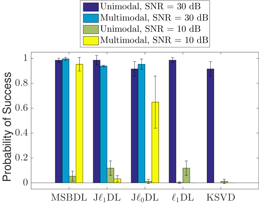
(a)

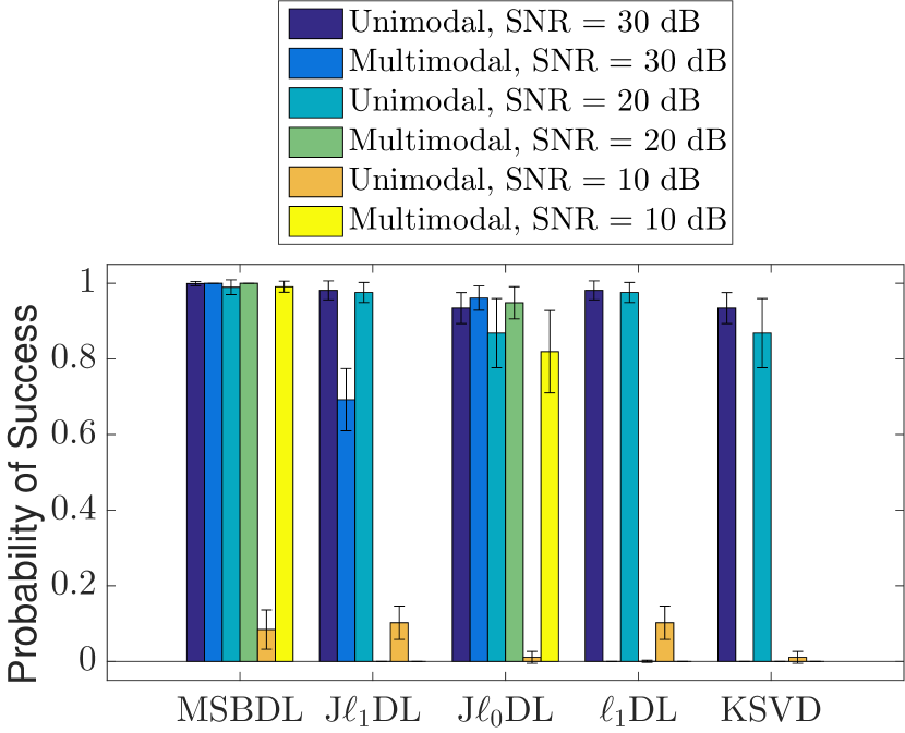
(b)

Figure 9: Bimodal (9(a)) and trimodal (9(b)) synthetic data results with one standard deviation error bars.

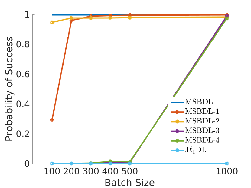
(a)

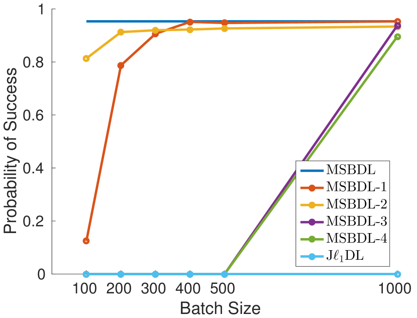
(b)

Figure 10: Bimodal synthetic data results using stochastic learning for $30$ dB (Fig. 10(a)) and $10$ dB (Fig. 10(b)) datasets.

For the bimodal setting, the parameters $\sigma_{1}^{0}$ and $\sigma_{2}^{0}$ were set to $1$ and $\sqrt{10}$, respectively. For the trimodal setting, the parameters $\sigma_{1}^{0},\sigma_{2}^{0},$ and $\sigma_{3}^{0}$ were set to $1,\sqrt{1.5},$ and $\sqrt{2}$, respectively. In both cases, we set $\alpha_{\sigma}=\sqrt{0.995}$ and $\sigma^{\infty}=\sqrt{1e-3}$, where this choice of $\sigma^{\infty}$ corresponds to the lowest candidate $\lambda$ in the cross-validation procedure for competing algorithms. It was experimentally determined that MSBDL is relatively insensitive to the choice of $\sigma_{j}^{0}$ as long as $\sigma_{1}^{0}<\sigma_{2}^{0}<\sigma_{3}^{0}$, thus obviating the need to cross-validate these parameters. The regularization parameters ${\lambda}$ in (1) and $\bm{\lambda}$ in (3) were selected by a grid search over $\{1e-3,1e-2,1e-1,1\}$ and both K-SVD and J0DL were given the true $s$. The parameter $\lambda_{1}$ was set to $1$ for J$\ell_{0}$DL across all experiments because the objective function in (3) depends only on the relative weighting of modalities. All algorithms were run until convergence.

The bimodal and trimodal dictionary recovery results are shown in Fig.’s 9(a) and 9(b), respectively. For unimodal data, all of the algorithms recover the true dictionary almost perfectly when the $\text{SNR }=30\text{ dB}$, with the exception of J0DL and K-SVD. All of the tested algorithms perform relatively well for data with $20$ dB SNR and poorly on data with $10$ dB SNR, although MSBDL outperforms the other tested method in these scenarios. In the multimodal scenario, the proposed method clearly distinguishes itself from the other methods tested. For trimodal data, not only does MSBDL achieve $100\%$ accuracy on the $30$ dB data dictionary, but it achieves accuracies of $100\%$ and $99.2\%$ on the $20$ dB and $10$ dB data dictionaries, respectively. MSBDL outperforms the next best method by $17.2\%$ on the $10$ dB data recovery task. J$\ell_{0}$DL was able to capture some of the multimodal information in learning the $10$ dB data dictionary, but the $10$ dB data dictionary accuracy only reaches $81.9\%$. J$\ell_{1}$DL performs even worse in recovering the $10$ dB data dictionary, achieving $0\%$ accuracy. Similar trends can be seen in the bimodal results.

Next, we evaluate the performance of the MSBDL algorithms in Table III. We repeat the bimodal experiment and compare the proposed methods with J$\ell_{1}$DL, which is the only competing multimodal dictionary learning algorithm that has a stochastic version. The dictionary recovery results are shown in Fig. 10. The results show that J$\ell_{1}$DL is not able to recover any part of either the $30$ dB nor $10$ dB dataset dictionaries. In terms of the asymptotic performance as the batch size approaches $L$, MSBDL-1 exhibits negligible bias on both datasets, whereas the other MSBDL flavors incur a small bias, especially on the $10$ dB dataset. On the other hand, it is interesting that MSBDL-2 dramatically outperforms MSBDL-1 for batch sizes less than $300$, which is unexpected since MSBDL-2 performs approximate sufficient statistic computations. The poor performance of MSBDL-3 and MSBDL-4 suggests that these algorithms should be considered only in extremely memory constrained scenarios. Finally, we report on the performance of the proposed annealing strategy for $\sigma_{j}$. For the bimodal dataset, one expects to $\sigma_{1}$ to converge to a smaller value than $\sigma_{2}$. Fig. 13 shows a histogram of the values to which $\bm{\sigma}$ converge to. The results align with expectations and lend experimental validation for the annealing strategy. We observe the same trend for MSBDL-1 with $L_{0}<L$.

To validate the performance of MSBDL using the atom-to-subspace model, we run a number of synthetic data experiments. In all cases, we use $J=2$ and $L=1000$. We use MSBDL-1 with $L_{0}=500$ to highlight that the algorithm works in incremental EM mode. We simulate $4$ scenarios, summarized in Table V. For each scenario, we first generate the elements of the ground-truth dictionary $\bm{D}$ by sampling from a $\mathsf{N}\left(0,1\right)$ distribution and normalizing the resulting dictionaries to have unit $\ell_{2}$ column norm. We then set $\mathscr{T}^{k}=\{k,k+M_{1}\}\text{ if }k+M_{1}\leq M_{2}$ and $k\text{ otherwise}$. This choice of $\left\{\mathscr{T}^{k}\right\}_{k\in[K]}$ represents the most uniform assignment of columns of $D_{2}$ to columns of $D_{1}$. We then generate $x_{1}^{i}$ by randomly selecting $s=5$ indices and generating the non-zero entries by drawing samples from a $\mathsf{N}(0,1)$ distribution. We use $\left\{\mathscr{T}^{k}\right\}_{k\in[K]}$ to find the support of $x_{2}^{i}$ and generate the non-zero entries by drawing from a $\mathsf{N}(0,1)$ distribution. In order to assess the performance of the learning algorithm, we must first define the concept of distance between multi-dimensional subspaces. We follow [53] and compute the distance between $D_{2}[:,\mathscr{T}^{k}]$ and $\hat{D}_{2}$ using

$$\iota\left(D_{2}[:,\mathscr{T}^{k}],\hat{D}_{2}\right)=\max_{1\leq k^{\prime}\leq K}\sqrt{|V_{1}^{T}V_{2}V_{2}^{T}V_{1}|},$$

where we use $D_{2}[:,\mathscr{T}^{k}]$ to denote the columns of $D_{2}$ indexed by $\mathscr{T}^{k}$, and $V_{1},V_{2}$ denote orthonormal bases for $D_{2}[:,\mathscr{T}^{k}]$ and $\hat{D}_{2}[:,\mathscr{T}^{k^{\prime}}]$, respectively. We then define the distance between $D_{2}$ and $\hat{D}_{2}$ using the two quantities

$$\vartheta_{1}\left(D_{2},\hat{D}_{2}\right) =c_{1}\sum_{k\in\{k:|\mathscr{T}^{k}|=1\}}\mathbbm{1}\left[\iota\left(D_{2}[:,\mathscr{T}^{k}],\hat{D}_{2}\right)>0.99\right]$$

$$\vartheta_{2}\left(D_{2},\hat{D}_{2}\right) =c_{2}\sum_{k\in\{k:|\mathscr{T}^{k}|>1\}}\mathbbm{1}\left[\iota\left(D_{2}[:,\mathscr{T}^{k}],\hat{D}_{2}\right)>0.99\right]$$

where $c_{1}=|\{k:|\mathscr{T}^{k}|=1\}|^{-1}$ and $c_{2}=|\{k:|\mathscr{T}^{k}|>1\}|^{-1}$. We use MSBDL-1 to learn $\bm{\hat{D}}$, with accuracy results reported in Table V. Histograms of results are provided in the Supplementary Materials for a higher resolution perspective into the performance of the proposed approach. Note that Table V reports the accuracy of MSBDL-1 in recovering both the atoms and subspaces of $D_{2}$. Test case A simulates the scenario where both modalities have a high SNR and $M_{2}=2M_{1}$. In other words, test case A tests if MSBDL-1 is able to learn in the atom-to-subspace model, without the complications that arise from added noise. The results show that MSBDL-1 effectively learns both the atoms of $D_{1}$ and the subspaces comprising $D_{2}$. Test case B simulates the scenario where $|\mathscr{T}^{k}|=1$ for some $k$ but not for others. In effect, test case B tests the pruning strategy described in Section V-C and summarized in Fig. 7. The results show that the pruning strategy is effective and allows MSBDL-1 to learn both the atoms of $D_{1}$ and the atoms and subspaces comprising $D_{2}$. Test case C is identical to test case B, but with noise added to modality $2$. The results show that MSBDL-1 still effectively recovers $D_{1}$, but there is a drop in performance with respect to recovering the atoms of $D_{2}$ and a significant drop in recovering the subspaces of $D_{2}$. The histogram in Fig. 11(a) shows that the distribution of $\left\{\iota(D_{2}[:\mathscr{T}^{k}],\hat{D}_{2})\right\}_{k\in K}$ is concentrated near $1$ for test case C, suggesting that an alignment threshold of $0.99$ is simply too strict in this case. Finally, test case D demonstrates that MSBDL-1 exhibits robust performance when the modality comprising the roots of the tree is noisy. To provide experimental evidence for the fact that the atom-to-subspace model is agnostic to the atoms of $D_{2}$, as discussed in Section V-A, we show the ability of MSBDL-1 to recover the atoms of $D_{2}$ for test case $A$ in Fig. 13. The results show that MSBDL-1 is not able to recover the atoms of $D_{2}$.

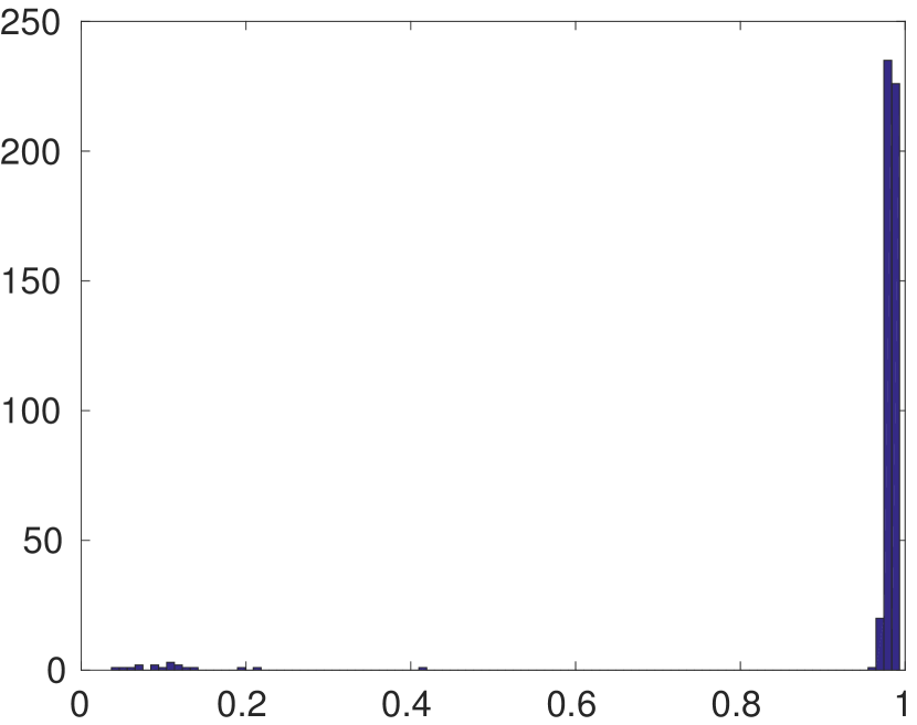
(a)

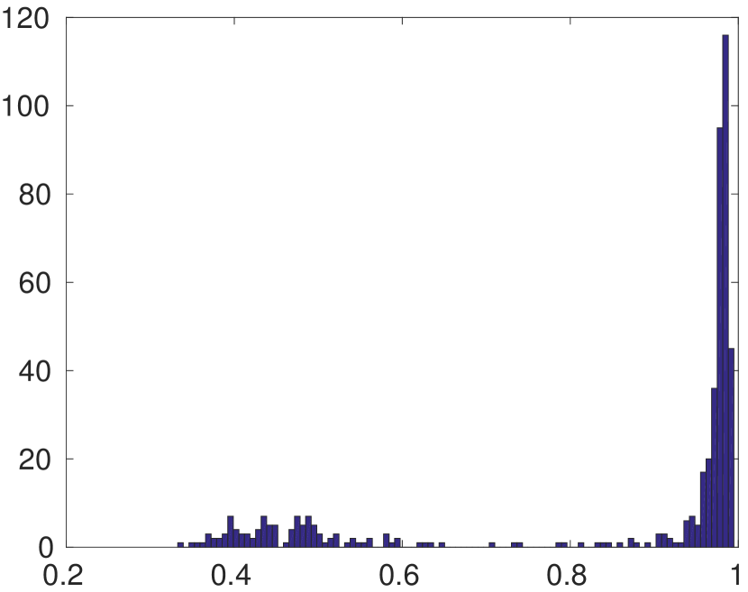
(b)

Figure 11: Histograms of $\iota\left(D_{2}[:,\mathscr{T}^{k}],\hat{D}_{2}\right)$ for test case C in Table V (11(a)) and $\iota\left(D_{2}[:,m],\hat{D}_{2}\right)$ for test case C in Table VI (11(b)).

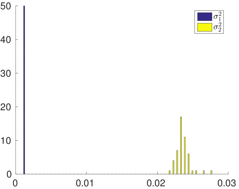
Figure 12: Histogram of $\sigma_{j}^{2}$ at convergence for a bimodal dataset consisting of $30$ dB and $10$ dB modalities.

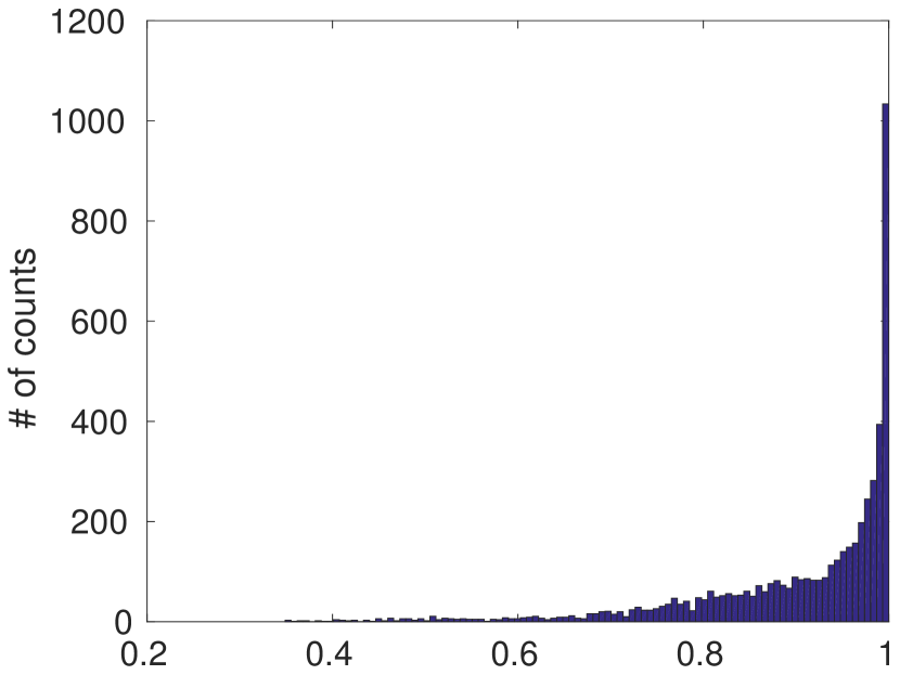
Figure 13: Histogram of $\iota\left(D_{2}[:,m],\hat{D}_{2}\right)\;\forall m$ for test case $A$.

Next, we present experimental results for dictionary learning under the hierarchical model, using the same setup as for the atom-to-subspace model. We simulate $4$ scenarios, summarized in Table VI. To evaluate the performance of the proposed approach, we measure how well it is able to recover the atoms of $D_{1}$ and $D_{2}$, where we distinguish between the atoms of $D_{2}$ corresponding to $|\mathscr{T}^{k}|=1$ and $|\mathscr{T}^{k}|>1$ using

$$\varrho_{1}\left(D_{2},\hat{D}_{2}\right) =c_{3}\sum_{k\in\{k:|\mathscr{T}^{k}|=1\}}\mathbbm{1}\left[\iota\left(D_{2}[:,\mathscr{T}^{k}],\hat{D}_{2}\right)>0.99\right]$$

$$\varrho_{2}\left(D_{2},\hat{D}_{2}\right) =c_{4}\sum_{k\in\{k:|\mathscr{T}^{k}|=1\},m\in\mathscr{T}^{k}}\mathbbm{1}\left[\iota\left(D_{2}[:,m],\hat{D}_{2}\right)>0.99\right]$$

where $c_{3}=|\{k:|\mathscr{T}^{k}|=1\}|^{-1}$ and $c_{4}=|\{k:|\mathscr{T}^{k}|>1\}|^{-1}$. The recovery results are reported in Table VI. Histograms of the results are provided in the Supplementary Material. Test case A demonstrates that MSBDL-1 is able to learn the atoms of $D_{1}$ and $D_{2}$ in the low noise scenario for $M_{2}=2M_{1}$. Test case B shows that MSBDL-1 is able to learn the atoms of $D_{1}$ and $D_{2}$ for $M_{1}<M_{2}<2M_{1}$, i.e. highlighting that the pruning strategy in Fig. 7 is effective for the hierarchical sparsity model. Test case C adds a considerable amount of noise to the modality occupying the leaves of the tree. Although the recovery results in Table VI suggest that MSBDL-1 does not perform well in recovering $D_{2}$ in this scenario, the histogram in Fig. 11(b) shows robust performance. Finally, test case D shows the scenario where a large amount of noise is added to the modality occupying the roots of each subtree.

	$d_{1},M_{1}$	$d_{2},M_{2}$	$SNR_{1}$	$SNR_{2}$	$\vartheta_{1}(D_{1},\hat{D}_{1})$	$\vartheta_{1}(D_{2},\hat{D}_{2})$	$\vartheta_{2}(D_{2},\hat{D}_{2})$
A	$20,50$	$40,100$	$30$	$30$	$99.8$	—	$92$
B	$20,50$	$30,60$	$30$	$30$	$99.5$	$100$	$97$
C	$20,50$	$30,60$	$30$	$10$	$99.9$	$68.05$	$3.6$
D	$20,50$	$30,60$	$10$	$30$	$73.64$	$97.7$	$75.4$

TABLE V: Recovery results using atom-to-subspace model.

	$d_{1},M_{1}$	$d_{2},M_{2}$	$SNR_{1}$	$SNR_{2}$	$\varrho_{1}\left(D_{1},\hat{D}_{1}\right)$	$\varrho_{1}\left(D_{2},\hat{D}_{2}\right)$	$\varrho_{2}\left(D_{2},\hat{D}_{2}\right)$
A	$20,50$	$40,100$	$30$	$30$	$99.3$	—	$96.6$
B	$20,50$	$30,60$	$30$	$30$	$100$	$94.7$	$82.7$
C	$20,50$	$30,60$	$30$	$10$	$100$	$22.1$	$3.3$
D	$20,50$	$30,60$	$10$	$30$	$5.2$	$93.1$	$61.1$

TABLE VI: Recovery results using hierarchical model.

VIII-B Photo Tweet Dataset Classification

We validate the performance of TD-MSBDL on the Photo Tweet dataset [54]. The Photo Tweet dataset consists of 603 tweets covering 21 topics. Each tweet contains text and an image with an associated binary label indicating its sentiment. The dataset consists of 5 partitions. We use these partitions to perform 5 rounds of leave-one-out cross-validation, where, during each round, we use one partition as the test set, one as the validation set, and the remaining partitions as the training set. For each round, we process the images by first extracting a bag of SURF features [55] from the training set using the MATLAB computer vision system toolbox. We then encode the training, validation, and test sets using the learned bag of features, yielding a 500-dimensional representation for each image [56]. Finally, we compute the mean of each dimension across the training set, center the training, validation, and test sets using the computed means, and perform 10 component PCA to generate a 10-dimensional image representation. We process the text data by first building a 2688 dimensional bag of words from the training set using the scikit-learn Python library. We then encode the training, validation, and test sets using the learned bag of words, normalizing the resulting representations by the number of words in the tweet. We then center the data and perform 10 component PCA to yield a 10-dimensional text representation.

We run TD-MSBDL using incremental EM and approximate posterior sufficient statistic computations, referring to the resulting algorithm as TD-MSBDL-2 in accordance with the taxonomy in Table III. Our convention is to refer to the text and image data as modalities $1$ and $2$ respectively. We use $M_{j}=40\forall j$, $L_{0}=200$, $\sigma_{1}^{0}=\sqrt{0.01}$, $\sigma_{2}^{0}=\sqrt{0.2}$, $\beta_{j}^{0}=\sqrt{100}\forall j$, $\sigma^{\infty}=\sqrt{1e-4},\alpha_{\sigma}=\sqrt{0.995}$, $\beta^{\infty}=\sqrt{1e-2},\alpha_{\beta}=\sqrt{0.995}$, and $T^{V}=500$. We compare TD-MSBDL with several unimodal and multimodal approaches. We use TD-$\ell_{1}$DL and D-KSVD to learn classifiers for images and text using unimodal data. For TD-$\ell_{1}$DL we use the validation set to optimize for $\lambda$ over the set $\{1e-3,1e-2,1e-1,1\}$. We also compare with TD-J$\ell_{1}$DL trained on the multimodal data, using the the same validation approach as for TD-$\ell_{1}$DL. In all cases, we run training for a maximum of $15e3$ iterations.

The classification results are shown in Table VII. Comparing TD-MSBDL with the unimodal methods (i.e. TD-$\ell_{1}$DL and D-KSVD), the results show that TD-MSBDL achieves higher performance for both feature types. Moreover, it is interesting that TD-J$\ell_{1}$DL performs worse than TD-$\ell_{1}$DL, suggesting that it is not capable of capturing the multimodal relationships which TD-MSBDL benefits from.

Feature Type	TD-MSBDL-2	TD-J$\ell_{1}$DL	TD-$\ell_{1}$DL	D-KSVD
Images	65.6	59.2	61.1	63.9
Text	76	73.7	74.1	69.4

TABLE VII: Photo tweet dataset classification accuracy $(\%)$.

	TD-MSBDL-2	TD-MSBDL-1	TD-MSBDL-1
Prior	One-to-one (8)	Hierarchical (28)	Atom-to-subspace (23)
$d_{1}\times M_{1}/d_{2}\times M_{2}$	$10\times 40/10\times 40$	$10\times 40/20\times 80$	$10\times 40/20\times 80$
Images	65.6	69.2	69.5
Text	76	74.6	74.3

TABLE VIII: Photo tweet dataset classification accuracy $(\%)$ using TD learning and priors from Section V. Our convention is to designate text as modality 1 and images as modality 2.

Finally, we show the efficacy of the priors in Section V in classifying the Photo Tweet dataset. The goal is to show that, by allowing the number of atoms of the image and text dictionaries to be different, the atom-to-subspace and hierarchical sparsity priors lead to superior classification performance. We begin by extracting features from the text and image data as before, with the exception that we use $20$ PCA components to represent images. We then set $M_{1}$, the text data dictionary size, to $40$ and $M_{2}$, the image dictionary size, to $80$, corresponding to an oversampling factor $M_{j}/N_{j}$ of $4$ for both modalities. We run the TD-MSBDL algorithm with the atom-to-subspace and hierarchical sparsity priors. For the atom-to-subspace prior, the only required modification is to change the update rule of $\gamma^{i}$ to (15). For the hierarchical sparsity prior, the $\gamma^{i}$, $D_{j}$, and $W_{j}$ update rules are modified to (34), (35), and $\left(W_{j}\right)^{t+1}=H\left(U_{j}^{TD}\right)^{T}S_{j}\left({S_{j}^{T}\left(U_{j}^{TD}\left(U_{j}^{TD}\right)^{T}+\sum_{i\in[L]}\Sigma_{\hat{x},j}^{TD,i}\right)S_{j}}\right)^{-1}$, respectively. Because there are significant dependencies among the elements in $x_{j}$ a-priori, we use exact sufficient statistic computation, referring to the resulting algorithm as TD-MSBDL-1. The classification results are presented in Table VIII, where the TD-MSBDL-2 results with one-to-one prior from Section VIII-B are shown for reference. The results show a significant improvement in image classification. Although text classification deteriorates slightly, the text classification rate for both atom-to-subspace and hierarchical priors is still higher than the competing methods in Table VII. Note that this type of experiment, where a different number of dictionary atoms is used for the image and text modalities, is not possible for any of the other dictionary learning approaches considered in this work.

VIII-C CIFAR10

The CIFAR10 dataset consists of $32\times 32$ images from 10 classes [57]. In this experiment, we extract $7\times 7$ patches from images in the dataset to form $Y_{1}$. We then form $Y_{2}$ by adding noise to $Y_{1}$, i.e. $y_{2}=y_{1}+\xi,\xi\sim\mathsf{N}\left(0,\sigma_{\xi}^{2}\mathsf{I}\right)$. Our goal is to learn representations $\left\{D_{j}\right\}_{j\in[J]}$ for $\left\{Y_{j}\right\}_{j\in[J]}$, where $J=2$, and to evaluate the quality of those representations. Since ground truth dictionaries do not exist in this scenario, we evaluate the learned $\left\{D_{j}\right\}_{j\in[J]}$ by measuring how well they can denoise test data.

We begin by learning $\left\{D_{j}\right\}_{j\in[J]}$ from training data. Let $\left\{X_{j}\right\}_{j\in[J]}$ denote the sparse codes for training data $\left\{Y\right\}_{j\in[J]}$ under $\left\{D_{j}\right\}_{j\in[J]}$ and let $P$ denote the linear mapping from $X_{2}$ to $X_{1}$ satisfying

$$\operatorname*{arg\,min}_{P}\left\|X_{1}-PX_{2}\right\|_{2}.$$

Note that $X_{1}=X_{2}$ for $\ell_{1}$DL and K-SVD, such that $P=\mathsf{I}$ for these methods. Given a noisy test point $y_{2}^{test}$, we first compute the sparse code $x_{2}^{test}$ using $D_{2}$, we then form $\hat{x}_{1}^{test}=Px_{2}^{test}$, and, finally, we form the denoised image patch using $\hat{y}_{1}^{test}=D_{1}\hat{x}_{1}^{test}$.

We drew $2000$ patches from one of the classes in the CIFAR10 dataset and corrupted them with $10$dB SNR noise to create the training set $\left\{Y_{j}\right\}_{j\in[J]}$. We then selected $10$ validation and $10$ test images from the same class, extracted overlapping $7\times 7$ patches from each image to form $Y_{1}^{val}$ and $Y_{1}^{test}$, and added $10$ dB SNR noise to generate $Y_{2}^{val}$ and $Y_{2}^{test}$. We set $M_{j}=196\;\forall j$ and learn $\left\{D_{j}\right\}_{j\in[J]}$ using each of the competing algorithms, performing cross-validation on $\lambda$ for $\ell_{1}$DL and J$\ell_{1}$DL and on $\left\{\lambda_{j}\right\}_{j\in[J]}$ for J$\ell_{0}$DL to maximize the output SNR of the validation set patches $\hat{Y}_{1}^{val}$. We set $L_{0}=400$, $\sigma_{1}^{0}=1$, $\sigma_{2}^{0}=\sqrt{2}$, $\sigma^{\infty}=\sqrt{1e-4}$, $\alpha_{\sigma}=\sqrt{0.999}$ for MSBDL. During the denoising stage for MSBDL, we form $\left\{X_{j}\right\}_{j\in[J]}$ by solving (4) with $\left\{D_{j}\right\}_{j\in[J]}$ fixed to the dictionaries learned by MSBDL and cross-validate over $\lambda$. We emphasize that hyperparameter tuning is not necessary to learn $\left\{D_{j}\right\}_{j\in[J]}$ using MSBDL, but is useful during the denoising stage because the dictionary learning task is not necessarily aligned with the denoising task. In particular, since cross-validation was only necessary after $\left\{D_{j}\right\}_{j\in[J]}$ were learned, the learning complexity analysis in Section IV-C, visualized in Fig. 5, still applies to this experiment.

Denoising performance on the test set is shown in Table IX. MSBDL performed best across all algorithms tested. These results indicate that MSBDL was able to leverage information from both modalities to learn a better representation for $Y_{2}$ compared to the competing algorithms. On the whole, multimodal learning algorithms outperformed the unimodal algorithms on this task.

MSBDL-1	J$\ell_{1}$DL	J$\ell_{0}$DL	$\ell_{1}$DL	K-SVD
15.97	15.55	15.83	15.45	12.99

TABLE IX: CIFAR10 denoising results. The input SNR is 10 dB and the results denote the output SNR in dB.

VIII-D MIR Flickr Image Annotation

The MIR Flickr dataset consists of images and associated annotations, with each image annotated by up to 38 tags [58]. For this task, we use 3 kinds of features to represent a given image: 100-dimensional dense hue, 1000-dimensional Harris SIFT, and 4096-dimensional HSV, comprising modalities one, two, and three, respectively [59]. We use PCA to reduce the feature dimensionality to $N_{1}=20$, $N_{2}=40$, and $N_{3}=60$ for modalities one through three. The choice of $\left\{N_{j}\right\}_{j\in[J]}$ serves to reduce the data dimensionality while preserving the relative cardinality of the modalities, i.e. $N_{1}>N_{2}>N_{3}$. Our train and validation sets both contain 2000 images, while the test set contains 12500 images.

Since each image is annotated by multiple tags, each label vector $h^{i}$ contains a $1$ for all of the tags associated with the $i$’th image and we denote the total number of tags for image $i$ as $k^{i}$. In order to evaluate how well each method is able to predict tags from images, we compute $\hat{h}^{i}=W_{j}x_{j}^{i}$, set all of the elements except the top $k^{i}$ to $0$, and set the top $k^{i}$ elements to $1$. We then compute the recall for image $i$ using $\left\|h^{i}-\hat{h}^{i}\right\|_{1}/\left\|h^{i}\right\|_{1}$, which essentially measures the fraction of the true tags for image $i$ appearing in the top $k^{i}$ elements of $W_{j}x_{j}^{i}$.

We set the dictionary size to $M=4N_{1}$ for TD-J$\ell_{1}$DL, TD-$\ell_{1}$DL, and D-KSVD. We learn dictionaries for each modality in a multimodal fashion using TD-MSBDL-1 and TD-J$\ell_{1}$DL and in a unimodal fashion using TD-$\ell_{1}$DL and D-KSVD, identical to the setup in Section VIII-B. Since TD-MSBDL can assign different numbers of dictionary elements to different modalities, we choose the atom-to-subspace prior detailed in Section V-A and set $M_{1}=4N_{1}$ and $M_{3}=M_{2}=4N_{2}$, where each atom of $D_{1}$ is grouped with two atoms from $D_{2}$ and two atoms from $D_{3}$. TD-MSBDL is the only algorithm capable of modeling dictionaries with varying size across modalities, which is useful in this application given that the feature size varies drastically across modalities. We perform cross-validation to set $\lambda$ for TD-J$\ell_{1}$DL and TD-$\ell_{1}$DL using the same settings as in Section VIII-B. We set $s=10$ for D-KSVD and run all algorithms for a maximum of $15e3$ iterations with a batch size of $400$. We set $\sigma_{1}^{0}=\sigma_{2}^{0}=\sigma_{3}^{0}=\sqrt{0.1},\alpha_{\sigma}=\sqrt{0.999},\beta_{1}^{0}=\beta_{2}^{0}=\beta_{3}^{0}=\sqrt{100},\beta^{\infty}=\sqrt{1e-4},\alpha_{\beta}=\sqrt{0.999}$ for MSBDL.

Table X reports the average recall for all of the images in the test set across the algorithms tested. TD-MSBDL performs best across all feature types among the algorithms tested. In particular, TD-MSBDL outperforms the unimodal learning algorithms whereas TD-J$\ell_{1}$DL performs worse than the unimodal algorithms for the Harris SIFT and HSV feature types.

Feature	TD-MSBDL-1	TD-J$\ell_{1}$DL	TD-$\ell_{1}$DL	D-KSVD
Dense hue	0.41	0.41	0.38	0.29
Harris SIFT	0.45	0.37	0.38	0.40
HSV	0.41	0.39	0.41	0.40

TABLE X: Average recall on MIR Flickr dataset.

VIII-E Discussion

The results in this section have shown that MSBDL is able to outperform competing dictionary learning methods on a number of tasks, including dictionary recovery, sentiment classification, image denoising, and image annotation. We conclude the results section by reiterating the main points of distinction between MSBDL and competing approaches, which may not be evident by inspecting performance metrics alone.

For all of the experiments performed in this section, MSBDL performed automatic hyperparameter tuning, whereas hyperparameters were tuned using a grid search for all of the competing algorithms. This highlights the fact that the proposed approach offers superior performance at a discount, so to speak, in terms of LC. The same LC benefits apply for TD-MSBDL, i.e. the LC of TD-MSBDL is identical to that of MSBDL.

None of the competing methods, including the MSBDL variant in [5], are capable of learning models where the number of dictionary elements varies across modalities. This was particularly useful in the experiments on the Photo Tweet and MIR Flickr datasets, where the data dimensionality varied significantly across modalities.

IX Conclusion

We have detailed a sparse multimodal dictionary learning algorithm. Our approach incorporates the main features of existing methods, which establish a correspondence between the elements of the dictionaries for each modality, while addressing the major drawbacks of previous algorithms. Our method enjoys the theoretical guarantees and superior performance associated with the sparse Bayesian learning framework.

References

- [1] M. Cha, Y. Gwon, and H. Kung, “Multimodal sparse representation learning and applications,” arXiv preprint arXiv:1511.06238, 2015.
- [2] S. Shekhar, V. M. Patel, N. M. Nasrabadi, and R. Chellappa, “Joint sparse representation for robust multimodal biometrics recognition,” IEEE Transactions on Pattern Analysis and Machine Intelligence, vol. 36, no. 1, pp. 113–126, Jan 2014.
- [3] J. C. Caicedo and F. A. González, “Multimodal fusion for image retrieval using matrix factorization,” in Proceedings of the 2nd ACM international conference on multimedia retrieval. ACM, 2012, p. 56.
- [4] Y. Ding and B. D. Rao, “Joint dictionary learning and recovery algorithms in a jointly sparse framework,” in 2015 49th Asilomar Conference on Signals, Systems and Computers. IEEE, 2015, pp. 1482–1486.
- [5] I. Fedorov, B. D. Rao, and T. Q. Nguyen, “Multimodal sparse bayesian dictionary learning applied to multimodal data classification,” in 2017 IEEE International Conference on Acoustics, Speech and Signal Processing (ICASSP), March 2017, pp. 2237–2241.
- [6] D. L. Donoho, M. Elad, and V. N. Temlyakov, “Stable recovery of sparse overcomplete representations in the presence of noise,” IEEE Transactions on Information Theory, vol. 52, no. 1, pp. 6–18, Jan 2006.
- [7] M. Aharon, M. Elad, and A. Bruckstein, “k -svd: An algorithm for designing overcomplete dictionaries for sparse representation,” IEEE Transactions on Signal Processing, vol. 54, no. 11, pp. 4311–4322, Nov 2006.
- [8] J. Yang, J. Wright, T. S. Huang, and Y. Ma, “Image super-resolution via sparse representation,” Image Processing, IEEE Transactions on, vol. 19, no. 11, pp. 2861–2873, 2010.
- [9] J. Mairal, F. Bach, J. Ponce, and G. Sapiro, “Online dictionary learning for sparse coding,” in Proceedings of the 26th annual international conference on machine learning. ACM, 2009, pp. 689–696.
- [10] Y. Gwon, W. Campbell, K. Brady, D. Sturim, M. Cha, and H. Kung, “Multimodal sparse coding for event detection,” NIPS MMML, 2015.
- [11] J. Bergstra and Y. Bengio, “Random search for hyper-parameter optimization,” Journal of Machine Learning Research, vol. 13, no. Feb, pp. 281–305, 2012.
- [12] J. S. Bergstra, R. Bardenet, Y. Bengio, and B. Kégl, “Algorithms for hyper-parameter optimization,” in Advances in Neural Information Processing Systems, 2011, pp. 2546–2554.
- [13] Z. Jiang, Z. Lin, and L. S. Davis, “Label consistent k-svd: Learning a discriminative dictionary for recognition,” Pattern Analysis and Machine Intelligence, IEEE Transactions on, vol. 35, no. 11, pp. 2651–2664, 2013.
- [14] Y. C. Pati, R. Rezaiifar, and P. Krishnaprasad, “Orthogonal matching pursuit: Recursive function approximation with applications to wavelet decomposition,” in Signals, Systems and Computers, 1993. 1993 Conference Record of The Twenty-Seventh Asilomar Conference on. IEEE, 1993, pp. 40–44.
- [15] D. Baron, M. F. Duarte, M. B. Wakin, S. Sarvotham, and R. G. Baraniuk, “Distributed compressive sensing,” arXiv preprint arXiv:0901.3403, 2009.
- [16] S. Bahrampour, N. M. Nasrabadi, A. Ray, and W. K. Jenkins, “Multimodal task-driven dictionary learning for image classification,” IEEE Transactions on Image Processing, vol. 25, no. 1, pp. 24–38, Jan 2016.
- [17] M. Zorzi and R. Sepulchre, “Ar identification of latent-variable graphical models,” IEEE Transactions on Automatic Control, vol. 61, no. 9, pp. 2327–2340, 2016.
- [18] D. Alpago, M. Zorzi, and A. Ferrante, “Identification of sparse reciprocal graphical models,” IEEE control systems letters, vol. 2, no. 4, pp. 659–664, 2018.
- [19] N. Parikh, S. Boyd et al., “Proximal algorithms,” Foundations and Trends® in Optimization, vol. 1, no. 3, pp. 127–239, 2014.
- [20] J. Mairal, F. Bach, and J. Ponce, “Task-driven dictionary learning,” IEEE Transactions on Pattern Analysis and Machine Intelligence, vol. 34, no. 4, pp. 791–804, 2012.
- [21] Q. Zhang and B. Li, “Discriminative k-svd for dictionary learning in face recognition,” in Computer Vision and Pattern Recognition (CVPR), 2010 IEEE Conference on. IEEE, 2010, pp. 2691–2698.
- [22] M. Girolami, “A variational method for learning sparse and overcomplete representations,” Neural computation, vol. 13, no. 11, pp. 2517–2532, 2001.
- [23] M. E. Tipping, “Sparse bayesian learning and the relevance vector machine,” The journal of machine learning research, vol. 1, pp. 211–244, 2001.
- [24] D. P. Wipf and B. D. Rao, “Sparse bayesian learning for basis selection,” Signal Processing, IEEE Transactions on, vol. 52, no. 8, pp. 2153–2164, 2004.
- [25] I. Fedorov, R. Giri, B. D. Rao, and T. Q. Nguyen, “Robust bayesian method for simultaneous block sparse signal recovery with applications to face recognition,” in 2016 IEEE International Conference on Image Processing (ICIP), Sept 2016, pp. 3872–3876.
- [26] I. Fedorov, A. Nalci, R. Giri, B. D. Rao, T. Q. Nguyen, and H. Garudadri, “A unified framework for sparse non-negative least squares using multiplicative updates and the non-negative matrix factorization problem,” Signal Processing, vol. 146, pp. 79 – 91, 2018. [Online]. Available: http://www.sciencedirect.com/science/article/pii/S0165168418300033
- [27] A. Nalci, I. Fedorov, M. Al-Shoukairi, T. T. Liu, and B. D. Rao, “Rectified gaussian scale mixtures and the sparse non-negative least squares problem,” IEEE Transactions on Signal Processing, vol. 66, no. 12, pp. 3124–3139, 2018.
- [28] D. P. Wipf and B. D. Rao, “An empirical bayesian strategy for solving the simultaneous sparse approximation problem,” Signal Processing, IEEE Transactions on, vol. 55, no. 7, pp. 3704–3716, 2007.
- [29] D. P. Wipf, B. D. Rao, and S. Nagarajan, “Latent variable bayesian models for promoting sparsity,” Information Theory, IEEE Transactions on, vol. 57, no. 9, pp. 6236–6255, 2011.
- [30] J. A. Palmer, “Variational and scale mixture representations of non-gaussian densities for estimation in the bayesian linear model: Sparse coding, independent component analysis, and minimum entropy segmentation,” 2006.
- [31] R. Giri and B. Rao, “Type I and Type II Bayesian Methods for Sparse Signal Recovery Using Scale Mixtures,” IEEE Transactions on Signal Processing, vol. 64, no. 13, pp. 3418–3428, July 2016.
- [32] D. J. MacKay, “Bayesian interpolation,” Neural computation, vol. 4, no. 3, pp. 415–447, 1992.
- [33] A. P. Dempster, N. M. Laird, and D. B. Rubin, “Maximum likelihood from incomplete data via the em algorithm,” Journal of the royal statistical society. Series B (methodological), pp. 1–38, 1977.
- [34] A. Boisbunon, “The class of multivariate spherically symmetric distributions,” 2012.
- [35] T. Eltoft, T. Kim, and T.-W. Lee, “On the multivariate laplace distribution,” IEEE Signal Processing Letters, vol. 13, no. 5, pp. 300–303, 2006.
- [36] E. J. Candes, M. B. Wakin, and S. P. Boyd, “Enhancing sparsity by reweighted ℓ 1 minimization,” Journal of Fourier analysis and applications, vol. 14, no. 5-6, pp. 877–905, 2008.
- [37] D. J. MacKay, “Hyperparameters: optimize, or integrate out?” Fundamental theories of physics, vol. 62, pp. 43–60, 1996.
- [38] R. M. Neal and G. E. Hinton, “A view of the em algorithm that justifies incremental, sparse, and other variants,” in Learning in graphical models. Springer, 1998, pp. 355–368.
- [39] S. D. Babacan, R. Molina, and A. K. Katsaggelos, “Variational bayesian super resolution,” IEEE Transactions on Image Processing, vol. 20, no. 4, pp. 984–999, 2011.
- [40] Y. Marnissi, Y. Zheng, E. Chouzenoux, and J.-C. Pesquet, “A variational bayesian approach for image restoration. application to image deblurring with poisson-gaussian noise,” IEEE Transactions on Computational Imaging, 2017.
- [41] B. L. Sturm and M. G. Christensen, “Comparison of orthogonal matching pursuit implementations,” in 2012 Proceedings of the 20th European Signal Processing Conference (EUSIPCO). IEEE, 2012, pp. 220–224.
- [42] J. A. Tropp, A. C. Gilbert, and M. J. Strauss, “Simultaneous sparse approximation via greedy pursuit,” in Proceedings.(ICASSP’05). IEEE International Conference on Acoustics, Speech, and Signal Processing, 2005., vol. 5. IEEE, 2005, pp. v–721.
- [43] B. Efron, T. Hastie, I. Johnstone, R. Tibshirani et al., “Least angle regression,” The Annals of statistics, vol. 32, no. 2, pp. 407–499, 2004.
- [44] S. Kim and E. P. Xing, “Tree-guided group lasso for multi-task regression with structured sparsity,” 2010.
- [45] R. Jenatton, J.-Y. Audibert, and F. Bach, “Structured variable selection with sparsity-inducing norms,” Journal of Machine Learning Research, vol. 12, no. Oct, pp. 2777–2824, 2011.
- [46] P. Zhao, G. Rocha, and B. Yu, “The composite absolute penalties family for grouped and hierarchical variable selection,” The Annals of Statistics, pp. 3468–3497, 2009.
- [47] R. Jenatton, J. Mairal, G. Obozinski, and F. R. Bach, “Proximal methods for sparse hierarchical dictionary learning.” in ICML, no. 2010. Citeseer, 2010, pp. 487–494.
- [48] G. Zhang, T. D. Roberts, and N. Kingsbury, “Image deconvolution using tree-structured bayesian group sparse modeling,” in Image Processing (ICIP), 2014 IEEE International Conference on. IEEE, 2014, pp. 4537–4541.
- [49] G. Zhang and N. Kingsbury, “Fast l0-based image deconvolution with variational bayesian inference and majorization-minimization,” in Global Conference on Signal and Information Processing (GlobalSIP), 2013 IEEE. IEEE, 2013, pp. 1081–1084.
- [50] M. Aharon, M. Elad, and A. M. Bruckstein, “On the uniqueness of overcomplete dictionaries, and a practical way to retrieve them,” Linear algebra and its applications, vol. 416, no. 1, pp. 48–67, 2006.
- [51] D. L. Donoho and M. Elad, “Optimally sparse representation in general (nonorthogonal) dictionaries via ℓ1 minimization,” Proceedings of the National Academy of Sciences, vol. 100, no. 5, pp. 2197–2202, 2003.
- [52] L. Yang, J. Fang, and H. Li, “Sparse bayesian dictionary learning with a gaussian hierarchical model,” in 2016 IEEE International Conference on Acoustics, Speech and Signal Processing (ICASSP). IEEE, 2016, pp. 2564–2568.
- [53] H. Gunawan, O. Neswan, and W. Setya-Budhi, “A formula for angles between subspaces of inner product spaces,” Contributions to Algebra and Geometry, vol. 46, no. 2, pp. 311–320, 2005.
- [54] D. Borth, R. Ji, T. Chen, T. Breuel, and S.-F. Chang, “Large-scale visual sentiment ontology and detectors using adjective noun pairs,” in Proceedings of the 21st ACM international conference on Multimedia. ACM, 2013, pp. 223–232.
- [55] H. Bay, T. Tuytelaars, and L. Van Gool, “Surf: Speeded up robust features,” in European conference on computer vision. Springer, 2006, pp. 404–417.
- [56] G. Csurka, C. Dance, L. Fan, J. Willamowski, and C. Bray, “Visual categorization with bags of keypoints,” in Workshop on statistical learning in computer vision, ECCV, vol. 1, no. 1-22. Prague, 2004, pp. 1–2.
- [57] A. Krizhevsky and G. Hinton, “Learning multiple layers of features from tiny images,” Citeseer, Tech. Rep., 2009.
- [58] M. Everingham, L. Van Gool, C. K. Williams, J. Winn, and A. Zisserman, “The pascal visual object classes challenge 2007 (voc2007) results,” 2007.
- [59] M. Guillaumin, J. Verbeek, and C. Schmid, “Multimodal semi-supervised learning for image classification,” in 2010 IEEE Computer society conference on computer vision and pattern recognition. IEEE, 2010, pp. 902–909.