Exact results for a $Z_{3}$ clock-type model and some close relatives

Abstract

In this paper, we generalized the Peschel-Emery line of the interacting transverse field Ising model to a model based on three-state clock variables. Along this line, the model has exactly degenerate ground states, which can be written as product states. In addition, we present operators that transform these ground states into each other. Such operators are also presented for the Peschel-Emery case. We numerically show that the generalized model is gapped. Furthermore, we study the spin-S generalization of interacting Ising model and show that along a Peschel-Emery line they also have degenerate ground states. We discuss some examples of excited states that can be obtained exactly for all these models.

I Introduction

Kitaev’s work on Majorana bound states (MBS) kitaev01 spurred the current interest in zero modes in general. This resulted in proposals to detect MBSs in nanowires oreg10 ; lytchyn10 , resulting in several promising experiments mourik12 ; deng12 ; das12 , trying to observe these zero modes, which if observed, could be used for (topological) quantum information purposes kitaev06 .

From a theoretical point of view, one can divide zero modes in two types af16 . A zero mode is weak, if it is only associated with a degeneracy of the ground state, while a strong zero mode implies that the whole spectrum is degenerate (up to corrections that are exponentially small in the size of the system). Zero modes of non-interacting systems are strong, as for instance the MBSs of the non-interacting Kitaev chain. Examples of interacting systems with a strong zero mode are the XYZ chain paul16 and the chiral 3-state Potts model paul12 . The zero-modes of the later model are interesting, because they are closely related to parafermionic zero-modes, which are more powerful in comparison to the MBS, and there are proposals to realize parafermions mong14 ; vaezi14 ; af16 .

In this paper we are interested in interacting systems, that can be fine tuned such that they have an exact zero mode for arbitrary system size, i.e., models which have an exact degeneracy of the ground state. Generic excited states of these models are not degenerate.

Famous examples of models with an exact zero mode are the AKLT aklt87 ; aklt88 and Majumdar-Ghosh (MG) spin chains mg69a ; mg69b , as well as the interacting transverse field Ising model, along the so-called Peschel-Emery (PE) line pe81 . The common denominator of these models is that their ground states are frustration free. These ground states minimize the energy for each term in the Hamiltonian, even though these terms in the Hamiltonian do not commute with one another. Obviously, to achieve this, one has to fine tune the model. This is nevertheless a useful exercise, because for these fine tuned models, one can often prove some results, such as the existence of a gap, which is typically impossible for generic Hamiltonians.

We show that the PE-line can be generalized to a model build from 3-state clock variables, such as the three state Potts model, as considered by Peschel and Truongpeschel-truong86 . Along this line, the three ground states are exactly degenerate, and can be written as product states (which is not possible in the AKLT and MG cases). In addition, we construct edge operators, that permutes these ground states, all along this line. We also construct such an operator for the PE line, which was not known previously, and present some exact excited states of these models. We show numerically that the model has a gap. Finally we introduce a spin-$S$ generalization of the PE-line.

II The Peschel-Emery line

The Hamiltonians we consider in this paper are all written as a sum of two-body terms of a $L$-site chain,

$$H=\sum_{j}h_{j,j+1}\ ,$$ (1)

where the range of the sum depends on whether we consider an open or closed chain. For the Ising model in a magnetic field and pair interactions, Peschel and Emery pe81 found that if one parametrizes $h_{j,j+1}(l)$ as follows,

$$\begin{split}h_{j,j+1}^{\rm PE}(l)=-\sigma^{x}_{j}\sigma^{x}_{j+1}+\frac{h(l)}{2}(\sigma^{z}_{j}+\sigma^{z}_{j+1})\\ +U(l)\sigma^{z}_{j}\sigma^{z}_{j+1}+(U(l)+1)\ ,\end{split}$$ (2)

the model has two exactly degenerate ground states (with zero energy), which can be written as product states. Here, the $\sigma^{\alpha}$ are the Pauli matrices and $U(l)=\dfrac{1}{2}[\cosh(l)-1]$, $h(l)=\sinh(l)$ (we note that the sign of $h(l)$ is immaterial) and $l\geq 0$. The model is $\mathbb{Z}_{2}$ symmetric, with the parity given by $P=\prod_{j=1}^{L}\sigma^{z}_{j}$. In the open case, the magnetic field of the boundary spins is half that of the bulk spins.

A direct way to obtain $h_{j,j+1}^{\rm PE}$ was given by Katsura et al. katsura15 . For the two site problem, one first demands that the energy of the ground states in the even and odd sectors are equal, fixing the form of $h(l)$ and $U(l)$. Then one combines the two ground states to write them as product states. This ensures that the ground states of a chain of arbitrary length $L$ are frustration free and can be written as product states. For both the open and periodic chain, they take the form

$$|\psi_{1}(l)\rangle=(|\uparrow\rangle+e^{\frac{l}{2}}|\downarrow\rangle)^{\otimes L},|\psi_{2}(l)\rangle=(|\uparrow\rangle-e^{\frac{l}{2}}|\downarrow\rangle)^{\otimes L}\ .$$

We note that the energy per bond is $\epsilon(l)=0$, because of the constant energy shift in Eq. (2). These product states do not have definite parity, but orthonormal parity states are constructed as

$$|E=0;\pm\rangle =\mathcal{N}_{\pm}(l)(|\psi_{1}(l)\rangle\pm|\psi_{2}(l)\rangle)\ ,$$ (3)

$$\mathcal{N}_{\pm}(l) =\Big{[}2(1+e^{l})^{L}\pm 2(1-e^{l})^{L}\Big{]}^{-\frac{1}{2}}\ .$$ (4)

We label parity eigenstates by both the energy, and the parity eigenvalue.

II.1 Completely local edge-modes

The fermionic incarnation of the model Eq. (2), obtained after performing a Jordan-Wigner transformation jw28 , is the Kitaev chain with a nearest-neighbor Hubbard term katsura15 . Along the PE-line, this model is in the topological phase katsura15 ; alt11 , and has exact zero modes in the open case. For $U=0$ and arbitrary $h$ the fermionic model is quadratic and can be solved exactly lsm61 ; epw70 ; pfeuty70 . For $|h|<1$ the model is topological and hosts two, zero energy, Majorana bound states, localized at the edges kitaev01 . The presence of this zero mode implies that the full spectrum is degenerate up to exponentially small corrections in the system size. Generically, upon adding the interaction term, one loses the degeneracy of the full spectrum paul17 but as long as one is in the topological phase, the ground state remains degenerate. The system then has a weak zero mode, that resides on the edges of the system, and maps the degenerate ground states into each otherbn16 .

We now construct edge operators, that are completely localized on the edges of the system, along the full PE-line, but it is insightful to first consider the free fermion point $l=0$. Using fermion language, such that we associated to Majorana operators $\gamma_{A,j}$ and $\gamma_{B,j}$ to each site $j$, the Majorana edge modes are completely localized on the first and last sites for $l=0$. In the spin language one of these has a non-local string operator owing to the Jordan-Wigner transformation,

$$\gamma_{A,1} =\sigma^{x}_{1} \gamma_{B,L} =-iP\sigma^{x}_{L}.$$ (5)

These Majorana operators anti-commute with $P$ and in the ground state space $\{|E=0;+\rangle,|E=0;-\rangle\}$, they act as $\sigma^{x}$ and $\sigma^{y}$ respectively for $l=0$.

We want to generalize these operators to arbitrary $l$ such that they still permute the parity eigenstates and are normalized (i.e., square to the identity). The edge operators that satisfy these conditions are

$$A_{\frac{1}{2}}(l) =e^{-\frac{l}{2}}\sigma^{+}_{1}+e^{\frac{l}{2}}\sigma^{-}_{1},$$ (6)

$$B_{\frac{1}{2}}(l) =-iP\left(e^{-\frac{l}{2}}\sigma^{+}_{L}+e^{\frac{l}{2}}\sigma^{-}_{L}\right),$$ (7)

where $\sigma^{\pm}=\frac{1}{2}(\sigma^{x}\pm i\sigma^{y})$. They indeed act on the parity eigenstates as follows,

$$A_{\frac{1}{2}}|+\rangle =\frac{\mathcal{N}_{+}}{\mathcal{N}_{-}}|-\rangle,~{}A_{\frac{1}{2}}|-\rangle=\frac{\mathcal{N}_{-}}{\mathcal{N}_{+}}|+\rangle,$$ (8)

$$B_{\frac{1}{2}}|+\rangle =i\frac{\mathcal{N}_{+}}{\mathcal{N}_{-}}|-\rangle,~{}B_{\frac{1}{2}}|-\rangle=-i\frac{\mathcal{N}_{-}}{\mathcal{N}_{+}}|+\rangle\,$$ (9)

where $|\pm\rangle$ stand for $|E=0;\pm\rangle$ and we dropped the dependence on $l$.

We note that despite the fact that $A_{\frac{1}{2}}(l)^{2}=B_{\frac{1}{2}}(l)^{2}=\mathbf{1}$, $\{A_{\frac{1}{2}}(l),B_{\frac{1}{2}}(l)\}=0$ and $\{A_{\frac{1}{2}}(l),P\}=\{B_{\frac{1}{2}}(l),P\}=0$, these are not Majorana operators for finite size systems, because $A^{\dagger}_{\frac{1}{2}}(l)\neq A_{\frac{1}{2}}(l)$ and $B^{\dagger}_{\frac{1}{2}}(l)\neq B_{\frac{1}{2}}(l)$ for $l\neq 0$. Since $A^{\dagger}_{\frac{1}{2}}(l)$ and $B^{\dagger}_{\frac{1}{2}}(l)$ do not have a simple action on the ground state space, it does not seem possible to use them to construct Majorana operators with the desired action on the ground state space for finite system sizes. Despite this, they do constitute an exact zero-mode, all along the PE-line.

However, in the thermodynamic limit we have,

$$\lim_{L\rightarrow\infty}\frac{\mathcal{N}_{+}}{\mathcal{N}_{-}}=1,$$ (10)

which means that $A_{\frac{1}{2}}$ and $B_{\frac{1}{2}}$ acts as $\sigma^{x}$ and $\sigma^{y}$ respectively in the ground state manifold. Therefore, in this limit, they are Majorana fermions indeed, provided one uses the fermionic incarnation of the model. This also shows, as is well known, that in the fermionic version of the model, the PE-line lies within the topological phase of the model.

We point out that the operators $A_{\frac{1}{2}}$ and $B_{\frac{1}{2}}$, that are defined on site one and site $L$ in Eqs. (6) and (7) respectively, could have been defined on arbitrary sites, because the ground states are product states. However, if one uses the Jordan-Wigner transformation (see Eq. (13) below) to write the model in its fermionic incarnation, only the operators $A_{\frac{1}{2}}$ and $B_{\frac{1}{2}}$ of Eqs. (6) and (7) become Majorana fermions, that are localized at the left and right edge respectively. The operators in the bulk would have tails either to the left or to the right.

As it has been pointed out by Alexandradinata et albn16 , to study topological order in the ground state manifold weak zero modes are sufficient. These zero modes capture the necessary algebra and act on the ground state manifold as required. Therefore when they are present, one can understand the degeneracy in the ground state manifold and use them to perform the calculation which is needed in the practical setups like T-junctions for braiding.

We should remark that exact Majorana operators can be constructed along the PE-linekatsura15 . They are exponentially localized at the edges, and take the following form

$$\Gamma_{\rm L} =\frac{1}{\sqrt{\sum_{j=0}^{L-1}q^{2j}}}\sum_{j=1}^{L}q^{(j-1)}\gamma_{A,j}$$ (11)

$$\Gamma_{\rm R} =\frac{1}{\sqrt{\sum_{j=0}^{L-1}q^{2j}}}\sum_{j=1}^{L}q^{(L-j)}\gamma_{B,j}\ ,$$ (12)

where $q=-\tanh(l/2)$. For completeness, we state the explicit form of the Majorna operators $\gamma_{A,j}$ and $\gamma_{B,j}$ in terms of the spin operators,

$$\gamma_{A,j} =\bigl{(}\prod_{k<j}\sigma^{z}_{k}\bigr{)}\sigma^{x}_{j} \gamma_{B,j} =\bigl{(}\prod_{k<j}\sigma^{z}_{k}\bigr{)}\sigma^{y}_{j}\ .$$ (13)

II.2 Exact excited states

The Majumdar-Ghosh mg69a ; mg69b and AKLT aklt87 ; aklt88 chains, which have frustration free ground states, also have excited states that can be obtained exactly for finite system size, see casp82 and arov89 ; bn17 respectively. Along the PE-line, one can also obtain exact excited states, in the case with PBC and an even number of sites. We start with the eigenstates of $h_{j,j+1}(l)$

$$|g_{+}\rangle =|\uparrow\uparrow\rangle+e^{l}|\downarrow\downarrow\rangle |g_{-}\rangle =e^{l/2}(|\uparrow\downarrow\rangle+|\downarrow\uparrow\rangle)$$ (14)

$$|e_{+}\rangle =e^{l}|\uparrow\uparrow\rangle-|\downarrow\downarrow\rangle |e_{-}\rangle =e^{l/2}(|\uparrow\downarrow\rangle-|\downarrow\uparrow\rangle)$$ (15)

where the ground states $g_{\pm}$ of both parity sectors have energy $0$, while $e_{-}$ and $e_{+}$ have energy $2$ and $2+U(l)$ respectively. For simplicity, we dropped the dependence on $l$. For a system with an even number of sites, i.e. $L=2N$, the ground states Eq. (3) can be written as

$$|E=0;\pm\rangle=2\mathcal{N}_{\pm}\sum_{i_{1}\cdots i_{N}=\pm}g_{i_{1}}g_{i_{2}}\dots g_{i_{N-1}}g_{i_{N}}\ ,$$ (16)

where the sum is over all $2^{N-1}$ configurations $i_{j}=\pm$, with fixed overall parity. Both these parity ground states have momentum $K=0$, despite the fact that the expression has a two-site block structure. Some exact excited states can be obtained by exchanging a ground state block $g$ by an excited state block $e_{\pm}$, and summing over all positions for this block. This can be achieved by using the operators

$$O_{j}^{-} =\sigma^{z}_{2j-1}-\sigma^{z}_{2j} O_{j}^{+} =\sigma^{+}_{2j-1}\sigma^{+}_{2j}-\sigma^{-}_{2j-1}\sigma^{-}_{2j}$$ (17)

that act as (focussing on the case with two sites)

$$O^{-}|g_{-}\rangle =2|e_{-}> O^{-}|g_{+}\rangle =0$$ (18)

$$O^{+}|g_{+}\rangle =|e_{+}> O^{+}|g_{-}\rangle =0\ .$$ (19)

Two parity eigenstates with $E=4$ can be written as

$$|E=4,\pm\rangle =\sum_{j=1}^{N}O^{-}_{j}|E=0;\pm\rangle$$ (20)

$$=4\mathcal{N}_{\pm}\sum_{j=1}^{N}\sum_{i_{1}\cdots i_{N}=\pm}g_{i_{1}}\cdots g_{i_{j-1}}e_{-}g_{i_{j+1}}\cdots g_{i_{N}}\ ,$$

where $i_{j}=-$ is fixed in the second sum. These states automatically have momentum $K=\pi$. Exchanging the block $e_{-}$ by $e_{+}$ gives two excited states with energy $E=4+4U(l)$. One starts with

$$|\Psi,\pm\rangle =\sum_{j=1}^{N}O^{+}_{j}|E=0;\pm\rangle$$

$$=2\mathcal{N}_{\pm}\sum_{i_{1}\cdots i_{N}=\pm}g_{i_{1}}\cdots g_{i_{j-1}}e_{+}g_{i_{j+1}}\cdots g_{i_{N}}\ ,$$

and constructs $K=\pi$ states as follows

$$|E=4+4U(l),\pm\rangle=|\Psi,\pm\rangle-T|\Psi,\pm\rangle\ ,$$ (21)

where $T$ translates the system by one site. Finally, by introducing both one $e_{-}$ block and one $e_{+}$ block results in the states $|\Psi^{\prime},\pm\rangle$,

$$|\Psi^{\prime},\pm\rangle=\sum_{j=1}^{N}O^{+}_{j}|E=4;\pm\rangle\ .$$

From these, one obtains two $K=0$ states with energy $E=8+4U(l)$,

$$|E=8+4U(l),\pm\rangle=|\Psi^{\prime},\pm\rangle+T|\Psi^{\prime},\pm\rangle\ .$$ (22)

In App. A, we prove that the states $|E=4;\pm\rangle$ are indeed exact excited states of the Hamiltonian. The proof for the other states works in a similar way.

III The 3-state clock model

The construction of the PE-line can be generalized to 3-state clock or Potts type modelspeschel-truong86 . The Hamiltonian of the 3-state clock model, which is a generalization of the transverse field Ising model, is

$$H=-\sum_{j=1}^{L-1}(X_{j}^{\dagger}X_{j+1}+{\rm h.c.})-\sum_{j=1}^{L}(fZ_{j}^{\dagger}+{\rm h.c.})\ .$$ (23)

To each site, one associates a three-dimensional Hilbert space, $|n\rangle$ with $n=0,1,2$ taken modulo 3. The clock operators $Z$ and $X$ act as $Z|n\rangle=\omega^{n}|n\rangle$ with $\omega=\exp(i\frac{2\pi}{3})$ and $X|n\rangle=|n-1\rangle$. These operators satisfy $X^{3}=Z^{3}=\mathbf{1}$, $X^{2}=X^{\dagger}$, $Z^{2}=Z^{\dagger}$ and $XZ=\omega ZX$. Although this model is not solvable in general, it is known that for $|f|<1$ this model has three degenerate ground states (a weak zero modepaul12 ), while for $|f|>1$ it shows a paramagnetic behaviour; the behaviour of the critical point at $f=1$ is described by the $Z_{3}$ parafermion CFT, see Ref. dotsenko84, .

The clock model Hamiltonian commutes with the parity operator which is now defined as $P=\prod_{j=1}^{L}Z$, hence Hamiltonian is $\mathbb{Z}_{3}$ symmetric. Therefore states can be labeled with their parity eigenvalue, $P=\omega^{Q}$, in which $Q$ could be $0$, $1$ or $2$ since $P^{3}=\mathbf{1}$. The phase diagram of this model and in particular its chiral generalizationzh15 was recently investigatedpaul12 ; jf14 ; in particular, the presence and stability of parafermionic zero modes was studied. There is consensus that the chiral Potts model hosts a strong Parafermionic zero mode at $\theta=\pi/6$, but the nature of the zero mode at generic angles is under debatejf14 ; Joost17 .

Apart from the integrable points of the model zamolodchikov85 , the clock model has not been solved. Recently, Iemini et al ma17 found a generalization of the model for which the ground state is exactly three-fold degenerate along a specific line; moreover, these ground states have a matrix-product form which becomes simple in terms of Fock parafermions ort14 . Here, we consider a generalization of the Potts model with fine-tuned couplings, such that the ground states can be written as a product state, in direct analogy with the PE line for the spin-$1/2$ case.

III.1 Construction of the generalized Potts model

We use the methodkatsura15 that we outlined in the previous section. One first needs to establish which terms to add to the Hamiltonian Eq. (23), in analogy to the Hubbard-U term present in Eq. (2). It turns out that one needs both the terms $Z_{j}Z_{j+1}$ and $Z_{j}Z_{j+1}^{\dagger}$. With these terms, we consider the following two-site Hamiltonian in Eq. (1),

$$h_{j,j+1}^{Z_{3}}(r) =\bigl{[}-X^{\dagger}_{j}X_{j+1}-f(r)(Z_{j}+Z_{j+1})$$ (24)

$$-g_{1}(r)Z_{j}Z_{j+1}-g_{2}(r)Z_{j}Z^{\dagger}_{j+1}+{\rm h.c}\bigr{]}+\epsilon(r)\ ,$$

where $\epsilon(r)=2(1+r+r^{2})^{2}/(9r^{2})$. We find that the the following parameters are required to construct a PE-line,

$$f(r) =(1+2r)(1-r^{3})/(9r^{2})$$ (25)

$$g_{1}(r) =-2(1-r)^{2}(1+r+r^{2})/(9r^{2})$$ (26)

$$g_{2}(r) =(1-r)^{2}(1-2r-2r^{2})/(9r^{2})\ ,$$ (27)

where $r>0$ and $r=1$ corresponds to the non-interacting model, see alsokatsura-potts . Note that as for the PE-line, the ‘magnetic field’ term is half as strong on the boundary sites in comparison to the bulk sites. This model has three exactly degenerate ground states with zero energy, the latter due to the explicit energy shift $\epsilon(r)$. These ground states can, by construction, be written as product states that take the form

$$|G_{0}(r)\rangle =\left(|0\rangle+r|1\rangle+r|2\rangle\right)^{\otimes L}$$ (28)

$$|G_{1}(r)\rangle =\left(|0\rangle+r\omega|1\rangle+r\bar{\omega}|2\rangle\right)^{\otimes L}$$ (29)

$$|G_{2}(r)\rangle =\left(|0\rangle+r\bar{\omega}|1\rangle+r\omega|2\rangle\right)^{\otimes L}\ .$$ (30)

These product states can be combined to form orthonormal parity eigenstates,

$$|E=0;1\rangle =\mathcal{N}_{1}(|G_{0}(r)\rangle+|G_{1}(r)\rangle+|G_{2}(r)\rangle)$$

$$|E=0;\omega\rangle =\mathcal{N}_{\omega}(|G_{0}(r)\rangle+\bar{\omega}|G_{1}(r)\rangle+\omega|G_{2}(r)\rangle)$$ (31)

$$|E=0;\bar{\omega}\rangle =\mathcal{N}_{\bar{\omega}}(|G_{0}(r)\rangle+\omega|G_{1}(r)\rangle+\bar{\omega}|G_{2}(r)\rangle)\ ,$$ (32)

where

$$\mathcal{N}_{1} =\Big{[}3(1+2r^{2})^{L}+6(1-r^{2})^{L}\Big{]}^{-\frac{1}{2}},$$ (33)

$$\mathcal{N}_{\omega,\bar{\omega}} =\Big{[}3(1+2r^{2})^{L}-3(1-r^{2})^{L}\Big{]}^{-\frac{1}{2}}.$$ (34)

These states are labeled by their energy and their ‘parity’ eigenvalue of $P$.

III.2 Completely local edge modes

As was the case for the PE-line of the spin-$1/2$ model, one can explicitly construct edge operators for the open chain. For $r=1$, the couplings $f,g_{1},g_{2}$ are zero and we are left with $h_{j,j+1}^{Z_{3}}(1)=-X_{j}X^{\dagger}_{j+1}+{\rm h.c.}$. To find the zero-mode operators in this limit, one uses the Fradkin-Kadanoff transformationfk70 to transform the clock degrees of freedom to parafermions $\eta_{A,j}$ and $\eta_{B,j}$,

$$\eta_{A,j} =\bigl{(}\prod_{k<j}Z_{k}\bigr{)}X_{j} \eta_{B,j} =\omega\bigl{(}\prod_{k<j}Z_{k}\bigr{)}X_{j}Z_{j}\ .$$ (35)

These operators satisfy

$$\eta_{A,j}^{3} =\eta_{B,j}^{3}=\mathbf{1}$$ (36)

$$\eta_{x,j}^{2} =\eta_{x,j}^{\dagger}$$ (37)

$$\eta_{x,j}\eta_{x^{\prime},j^{\prime}} =\omega^{{\rm sgn}(j^{\prime}-j)}\eta_{x^{\prime},j^{\prime}}\eta_{x,j} j\neq j^{\prime}$$ if (38)

$$\eta_{A,j}\eta_{B,j} =\omega\eta_{B,j}\eta_{A_{j}}\ ,$$ (39)

where $x,x^{\prime}$ are $A$ or $B$. One finds that the Hamiltonian does not depend on two of the parafermions paul12 , namely

$$\eta_{A,1} =X_{1} \eta_{B,L} =\bar{\omega}PX_{L}\ .$$ (40)

These operators obey the parafermion algebra, $\eta_{A,1}^{3}=\eta_{B,L}^{3}=\mathbf{1}$ and $\eta_{A,1}\eta_{B,L}=\omega\eta_{B,L}\eta_{A,1}$. To find edge modes for arbitrary $r$, we first note that $\eta_{A,1}$ and $\eta_{B,L}$ act on the ground state space $\{|E=0;1\rangle,|E=0;\omega\rangle,|E=0;\bar{\omega}\rangle\}$ (with $r=1$) as $X$ and $\bar{\omega}ZX$. To generalize these operators to arbitrary $r$, it is useful to consider the generalization of the ladder operators for $SU(2)$ spins, namely

$$\Sigma^{0}=\frac{X}{3}\left(\mathbf{1}+Z+Z^{\dagger}\right)$$ (41)

$$\Sigma^{1}=\frac{X}{3}\left(\mathbf{1}+\bar{\omega}Z+\omega Z^{\dagger}\right)$$ (42)

$$\Sigma^{2}=\frac{X}{3}\left(\mathbf{1}+\omega Z+\bar{\omega}Z^{\dagger}\right)\ .$$ (43)

One checks that $\Sigma^{0}|0\rangle=|2\rangle$, $\Sigma^{1}|1\rangle=|0\rangle$ and $\Sigma^{2}|2\rangle=|1\rangle$ while all the other matrix elements are zero.

The edge operators that act in the same way as $\eta_{A,1}$ and $\eta_{B,L}$ for arbitrary $r$ can be written in terms of the $\Sigma^{\alpha}$’s as

$$A_{Z_{3}}(r)=\frac{1}{r}\Sigma^{1}_{1}+\Sigma^{2}_{1}+r\Sigma^{0}_{1},$$ (44)

$$B_{Z_{3}}(r)=\bar{\omega}P\left(\frac{1}{r}\Sigma^{1}_{L}+\Sigma^{2}_{L}+r\Sigma^{0}_{L}\right)\ .$$ (45)

One can check that,

$$A_{Z_{3}}|1\rangle =\frac{\mathcal{N}_{1}}{\mathcal{N}_{\bar{\omega}}}|\bar{\omega}\rangle,~{}A_{Z_{3}}|\omega\rangle=\frac{\mathcal{N}_{\omega}}{\mathcal{N}_{1}}|1\rangle,~{}A_{Z_{3}}|\bar{\omega}\rangle=|\omega\rangle\ ,$$ (46)

$$B_{Z_{3}}|1\rangle =\omega\frac{\mathcal{N}_{1}}{\mathcal{N}_{\bar{\omega}}}|\bar{\omega}\rangle,~{}B_{Z_{3}}|\omega\rangle=\bar{\omega}\frac{\mathcal{N}_{\omega}}{\mathcal{N}_{1}}|1\rangle,~{}B_{Z_{3}}|\bar{\omega}\rangle=|\omega\rangle\ ,$$ (47)

where $|1,\omega,\bar{\omega}\rangle$ stand for $|E=0;1,\omega,\bar{\omega}\rangle$. Although these operators obey the relations $(A_{Z_{3}})^{3}=(B_{Z_{3}})^{3}=\mathbf{1}$ and $A_{Z_{3}}B_{Z_{3}}=\omega B_{Z_{3}}A_{Z_{3}}$, they are not parafermions, because for instance $A_{Z_{3}}^{\dagger}\neq(A_{Z_{3}})^{2}$, and likewise for $B_{Z_{3}}$. The situation we encounter here is analogous to the spin-$1/2$ PE-line. If one tries to construct completely local parafermion operators, one finds that one of the necessary relations is not satisfied. Despite that, the operators $A_{Z_{3}}(r)$ and $B_{Z_{3}}(r)$ are exact zero modes. However, it is worthwhile to mention that as in the $Z_{2}$ case, in the thermodynamic limit the ratio $\frac{\mathcal{N}_{\omega}}{\mathcal{N}_{1}}$ approaches $1$ and we obtain weak parafermionic zero modes.

The operators $A_{Z_{3}}(r)$ and $B_{Z_{3}}(r)$, Eqs. (44) and (45) are defined on the first and last site, respectively. As was the case for the spin-1/2 EP-line, these operators could have been defined on any site, without changing the way they permute the different ground states. However, if one uses the Fradkin-Kadanoff transformationfk70 , Eq. (35), only the operators Eqs. (44) and (45) become local parafermion operators. In Sec. III.4 below, we numerically show that the model Eq. (24) has a gap between the three-fold degenerate ground states and the excited states. Together this implies that that model, in its parafermionic representation, lies within a topological phase for finite values of the parameter $r$.

In the spin-$1/2$ case, it was possible to construct exponentially localized Majorana operators, that do satisfy the correct algebra for arbitrary finite system size. It is tempting to try to do the same thing for the current $Z_{3}$ case. It turns out that this is hard. Even constructing parafermion operators for a system with only two sites is much harder than it looks at first sight. In App. B, we construct the most general, two-site parafermion operator, that satisfies all the required properties. Given the complexity of the two-site problem, we do not discuss longer chains.

III.3 Exact excited states

As was the case for the spin-$1/2$ PE-line, one can construct exact excited states in case of a system with an even number of sites $L=2N$ with periodic boundary conditions. We write the ground state and two excited states of $h^{Z_{3}}_{j,j+1}$ explicitly, because they are the building blocks of our construction,

$$|g_{1}\rangle =|00\rangle+r^{2}|12\rangle+r^{2}|21\rangle\ ,$$ (48)

$$|g_{\omega}\rangle =r^{2}|22\rangle+r|01\rangle+r|10\rangle\ ,$$ (49)

$$|g_{\bar{\omega}}\rangle =r^{2}|11\rangle+r|02\rangle+r|20\rangle\ ,$$ (50)

$$|e_{\omega}\rangle =3r(|01\rangle-|10\rangle)\ ,$$ (51)

$$|e_{\bar{\omega}}\rangle =3r(|02\rangle-|20\rangle)\ ,$$ (52)

where $g_{1,\omega,\bar{\omega}}$ have energy $0$ and $e_{\omega,\bar{\omega}}$ have energy $2+r$. The excited states are obtained by acting with the operator $O=Z_{1}-Z_{2}+h.c.$ on the ground states, namely

$$O|g_{1}\rangle =0 O|g_{\omega}\rangle =|e_{\omega}\rangle O|g_{\bar{\omega}}\rangle =|e_{\bar{\omega}}\rangle\ .$$ (53)

We can rewrite the three ground states in terms of these blocks,

$$|E=0;1,\omega,\bar{\omega}\rangle=3\mathcal{N}_{1,\omega,\bar{\omega}}\sum_{i_{1}\cdots i_{N}=1,\omega,\bar{\omega}}g_{i_{1}}g_{i_{2}}\dots g_{i_{N-1}}g_{i_{N}}\ ,$$ (54)

where the sum is over all $3^{N-1}$ configurations with $i_{j}=1,\omega,\bar{\omega}$, and fixed overall ‘parity’. There are three exact excited state with energy $\Delta E=2(2+r)$ and momentum $K=\pi$ along, which can be constructed by acting with the operator $O_{\rm tot}=\sum_{j=1}^{N}Z_{2j-1}-Z_{2j}+{\rm h.c.}$,

$$|E=2(r+2);\omega,\bar{\omega}\rangle=$$

$$\sum_{j=1}^{N}(Z_{2j-1}-Z_{2j}+h.c.)|E=0;1,\omega,\bar{\omega}\rangle\ .$$ (55)

Effectively, the operator replaces one of ‘$g_{i}$-blocks’ by an ‘$e_{i}$-block’ with the same parity $\omega$ or $\bar{\omega}$, and summing over the possible positions of these blocks.

III.4 Numerical results

In this section we present our numerical study of the model, in particular we study the energy gap using DMRGwhite92 ; scholl05 , making use of the ALPS librariesalps07 ; alps11 ; alps14 . From this study, we conclude that the the $Z_{3}$ model, Eq. (24) is gapped, in analogy to the $Z_{2}$ case.

Since the first three states are degenerate with zero energy, we need to determine the energy of the lowest four eigenstates. Even though this is quite demanding, we were able to do so using ALPS. We performed DMRG calculations to find the gap of the $Z_{3}$ model, Eq. (24), for $L=100$ sites with open (free) boundary conditions. We keep up to $\chi=100$ states in the Schmidt decomposition provided their Schmidt eigenvalues are all larger than $10^{-10}$ and we perform three sweeps. To check convergence, we also considered $\chi=200$ and found that the energies were within the current numerical errors. Based on our numerical results, the first three states have energy of the order $10^{-10}$, which shows that the energy for these (exactly) zero energy states is well converged. We obtained the energy gap $\Delta$, i.e. the gap to the fourth eigenstate, with an error of the order of $10^{-4}$. The finite size gap for $L=100$ is presented in Fig. 1, for $1.00\leq r\leq 3.00$.

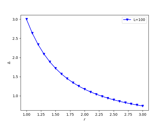
Figure 1: The bulk gap of the model in Eq. (24) as a function of $r$. We performed DMRG for $L=100$.

To establish the existence of a gap in the thermodynamic limit, we study the size dependence of the gap. The exact solution for the (non-interacting) transverse field Ising model shows that the finite size gap converges to its thermodynamic value as $L^{-2}$ in the ordered phase. We checked that for the PE line the gap saturates to its thermodynamic value as $L^{-\alpha}$ where $\alpha$ is very close to $2$.

We numerically determined the gap along the $Z_{3}$ line for different system sizes up to $L=100$. We fitted a power-law function, $\Delta(L)=aL^{-b}+\Delta_{\infty}$ (in analogy with the $Z_{2}$ case). The data and the fitted curve for $r=2.0$ are presented in Fig. 2. The gap decays as $L^{-1.75}$ to its thermodynamic value $\Delta_{\infty}=1.171$. Recent results on the gap of frustration-free models show that if the gap decays to a finite value faster than $L^{-3/2}$, the model is gapped lemm18 , including our model Eq. (24).

As we mentioned above, the error in the energy is of the order $10^{-4}$ in our calculation. The difference between the gap for $L=90$ and $L=100$ is $2\times 10^{-4}$ which shows that the energy has basically converged to its final value within our precision. We also checked that the gap converges to a finite non-zero value with the same behaviour and $b\approx 1.75$ in the range $1.00<r<3.00$.

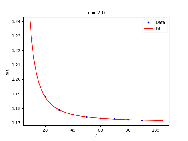
Figure 2: The bulk gap of the model in Eq. (24) as a function of $r$. We performed DMRG for $L=100$. We plot data and the curve $\Delta(L)=3.236L^{-1.751}+1.1706$. The error for each gap point is $10^{-4}$.

We numerically found that the gap decreases as $r$ increases, in analogy to the PE line. As it was pointed out in the previous studiesds03 , in the large $l$ limit of the PE line, where the $U$ and $h$ couplings dominate the Hamiltonian, the PE-line reaches a multicritical point. At this point the ground state degeneracy grows exponentially with the system size. To see this, following Ref.ds03 , we rewrite $h^{PE}_{j,j+1}(l)$ for large $l$,

$$\lim_{l\rightarrow\infty}h^{PE}_{j,j+1}(l)=\frac{e^{l}}{4}\left(\sigma^{z}_{j}+\mathbf{1}\right)\left(\sigma^{z}_{j+1}+\mathbf{1}\right)\ .$$ (56)

For this Hamiltonian any state which does not have two adjacent spins in the $+z$ direction is a ground state, explaining the exponential degeneracy of the ground state with system size.

The same thing happens along the $Z_{3}$ line. In the large $r$ limit we can rewrite the Hamiltonian as

$$\lim_{r\rightarrow\infty}h_{j,j+1}^{Z_{3}}(r) =$$

$$\frac{2}{9}r^{2}\left(\mathbf{1}+Z_{j}+Z^{\dagger}_{j}\right)\left(\mathbf{1}+Z_{j+1}+Z^{\dagger}_{j+1}\right)\ .$$ (57)

Similar to the PE line in this limit any state which does not have two adjacent ”spins” in the $n=0$ state, is a ground state. Therefore we conclude that our model has a multicritical point for $r\rightarrow\infty$.

IV Spin-$S$ Peschel-Emery line

We study the spin-$S$ generalization of the PE-line which has been investigated previously kur82 ; sen91 ; muller85 ; ds03 . Here we present the exact ground states, which again are product states, as well as exact, local edge modes and two exact excited states. The Hamiltonian for this model is

$$\begin{split}h^{\rm S-PE}_{j,j+1}=-S^{x}_{j}S^{x}_{j+1}+\frac{h(l)}{2}S\left(S^{z}_{j}+S^{z}_{j+1}\right)\\ +U(l)S^{z}_{j}S^{z}_{j+1}+S^{2}(U(l)+1)\ ,\end{split}$$ (58)

in which $S^{\alpha}$ are spin-$S$ operators of $SU(2)$. The parameters $U(l)=\dfrac{1}{2}[\cosh(l)-1]$ and $h(l)=\sinh(l)$, are the same as the PE-line couplings in Eq. (2). We note that in the $S=1/2$ case, the Hamiltonian Eq. (58) is $\frac{1}{4}$ times $h^{\rm PE}_{j,j+1}$ (see Eq. (2)), which is written in terms of Pauli operators instead of spin-$1/2$ operators.

The Hamiltonian Eq. (58) commutes with the ‘parity’ of the magnetization, $P_{M}=\prod_{j=1}^{L}e^{i\pi(S-S^{z}_{j})}$, because the operators $S^{x}_{j}S^{x}_{j+1}$ either change the magnetization by two units, or leave it unchanged.

The model has two exactly degenerate ground states for arbitrary $l$, which can be written as product states, similar to the $Z_{2}$ and $Z_{3}$-clock model cases. These two ground states are

$$|\psi_{S,1}(l)\rangle =\left(e^{\alpha S^{-}}|S\rangle_{z}\right)^{\otimes L} |\psi_{S,2}(l)\rangle =\left(e^{-\alpha S^{-}}|S\rangle_{z}\right)^{\otimes L}$$ (59)

where $\alpha=\exp(\frac{l}{2})$ and $|S\rangle_{z}$ is the $S^{z}=S$ eigenstate, i.e. $S^{z}|S\rangle_{z}=S|S\rangle_{z}$. The states $|\psi_{S,1}(l)\rangle$ and $|\psi_{S,2}(l)\rangle$ are not parity eigenstates, but these can be constructed as

$$|E=0;\pm\rangle=(|\psi_{S,1}(l)\rangle\pm|\psi_{S,2}(l)\rangle)/2\ .$$ (60)

As in the previous cases, these states are exact ground states for both the open and periodic chains, with the energy per bond given by $\epsilon_{S}(l)=0$.

Following the $\mathbb{Z}_{2}$ case we can define local edge operators,

$$A_{S}(l) =\frac{1}{2S}(\frac{1}{\alpha}S^{+}_{1}+\alpha S^{-}_{1})$$ (61)

$$B_{S}(l) =-\frac{i}{2S}P_{M}(\frac{1}{\alpha}S^{+}_{L}+\alpha S^{-}_{L})\ .$$ (62)

For $S=1/2$, these operators reduce to $A_{\frac{1}{2}}(l)$ and $B_{\frac{1}{2}}(l)$ in Eq. (7). They act like $S^{z}$ and $-S^{y}$ on the ground states $\{|\psi_{S,1}(l)\rangle,|\psi_{S,2}(l)\rangle\}$.

In the case of periodic boundary conditions, it is possible to write exact excited states of the model Eq. (58). These excited states are constructed from the ground states of the model with two sites as before. The ground states $|g_{\pm}\rangle$ with parities $P_{M}=\pm 1$ of the two site model are obtained by acting on $|S,S\rangle$ as

$$|g_{\pm}\rangle=\left[e^{\alpha(S^{-}_{1}+S^{-}_{2})}\pm e^{-\alpha(S^{-}_{1}+S^{-}_{2})}\right]|S,S\rangle\ .$$ (63)

There are two parity eigenstates $|e_{\pm}\rangle$ with energy $E=S$, which can be obtained from the ground states

$$|e_{\pm}\rangle=(S^{z}_{1}-S^{z}_{2})|g_{\pm}\rangle\ .$$ (64)

We note that we assumed that $S>1/2$ here, because for $S=1/2$, we have $(S^{z}_{1}-S^{z}_{2})|g_{+}\rangle=0$, in agreement with results for the $Z_{2}$ case discussed above.

To find the two exact excited states of the system with length $L=2N$, we first rewrite the ground states of the $L=2N$ site chain in terms of the $g_{\pm}$, similar to Eq. (16)

$$|E=0;\pm\rangle=\sum_{i_{1}\cdots i_{N}=\pm}g_{i_{1}}g_{i_{2}}\dots g_{i_{N-1}}g_{i_{N}}\ ,$$ (65)

where the sum is again over all $2^{N-1}$ configurations $i_{j}=\pm$, with fixed total parity of the magnetization. These states are ground states for both the open and periodic cases, with momentum $K=0$. From these $K=0$ states, one obtains $K=\pi$, parity eigenstates with energy $E=2S$, by replacing the one of ‘$g_{i}$-blocks’ by an ‘$e_{i}$-block’ with the same parity, and summing over the position, again in analogy with the spin-$1/2$ case,

$$|E=2S;\pm\rangle=\sum_{j=1}^{N}(S_{2j-1}^{z}-S_{2j}^{z})|E=0;\pm\rangle\ .$$ (66)

V Discussion

We considered one-dimensional models for which the ground states and a few excited states can be obtained analytically. These models are inspired by the Peschel-Emery linepe81 , of the interacting transverse field Ising model (or, in its fermionic incarnation, Kitaev’s Majorana chain in the presence of a Hubbard interaction). In particular, we constructed a direct analog of the PE-line, starting from the 3-state Clock/Potts model, by introducing two types of additional interaction terms.

For the resulting one-parameter family of models, the three-fold degenerate ground states can be written in product form. In addition, we found a triple of excited states that can be obtained analytically. More importantly, we constructed completely local operators, that permute the parity ground states. These operators almost satisfy the parafermion relations, the only requirement missing is that they are not unitary. Although we believe it should be possible to construct (exponentially) localized parafermion operators, we only succeeded in constructing these for the two-site problem, where they already are quite complicated.

The model studied in this paper behaves in close analogy to the model considered recently by Iemini et al.ma17 . It would be interesting to see if both models can be obtained from a more general model. For instance, it is interesting to notemora-private that the construction of the local operators that permute the ground states can be extended to the model of Ref. ma17, .

In addition to the results for the 3-state clock-type models, we also considered an arbitrary spin-$S$ version of the Peschel-Emery line.

There has been a lot of interest in Clock/Potts type models recently, both the chiral as well as the non-chiral versions. It was only rather recently that the phase-diagram of the chiral 3-state Potts model has been investigated in detailzh15 . The additional ‘interaction’ terms that we needed to consider, namely $Z_{j}Z_{j+1}+{\rm h.c.}$ and $Z_{j}Z^{\dagger}_{j+1}+{\rm h.c.}$ have not attracted much attention yet, but they were considered beforeqin12 ; lahtinen17 in somewhat different contexts. Investigating the phase diagram of the more general model

$$H=\sum_{j}-X_{j}X_{j+1}^{\dagger}+fZ_{j}+gZ_{j}Z_{j+1}+g^{\prime}Z_{j}Z^{\dagger}_{j+1}+{\rm h.c.}$$

would be very interesting, both in the chiral as well as the non-chiral caseburello14 . Finally, it would be interesting to investigate the relation with parafermionic topological phases, which have attracted quite some attention during the recent years, see for instancebondesan ; jf14 ; xu17 .

The interacting transverse field Ising model, Eq. (2) for general $h$ and $U$, is related to the Axial Next-Nearest Neighbour Ising(ANNNI) model, whose phase diagram has been studied thoroughlyselke . Those studies are related to the large $s$ limit of the PE line and its dual version. The phase diagram of ANNNI model is quite rich and has, for instance, an incommensurate phase. As we showed in Sec. III.4, the large $l$ limit of the $Z_{3}$ line also has a multi-critical point. In this light, it would be interesting to study the phase diagram of $Z_{3}$ model and its dual.

Acknowledgments — We would like to thank L. Mazza, C. Mora, N. Regnault and D. Schuricht for interesting discussions. This work was sponsored, in part, by the Swedish Research Council.

Appendix A Exact excited states along the PE-line

In this appendix, we prove that the states Eq. (20), $|E=4,\pm\rangle$, are indeed exact excited states of the Peschel-Emery Hamiltonian for the case with periodic boundary conditions and an even number of sites, $L=2N$. We recall that

$$|E=4,\pm\rangle =O^{-}_{\rm tot}|E=0;\pm\rangle$$

$$=4\mathcal{N}_{\pm}\sum_{j=1}^{N}\sum_{i_{1}\cdots i_{N}=\pm}g_{i_{1}}\cdots g_{i_{j-1}}e_{-}g_{i_{j+1}}\cdots g_{i_{N}}\ .$$

where we introduced the notation $O^{-}_{\rm tot}=\sum_{j=1}^{N}O_{j}^{-}$. We then have that

$$H|E=4,\pm\rangle =HO_{\rm tot}^{-}|E=0,\pm\rangle$$

$$=O_{\rm tot}^{-}H|E=0,\pm\rangle+[H,O_{\rm tot}^{-}]|E=0,\pm\rangle$$

$$=[H,O_{\rm tot}^{-}]|E=0,\pm\rangle\ .$$

It is straightforward to evaluate the commutator

$$[H,O_{\rm tot}^{-}]=-2i\bigl{(} +\sigma_{1}^{x}\sigma^{y}_{2}-\sigma_{1}^{y}\sigma^{x}_{2}$$

$$-\sigma_{2}^{x}\sigma^{y}_{3}+\sigma_{2}^{y}\sigma^{x}_{3}$$

$$\vdots$$

$$-\sigma_{L}^{x}\sigma^{y}_{1}+\sigma_{L}^{y}\sigma^{x}_{1}\bigr{)}\ .$$

To find the action of the commutator on the ground state, we need to know

$$-2i(\sigma_{1}^{x}\sigma^{y}_{2}-\sigma_{1}^{y}\sigma^{x}_{2})|\uparrow\uparrow\rangle =0$$

$$-2i(\sigma_{1}^{x}\sigma^{y}_{2}-\sigma_{1}^{y}\sigma^{x}_{2})|\downarrow\downarrow\rangle =0$$

$$-2i(\sigma_{1}^{x}\sigma^{y}_{2}-\sigma_{1}^{y}\sigma^{x}_{2})|\uparrow\downarrow\rangle =-4|\downarrow\uparrow\rangle$$

$$-2i(\sigma_{1}^{x}\sigma^{y}_{2}-\sigma_{1}^{y}\sigma^{x}_{2})|\downarrow\uparrow\rangle =4|\uparrow\downarrow\rangle,$$

resulting in

$$-2i(\sigma_{1}^{x}\sigma^{y}_{2}-\sigma_{1}^{y}\sigma^{x}_{2})|g_{+}\rangle =0$$

$$-2i(\sigma_{1}^{x}\sigma^{y}_{2}-\sigma_{1}^{y}\sigma^{x}_{2})|g_{-}\rangle =4|e_{-}\rangle\ .$$

This in turn means that

$$H|E=4,\pm\rangle =8\mathcal{N}_{\pm}(\mathbf{1}-T)\times$$

$$\sum_{j=1}^{N}\sum_{i_{1}\cdots i_{N}=\pm}g_{i_{1}}\cdots g_{i_{j-1}}e_{-}g_{i_{j+1}}\cdots g_{i_{N}}$$

where $T$ is the operator that translates the system by one site and we do not sum over $i_{j}$. Because

$$\sum_{j=1}^{N}\sum_{i_{1}\cdots i_{N}=\pm}g_{i_{1}}\cdots g_{i_{j-1}}e_{-}g_{i_{j+1}}\cdots g_{i_{N}}$$

is a state with momentum $K=\pi$, as can be verified directly, it follows that

$$H|E=4,\pm\rangle=4|E=4,\pm\rangle\ ,$$ (67)

which we wanted to show. That the other states given in the main text also are exact excited states can be verified in a similar manner.

Appendix B Two-site parafermion operator

In this appendix, we construct the most general parafermion operator that permutes the three parity ground states Eq. (III.1) of the model Eq. (24), for arbitrary parameter $r>0$. We write this operator in the basis $\{|00\rangle,|01\rangle,|02\rangle,|10\rangle,\ldots,|22\rangle\}$. The operator $O(r)$ we are after should change the sectors as

$$O(r)|E=0;1\rangle =|E=0;\bar{\omega}\rangle$$

$$O(r)|E=0;\omega\rangle =|E=0;1\rangle$$ (68)

$$O(r)|E=0;\bar{\omega}\rangle =|E=0;\omega\rangle\ ,$$

which is how $X_{1}$ acts in the case $r=1$. This means that $O(r)$ should consist of operators of the form $X_{1}$, $X_{2}$, $X_{1}^{\dagger}X_{2}^{\dagger}$, $Z_{1}X_{1}$, etc.. In total, there are 27 such operators. Alternatively, there are 27 non-zero entries in the matrix representation of $O(r)$. We present the operator in terms of the latter. A convenient labeling turns out to be

$$O(r)=\begin{pmatrix}0&b_{2;3}&0&b_{1;3}&0&0&0&0&b_{3;3}\\ 0&0&c_{1;2}&0&c_{3;2}&0&c_{2;2}&0&0\\ a_{3;1}&0&0&0&0&a_{2;1}&0&a_{1;1}&0\\ 0&0&c_{1;1}&0&c_{3;1}&0&c_{2;1}&0&0\\ a_{3;3}&0&0&0&0&a_{2;3}&0&a_{1;3}&0\\ 0&b_{2;2}&0&b_{1;2}&0&0&0&0&b_{3;2}\\ a_{3;2}&0&0&0&0&a_{2;2}&0&a_{1;2}&0\\ 0&b_{2;1}&0&b_{1;1}&0&0&0&0&b_{3;1}\\ 0&0&c_{1;3}&0&c_{3;3}&0&c_{2;3}&0&0\\ \end{pmatrix}\ .$$ (69)

Because it is possible in the $Z_{2}$ case to write the corresponding operator using real parameters, we make the same assumption here. Apart from the conditions Eq. (B), the operator $O$ should satisfy $O(r)^{\dagger}=O(r)$ and $O(r)^{3}=1$. The former condition means that the parameters $a_{i;j}$, $b_{i;j}$ and $c_{i;j}$ form three sets of three orthonormal vectors. So if $\vec{a}_{1}=(a_{1;1},a_{1;2},a_{1;3})^{T}$ etc, we have $\vec{a}_{i}^{T}\cdot\vec{a}_{j}=\delta_{i,j}$ and similar for the other two sets. Each of these three sets is constrained by one of the equations in Eq. (B). In particular, the vectors lie on the intersection of a sphere and a plane; for each set of orthonormal vectors, there are two such planes. The structure of the constraints Eq. (B) is such that their is a solution. In fact, for each set of orthonormal vectors, the solution is parametrized by an angle. Explicitly, these solutions take the form (using the parameters $c=\sqrt{1+2r^{4}}$ and $d=\sqrt{2r^{2}+r^{4}}$)

$$a_{1;1} =\frac{2r^{3}+(cd+r^{2})\cos(\phi_{1})+(-d+cr^{2})\sin(\phi_{1})}{2cd}$$

$$a_{1;2} =\frac{2r^{3}+(-cd+r^{2})\cos(\phi_{1})+(d+cr^{2})\sin(\phi_{1})}{2cd}$$

$$a_{1;3} =-\frac{r(-r^{3}+\cos(\phi_{1})+c\sin(\phi_{1}))}{cd}$$

$$a_{2;1} =\frac{2r^{3}+(-cd+r^{2})\cos(\phi_{1})-(d+cr^{2})\sin(\phi_{1})}{2cd}$$

$$a_{2;2} =\frac{2r^{3}+(cd+r^{2})\cos(\phi_{1})+(d-cr^{2})\sin(\phi_{1})}{2cd}$$

$$a_{2;3} =\frac{r(r^{3}-\cos(\phi_{1})+c\sin(\phi_{1}))}{cd}$$

$$a_{3;1} =\frac{r(1-r^{3}\cos(\phi_{1})+dr\sin(\phi_{1}))}{cd}$$

$$a_{3;2} =-\frac{r(-1+r^{3}\cos(\phi_{1})+dr\sin(\phi_{1}))}{cd}$$

$$a_{3;3} =\frac{r^{2}(1+2r\cos(\phi_{1}))}{cd}$$

$$b_{1;1} =\frac{2r^{3}+(cd+r^{2})\cos(\phi_{2})+(d-cr^{2})\sin(\phi_{2})}{2cd}$$

$$b_{1;2} =\frac{2r^{3}+(-cd+r^{2})\cos(\phi_{2})+(d+cr^{2})\sin(\phi_{2})}{2cd}$$

$$b_{1;3} =-\frac{r(-1+r^{3}\cos(\phi_{2})+dr\sin(\phi_{2}))}{cd}$$

$$b_{2;1} =\frac{2r^{3}+(-cd+r^{2})\cos(\phi_{2})-(d+cr^{2})\sin(\phi_{2})}{2cd}$$

$$b_{2;2} =\frac{2r^{3}+(cd+r^{2})\cos(\phi_{2})+(-d+cr^{2})\sin(\phi_{2})}{2cd}$$

$$b_{2;3} =\frac{r(1-r^{3}\cos(\phi_{2})+dr\sin(\phi_{2}))}{cd}$$

$$b_{3;1} =\frac{r(r^{3}-\cos(\phi_{2})+c\sin(\phi_{2}))}{cd}$$

$$b_{3;2} =-\frac{r(-r^{3}+\cos(\phi_{2})+c\sin(\phi_{2}))}{cd}$$

$$b_{3;3} =\frac{r^{2}(1+2r\cos(\phi_{2}))}{cd}$$

$$c_{1;1} =\frac{r^{2}(1+(1+r^{2})\cos(\phi_{3}))}{d^{2}}$$

$$c_{1;2} =\frac{r^{2}(1-\cos(\phi_{3})+d\sin(\phi_{3}))}{d^{2}}$$

$$c_{1;3} =\frac{r(r^{2}-r^{2}\cos(\phi_{3})-d\sin(\phi_{3}))}{d^{2}}$$

$$c_{2;1} =-\frac{r^{2}(-1+\cos(\phi_{3})+d\sin(\phi_{3}))}{d^{2}}$$

$$c_{2;2} =\frac{r^{2}(1+(1+r^{2})\cos(\phi_{3}))}{d^{2}}$$

$$c_{2;3} =\frac{r(r^{2}-r^{2}\cos(\phi_{3})+d\sin(\phi_{3}))}{d^{2}}$$

$$c_{3;1} =\frac{r(r^{2}-r^{2}\cos(\phi_{3})+d\sin(\phi_{3}))}{d^{2}}$$

$$c_{3;2} =\frac{r(r^{2}-r^{2}\cos(\phi_{3})-d\sin(\phi_{3}))}{d^{2}}$$

$$c_{3;3} =\frac{r^{2}(r^{2}+2\cos(\phi_{3}))}{d^{2}}$$

Finally, the condition $O(r)^{3}=1$ leads to the constraint that $\phi_{1}+\phi_{2}+\phi_{3}=0$. This leaves a two-parameter family of solutions for the operator $O(r)$. There are three rather special solutions, namely $\phi_{1}=\phi_{2}=\phi_{3}=-2\pi/3,0,2\pi/3$. In the limit $r=1$, when the model reduces to $h^{Z_{3}}_{j,j+1}=\bigl{[}-X_{j}X^{\dagger}_{j+1}+{\rm h.c.}\bigr{]}+2$, the operator $O(1)$ becomes $X_{1}$, $X^{\dagger}_{1}X^{\dagger}_{2}$, $X_{2}$ in these three cases respectively. One could hope that the form of $O(r)$ in the two cases $\phi_{1}=\phi_{2}=\phi_{3}=\pm 2\pi/3$ would give a hint for the possible form of two parafermion operators that are exponentially localized at the edges in the case of longer chains. However, the already rather complicated form of this operator in the two-site case makes it hard to guess the general form for larger system sizes.

References

- (1) A.Y. Kitaev, Unpaired Majorana fermions in quantum wires, Phys. Usp. 44, 131 (2001), doi:10.1070/1063-7869/44/10S/S29.
- (2) Y. Oreg, G. Refael, F. von Oppen, Helical Liquids and Majorana Bound States in Quantum Wires, Phys. Rev. Lett. 105, 177002 (2010), doi:10.1103/PhysRevLett.105.177002.
- (3) R.M. Lutchyn, J.D. Sau, S. Das Sarma, Majorana Fermions and a Topological Phase Transition in Semiconductor-Superconductor Heterostructures, Phys. Rev. Lett. 105, 077001 (2010), doi:10.1103/PhysRevLett.105.077001.
- (4) V. Mourik, K. Zuo, S.M. Frolov, S.R. Plissard, E.P.A.M. Bakkers, L.P. Kouwenhoven, Signatures of Majorana Fermions in Hybrid Superconductor-Semiconductor Nanowire Devices, Science 336, 1003 (2012), doi:10.1126/science.1222360.
- (5) M.T. Deng, C.L. Yu, G.Y. Huang, M. Larsson, P. Caroff, H.Q. Xu, Anomalous Zero-Bias Conductance Peak in a Nb-InSb Nanowire-Nb Hybrid Device, Nano Lett. 12, 6414 (2012), doi:10.1021/nl303758w.
- (6) A. Das, Y. Ronen, Y. Most, Y. Oreg, M. Heiblum, H. Shtrikman, Zero-bias peaks and splitting in an Al-InAs nanowire topological superconductor as a signature of Majorana fermions, Nat. Phys. 8, 887 (2012), doi:10.1038/nphys2479.
- (7) A.Y. Kitaev, Fault-tolerant quantum computation by anyons, Ann. Phys. 303, 2 (2003), doi:10.1016/S0003-4916(02)00018-0.
- (8) J. Alicea, P. Fendley, Topological Phases with Parafermions: Theory and Blueprints, Annu. Rev. Cond. Mat. Phys. 7 119 (2016), doi:10.1146/annurev-conmatphys-031115-011336.
- (9) P. Fendley, Strong zero modes and eigenstate phase transitions in the XYZ/interacting Majorana chain, J. Phys. A: Math. Theor. 49, 30LT01 (2016), doi:10.1088/1751-8113/49/30/30LT01.
- (10) P. Fendley, Parafermionic edge zero modes in -invariant spin chains, J. Stat. Mech. (2012) P11020 , doi:10.1088/1742-5468/2012/11/P11020.
- (11) R.S.K. Mong, D.J. Clarke, J. Alicea, N.H. Lindner, P. Fendley, C. Nayak, Y. Oreg, A. Stern, E. Berg, K. Shtengel, M.P.A. Fisher, Universal topological quantum computation from a superconductor/Abelian quantum Hall heterostructure, Phys. Rev. X 4, 011036 (2014), doi:10.1103/PhysRevX.4.011036.
- (12) A. Vaezi, Superconducting analogue of the parafermion fractional quantum Hall states, Phys. Rev. X 4, 031009 (2014), doi:10.1103/PhysRevX.4.031009.
- (13) I. Affleck, T. Kennedy, E.H. Lieb, H. Tasaki, Rigorous results on valence-bond ground states in antiferromagnets, Phys. Rev. Lett. 59, 799 (1987), doi:10.1103/PhysRevLett.59.799.
- (14) I. Affleck, T. Kennedy, E.H. Lieb, H. Tasaki, Valence bond ground states in isotropic quantum antiferromagnets, Commun. Math. Phys. 115, 477 (1988), doi:10.1007/BF01218021.
- (15) C.K. Majumdar, D.K. Ghosh, On Next-Nearest-Neighbor Interaction in Linear Chain. I, J. Math. Phys. 10, 1388 (1969), doi:10.1063/1.1664978.
- (16) C.K. Majumdar, D.K. Ghosh, On Next-Nearest-Neighbor Interaction in Linear Chain. II, J. Math. Phys. 10, 1399 (1969), doi:10.1063/1.1664979.
- (17) I. Peschel, V.J. Emery, Calculation of spin correlations in two-dimensional Ising systems from one-dimensional kinetic models, Z. Phys. B 43, 241 (1981), doi:10.1007/BF01297524.
- (18) I. Peschel, T.T. Truong, The kinetic Potts chain and related potts models with competing interactions, J. Stat. Phys. 45, 233 (1986), doi:10.1007/BF01033089.
- (19) H. Katsura, D. Schuricht, M. Takahashi, Exact ground states and topological order in interacting Kitaev/Majorana chains, Phys. Rev. B 92, 115137 (2015), doi:10.1103/PhysRevB.92.115137.
- (20) P. Jordan, E. Wigner, Über das Paulische Äquivalenzverbot, Z. Physik 47, 631 (1928), doi:10.1007/BF01331938.
- (21) E. Sela, A. Altland, A. Rosch, Majorana fermions in strongly interacting helical liquids, Phys. Rev. B 84, 085114 (2011), doi:10.1103/PhysRevB.84.085114.
- (22) E. Lieb, T. Schultz, D. Mattis, Two soluble models of an antiferromagnetic chain, Ann. Phys. 16, 407 (1961), doi:10.1016/0003-4916(61)90115-4.
- (23) R.J. Elliott, P. Pfeuty, C. Wood, Ising Model with a Transverse Field, Phys. Rev. Lett. 25, 443 (1970), doi:10.1103/PhysRevLett.25.443.
- (24) P. Pfeuty, The one-dimensional Ising model with a transverse field, Ann. Phys. 57, 79 (1970), doi:10.1016/0003-4916(70)90270-8.
- (25) J. Kemp, N.Y. Yao, C.R. Laumann, P. Fendley, Long coherence times for edge spins, J. Stat. Mech. 063105 (2017), doi:10.1088/1742-5468/aa73f0.
- (26) A. Alexandradinata, N. Regnault, C. Fang, M.J. Gilbert, B.A. Bernevig, Parafermionic phases with symmetry breaking and topological order, Phys. Rev. B 94, 125103 (2016), doi:10.1103/PhysRevB.94.125103.
- (27) W.J. Caspers, W. Magnus, Some exact excited states in a linear antiferromagnetic spin system, Phys. Lett. A 88, 103 (1982), doi:10.1016/0375-9601(82)90603-X.
- (28) D.P. Arovas, Two exact excited states for the AKLT chain, Phys. Lett. A 137, 431 (1989), doi:10.1016/0375-9601(89)90921-3.
- (29) S. Moudgalya, S. Rachel, B.A. Bernevig, N. Regnault, Exact Excited States of Non-Integrable Models, arXiv:1708.05021 (unpublished).
- (30) Vl.S. Dotsenko, Critical behaviour and associated conformal algebra of the Potts model, Nucl. Phys. B 235, 54 (1984), doi:10.1016/0550-3213(84)90148-2.
- (31) Y. Zhuang, H.J. Changlani, N.M. Tubman, T.L. Hughes, Phase diagram of the parafermionic chain with chiral interactions, Phys. Rev. B 92, 035154 (2015), doi:10.1103/PhysRevB.92.035154.
- (32) A.S. Jermyn, R.S.K. Mong, J. Alicea, P. Fendley, Stability of zero modes in parafermion chains, Phys. Rev. B 90, 165106 (2014), doi:10.1103/PhysRevB.90.165106.
- (33) N. Moran, D. Pellegrino, J.K. Slingerland, G. Kells, Parafermionic clock models and quantum resonance, Phys. Rev. B 95, 235127 (2017), doi:10.1103/PhysRevB.95.235127.
- (34) A.B. Zamolodchikov, V.A. Fateev, Nonlocal (parafermion) currents in two-dimensional conformal quantum field theory and self-dual critical points in -symmetric statistical systems, Zh. Eksp. Teor. Fiz. 89, 380 (1985), http://jetp.ac.ru/cgi-bin/dn/e_062_02_0215.pdf.
- (35) F. Iemini, C. Mora, L. Mazza, Topological Phases of Parafermions: A Model with Exactly Solvable Ground States, Phys. Rev. Lett. 118 170402 (2017), doi:10.1103/PhysRevLett.118.170402.
- (36) E. Cobanera, G. Ortiz, Fock parafermions and self-dual representations of the braid group, Phys. Rev. A 89 012328 (2014), doi:10.1103/PhysRevA.89.012328.
- (37) H. Katsura, talk at the first annual meeting of Topological Materials Science, Kyoto, December 2015.
- (38) E. Fradkin, L.P. Kadanoff, Disorder variables and para-fermions in two-dimensional statistical mechanics, Nucl. Phys. B 170 1 (1980), doi:10.1016/0550-3213(80)90472-1.
- (39) S.R. White, Density matrix formulation for quantum renormalization groups, Phys. Rev. Lett. 69, 2863 (1992), doi:10.1103/PhysRevLett.69.2863.
- (40) U. Schollwöck, The density-matrix renormalization group, Rev. Mod. Phys. 77, 259 (2005), doi:10.1103/RevModPhys.77.259.
- (41) F. Albuquerque, F. Alet, P. Corboz, P. Dayal, A. Feiguin, S. Fuchs, L. Gamper, E. Gull, S. Gürtler, A. Honecker, R. Igarashi, M. Körner, A. Kozhevnikov, A. Läuchli, S.R. Manmana, M. Matsumoto, I.P. McCulloch, F. Michel, R.M. Noack, G. Pawlowski, L. Pollet, T. Pruschke, U. Schollwöck, S. Todo, S. Trebst, M. Troyer, P. Werner, S. Wessel, and for the ALPS collaboration, The ALPS project release 1.3: Open-source software for strongly correlated systems, J. Magn. Magn. Mater. 310, 1187 (2007), doi:10.1016/j.jmmm.2006.10.304.
- (42) B. Bauer, L.D. Carr, H.G. Evertz, A. Feiguin, J. Freire, S. Fuchs, L. Gamper, J. Gukelberger, E. Gull, S. Güertler, A. Hehn, R. Igarashi, S.V. Isakov, D. Koop, P.N. Ma, P. Mates, H. Matsuo, O. Parcollet, G. Pawlowski, J.D. Picon, L. Pollet, E. Santos, V.W. Scarola, U. Schollwöck, C. Silva, B. Surer, S. Todo, S. Trebst, M. Troyer, M.L. Wall, P. Werner, S. Wessel, The ALPS project release 2.0: open source software for strongly correlated systems, J. Stat. Mech (2011) P05001, doi:10.1088/1742-5468/2011/05/P05001.
- (43) M. Dolfi, B. Bauer, S. Keller, A. Kosenkov, T. Ewart, A. Kantian, T. Giamarchi, M. Troyer, Matrix product state applications for the ALPS project, Comput. Phys. Commun. 185, 3430 (2014), doi:10.1016/j.cpc.2014.08.019.
- (44) M. Lemm, E. Mozgunov, Spectral gaps of frustration-free spin systems with boundary, arXiv:1801.08915 (unpublished).
- (45) A. Dutta, D. sen, Gapless line for the anisotropic Heisenberg spin chain in a magnetic field and the quantum axial next-nearest-neighbor Ising chain, Phys. Rev. B 67, 094435 (2003), doi:10.1103/PhysRevB.67.094435.
- (46) J. Kurmann, H. Thomas, G. Müller, Antiferromagnetic long-range order in the anisotropic quantum spin chain, Physica A 112, 235 (1982), doi:10.1016/0378-4371(82)90217-5.
- (47) G. Müller, R.E. Schrock, Implications of direct-product ground states in the one-dimensional quantum XYZ and XY spin chains, Phys. Rev. B 32, 5845 (1985), doi:10.1103/PhysRevB.32.5845.
- (48) D. Sen, Large-S analysis of a quantum axial next-nearest-neighbor Ising model in one dimension, Phys. Rev. B 43, 5939 (1991), doi:10.1103/PhysRevB.43.5939.
- (49) Private discussion with C. Mora.
- (50) M.P. Qin, J.M. Leinaas, S. Ryu, E. Ardonne, T. Xiang, D.-H. Lee, Quantum torus chain, Phys. Rev. B 86, 134430 (2012), doi:10.1103/PhysRevB.86.134430.
- (51) V. Lahtinen, T. Månsson, E. Ardonne, Quantum criticality in many-body parafermion chains, arXiv:1709.04259 (unpublished).
- (52) A. Milsted, E. Cobanera, M. Burrello, G. Ortiz Commensurate and incommensurate states of topological quantum matter, Phys. Rev. B 90, 195101 (2014), doi:10.1103/PhysRevB.90.195101.
- (53) R. Bondesan, T. Quella, Topological and symmetry broken phases of parafermions in one dimension, J. Stat. Mech, P10024 (2013), doi:10.1088/1742-5468/2013/10/P10024.
- (54) W.-T. Xu, G.-M. Zhang, Matrix product states for topological phases with parafermions, Phys. Rev. B 95, 195122 (2017), doi:10.1103/PhysRevB.95.195122.
- (55) W. Selke, The ANNNI model – Theoretical analysis and experimental application, Phys. Rep. 170, 213 (1988), doi:10.1016/0370-1573(88)90140-8.