Bipartitioning Problems on Graphs with Bounded Tree-Width

Abstract

For an undirected graph $G$, we consider the following problems: given a fixed graph $H$, can we partition the vertices of $G$ into two non-empty sets $A$ and $B$ such that neither the induced graph $G[A]$ nor $G[B]$ contain $H$ (i) as a subgraph? (ii) as an induced subgraph? These problems are NP-complete and are expressible in monadic second order logic (MSOL). The MSOL formulation, together with Courcelle’s theorem implies linear time solvability on graphs with bounded tree-width. This approach yields algorithms with running time $f(|\varphi|,t)\cdot n$, where $|\varphi|$ is the length of the MSOL formula, $t$ is the tree-width of the graph and $n$ is the number of vertices of the graph. The dependency of $f(|\varphi|,t)$ on $|\varphi|$ can be as bad as a tower of exponentials.

In this paper, we present explicit combinatorial algorithms for these problems for graphs $G$ whose tree-width is bounded. We obtain $2^{O(t^{r})}\cdot n$ time algorithms when $H$ is any fixed graph of order $r$. In the special case when $H=K_{r}$, a complete graph on $r$ vertices, we get an $2^{O(t+r\log t)}\cdot n$ time algorithm.

The techniques can be extended to provide FPT algorithms to determine the smallest number $q$ such that $V$ can be partitioned into $q$ parts such that none of the parts have $H$ as a subgraph (induced subgraph).

1 Introduction

Let $G=(V,E)$ be an undirected graph on $n$ vertices. In the classical $k$-coloring problem, we need to color the vertices of the graph using at most $k$ colors such that no pair of adjacent vertices are of the same color. The $k$-coloring problem is NP-complete for $k\geq 3$ and this problem, and its variants, have been studied extensively under various settings. For $k=2$, this is equivalent to testing whether the graph is bipartite or not, which is of course solvable in polynomial time.

We consider the following generalization of the 2-coloring problem: we need to $2$-color the vertices of the graph such that the subgraphs induced by the respective color classes do not have a fixed graph $H$ as a subgraph. We call this problem the Bipartitioning without Subgraph $H$ Problem or BWS-$H$ Problem in short.

BWS-$H$ Problem
Instance: An undirected graph $G=(V,E)$.
Question: Can $V$ be partitioned into two non-empty sets $A,B$ such that neither of the induced graphs $G[A]$ and $G[B]$ have $H$ as a subgraph?

We also study the variant of the problem where $H$ does not appear as an induced subgraph. We call this the $H$-Free Bipartitioning Problem.

$H$-Free Bipartitioning Problem
Instance: An undirected graph $G=(V,E)$.
Question: Can $V$ be partitioned into two non-empty sets $A,B$ such that neither of the induced graphs $G[A]$ and $G[B]$ have $H$ as an induced subgraph?

The BWS-$H$ problem is NP-complete [1] unless $H=K_{2}$. Recently, Karpiński [2] gave an alternate proof for the NP-completeness of the problem when $H=C_{r}$, a cycle of fixed length $r$. The $H$-Free Bipartitioning Problem is NP-complete [3] as long as $H$ has $3$ or more vertices. For fixed $H$, both these problems can be expressed in monadic second order logic (MSOL). The well-known Courcelle’s theorem [4, 5] states that any graph property that is expressible in MSOL is solvable in linear time for graphs with bounded tree-width. The resulting algorithms have a running time $f(|\varphi|,t)\cdot n$, where $|\varphi|$ is the length of the MSOL formula and $t$ is the tree-width of the graph. Even though the algorithms run in linear time, the dependency of $f$ on $|\varphi|$ and $t$ can be quite bad. Indeed in the worst case $f(|\varphi|,t)$ can be a tower of exponentials. Considering this, it is preferable to have explicit combinatorial algorithms, since such algorithms are more efficient and are amenable to a precise running time analysis.

In this paper, we give combinatorial algorithms for both BWS-$H$ and $H$-Free Bipartitioning problems. Our main result is the following:

Theorem 1.1

There are $2^{O(t^{r})}\cdot n$ time algorithms that solves the BWS-$H$ and $H$-Free Bipartitioning problems for any arbitrary fixed $H$ ($|V(H)|=r$), on graphs with tree-width at most $t$.

We also obtain a much faster $2^{O(t+r\log t)}\cdot n$ time algorithm when $H=K_{r}$, a complete graph on $r$ vertices. Note that in this case, the BWS-$H$ problem and $H$-Free Bipartitioning problem coincide.

Graph bipartitioning with other constraints have been explored in the past. The degree bounded bipartitioning problem asks to partition the vertices of $G$ into two sets $A$ and $B$ such that the maximum degree in the induced subgraphs $G[A]$ and $G[B]$ are at most $a$ and $b$ respectively. Xiao and Nagamochi [6] proved that this problem is NP-complete for any non-negative integers $a$ and $b$ except for the case $a=b=0$, in which case the problem is equivalent to testing whether $G$ is bipartite. Other variants that place constraints on the degree of the vertices within the partitions have also been studied [7, 8]. Wu, Yuan and Zhao [9] showed the NP-completeness of the variant that asks to partition the vertices of the graph $G$ into two sets such that both the induced graphs are acyclic. A generalization of the $H$-Free Bipartitioning problem called $H$-Free $q$-Coloring has been mentioned in [10].

Farrugia [1] showed the NP-completeness of a general variant of the problems called $(\mathcal{P},\mathcal{Q})$-coloring problem. Here, $\mathcal{P}$ and $\mathcal{Q}$ are any additive induced-hereditary graph properties. The problem asks to partition the vertices of $G$ into $A$ and $B$ such that $G[A]$ and $G[B]$ have properties $\mathcal{P}$ and $\mathcal{Q}$ respectively.

2 Preliminaries

We write $f(n)=O^{*}(g(n))$ if $f(n)=O(g(n)n^{c})$ for some constant $c>0$. Let $G=(V,E)$ be an undirected graph. For $u\in V$, the set of all neighbors of $u$ (open neighborhood) is denoted by $N(u)$. The closed neighborhood of $u$, denoted by $N[u]$, is defined as $N[u]=N(u)\cup\{u\}$. For a vertex set $S\subseteq V$, the subgraph induced by $S$ is denoted by $G[S]$. When there is no ambiguity, we use the simpler notations $S\backslash x$ to denote $S\backslash\{x\}$ and $S\cup x$ to denote $S\cup\{x\}$. We denote the set of all $k$ sized subsets of the set $S$ by $\binom{S}{k}$. We use $uv$ to denote the edge $\{u,v\}$ for convenience. We follow the standard graph theoretic terminology from [11].

A parameterized problem is a language $L\subseteq\Sigma^{*}\times\mathbb{N}$, where $\Sigma$ is a fixed and finite alphabet. For $(x,k)\in\Sigma^{*}\times\mathbb{N}$, $k$ is referred to as the parameter. A parameterized problem $L$ is fixed parameter tractable (FPT) if there is an algorithm $A$, a computable non-decreasing function $f:\mathbb{N}\rightarrow\mathbb{N}$ and a constant $c$ such that, given $(x,k)\in\Sigma^{*}\times\mathbb{N}$ the algorithm $A$ correctly decides whether $(x,k)\in L$ in time bounded by $f(k).|x|^{c}$. For more details on parameterized algorithms refer to [12].

A tree decomposition of $G$ is a pair $(T,\{X_{i},i\in I\})$, where for $i\in I$, $X_{i}\subseteq V$ (usually called bags) and $T$ is a tree with elements of $I$ as the nodes such that:

1. For each vertex $v\in V$, there is an $i\in I$ such that $v\in X_{i}$.

2. For each edge $\{u,v\}\in E$, there is an $i\in I$ such that $\{u,v\}\subseteq X_{i}$.

3. For each vertex $v\in V$, $T[\{i\in I|v\in X_{i}\}]$ is connected.

The width of the tree decomposition is $\max_{i\in I}(|X_{i}|-1)$. The tree-width of $G$ is the minimum width taken over all tree decompositions of $G$ and we denote it as $t$. For more details on tree-width, we refer the reader to [13]. A rooted tree decomposition is called a nice tree decomposition, if every node $i\in I$ is one of the following types:

1. Leaf node: For a leaf node $i$, $X_{i}=\emptyset$.

2. Introduce Node: An introduce node $i$ has exactly one child $j$ and there is a vertex $v\in V\backslash X_{j}$ such that $X_{i}=X_{j}\cup\{v\}$.

3. Forget Node: A forget node $i$ has exactly one child $j$ and there is a vertex $v\in V\backslash X_{i}$ such that $X_{j}=X_{i}\cup\{v\}$.

4. Join Node: A join node $i$ has exactly two children $j_{1}$ and $j_{2}$ such that $X_{i}=X_{j_{1}}=X_{j_{2}}$.

The notion of nice tree decomposition was introduced by Kloks [14]. Every graph $G$ has a nice tree decomposition with $|I|=O(n)$ nodes and width equal to the tree-width of $G$. Moreover, such a decomposition can be found in linear time if the tree-width is bounded.

2.1 Overview of the Techniques Used

In the rest of the paper, we assume that the nice tree decomposition is given. Let $i$ be a node in the nice tree decomposition, $X_{i}$ is the bag of vertices associated with the node $i$. Let $T_{i}$ be the subtree rooted at the node $i$, $G[T_{i}]$ denote the graph induced by all the vertices in $T_{i}$.

We use dynamic programming on the nice tree decomposition to solve the problems for different $H$. We process the nodes of nice tree decomposition according to its post order traversal. We say that a partition $A,B$ of $G$ is a valid partition if neither $G[A]$ nor $G[B]$ have $H$ as a subgraph. At each node $i$, we check each bipartition $(A_{i},B_{i})$ of the bag $X_{i}$ to see if $(A_{i},B_{i})$ leads to a valid partition in the graph $G[T_{i}]$. For each partition, we also keep some extra information that will help us to detect if the partition leads to an invalid partition at some ancestral (parent) node. We have four types of nodes in the tree decomposition – leaf, introduce, forget and join nodes. In the algorithm, we explain the procedure for updating the information at each of these above types of nodes and consequently, to certify whether a partition is valid or not.

In Section 3, we discuss algorithm for the case $H=K_{r}$, a complete graph on $r$ vertices. In Section 4, we discuss algorithm for the BWS-$H$ problem when $H=C_{4}$, a cycle of length $4$. In Section 5, the algorithm for the BWS-$H$ problem for a fixed arbitrary graph $H$ is presented. Presenting algorithms for $H=K_{r}$ and $H=C_{4}$ initially will help in the exposition, as they will help to understand the setup before moving to the more involved generalized case. Finally, we explain how the algorithm for the $H$-Free Bipartitioning problem can be obtained by modifying the algorithm for the BWS-$H$ problem in Section 6.

3 Bipartitioning without $K_{r}$

We consider the BWS-$H$ problem when $H=K_{r}$, a complete graph on $r$ vertices.

Let $\Psi=(A_{i},B_{i})$ be a partition of a bag $X_{i}$. We set $M_{i}[\Psi]$ to $1$ if there exist a partition $(A,B)$ of $V[T_{i}]$ such that $A_{i}\subseteq A$, $B_{i}\subseteq B$ and both $G[A]$ and $G[B]$ are $K_{r}$-free. Otherwise, $M_{i}[\Psi]$ is set to $0$.

Leaf node: For a leaf node $\Psi=(\emptyset,\emptyset)$ and $M_{i}[\Psi]=1$.

Introduce node: Let $j$ be the only child of the node $i$. Suppose, $v\in X_{i}$ is the new vertex present in $X_{i}$, $v\notin X_{j}$. Let $\Psi=(A_{i},B_{i})$ be a partition of $X_{i}$. If $G[A_{i}]$ or $G[B_{i}]$ has $K_{r}$ as a subgraph, we set $M_{i}[\Psi]$ to $0$. Otherwise, we use the following cases to compute $M_{i}[\Psi]$ value. Since $v$ cannot have forgotten neighbors, it can form a $K_{r}$ only within the bag $X_{i}$.

Case 1:

$v\in A_{i}$, $M_{i}[\Psi]=M_{j}[\Psi^{\prime}]$, where $\Psi^{\prime}=(A_{i}\backslash v,B_{i})$.

Case 2:

$v\in B_{i}$, $M_{i}[\Psi]=M_{j}[\Psi^{\prime}]$, where $\Psi^{\prime}=(A_{i},B_{i}\backslash v)$.

Forget node: Let $j$ be the only child of the node $i$. Suppose, $v\in X_{j}$ is the vertex missing in $X_{i}$, $v\notin X_{i}$. Let $\Psi=(A_{i},B_{i})$ be a partition of $X_{i}$. If $G[A_{i}]$ or $G[B_{i}]$ has $K_{r}$ as a subgraph, we set $M_{i}[\Psi]$ to $0$. Otherwise, $M_{i}[\Psi]=\max\{M_{j}[\Psi^{\prime}],M_{j}[\Psi^{\prime\prime}]\}$, where, $\Psi^{\prime}=(A_{i}\cup v,B_{i})$ and $\Psi^{\prime\prime}=(A_{i},B_{i}\cup v)$.

Join node: Let $j_{1}$ and $j_{2}$ be the children of the node $i$. $X_{i}=X_{j_{1}}=X_{j_{2}}$ and $V(T_{j_{1}})\cap V(T_{j_{2}})=X_{i}$. Let $\Psi=(A_{i},B_{i})$ be a partition of $X_{i}$. If $G[A_{i}]$ or $G[B_{i}]$ has $K_{r}$ as a subgraph, we set $M_{i}[\Psi]$ to $0$. Otherwise, we use the following expression to compute $M_{i}[\Psi]$ value. Since there are no edges between $V(T_{j_{1}})\backslash X_{i}$ and $V(T_{j_{2}})\backslash X_{i}$, a $K_{r}$ cannot contain forgotten vertices from both $T_{j_{1}}$ and $T_{j_{2}}$.

$$M_{i}[\Psi]=\left\{\begin{aligned} &1,&\hbox{If $M_{j_{1}}[\Psi]=1$ and $M_{j_{2}}[\Psi]=1$.}\\ &0,&\hbox{Otherwise.}\end{aligned}\right.$$

Correctness of the algorithm implied from the correctness of $M_{i}[\Psi]$ values, which can be proved using bottom up induction on nice tree decomposition. $G$ has a valid bipartitioning if there exists a $\Psi$ such that $M_{r}[\Psi]=1$, where $r$ is the root node of the nice tree decomposition. The total time complexity of the algorithm is $2^{t}t^{r}n=O^{*}(2^{t+r\log t})$. With this we state the following theorem.

Theorem 3.1

There is an $O(2^{t+r\log t}n)$ time algorithm that solves the BWS-$H$ problem when $H=K_{r}$, on graphs with tree-width at most $t$.

4 Bipartitioning without $C_{4}$

In this section, we describe the combinatorial algorithm for the BWS-$H$ problem for the case when $H=C_{4}$, a cycle of length $4$. As stated, the problem can be expressed in MSOL. An MSOL formulation of the BWS-$H$ problem for the case $H=C_{4}$ is given below.

$$\exists V_{1}\subseteq V:\exists V_{2}\subseteq V:(V_{1}\cap V_{2}=\emptyset)\wedge(V_{1}\cup V_{2}=V)\wedge\neg(V_{1}=\emptyset)\wedge\neg(V_{2}=\emptyset)\wedge$$

$$\neg(\exists u_{1}\in V_{1}:\exists u_{2}\in V_{1}:\exists u_{3}\in V_{1}:\exists u_{4}\in V_{1}:$$

$$(u_{1}u_{2}\in E)\wedge(u_{2}u_{3}\in E)\wedge(u_{3}u_{4}\in E)\wedge(u_{4}u_{1}\in E))\wedge$$

$$\neg(\exists u_{1}\in V_{2}:\exists u_{2}\in V_{2}:\exists u_{3}\in V_{2}:\exists u_{4}\in V_{2}:$$

$$(u_{1}u_{2}\in E)\wedge(u_{2}u_{3}\in E)\wedge(u_{3}u_{4}\in E)\wedge(u_{4}u_{1}\in E)).$$

The predicates $V_{1}\cap V_{2}=\emptyset$, $V_{1}\cup V_{2}=V$ and $V_{1}=\emptyset$ can be rewritten as follows:

$$V_{1}\cap V_{2}=\emptyset\Longleftrightarrow\neg\exists v\in V:v\in V_{1}\wedge v\in V_{2},$$

$$V_{1}\cup V_{2}=V\Longleftrightarrow\forall v\in V:v\in V_{1}\vee v\in V_{2},$$

$$V_{1}=\emptyset\Longleftrightarrow\forall v\in V:\neg(v\in V_{1}).$$

Note that a cycle of length $4$ is formed when a pair of (adjacent or non-adjacent) vertices have two or more common neighbors. If a graph has no $C_{4}$ then any vertex pair can have at most one common neighbor. Let $X_{i}$ be a bag at the node $i$ of the nice tree decomposition. We guess a partition $(A_{i},B_{i})$ of the bag $X_{i}$. For each pair of vertices from $A_{i}$ (similarly $B_{i}$), we also guess if the pair has exactly one common forgotten neighbor in part $A$ (similarly $B$) of the partition. We check if the above guesses lead to a valid partitioning in the subgraph $G[T_{i}]$, which is the graph induced by the vertices in the node $i$ and all its descendent nodes. Below we formally explain the technique.

Let $\Psi=(A_{i},B_{i},P_{i},Q_{i})$ be a $4$-tuple defined as follows: $(A_{i},B_{i})$ is a partition of $X_{i}$, $P_{i}\subseteq\binom{A_{i}}{2}$ and $Q_{i}\subseteq\binom{B_{i}}{2}$. Intuitively, $P_{i}$ and $Q_{i}$ are the set of those pairs that have exactly one common forgotten neighbor.

We define $M_{i}[\Psi]$ to be $1$ if there is a partition $(A,B)$ of $V(T_{i})$ such that:

1. $A_{i}\subseteq A$ and $B_{i}\subseteq B$.

2. Every pair in $P_{i}$ has exactly one common neighbor in $A\backslash A_{i}$.

3. Every pair in $\binom{A_{i}}{2}\setminus P_{i}$ does not have a common neighbor in $A\backslash A_{i}$.

4. Every pair in $Q_{i}$ has exactly one common neighbor in $B\backslash B_{i}$.

5. Every pair in $\binom{B_{i}}{2}\setminus Q_{i}$ does not have a common neighbor in $B\backslash B_{i}$.

6. $G[A]$ and $G[B]$ do not have $C_{4}$ as a subgraph.

Otherwise, $M_{i}[\Psi]$ is set to $0$. Suppose there exists a 4-tuple $\Psi$ such that $M_{r}[\Psi]=1$, where $r$ is the root of the nice tree decomposition. Then the above conditions 1 and 6 ensure that $G$ can be partitioned in the required manner.

When one of the following occurs, it is easy to see that the 4-tuple does not lead to a required partition. We say that the 4-tuple $\Psi$ is invalid if one of the below cases occur:

1. $G[A_{i}]$ or $G[B_{i}]$ contains a $C_{4}$.

2. There exists a pair $\{x,y\}$ $\in$ $P_{i}$ with a common neighbor in $A_{i}$.

3. There exists a pair $\{x,y\}$ $\in$ $Q_{i}$ with a common neighbor in $B_{i}$.

Note that it is easy to check if a given $\Psi$ is invalid. Below we explain how to compute $M_{i}[\Psi]$ value at each node $i$.

Leaf node: For a leaf node $i$, $\Psi=(\emptyset,\emptyset,\emptyset,\emptyset)$ and $M_{i}[\Psi]=1$.

Introduce node: Let $j$ be the only child of the node $i$. Suppose $v\in X_{i}$ is the new vertex present in $X_{i}$, $v\notin X_{j}$. Let $\Psi=(A_{i},B_{i},P_{i},Q_{i})$ be a $4$-tuple of $X_{i}$, If $\Psi$ is invalid, we set $M_{i}[\Psi]$ to $0$. Otherwise, we use the following cases to compute the $M_{i}[\Psi]$ value.

Case 1, $v\in A_{i}$:

If $\exists\{v,x\}\in P_{i}$ for some $x\in A_{i}$ or if $\exists\{x,y\}\in P_{i}$ such that $\{x,y\}\subseteq N(v)\cap A_{i}$, then $M_{i}[\Psi]=0$. Otherwise, $M_{i}[\Psi]=M_{j}[\Psi^{\prime}]$, where $\Psi^{\prime}=(A_{i}\backslash v,B_{i},P_{i},Q_{i})$.

As $v$ is a newly introduced vertex, it cannot have any forgotten neighbors. Hence, $\{v,x\}\in P_{i}\Longrightarrow M_{i}[\Psi]=0$. If $x$ and $y$ have a common forgotten neighbor, they all form a $C_{4}$, together with $v$. Hence $\{x,y\}\in P_{i}\Longrightarrow M_{i}[\Psi]=0$.

Case 2, $v\in B_{i}$:

If $\exists\{v,x\}\in Q_{i}$ for some $x\in B_{i}$ or if $\exists\{x,y\}\in Q_{i}$ such that $\{x,y\}\subseteq N(v)\cap B_{i}$, then $M_{i}[\Psi]=0$.. Otherwise, $M_{i}[\Psi]=M_{j}[\Psi^{\prime}]$, where $\Psi^{\prime}=(A_{i},B_{i}\backslash v,P_{i},Q_{i})$.

Forget node: Let $j$ be the only child of the node $i$. Suppose $v\in X_{j}$ is the vertex missing in $X_{i}$, $v\notin X_{i}$. Let $\Psi=(A_{i},B_{i},P_{i},Q_{i})$ be a $4$-tuple of $X_{i}$, If $\Psi$ is invalid, we set $M_{i}[\Psi]$ to $0$. Otherwise, $M_{i}[\Psi]$ is computed as follows:

Case 1, $v\in A_{j}$:

If $\exists x,y\in A_{i}$ such that $xv,yv\in E$, then $v$ is a common forgotten neighbor for $x$ and $y$. Hence we set $M_{i}[\Psi]=0$ whenever $\{x,y\}\notin P_{i}$. Otherwise, let $R=\{\{x,y\}|x,y\in A_{i}\cap N(v)\}$. At node $j$, note that any pair in $R$ with a common forgotten neighbor will form a $C_{4}$. Hence we consider only those $P_{j}$’s that are disjoint with $R$. Also there can be new pairs formed with $v$ at the node $j$. Let $S=\{\{v,x\}|x\in A_{i}\}$. We have the following equation.

$$\delta_{1}=\max_{X\subseteq S}\{M_{j}[A_{i}\cup v,B_{i},(P_{i}\backslash R)\cup X,Q_{i}]\}.$$

Case 2, $v\in B_{j}$:

This is analogous to Case 1. We set $M_{i}[\Psi]=0$, whenever $\{x,y\}\notin Q_{i}$. Otherwise, let $R=\{\{x,y\}|x,y\in B_{i}\cap N(v)\}$ and $S=\{\{v,x\}|x\in B_{i}\}$.

$$\delta_{2}=\max_{X\subseteq S}\{M_{j}[A_{i},B_{i}\cup v,P_{i},(Q_{i}\backslash R)\cup X]\}.$$

If $M_{i}[\Psi]$ is not set to $0$ already, we set $M_{i}[\Psi]=\max\{\delta_{1},\delta_{2}\}$.

Join node: Let $j_{1}$ and $j_{2}$ be the children of the node $i$. By the property of nice tree decomposition, we have $X_{i}=X_{j_{1}}=X_{j_{2}}$ and $V(T_{j_{1}})\cap V(T_{j_{2}})=X_{i}$. There are no edges between $V(T_{j_{1}})\backslash X_{i}$ and $V(T_{j_{2}})\backslash X_{i}$. Let $\Psi=(A_{i},B_{i},P_{i},Q_{i})$ be a $4$-tuple of $X_{i}$. If $\Psi$ is invalid, we set $M_{i}[\Psi]$ to $0$. Otherwise, we use the following expression to compute the value of $M_{i}[\Psi]$.

A pair $\{x,y\}\in P_{i}$ can come either from the left subtree or from the right subtree but not from both, for that would imply two distinct common neighbors for $x$ and $y$ and hence a $C_{4}$. For $X\subseteq P_{i}$ and $Y\subseteq Q_{i}$, $\Psi_{1}=(A_{i},B_{i},X,Y)$ and $\Psi_{2}=(A_{i},B_{i},P_{i}\backslash X,Q_{i}\backslash Y)$.

$$M_{i}[\Psi]=\left\{\begin{aligned} &1,&\hbox{$\exists X\subseteq P_{i},Y\subseteq Q_{i}$ such that $M_{j_{1}}[\Psi_{1}]=M_{j_{2}}[\Psi_{2}]=1$.}\\ &0,&\hbox{Otherwise.}\end{aligned}\right.$$

The correctness of the algorithm is implied by the correctness of $M_{i}[\Psi]$ values, which follows by a bottom-up induction on the nice tree decomposition. $G$ has a valid bipartitioning if there exists a 4-tuple $\Psi$ such that $M_{r}[\Psi]=1$, where $r$ is the root of the nice tree decomposition.

The time complexity at each of the nodes in the tree decomposition is as follows: constant time at leaf nodes, $O^{*}(2^{t+t^{2}})$ time at insert nodes, $O^{*}(2^{2t+t^{2}})$ time at forget nodes and $O^{*}(2^{t+2t^{2}})$ time at join nodes. This gives the following:

Theorem 4.1

There is an $O(2^{O(t^{2})}\dot{n})$ time algorithm that solves the BWS-$H$ Problem when $H=C_{4}$ on graphs with tree-width at most $t$.

5 Bipartitioning without $H$

Let $X_{i}$ be a bag at node $i$ of the nice tree decomposition. Let $(A_{i},B_{i})$ be a partition of $X_{i}$. We can easily check if $G[A_{i}]$ or $G[B_{i}]$ has $H$ as a subgraph. Otherwise, we need to see if there is a partition $(A,B)$ of $V(T_{i})$ such that $A_{i}\subseteq A$, $B_{i}\subseteq B$ and both $G[A_{i}]$ and $G[B_{i}]$ do not have $H$ has a subgraph. If there is such a partition $(A,B)$, then $G[A]$ and $G[B]$ may have subgraph $H^{\prime}$, an induced subgraph of $H$ which can lead to $H$ at some ancestral node (introduce node or join node) of the nice tree decomposition (See Figures 2 and 3).

Figure 1: An example graph $H$.

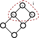
Figure 2: Forming $H$ at an introduce node. Sequence $s=(v,v2,v1,fg,fg,fg)$.

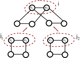
Figure 3: Forming $H$ at join node. Sequences at node $j_{1}$ $s^{\prime}=(dc,dc,v1,v2,fg,fg)$, at node $j_{2}$ $s^{\prime\prime}=(fg,fg,v1,v2,dc,dc)$ gives a sequence $s=(fg,fg,v1,v2,fg,fg)$ at node $i$. Vertices outside the dashed lines are forgotten vertices.

We perform dynamic programming over the nice tree decomposition. At each node $i$ we guess a partition $(A_{i},B_{i})$ of $X_{i}$ and possible induced subgraphs of $H$ that are part of $A$ and $B$ respectively. We check if such a partition is possible. Below we explain the algorithm in detail.

Let the vertices of the graph $H$ are labeled as $u_{1},u_{2},u_{3},\dots,u_{r}$. Let $(A_{i},B_{i})$ be a partition of vertices in the bag $X_{i}$. Let $(A,B)$ be a partition of $V(T_{i})$ such that $A\supseteq A_{i}$ and $B\supseteq B_{i}$. We define $\Gamma_{A_{i}}$ as follows:

$$S_{A_{i}}= \{(w_{1},w_{2},w_{3},\dots,w_{r})|w_{\ell}\in\{A_{i}\cup\{fg,dc\}\},$$

$$\forall\ell_{1}\neq\ell_{2},w_{\ell_{1}}=w_{\ell_{2}}\Longrightarrow w_{\ell_{1}}\in\{fg,dc\}\}.$$

$$I_{A_{i}}= \{s=(w_{1},w_{2},w_{3},\dots,w_{r})\in S_{A_{i}}|\mbox{ there exists }\ell_{1}\neq\ell_{2}$$

$$\mbox{ such that }w_{\ell_{1}}=fg,w_{\ell_{2}}=dc\mbox{ and }\{u_{\ell_{1}},u_{\ell_{2}}\}\in E(H)\}$$

$$\Gamma_{A_{i}}= S_{A_{i}}\backslash I_{A_{i}}$$

Here $fg$ represents a vertex in $A\backslash A_{i}$, the forgotten vertices in $A$ and $dc$ stands for don’t care. That is we don’t care if the corresponding vertex is part of the subgraph or not. Similarly, we can define $\Gamma_{B_{i}}$ with respect to the sets $B_{i}$ and $B$.

A sequence in $S_{A_{i}}$ corresponds to a subgraph $H^{\prime}$ of $H$ in $A$ as follows:

1. If $w_{\ell}=fg$ then $u_{\ell}$ is part of $A\backslash A_{i}$, the forgotten vertices in $A$.

2. If $w_{\ell}=dc$ then $u_{\ell}$ need not be part of the subgraph $H^{\prime}$.

3. If $w_{\ell}\in A_{i}$ then the vertex $w_{\ell}$ corresponds to the vertex $u_{\ell}$ of $H^{\prime}$.

$\Gamma_{A_{i}}$ is the set of sequences that can become $H$ in future at some ancestral (insert/join) node of the tree decomposition. Note that the sequences $I_{A_{i}}$ are excluded from $\Gamma_{A_{i}}$ because a forgot vertex cannot have an edge to a vertex which will come in future at some ancestral node (insert or join nodes).

Definition 1 (Subgraph Legal Sequence in $\Gamma_{A_{i}}$ with respect to $A$)

A sequence $s=(w_{1},w_{2},w_{3},\dots,w_{r})\in\Gamma_{A_{i}}$ is legal if the sequence $s$ corresponds to subgraph $H^{\prime}$ of $H$ within $A$ as follows.

Let $FV(s)=\{\ell|w_{\ell}=fg\}$, $DC(s)=\{\ell|w_{\ell}=dc\}$ and $VI(s)=[r]\backslash\{FV(s)\cup DC(s)\}$. Let $H^{\prime}$ be the induced subgraph of $H$ formed by $u_{\ell}$, $\ell\in\{VI(s)\cup FV(s)\}$. That is $H^{\prime}=H[\{u_{\ell}|\ell\in VI(s)\cup FV(s)\}]$.

If there exist $|FV(s)|$ distinct vertices $z_{\ell}\in A\backslash A_{i}$ corresponding to each index in $FV(s)$ such that $H^{\prime}$ is subgraph of $G[\{w_{\ell}|\ell\in VI(s)\}\cup\{z_{\ell}|\ell\in FV(s)\}]$, then $s$ is legal. Otherwise, the sequence is illegal.

Similarly, we define legal/illegal sequences in $\Gamma_{B_{i}}$ with respect to $B$.

Let $\Psi=(A_{i},B_{i},P_{i},Q_{i})$ be a $4$-tuple. Here, $(A_{i},B_{i})$ is a partition of $X_{i}$, $P_{i}\subseteq\Gamma_{A_{i}}$ and $Q_{i}\subseteq\Gamma_{B_{i}}$.

We define $M_{i}[\Psi]$ to be $1$ if there is a partition $(A,B)$ of $V(T_{i})$ such that:

1. $A_{i}\subseteq A$ and $B_{i}\subseteq B$.

2. Every sequence in $P_{i}$ is legal with respect to $A$.

3. Every sequence in $Q_{i}$ is legal with respect to $B$.

4. Every sequence in $\Gamma_{A_{i}}\backslash P_{i}$ is illegal with respect to $A$.

5. Every sequence in $\Gamma_{B_{i}}\backslash Q_{i}$ is illegal with respect to $B$.

6. Neither $G[A]$ nor $G[B]$ contains $H$ as a subgraph.

Otherwise $M_{i}[\Psi]$ is set to $0$.

We call a $4$-tuple $\Psi$ as invalid if one of the following conditions occur. If $\Psi$ is invalid we set $M_{i}[\Psi]$ to $0$.

1. There exists a sequence $s\in P_{i}$ such that $s$ does not contain $dc$.

2. There exists a sequence $s\in Q_{i}$ such that $s$ does not contain $dc$.

Now we explain how to compute $M_{i}[\Psi]$ values at the leaf, introduce, forgot and join nodes of the nice tree decomposition.

Leaf node: Let $i$ be a leaf node, $X_{i}=\emptyset$, for $\Psi=(A_{i},B_{i},P_{i},Q_{i})$, we have $M_{i}[\Psi]=1$. Here $A_{i}=B_{i}=\emptyset$, $P_{i}\subseteq\{([dc]^{r})\}$ and $Q_{i}\subseteq\{([dc]^{r})\}$.

Introduce node: Let $i$ be an introduce node and $j$ be the child node of $i$. Let $\{v\}=X_{i}\backslash X_{j}$. Let $\Psi=(A_{i},B_{i},P_{i},Q_{i})$ be a $4$-tuple at node $i$. If $\Psi$ is invalid we set $M_{i}[\Psi]=0$. Otherwise depending on whether $v\in A_{i}$ or $v\in B_{i}$ we have two cases. We discuss only the case $v\in A_{i}$, the case $v\in B_{i}$ can be analogously defined.

$v\in A_{i}$:

We set $M_{i}[\Psi]=0$, if there exists an illegal sequence $s$ (in $P_{i}$) containing $v$ or if there exists a trivial legal sequence $s$ containing $v$ but $s$ is not in $P_{i}$.

That is, we set $M_{i}[\Psi]=0$ in one of the following ($\star$) conditions occurs:

1. $\exists\ell_{1}\neq\ell_{2}$, such that $w_{\ell_{1}}=v$, $w_{\ell_{2}}\in A_{i}$, $\{u_{\ell_{1}},u_{\ell_{2}}\}\in E(H)$ but $\{v,w_{\ell_{2}}\}\notin E(G)$.

2. $\exists\ell_{1}\neq\ell_{2}$, such that $w_{\ell_{1}}=v$, $w_{\ell_{2}}=fg$, $\{u_{\ell_{1}},u_{\ell_{2}}\}\in E(H)$.

3. Let $s=(w_{1},w_{2},w_{3},\dots,w_{r})\in\Gamma_{A_{i}}\backslash P_{i}$. There exists $\ell_{1}$ such that $w_{\ell_{1}}=v$ and for all $\ell_{2}\neq\ell_{1}$ $w_{\ell_{2}}\in A_{i}\cup\{dc\}$. For all $\ell_{1}\neq\ell_{2}$ $w_{\ell_{1}},w_{\ell_{2}}\in A_{i}$, $\{u_{\ell_{1}},u_{\ell_{2}}\}\in E(H)$ $\Longrightarrow$ $\{w_{\ell_{1}},w_{\ell_{2}}\}\in E(G)$.

Otherwise we set $M_{i}[\Psi]=M_{j}[\Psi^{\prime}]$, where $\Psi^{\prime}=(A_{i}\backslash v,B_{i},P_{j},Q_{i})$. Here $P_{j}$ is computed as follows:

Definition 2

$\mbox{Rep}_{dc}(s,v)=s^{\prime}$, sequence $s^{\prime}$ obtained by replacing $v$ (if present) with $dc$ in $s$.

Note that, $\mbox{Rep}_{dc}(s,v)=s$, if $v$ not present in $s$.

$P_{j}=\cup_{s\in P_{i}}\{\mbox{Rep}_{dc}(s,v)\}$.

Forget node: Let $i$ be a forget node and $j$ be the only child of node $i$. Let $\{v\}=X_{j}\backslash X_{i}$. Let $\Psi=(A_{i},B_{i},P_{i},Q_{i})$ be a $4$-tuple at node $i$. If $\Psi$ is invalid we set $M_{i}[\Psi]=0$. Otherwise, we set $M_{i}[\Psi]=\max\{\delta_{1},\delta_{2}\}$ where $\delta_{1}$ and $\delta_{2}$ are computed as follows:

Computing $\delta_{1}$:

Set $A_{j}=A_{i}\cup\{v\}$. As $v$ is the extra vertex in $A_{j}$, there could be many possible $P_{j}$ at node $j$.

Definition 3

$\mbox{Rep}_{fg}(s,v)=s^{\prime}$, sequence $s^{\prime}$ obtained by replacing $v$ (if present) with $fg$ in $s$.

Note that, if $s$ does not contain the vertex $v$ then $\mbox{Rep}_{fg}(s,v)=s$.

We also extend the definition of $\mbox{Rep}_{fg}$ to a set of sequences as follows:

$$\mbox{Rep}_{fg}(S,v)=\cup_{s\in S}\{\mbox{Rep}_{fg}(s,v)\}.$$

Note that, if $s$ is a legal sequence at the node $j$ with respect to $A$, then $\mbox{Rep}_{fg}(s,v)$ is also a legal sequence at node $i$ with respect to $A$.

$$\delta_{1}=\max_{\begin{subarray}{c}P_{j}\subseteq\Gamma_{A_{j}}\\ \mbox{\scriptsize Rep}_{fg}(P_{j},v)=P_{i}\end{subarray}}\{M_{j}[(A_{j},B_{i},P_{j},Q_{i})]\}$$

Computing $\delta_{2}$:

$B_{j}=B_{i}\cup v$. It is analogous to computing $\delta_{1}$ but we process on $B$.

Join node: Let $i$ be a join node, $j_{1}$, $j_{2}$ be the left and right children of the node $i$ respectively. $X_{i}=X_{j_{1}}=X_{j_{2}}$ and there are no edges between $V(T_{j_{1}})\backslash X_{i}$ and $V(T_{j_{2}})\backslash X_{i}$. Let $\Psi=(A_{i},B_{i},P_{i},Q_{i})$ be a $4$-tuple at node $i$. If $\Psi$ is invalid we set $M_{i}[\Psi]=0$. Otherwise, we compute $M_{i}[\Psi]$ value as follows:

Definition 4

Let $s=(w_{1},w_{2},w_{3},\dots,w_{r})$, $s^{\prime}=(w_{1}^{\prime},w_{2}^{\prime},w_{3}^{\prime},\dots,w_{r}^{\prime})$ and $s^{\prime\prime}=(w_{1}^{\prime\prime},w_{2}^{\prime\prime},w_{3}^{\prime\prime},\dots,w_{r}^{\prime\prime})$ be three sequences. We say that $s=\mbox{Merge}(s^{\prime},s^{\prime\prime})$ if the following conditions are satisfied.

1. $\forall\ell$ $w_{\ell}\in X_{i}$ $\Longrightarrow$ $w_{\ell}^{\prime}=w_{\ell}^{\prime\prime}=w_{\ell}$.

2. $\forall\ell$ $w_{\ell}=fg$ $\Longrightarrow$ either $(w_{\ell}^{\prime}=fg\mbox{ and }w_{\ell}^{\prime\prime}=dc)$ or $(w_{\ell}^{\prime}=dc\mbox{ and }w_{\ell}^{\prime\prime}=fg)$.

3. $\forall\ell$ $w_{\ell}=dc$ $\Longrightarrow$ $w_{\ell}^{\prime}=w_{\ell}^{\prime\prime}=dc$.

Note that, if $s^{\prime}\in\Gamma_{A_{j_{1}}}$ and $s^{\prime\prime}\in\Gamma_{A_{j_{2}}}$ are legal sequences at node $j_{1}$ and $j_{2}$ respectively then $s$ is a legal sequence at node $i$ with respect to $A$. We extend the Merge operation to sets of sequences as follows:

$$\mbox{Merge}(S_{1},S_{2})=\{s|\exists s^{\prime}\in S_{1},s^{\prime\prime}\in S_{2}\mbox{ such that }s=\mbox{Merge}(s^{\prime},s^{\prime\prime})\}.$$

We set $M_{i}[\Psi]=1$ if there exists $P_{j_{1}}$, $Q_{j_{1}}$, $P_{j_{2}}$ and $Q_{j_{2}}$ such that the following conditions are satisfied:

(i) $P_{i}=\mbox{Merge}(P_{j_{1}},P_{j_{2}})$,	(ii) $Q_{i}=\mbox{Merge}(Q_{j_{1}},Q_{j_{2}}),$
(iii) $M_{j_{1}}[A_{i},B_{i},P_{j_{1}},Q_{j_{1}}]=1$, and	(iv) $M_{j_{2}}[A_{i},B_{i},P_{j_{2}},Q_{j_{2}}]=1$.

The graph has valid bipartitioning if there exists a $\Psi$ such that $M_{r}[\Psi]=1$. Where $r$ is the root node of the nice tree decomposition. The correctness of the algorithm is implied by the correctness of $M_{i}[\Psi]$ values, which can be proved using a bottom up induction on the nice tree decomposition. The time complexity of the algorithm is $O^{*}(2^{2t^{r}})$. Thus we get the following:

Theorem 5.1

There is an $2^{O(t^{r})}\cdot n$ time algorithm that solves the BWS-$H$ problem for any arbitrary fixed $H$ ($|V(H)|=r$), on graphs with tree-width at most $t$.

6 $H$-Free Bipartitioning Problem

The techniques described in Section 5 can also be used to solve the $H$-Free Bipartitioning Problem . As we are looking for bipartitioning without $H$ as an induced subgraph. Definition 1 and ($\star$) conditions at the introduced node are modified as below.

Definition 5 (Induced Subgraph Legal Sequence in $\Gamma_{A_{i}}$ with respect to $A$)

A sequence $s=(w_{1},w_{2},w_{3},\dots,w_{r})\in\Gamma_{A_{i}}$ is legal if the sequence $s$ corresponds to subgraph $H^{\prime}$ of $H$ within $A$ as follows.

Let $FV(s)=\{\ell|w_{\ell}=fg\}$, $DC(s)=\{\ell|w_{\ell}=dc\}$ and $VI(s)=[r]\backslash\{FV(s)\cup DC(s)\}$. Let $H^{\prime}$ be the induced subgraph of $H$ formed by $u_{\ell}$, $\ell\in\{VI(s)\cup FV(s)\}$. That is $H^{\prime}=H[\{u_{\ell}|\ell\in VI(s)\cup FV(s)\}]$.

If there exist $|FV(s)|$ distinct vertices $z_{\ell}\in A\backslash A_{i}$ corresponding to each index in $FV(s)$ such that $H^{\prime}$ is isomorphic to $G[\{w_{\ell}|\ell\in VI(s)\}\cup\{z_{\ell}|\ell\in FV(s)\}]$, then $s$ is legal. Otherwise, the sequence is illegal.

($\star$) conditions at the introduced node:

1. $\exists\ell_{1}\neq\ell_{2}$, such that $w_{\ell_{1}}=v$, $w_{\ell_{2}}\in A_{i}$, $\{u_{\ell_{1}},u_{\ell_{2}}\}\in E(H)$ but $\{v,w_{\ell_{2}}\}\notin E(G)$.

2. $\exists\ell_{1}\neq\ell_{2}$, such that $w_{\ell_{1}}=v$, $w_{\ell_{2}}\in A_{i}$, $\{u_{\ell_{1}},u_{\ell_{2}}\}\notin E(H)$ but $\{v,w_{\ell_{2}}\}\in E(G)$.

3. $\exists\ell_{1}\neq\ell_{2}$, such that $w_{\ell_{1}}=v$, $w_{\ell_{2}}=fg$, $\{u_{\ell_{1}},u_{\ell_{2}}\}\in E(H)$.

4. Let $s=(w_{1},w_{2},w_{3},\dots,w_{r})\in\Gamma_{A_{i}}\backslash P_{i}$. There exists $\ell_{1}$ such that $w_{\ell_{1}}=v$ and for all $\ell_{2}\neq\ell_{1}$ $w_{\ell_{2}}\in A_{i}\cup\{dc\}$. For all $\ell_{1}\neq\ell_{2}$ $w_{\ell_{1}},w_{\ell_{2}}\in A_{i}$, $\{u_{\ell_{1}},u_{\ell_{2}}\}\in E(H)$ $\Longleftrightarrow$ $\{w_{\ell_{1}},w_{\ell_{2}}\}\in E(G)$.

Thus we get the following:

Theorem 6.1

There is an $2^{O(t^{r})}\cdot n$ time algorithm that solves the $H$-Free Bipartitioning Problem for any arbitrary fixed $H$ ($|V(H)|=r$), on graphs with tree-width at most $t$.

Coloring without subgraph $H$: We note that our techniques extend in a straightforward manner to solve the $q$-coloring analogues of BWS-$H$ and $H$-Free Bipartitioning problems. where we have to partition the vertices of $G$ into $q$ sets such that graphs induced by none of these sets have $H$ as a subgraph or induced subgraph. In this case, we have to consider tuples $\Psi$ that have $2q$ sets. The operations at the leaf, introduce and forget nodes are very similar to the case of bipartitioning. At the join node we need to define the Merge operation on $q$ sets instead of $2$ sets. The running time of these algorithms are similar to that of the algorithms that solve the bipartitioning problems.

We further consider the optimization problems of finding the smallest $q$ for which $V(G)$ can be partitioned into $q$ sets such that graphs induced by none of these sets have $H$ as a subgraph or an induced subgraph. Since the chromatic number of $G$ is at most $t+1$ (where $t$ is the tree-width of $G$), the algorithm needs to search for the smallest $q\leq t+1$. Thus we get the following:

Theorem 6.2

The problem of finding the smallest $q$ for which $V(G)$ can be partitioned into $q$ sets such that the graphs induced by none of these parts have $H$ as a subgraph (or as an induced subgraph) is FPT when parameterized by tree-width.

References

- [1] Farrugia, A.: Vertex-partitioning into fixed additive induced-hereditary properties is NP-hard. The Electronic Journal of Combinatorics 11 (08 2004)
- [2] Karpiński, M.: Vertex 2-coloring without monochromatic cycles of fixed size is NP-complete. Theoretical Computer Science 659(Supplement C) (2017) 88–94
- [3] Achlioptas, D.: The complexity of G-free colourability. Discrete Mathematics 165-166(Supplement C) (1997) 21–30
- [4] Courcelle, B.: The monadic second-order logic of graphs. I. Recognizable sets of finite graphs. Information and Computation 85(1) (1990) 12–75
- [5] Courcelle, B.: The monadic second-order logic of graphs III: tree-decompositions, minor and complexity issues. Theoretical Informatics and Applications 26 (1992) 257–286
- [6] Xiao, M., Nagamochi, H.: Complexity and kernels for bipartition into degree-bounded induced graphs. Theoretical Computer Science 659 (2017) 72–82
- [7] Cowen, L.J., Cowen, R.H., Woodall, D.R.: Defective colorings of graphs in surfaces: Partitions into subgraphs of bounded valency. Journal of Graph Theory 10(2) (1986) 187–195
- [8] Bazgan, C., Tuza, Z., Vanderpooten, D.: Degree-constrained decompositions of graphs: Bounded treewidth and planarity. Theoretical Computer Science 355(3) (2006) 389 – 395
- [9] Wu, Y., Yuan, J., Zhao, Y.: Partition a graph into two induced forests. Journal of Mathematical Study 1 (01 1996) 1–6
- [10] Rao, M.: MSOL partitioning problems on graphs of bounded treewidth and clique-width. Theoretical Computer Science 377(1) (2007) 260–267
- [11] Diestel, R.: Graph Theory. Springer-Verlag Heidelberg (2005)
- [12] Cygan, M., Fomin, F.V., Kowalik, Ł., Lokshtanov, D., Marx, D., Pilipczuk, M., Pilipczuk, M., Saurabh, S.: Parameterized Algorithms. Springer (2015)
- [13] Robertson, N., Seymour, P.: Graph minors. X. Obstructions to tree-decomposition. Journal of Combinatorial Theory, Series B 52(2) (1991) 153–190
- [14] Kloks, T., ed. In: Treewidth: Computations and Approximations. Lecture Notes in Computer Science, Springer (1994)