Maximum likelihood estimation in hidden Markov models with inhomogeneous noise

Abstract.

We consider parameter estimation in finite hidden state space Markov models with time-dependent inhomogeneous noise, where the inhomogeneity vanishes sufficiently fast. Based on the concept of asymptotic mean stationary processes we prove that the maximum likelihood and a quasi-maximum likelihood estimator (QMLE) are strongly consistent. The computation of the QMLE ignores the inhomogeneity, hence, is much simpler and robust. The theory is motivated by an example from biophysics and applied to a Poisson- and linear Gaussian model.

1. Introduction

Motivation. Hidden Markov models (HMMs) have a long history and are widely used in a plenitude of applications ranging from econometrics, chemistry, biology, speech recognition to neurophysiology. For example, transition rates between openings and closings of ion channels, see [1], are often assumed to be Markovian and the observed conductance levels from such experiments can be modeled with homogeneous HMMs. The HMM is typically justified if the underlying experimental conditions, such as the applied voltage in ion channel recordings, are kept constant over time, see [2, 3, 4, 5, 6].

However, if the conductance levels are measured in experiments with varying voltage over time, then the noise appears to be inhomogeneous, i.e., the noise has a voltage-dependent component. Such experiments play an important role in the understanding of the dependence of the gating behavior to the gradient of the applied voltage [7, 8]. To the best of our knowledge, there is a lack of a rigorous statistical methodology for analyzing such type of problems, for which we provide some first theoretical insights. More detailed, in this paper we are concerned with the consistency of the maximum likelihood estimator (MLE) in such models and with the question of how much maximum likelihood estimation in a homogeneous model is affected by inhomogeneity of the noise, a problem which appears to be relevant to many other situations, as well.

A homogeneous hidden Markov model, as considered in this paper, is given by a bivariate stochastic process $(X_{n},Y_{n})_{n\in\mathbb{N}}$, where $(X_{n})_{n\in\mathbb{N}}$ is a Markov chain with finite state space $S$, and $(Y_{n})_{n\in\mathbb{N}}$ is, conditioned on $(X_{n})_{n\in\mathbb{N}}$, an independent sequence of random variables mapping to a Polish space $G$, such that the distribution of $Y_{n}$ depends only on $X_{n}$. The Markov chain $(X_{n})_{n\in\mathbb{N}}$ is not observable, but observations of $(Y_{n})_{n\in\mathbb{N}}$ are available. A well known statistical method to estimate the unknown parameters is based on the maximum likelihood principle, see [9, 10]. The study of consistency and asymptotic normality of the MLE of such homogeneous HMMs has a long history and is nowadays well understood in quite general situations. We refer to the final paragraph of this section for a review but already mention that the approach of [11] is particularly useful for us.

In contrast to the classical setting, we consider an inhomogeneous HMM, namely a bivariate stochastic process $(X_{n},Z_{n})_{n\in\mathbb{N}}$, where conditioned on $(X_{n})_{n\in\mathbb{N}}$ we assume that $(Z_{n})_{n\in\mathbb{N}}$ is a sequence of independent random variables on space $G$, such that the distribution of $Z_{n}$ depends not only on the value of $X_{n}$, but additionally on $n\in\mathbb{N}$. The dependence on $n$ implies that the Markov chain $(X_{n},Z_{n})_{n\in\mathbb{N}}$ is inhomogeneous. In such generality a theory for maximum likelihood estimation in inhomogeneous hidden Markov models is, of course, a notoriously difficult task.

However, motivated by the example above (for details see below) we consider a specific situation where e.g. the inhomogeneity is caused by an exogenous quantity (e.g. the varying voltage) with decreasing influence as $n$ increases . To this end, we introduce the concept of a doubly hidden Markov model (DHMM).

Definition 1 (DHMM).

A doubly hidden Markov model is a trivariate stochastic process $(X_{n},Y_{n},Z_{n})_{n\in\mathbb{N}}$ such that $(X_{n},Y_{n})_{n\in\mathbb{N}}$ is a non-observed homogeneous HMM and $(X_{n},Z_{n})_{n\in\mathbb{N}}$ is an inhomogeneous HMM with observations $(Z_{n})_{n\in\mathbb{N}}$.

For such a DHMM we have in mind that the distribution of $Z_{n}$ is getting “closer” to the distribution of $Y_{n}$ for increasing $n$. A crucial point here is that $(Z_{n})_{n\in\mathbb{N}}$ is observable whereas $(Y_{n})_{n\in\mathbb{N}}$ is not. Because of the “proximity” of $Z_{n}$ and $Y_{n}$ one might hope to carry theoretical results from homogeneous HMMs to inhomogeneous ones.

We illustrate a setting of a DHMM by modeling the conductance level of ion channel data with varying voltage. In Figure 1 measurements of the current flow across the outer cell membrane of the porin PorB of Neisseria meningitidis are displayed in order to investigate the antibacterial resistance of the PorB channel. As the applied voltage $(u_{n})_{n\in\mathbb{N}}$ increases linearly Ohm’s law suggests that the measured current increases also linearly, see Figure 1. A reasonable model for the observed current is to assume that it follows a Gaussian hidden Markov model, i.e., the dynamics can be described by

(1) $$u_{n}(\mu^{(X_{n})}+\sigma^{(X_{n})}V_{n})+\tilde{\varepsilon}_{n}.$$

Here the observation space $G=\mathbb{R}$ and the finite state space of the hidden Markov chain $(X_{n})_{n\in\mathbb{N}}$ is assumed to be $S=\{1,2\}$, which corresponds to an “open” and “closed” gate. For $i=1,2$, the expected slope is $\mu^{(i)}\in\mathbb{R}$, the noise level $\sigma^{(i)}\in(0,\infty)$ and $(V_{n})_{n\in\mathbb{N}}$ is an i.i.d. standard normal sequence, i.e., $V_{1}\sim\mathcal{N}(0,1)$, where $\mathcal{N}(\mu,\sigma^{2})$ denotes the normal distribution with mean $\mu\in\mathbb{R}$ and variance $\sigma^{2}>0$. Further, $(\tilde{\varepsilon}_{n})_{n\in\mathbb{N}}$ is another sequence of real-valued i.i.d. random variables, independent of $(V_{n})_{n\in\mathbb{N}}$, with $\tilde{\varepsilon}_{1}\sim\mathcal{N}(0,\kappa^{2})$ and $\kappa^{2}>0$, which is necessary to model the background noise, even when $u_{n}=0$.

Dividing the dynamic (1) by $u_{n}$ gives the conductivity of the channel, see Figure 2.

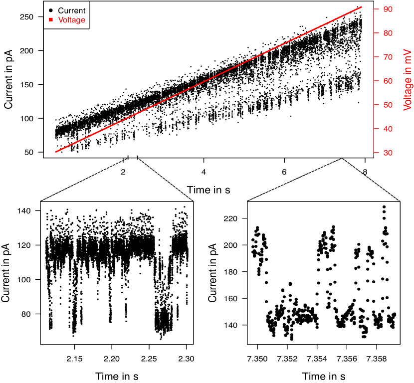
Figure 1. Above: Measurements at a large time scale (seconds) of the current flow of a PorB mutant protein driven by linear increasing voltage from $30mV$-$120mV$.Below: Zoom into finer time scales (decisecond to millisecond).

Figure 2. Conductivity of the protein PorB. The variance of the data decreases in time to a constant.

This is now a sequence $(Z_{n})_{n\in\mathbb{N}}$ of an inhomogeneous HMM. The state of the Markov chain determines the parameter $(\mu^{(1)},\sigma^{(1)})$ or $(\mu^{(2)},\sigma^{(2)})$, both unknown. The non-observable sequence of random variables $(Y_{n})_{n\in\mathbb{N}}$ of the homogeneous HMM is given by

(2) $$Y_{n} :=\mu^{(X_{n})}+\sigma^{(X_{n})}V_{n}.$$

The observation $(Z_{n})_{n\in\mathbb{N}}$ of the inhomogeneous HMM is determined by

(3) $$Z_{n}:=Y_{n}+\varepsilon_{n},$$

with $\varepsilon_{n}=\tilde{\varepsilon}_{n}/u_{n}$, such that $\varepsilon_{n}\sim\mathcal{N}(0,\beta_{n}^{2})$ where $\beta_{n}=\kappa/u_{n}$ and $\lim_{n\to\infty}\beta_{n}^{2}=0,$ as the voltage increases. Such a DHMM describes approximately the observed conductance level of ion channel recordings with linearly increasing voltage.

Intuitively, here one can already see that for sufficiently large $n$ the influence of $\varepsilon_{n}$ “washes out” as $\beta_{n}$ decreases to zero and observations of $Z_{n}$ are “close” to $Y_{n}$.

Main result. We explain now our main theoretical contribution for such a DHMM. Assume that we have a parametrized DHMM $(X_{n},Y_{n},Z_{n})_{n\in\mathbb{N}}$ with compact parameter space $\Theta\subseteq\mathbb{R}^{d}$. For $\theta\in\Theta$ let $q_{\theta}^{\nu}$ be the likelihood function of $Y_{1},\ldots,Y_{n}$ and $p_{\theta}^{\nu}$ be the likelihood function of $Z_{1},\ldots,Z_{n}$ with $X_{0}\sim\nu$. Both functions are assumed to be continuous in $\theta$. Given observations $z_{1},\dots,z_{n}$ of $Z_{1},\dots,Z_{n}$ our goal is to estimate “the true” parameter $\theta^{*}\in\Theta$. The MLE $\theta_{\nu,n}^{\rm\,ML}$, given by a parameter in the set of maximizers of the log-likelihood function, i.e.,

$$\theta_{\nu,n}^{\rm\,ML}\in\arg\!\max_{\theta\in\Theta}\log p_{\theta}^{\nu}(z_{1},\dots,z_{n}),$$

is the canonical estimator for approaching this problem. Note that this set is non-empty due to the compactness of the parameter space and the continuity of $p^{\nu}_{\theta}(z_{1},\ldots,z_{n})$ in $\theta$. Unfortunately none of the strong consistency results of maximum likelihood parameter estimation provided for homogeneous HMMs are applicable, because of the inhomogenity. Namely, all proofs for consistency in HMMs rely on the fact that the conditional distribution of $Z_{n}$ given $X_{n}=x$ is constant for all $n\in\mathbb{N}$. In a DHMM this is usually not the case for $(Z_{n})_{n\in\mathbb{N}}$, because of the time-dependent noise. This issue can be circumvented by proving that under suitable assumptions $(Z_{n})_{n\in\mathbb{N}}$ is an asymptotic mean stationary process. This implies ergodicity and an ergodic theorem for $(Z_{n})_{n\in\mathbb{N}}$, that can be used. However, for the computation of $\theta_{\nu,n}^{\rm\,ML}$ explicit knowledge of the inhomogeneity is needed, i.e., of the time-dependent component of the noise which is hardly known in practice (recall our data example). That is the reason for us to introduce a quasi-maximum likelihood estimator (QMLE), given by a maximizer of the quasi-likelihood function, i.e.,

$$\theta_{\nu,n}^{\rm\,QML}\in\arg\!\max_{\theta\in\Theta}\log q_{\theta}^{\nu}(z_{1},\dots,z_{n}).$$

This is not a MLE, since the observations are generated from the inhomogeneous model, whereas $q_{\theta}^{\nu}$ is the likelihood function of the homogeneous model. Roughly, we assume the following (for a precise definition see Section 3.1):

1. The transition matrix of the hidden finite state space Markov chain is irreducible and satisfies a continuity condition w.r.t. the parameters.

2. The observable and non-observable random variables $(Z_{n})_{n\in\mathbb{N}}$ and $(Y_{n})_{n\in\mathbb{N}}$ are “close” to each other in a suitable sense.

3. The homogeneous HMM is well behaving, such that observations of $(Y_{n})_{n\in\mathbb{N}}$ would lead to a consistent MLE.

We show that if the $Z_{n}$ approximate the $Y_{n}$ reasonably well (see the condition (C1) in Section 3.1 ) the estimator $\theta_{\nu,n}^{\rm\,QML}$ provides also a reasonable way for approximating “the true” parameter $\theta^{*}$. If the model satisfies all conditions, see Section 3.1, then Theorem 1, states that

$$\theta_{\nu,n}^{\rm\,QML}\to\theta^{*}\quad\text{a.s.},\text{ as }n\to\infty.$$

Hence the QMLE is consistent. As a consequence we obtain under an additional assumption that also the MLE is consistent, $\theta_{\nu,n}^{\rm\,ML}\to\theta^{*}$ almost surely, as $n\to\infty$. For a Poisson model and linear Gaussian model we specify Theorem 1, see Section 4. In the DHMM described in (2) and (3) we obtain consistency of the QMLE whenever $\beta_{n}=\mathcal{O}(n^{-q})$ for some $q>0$. In Section 5 we reconsider the approximating condition 2.), precisely stated in Section 3.1, provide an outlook to possible extensions and discuss asymptotic normality of the estimators.

Literature review and connection to our work. The study of maximum likelihood estimation in homogeneous hidden Markov models has a long history and was initiated by Baum and Petrie, see [9, 10], who proved strong consistency of the MLE for finite state spaces $S$ and $G$. Leroux extends this result to general observation spaces in [12]. These consistency results rely on ergodic theory for stationary processes which is not applicable in our setting since the process we observe is not stationary. More precisely, it was shown that the relative entropy rate converges for any parameter $\theta$ in the parameter space $\Theta$ using an ergodic theorem for subadditive processes. There are further extensions also to Markov chains on general state spaces, but under stronger assumptions, see [13, 14, 15, 16, 17]. A breakthrough has been achieved by Douc et al. [11] who used the concept of exponential separability. This strategy allows one to bound the relative entropy rate directly.

Although the state space of the Markov chain is more general than in our setting, we cannot apply the results of [11] due to the inhomogeneity of the observation, but we use the same approach to show our consistency statements.

The investigation of strong consistency of maximum likelihood estimation in inhomogeneous HMMs is less developed. In [18] and [19] the MLE in inhomogeneous Markov switching models is studied. There, the transition probabilities are also influenced by the observations, but the inhomogeneity there is different from the time-dependent inhomogeneity considered in our work, since the conditional law is not changing over time.

Related to strong consistency, as considered here, is the investigation of asymptotic normality (as it provides weak consistency). For homogeneous HMMs asymptotic normality has be shown for example in [14, 20]. In [19], also, asymptotic normality for the MLE in Markov switching models is studied whereas in [21] asymptotic normality of M-estimators in more general inhomogeneous situations is considered. However, the QMLE we suggest and analyze does not satisfy the assumptions imposed there. In Section 5.4 and in Appendix B we provide and discuss necessary conditions to achieve asymptotic normality for the QMLE by adapting the approach of [21].

To ease readability Section 6 is devoted to the proofs of our main results. In particular, we draw the connection between asymptotic mean stationary processes and inhomogeneous hidden Markov models.

2. Setup and notation

We denote the finite state space of $(X_{n})_{n\in\mathbb{N}}$ by $S=\{1,\dots,K\}$ and $\mathcal{S}$ denotes the power set of $S$. Furthermore, let $(G,m)$ be a Polish space with metric $m$ and corresponding Borel $\sigma$-field $\mathcal{B}(G)$. The measurable space $(G,\mathcal{B}(G))$ is equipped with a $\sigma$-finite reference measure $\lambda$. Througout the whole work we consider parametrized families of DHMMs (see Definition 1) with compact parameter space $\Theta\subset\mathbb{R}^{d}$ for some $d\in\mathbb{N}$. For this let $(\mathbb{P}_{\theta})_{\theta\in\Theta}$ be a sequence of probability measures on a measurable space $(\Omega,\mathcal{F})$ such that for each parameter $\theta$ the distribution of $(X_{n},Y_{n},Z_{n})\colon(\Omega,\mathcal{F},\mathbb{P}_{\theta})\to S\times G\times G$ is specified by

• an initial distribution $\nu$ on $S$ and a $K\times K$ transition matrix $P_{\theta}=(P_{\theta}(s,t))_{s,t\in S}$ of the Markov chain $(X_{n})_{n\in\mathbb{N}}$, such that

  $$\mathbb{P}_{\theta}(X_{n}=s)=\nu P_{\theta}^{n-1}(s),\quad s\in S,$$

  where $\nu P_{\theta}^{0}=\nu$ and for $n>1$,

  $$\nu P_{\theta}^{n-1}(s)=\sum_{s_{1},\dots,s_{n-1}\in S}P_{\theta}(s_{n-1},s)\prod_{i=1}^{n-2}P_{\theta}(s_{i},s_{i+1})\nu(s_{1}),\quad s\in S;$$

  (Here and elsewhere we use the convention that $\prod_{i=1}^{0}a_{i}=1$ for any sequence $(a_{i})_{i\in\mathbb{N}}\subset\mathbb{R}$.)

• and by the conditional distribution $Q_{\theta,n}$ of $(Y_{n},Z_{n})$ given $X_{n}=s$, that is,

  $$\mathbb{P}_{\theta}((Y_{n},Z_{n})\in C\mid X_{n}=s)=Q_{\theta,n}(s,C),\qquad C\in\mathcal{B}(G^{2})$$

  which satisfies that there are conditional density functions $f_{\theta},f_{\theta,n}\colon S\times G\to[0,\infty)$ w.r.t. $\lambda$, such that

  $$\mathbb{P}_{\theta}(Y_{n}\in A\mid X_{n}=s) =Q_{\theta,n}(s,A\times G)=\int_{A}f_{\theta}(s,y)\lambda({\rm d}y),\quad A\in\mathcal{B}(G),$$

  $$\mathbb{P}_{\theta}(Z_{n}\in B\mid X_{n}=s) =Q_{\theta,n}(s,G\times B)=\int_{B}f_{\theta,n}(s,z)\lambda({\rm d}z),\;B\in\mathcal{B}(G).$$

  Here the distribution of $Y_{n}$ given $X_{n}=s$ is independent of $n$, whereas the distribution of $Z_{n}$ given $X_{n}=s$ depends through $f_{\theta,n}$ also explicitly on $n$.

By $\mathcal{P}(S)$ we denote the set of probability measures on $S$. To indicate the dependence on the initial distribution, say $\nu\in\mathcal{P}(S)$, we write $\mathbb{P}_{\theta}^{\nu}$ instead of just $\mathbb{P}_{\theta}$. To shorten the notation, let $X=(X_{n})_{n\in\mathbb{N}}$, $Y=(Y_{n})_{n\in\mathbb{N}}$ and $Z=(Z_{n})_{n\in\mathbb{N}}$. Further, let $\mathbb{P}^{\nu,Y}_{\theta}$ and $\mathbb{P}^{\nu,Z}_{\theta}$ be the distributions of $Y$ and $Z$ on $(G^{\mathbb{N}},\mathcal{B}(G^{\mathbb{N}}))$, respectively.

The “true” underlying model parameter will be denoted as $\theta^{*}\in\Theta$ and we assume that the transition matrix $P_{\theta^{*}}$ possesses a unique invariant distribution $\pi\in\mathcal{P}(S)$. We have access to a finite length observation of $Z$. Then, the problem is to find a consistent estimate of $\theta^{*}$ on the basis of the observations without observing $(X_{n},Y_{n})_{n\in\mathbb{N}}$. Consistency of the estimator of $\theta^{*}$ is limited up to equivalence classes in the following sense. Two parameters $\theta_{1},\theta_{2}\in\Theta$ are equivalent, written as $\theta_{1}\sim\theta_{2}$, iff there exist two stationary distributions $\mu_{1},\mu_{2}\in\mathcal{P}(S)$ for $P_{\theta_{1}},P_{\theta_{2}}$, respectively, such that $\mathbb{P}^{\mu_{1},Y}_{\theta_{1}}=\mathbb{P}^{\mu_{2},Y}_{\theta_{2}}$. For the rest of the work assume that each $\theta\in\Theta$ represents its equivalence class.

For an arbitrary finite measure $\nu$ on $(S,\mathcal{S})$, $t\in\mathbb{N}$, $x_{t+1}\in S$ and $z_{1},\ldots,z_{t}\in G$ define

$$p^{\nu}_{\theta}(x_{t+1};z_{1},\ldots,z_{t}) \coloneqq\sum\limits_{x_{1},\ldots,x_{t}\in S}\nu(x_{1})\prod\limits_{i=1}^{t}f_{\theta,i}(x_{i},z_{i})P_{\theta}(x_{i},x_{i+1}),$$

$$p^{\nu}_{\theta}(z_{1},\ldots,z_{t}) \coloneqq\sum\limits_{x_{t+1}\in S}p^{\nu}_{\theta}(x_{t+1};z_{1},\ldots,z_{t}).$$

If $\nu$ is a probability measure on $(S,\mathcal{S})$, then $p^{\nu}_{\theta}(z_{1},\ldots,z_{n})$ is the likelihood of the observations $(Z_{1},\ldots,Z_{n})=(z_{1},\dots,z_{n})\in G^{n}$ for the inhomogeneous HMM $(X_{n},Z_{n})_{n\in\mathbb{N}}$ with parameter $\theta\in\Theta$ and $X_{1}\sim\nu$. Although there are no observations of $Y$ available, we define similar quantities for $(Y_{1},\dots,Y_{n})=(y_{1},\dots,y_{n})\in G^{n}$ by

$$q^{\nu}_{\theta}(x_{t+1},y_{1},\ldots,y_{t}) \coloneqq\sum\limits_{x_{1},\ldots,x_{t}\in S}\nu(x_{1})\prod\limits_{i=1}^{t}f_{\theta}(x_{i},y_{i})P_{\theta}(x_{i},x_{i+1}),$$

$$q^{\nu}_{\theta}(y_{1},\ldots,y_{t}) \coloneqq\sum\limits_{x_{t+1}\in S}q^{\nu}_{\theta}(x_{t+1},y_{1},\ldots,y_{t}).$$

3. Assumptions and main result

Assume for a moment that observations $y_{1},\dots,y_{n}$ of $Y_{1},\dots,Y_{n}$ are available. Then the log-likelihood function of $q_{\theta}^{\nu}$, with initial distribution $\nu\in\mathcal{P}(S)$, is given by

$$\log q_{\theta}^{\nu}(y_{1},\dots,y_{n}).$$

In our setting we do not have access to observations of $Y$, but have access to “contaminated” observations $z_{1},\dots,z_{n}$ of $Z_{1},\dots,Z_{n}$. Based on these observations define a quasi-log-likelihood function

$$\ell^{\,\rm Q}_{\nu,n}(\theta):=\log q_{\theta}^{\nu}(z_{1},\dots,z_{n}),$$

i.e., we plug the contaminated observations into the likelihood of $Y_{1},\ldots,Y_{n}$. Now we approximate $\theta^{*}$ by $\theta_{\nu,n}^{\,\rm QML}$ which is the QMLE, that is,

(4) $$\theta_{\nu,n}^{\,\rm QML}\in\arg\!\max_{\theta\in\Theta}\ell_{\nu,n}^{\,\rm Q}(\theta).$$

In addition, we are interested in the “true” MLE of a realization $z_{1},\ldots,z_{n}$ of $Z_{1},\ldots,Z_{n}$. For this define the log-likelihood function

$$\ell_{\nu,n}(\theta):=\log p_{\theta}^{\nu}(z_{1},\dots,z_{n}),$$

which leads to the MLE $\theta_{\nu,n}^{\,\rm ML}$ given by

(5) $$\theta_{\nu,n}^{\,\rm ML}\in\arg\!\max_{\theta\in\Theta}\ell_{\nu,n}(\theta).$$

Under certain structural assumptions we prove that the QMLE from (4) is consistent. By adding one more condition this result can be used to verify that the MLE from (5) is also consistent.

3.1. Structural conditions

We prove consistency of the QMLE $\theta_{\nu,n}^{\rm\,QML}$ and the MLE $\theta_{\nu,n}^{\,\rm ML}$ under the following structural assumptions:

Irreducibility and continuity of $X$

1. The transition matrix $P_{\theta^{*}}$ is irreducible.

2. The parametrization $\theta\mapsto P_{\theta}$ is continuous.

Proximity of $Y$ and $Z$

1. There exists $p>1$ such that for any $s\in S$ and $\varepsilon>0$ we have

   $$\mathbb{P}_{\theta^{*}}\left(m(Z_{n},Y_{n})\geq\varepsilon\mid X_{n}=s\right)=\mathcal{O}(n^{-p}).$$

   (Recall that $m$ is the metric on $G$.)

2. There exists an integer $k\in\mathbb{N}$ such that

   (6) $$\mathbb{P}_{\theta^{*}}^{\pi}\left(\prod_{i=1}^{k-1}\max_{s\in S}\frac{f_{\theta^{*},i}(s,Z_{i})}{f_{\theta^{*}}(s,Z_{i})}<\infty\right) =1,$$

   $$\mathbb{E}_{\theta^{*}}^{\pi}\left[\max\limits_{s^{\prime}\in S}\frac{f_{\theta^{*},n}(s^{\prime},Z_{n})}{f_{\theta^{*}}(s^{\prime},Z_{n})}\mid X_{n}=s\right] <\infty,\quad\forall s\in S,n\geq k,$$

   and

   (7) $$\limsup\limits_{n\rightarrow\infty}\mathbb{E}_{\theta^{*}}^{\pi}\left[\max\limits_{s^{\prime}\in S}\frac{f_{\theta^{*},n}(s^{\prime},Z_{n})}{f_{\theta^{*}}(s^{\prime},Z_{n})}\mid X_{n}=s\right]\leq 1,\quad\forall s\in S.$$

3. For every $\theta\in\Theta$ with $\theta\not\sim\theta^{*}$, there exists a neighborhood $\mathcal{E}_{\theta}$ of $\theta$ such that there exists an integer $k\in\mathbb{N}$ with

   (8) $$\mathbb{P}_{\theta^{*}}^{\pi}\left(\prod_{i=1}^{k-1}\sup\limits_{\theta^{\prime}\in\mathcal{E}_{\theta}}\max_{s\in S}\frac{f_{\theta^{\prime},i}(s,Z_{i})}{f_{\theta^{\prime}}(s,Z_{i})}<\infty\right) =1,$$

   $$\mathbb{E}_{\theta^{*}}^{\pi}\left[\sup\limits_{\theta^{\prime}\in\mathcal{E}_{\theta}}\max\limits_{s^{\prime}\in S}\frac{f_{\theta^{\prime},n}(s^{\prime},Z_{n})}{f_{\theta^{\prime}}(s^{\prime},Z_{n})}\mid X_{n}=s\right] <\infty,\quad\forall s\in S,n\geq k,$$

   and

   (9) $$\lim\limits_{n\rightarrow\infty}\left(\mathbb{E}_{\theta^{*}}^{\pi}\left[\sup\limits_{\theta^{\prime}\in\mathcal{E}_{\theta}}\max\limits_{s^{\prime}\in S}\frac{f_{\theta^{\prime},n}(s^{\prime},Z_{n})}{f_{\theta^{\prime}}(s^{\prime},Z_{n})}\mid X_{n}=s\right]\right)=1,\quad\forall s\in S.$$

Remark 1.

(C1) guarantees in particular that $m(Z_{n},Y_{n})$ converges $\mathbb{P}_{\theta*}$-a.s. to zero whereas (C2) ensures that the ratio of $p^{\nu}_{\theta^{*}}(z_{1},\ldots,z_{n})$ and $q^{\nu}_{\theta^{*}}(z_{1},\ldots,z_{n})$ does not diverge exponentially or faster. Assumption (C3) is needed to carry over the consistency of the QMLE to the MLE. In particular it implies that for all $\theta\not\sim\theta^{*}$ the ratio of $p^{\nu}_{\theta}(z_{1},\ldots,z_{n})$ and $q^{\nu}_{\theta}(z_{1},\ldots,z_{n})$ does not diverge exponentially or faster uniformly in $\mathcal{E}_{\theta}$.

Well behaving HMM

It is plausible that we are only able to prove consistency in the case where the unobservable sequence $Y$ would lead to a consistent estimator of $\theta^{*}$, itself. To guarantee that this is indeed the case we assume:

1. For all $s\in S$ let $\mathbb{E}^{\pi}_{\theta^{*}}\left[\left|\log f_{\theta^{*}}(s,Y_{1})\right|\right]<\infty$.

2. For every $\theta\in\Theta$ with $\theta\not\sim\theta^{*}$, there exists a neighborhood $\mathcal{U}_{\theta}$ of $\theta$ such that

   $$\mathbb{E}^{\pi}_{\theta^{*}}\left[\sup\limits_{\theta^{\prime}\in\mathcal{U}_{\theta}}(\log f_{\theta^{\prime}}(s,Y_{1}))^{+}\right]<\infty\qquad\text{ for all }s\in S.$$

3. The mappings $\theta\mapsto f_{\theta}(s,y)$ and $\theta\mapsto f_{\theta,n}(s,y)$ are continuous for any $s\in S$, $n\in\mathbb{N}$ and $y\in G$.

4. For all $s\in S$ and $n\in\mathbb{N}$ let $\mathbb{E}^{\pi}_{\theta^{*}}\left[\left|\log f_{\theta^{*},n}(s,Z_{n})\right|\right]<\infty$.

Remark 2.

The conditions (H1)–(H3) coincide with the assumptions in [11, Sect. 3.2.] for finite state models and guarantee that the MLE for $\theta^{*}$ based on observations of $Y$ is consistent. The condition (H4) is an additional regularity assumption required for the inhomogeneous setting.

3.2. Consistency theorem

Now we formulate our main results about the consistency of the QMLE and the MLE.

Theorem 1.

Assume that the irreducibility and continuity conditions (P1), (P2), the proximity conditions (C1), (C2) and the well behaving HMM conditions (H1)–(H4) are satisfied. Further, let the initial distribution $\nu\in\mathcal{P}(S)$ be strictly positive if and only if $\pi$ is strictly positive. Then

$$\theta^{\,\rm QML}_{\nu,n}\rightarrow\theta^{*},\quad\mathbb{P}_{\theta^{*}}^{\pi}\text{-a.s.}$$

as $n\rightarrow\infty$.

Note that condition (C3) is not required in the previous statement. We only need it to prove the consistency of the MLE $\theta^{\rm\,ML}_{\nu,n}$.

Corollary 1.

Assume that the setting and conditions of Theorem 1 and (C3) are satisfied. Then

$$\theta^{\rm\,ML}_{\nu,n}\rightarrow\theta^{*},\quad\mathbb{P}_{\theta^{*}}^{\pi}\text{-a.s.}$$

as $n\rightarrow\infty$.

4. Application

We consider two models where we explore the structural assumptions from Section 3.1 explicitly. The Poisson model, see Section 4.1, illustrates a simple example with countable observation space. The linear Gaussian model is an extension of the model introduced in (1) and (2) to multivariate and possibly correlated observations.

4.1. Poisson DHMM

For $i=1,\dots,K$ let $\lambda_{\theta^{*}}^{(i)}>0$ and define the vector $\lambda_{\theta^{*}}=(\lambda_{\theta^{*}}^{(1)},\ldots,\lambda_{\theta^{*}}^{(K)})$. Conditioned on $X$ the non-observed homogeneous sequence $Y=(Y_{n})_{n\in\mathbb{N}}$ is an independent sequence of Poisson-distributed random variables with parameter $\lambda_{\theta^{*}}^{(X_{n})}$. In other words, given $X_{n}=x_{n}$ we have $Y_{n}\sim\text{Poi}(\lambda_{\theta^{*}}^{(x_{n})})$. Here $\text{Poi}(\alpha)$ denotes the Poisson distribution with expectation $\alpha>0$. The observed sequence $Z=(Z_{n})_{n\in\mathbb{N}}$ is determined by

$$Z_{n}=Y_{n}+\varepsilon_{n},$$

where $(\varepsilon_{n})_{n\in\mathbb{N}}$ is an independent sequence of random variables with $\varepsilon_{n}\sim\text{Poi}(\beta_{n})$. Here $(\beta_{n})_{n\in\mathbb{N}}$ is a sequence of positive real numbers satisfying for some $p>1$ that

(10) $$\beta_{n}=\mathcal{O}(n^{-p}).$$

We also assume that $(\varepsilon_{n})_{n\in\mathbb{N}}$ is independent of $Y$ and that the parameter $\theta$ determines the transition matrix $P_{\theta}$ and the intensity $\lambda_{\theta}$ continuously. Note that the observation space is given by $G=\mathbb{N}\cup\{0\}$ equipped with the counting measure $\lambda$. Figures 3 illustrates the empirical mean square error of approximations of the MLEs.

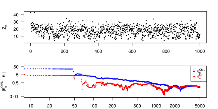
Figure 3. Exemplary trajectory of observations of the Poisson model from Section 4.1 (above) and Euclidean norm of the difference of $\theta^{*}$ and the estimators based on a single trajectory of observations (below). Here $K=2$, $n=5\cdot 10^{3}$ and $\theta^{*}=(10,20,0.8,0.1)$. The parameter $\theta^{*}$ determines $\lambda_{\theta^{*}}=(10,20)$ and the “true” transition matrix by $P_{\theta^{*}}(1,1)=0.8$, $P_{\theta^{*}}(2,1)=0.1$. The inhomogeneous noise is driven by an intensity $\beta_{n}=40\,n^{-1.01}$.

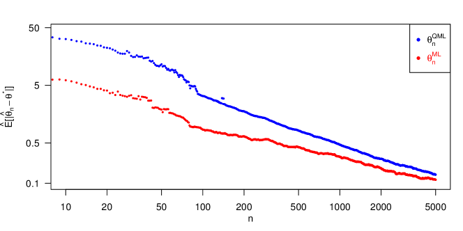
Figure 4. Empirical mean of the Euclidean norm of the difference of $\theta^{*}$ and the estimators based on $100$ i.i.d. replications of the DHMM. Here $K=2$, $n=5\cdot 10^{3}$ and $\theta^{*}=(10,20,0.8,0.1)$. The parameter $\theta^{*}$ determines $\lambda_{\theta^{*}}=(10,20)$ and the “true” transition matrix by $P_{\theta^{*}}(1,1)=0.8$, $P_{\theta^{*}}(2,1)=0.1$. The inhomogeneous noise is driven by an intensity $\beta_{n}=40\,n^{-1.01}$.

To obtain the desired consistency of the two estimators we need to check the conditions (P1), (P2), (C1)–(C3) and (H1)–(H4):

To (P1) and (P2): By the assumptions in this scenario those conditions are satisfied.

To (H1)–(H4): For $\theta\in\Theta$, $s\in S$ and $y\in G$ we have

$$\left|\log f_{\theta}(s,y)\right|=-\log\left(\frac{\left(\lambda_{\theta}^{(s)}\right)^{y}}{y!}\exp(-\lambda_{\theta}^{(s)})\right) =-y\log(\lambda_{\theta}^{(s)})+\log(y!)+\lambda_{\theta}^{(s)}$$

$$\leq-y\log(\lambda_{\theta}^{(s)})+y^{2}+\lambda_{\theta}^{(s)}.$$

Hence

$$\mathbb{E}_{\theta^{*}}^{\pi}\left[\left|\log f_{\theta^{*}}(s,Y_{1})\right|\right]$$

$$\leq-\log(\lambda_{\theta^{*}}^{(s)})\sum_{s=1}^{K}\pi(s)\lambda_{\theta^{*}}^{(s)}+\sum_{s=1}^{K}\pi(s)\left(\left(\lambda_{\theta^{*}}^{(s)}\right)^{2}+\lambda_{\theta^{*}}^{(s)}\right)+\lambda_{\theta^{*}}^{(s)}<\infty$$

and (H1) is verified. A similar calculation gives (H4). Condition (H2) follows simply by $(\log f_{\theta}(s,y))^{+}=0$. Condition (H3) follows by the continuity in the parameter of the probability function of the Poisson distribution and the continuity of the mapping $\theta\mapsto(P_{\theta},\lambda_{\theta})$.

To (C1) – (C3): For any $\delta>0$ and any $s\in S$ we have

$$\mathbb{P}_{\theta}^{\pi}\left(\left|Z_{n}-Y_{n}\right|\geq\delta\mid X_{n}=s\right)=\mathbb{P}_{\theta}^{\pi}\left(\left|\varepsilon_{n}\right|\geq\delta\right)\leq 1-\mathbb{P}_{\theta}^{\pi}\left(\varepsilon_{n}=0\right)=1-\exp(-\beta_{n}).$$

From (10) it follows that

$$1-\exp(-\beta_{n})=\mathcal{O}(n^{-p}),$$

which proves (C1). Observe that for any $s\in S,z\in G$ we have

$$\max\limits_{s\in S}\frac{f_{\theta^{*},n}(s,z)}{f_{\theta^{*}}(s,z)}=\max\limits_{s\in S}\frac{\left(\beta_{n}+\lambda_{\theta^{*}}^{(s)}\right)^{z}}{\left(\lambda_{\theta^{*}}^{(s)}\right)^{z}}\exp(-\beta_{n})=\left(a_{n}\right)^{z}\exp(-\beta_{n}),$$

with $a_{n}=\max\limits_{s\in S}\frac{\beta_{n}+\lambda_{\theta^{*}}^{(s)}}{\lambda_{\theta^{*}}^{(s)}}$. Now we verify (C2) with $k=1$. For all $n\in\mathbb{N}$ and $s\in S$ we have

$$\mathbb{E}_{\theta^{*}}^{\pi}\left[\max\limits_{s^{\prime}\in S}\frac{f_{\theta^{*},n}(s^{\prime},Z_{n})}{f_{\theta^{*}}(s^{\prime},Z_{n})}\mid X_{n}=s\right] =\mathbb{E}_{\theta^{*}}^{\pi}\left[a_{n}^{Z_{n}}\exp(-\beta_{n})\mid X_{n}=s\right]$$

$$=\exp\left((\lambda_{\theta^{*}}^{(s)}+\beta_{n})(a_{n}-1)-\beta_{n}\right)<\infty.$$

Fix $s\in S$, and note that

$$\limsup\limits_{n\rightarrow\infty}\mathbb{E}_{\theta^{*}}^{\pi}\left[\max\limits_{s^{\prime}\in S}\frac{f_{\theta^{*},n}(s^{\prime},Z_{n})}{f_{\theta^{*}}(s^{\prime},Z_{n})}\mid X_{n}=s\right]$$

$$=\limsup\limits_{n\rightarrow\infty}\exp\left((\lambda_{\theta^{*}}^{(s)}+\beta_{n})(a_{n}-1)-\beta_{n}\right)=1.$$

The last equality follows by the fact that $\lim_{n\to\infty}a_{n}=1$ and $\lim_{n\to\infty}\beta_{n}=0$. Condition (C3) follows by similar arguments.

The application of Theorem 1 and Corollary 1 leads to the following result.

Corollary 2.

For any initial distribution $\nu\in\mathcal{P}(S)$ which is strictly positive if and only if $\pi$ is strictly positive, we have for the Poisson DHMM if (10) holds for some $p>1$ that

$$\theta^{\,\rm QML}_{\nu,n}\rightarrow\theta^{*},\quad\mathbb{P}_{\theta^{*}}^{\pi}\text{-a.s.}$$

and

$$\theta^{\,\rm ML}_{\nu,n}\rightarrow\theta^{*},\quad\mathbb{P}_{\theta^{*}}^{\pi}\text{-a.s.}$$

as $n\rightarrow\infty$.

4.2. Multivariate linear Gaussian DHMM

For $i=1,\dots,K$ let $\mu_{\theta^{*}}^{(i)}\in\mathbb{R}^{M}$, $\Sigma_{\theta^{*}}^{(i)}\in\mathbb{R}^{M\times M}$ with full rank, where $M\in\mathbb{N}$. Define $\mu_{\theta^{*}}=(\mu_{\theta^{*}}^{(1)},\ldots,\mu_{\theta^{*}}^{(K)})$ as well as $\Sigma_{\theta^{*}}=(\Sigma_{\theta^{*}}^{(1)},\ldots,\Sigma_{\theta^{*}}^{(K)}).$ The sequences $Y=(Y_{n})_{n\in\mathbb{N}}$ and $Z=(Z_{n})_{n\in\mathbb{N}}$ are defined by

$$Y_{n} =\mu_{\theta^{*}}^{(X_{n})}+\Sigma_{\theta^{*}}^{(X_{n})}V_{n}$$

$$Z_{n} =Y_{n}+\varepsilon_{n}.$$

Here $(V_{n})_{n\in\mathbb{N}}$ is an i.i.d. sequence of random vectors with $V_{n}\sim\mathcal{N}(0,I)$, where $I\in\mathbb{R}^{M\times M}$ denotes the identity matrix, and $(\varepsilon_{n})_{n\in\mathbb{N}}$ is a sequence of independent random vectors with $\varepsilon_{n}\sim\mathcal{N}(0,\beta_{n}^{2}I)$, where $(\beta_{n})_{n\in\mathbb{N}}$ is a positive real-valued sequence satisfying for some $q>0$ that

(11) $$\beta_{n}=\mathcal{O}(n^{-q}).$$

Here we also assume that the mapping $\theta\mapsto(P_{\theta},\mu_{\theta},\Sigma_{\theta})$ is continuous. Furthermore, note that $G=\mathbb{R}^{M}$ and $\lambda$ is the $M$-dimensional Lebesgue measure. Figures 5 illustrates the empirical mean square error of approximations of the MLEs.

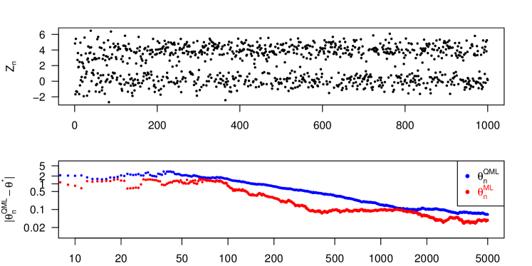
Figure 5. Exemplary trajectory of observations of the linear Gaussian model from Section 4.2 (above) and Euclidean norm of the difference of $\theta^{*}$ and the estimators based on a single trajectory of observations (below). Here $M=1$, $K=2$, $n=5\cdot 10^{3}$ and $\theta^{*}=(0,4,0.5,0.5,0.4,0.5)$. The parameter $\theta^{*}$ determines $\mu_{\theta^{*}}=(0,4)$, $\Sigma_{\theta^{*}}=(0.5,0.5)$ and the “true” transition matrix by $P_{\theta^{*}}(1,1)=0.4$, $P_{\theta^{*}}(2,1)=0.5$. The inhomogeneous noise is driven by an intensity $\beta_{n}=10\,n^{-0.75}$.

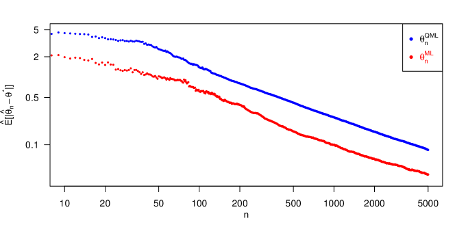
Figure 6. Empirical mean of the Euclidean norm of the difference of $\theta^{*}$ and the estimators norm based on $100$ i.i.d. replications of the DHMM. Here $M=1$, $K=2$, $n=5\cdot 10^{3}$ and $\theta^{*}=(0,4,0.5,0.5,0.4,0.5)$. The parameter $\theta^{*}$ determines $\mu_{\theta^{*}}=(0,4)$, $\Sigma_{\theta^{*}}=(0.5,0.5)$ and the “true” transition matrix by $P_{\theta^{*}}(1,1)=0.4$, $P_{\theta^{*}}(2,1)=0.5$. The inhomogeneous noise is driven by an intensity $\beta_{n}=10\,n^{-0.75}$.

To obtain consistency of the two estimators we need to check the conditions (P1), (P2), (C1)–(C3) and (H1)–(H4):

To (P1) and (P2): By definition of the model this conditions are satisfied.

To (H1)–(H4): For a matrix $A\in\mathbb{R}^{M\times M}$ denote $A^{2}=AA^{T}$ and $A^{-2}=(A^{2})^{-1}$. Note that for $s\in S$, $\theta\in\Theta$ and $y,z\in G$ we have by

$$f_{\theta}(s,y) =\frac{(2\pi)^{-M/2}}{\det\left(\left(\Sigma_{\theta}^{(s)}\right)^{2}\right)^{1/2}}\exp\left(-\frac{1}{2}(y-\mu_{\theta}^{(s)})^{T}\left(\Sigma_{\theta}^{(s)}\right)^{-2}(y-\mu_{\theta}^{(s)})\right),$$

$$f_{\theta,n}(s,z) =\frac{(2\pi)^{-M/2}}{\det\left(\left(\Sigma_{\theta}^{(s)}\right)^{2}+\beta_{n}^{2}I\right)^{1/2}}$$

$$\qquad\qquad\qquad\times\exp\left(-\frac{1}{2}(z-\mu_{\theta}^{(s)})^{T}\left(\left(\Sigma_{\theta}^{(s)}\right)^{2}+\beta_{n}^{2}I\right)^{-1}(z-\mu_{\theta}^{(s)})\right).$$

Further, observe that $\det\left(\left(\Sigma_{\theta}^{(s)}\right)^{2}\right)>0$ for all $s\in S$. For some constant $C_{1}>0$ we have

$$\mathbb{E}_{\theta^{*}}^{\pi}\left[\left|\log f_{\theta}(s,Y_{1})\right|\right] \leq C_{1}+\mathbb{E}_{\theta^{*}}^{\pi}\left[\frac{1}{2}(Y_{1}-\mu_{\theta}^{(s)})^{T}\left(\Sigma_{\theta}^{(s)}\right)^{-2}(Y_{1}-\mu_{\theta}^{(s)})\right]<\infty,$$

since for each $i,j\in\{1,\dots,M\}$ we have $\mathbb{E}_{\theta^{*}}^{\pi}\left[Y_{1}^{(i)}Y_{1}^{(j)}\right]<\infty$ with the notation $Y_{1}=(Y_{1}^{(1)},\dots,Y_{1}^{(M)})$. By this estimate (H1) and (H2) follows easily. Condition (H4) follows by similar arguments. More detailed, we have that $\beta_{n}^{2}$ is finite and converges to zero as well, as that there exists a constant $C_{2}>0$ such that

$$\mathbb{E}_{\theta^{*}}^{\pi}\left[\left|\log f_{\theta^{*},n}(s,Z_{n})\right|\right] \leq C_{2}+\mathbb{E}_{\theta^{*}}^{\pi}\left[\frac{1}{2}(Z_{n}-\mu_{s})^{T}\left(\left(\Sigma_{\theta}^{(s)}\right)^{2}+\beta_{n}^{2}I\right)^{-1}(Z_{n}-\mu_{s})\right].$$

For all $n\in\mathbb{N}$ the right-hand side of the previous inequality is finite, since for each $i,j\in\{1,\dots,M\}$ we have $\mathbb{E}_{\theta^{*}}^{\pi}\left[Z_{n}^{(i)}Z_{n}^{(j)}\right]<\infty$, with $Z_{n}=(Z_{n}^{(1)},\dots,Z_{n}^{(M)})$. Finally condition (H3) is satisfied by the continuity of the conditional density and the continuity of the mapping $\theta\mapsto(P_{\theta},\mu_{\theta},\Sigma_{\theta})$.

To (C1) – (C3): Here $m$ is the Euclidean metric in $\mathbb{R}^{M}$ such that $\left|\varepsilon_{n}\right|=m(Y_{n},Z_{n})$. Fix some $r>0$ with $r/q>1$ and observe that for any $\delta>0$ and $s\in S$ we have

$$\mathbb{P}_{\theta^{*}}^{\pi}\left(m(Y_{n},Z_{n})>\delta\mid X_{n}=s\right)=\mathbb{P}_{\theta^{*}}^{\pi}\left(\left|\varepsilon_{n}\right|>\delta\right)=\mathbb{P}_{\theta^{*}}^{\pi}\left(\beta_{n}^{r}\left|N\right|^{r}>\delta^{r}\right)\leq\frac{\mathbb{E}_{\theta^{*}}^{\pi}\left[\left|N\right|^{r}\right]\beta_{n}^{r}}{\delta^{r}},$$

where $N\sim\mathcal{N}(0,I)$. By the fact that $\mathbb{E}_{\theta^{*}}^{\pi}\left[\left|N\right|^{r}\right]<\infty$ and (11) we obtain that condition (C1) is satisfied with $p=r/q>1$.

The requirement of (6) of (C2) holds for any $k\in\mathbb{N}$, since the density of normally distributed random vectors is strictly positive and finite. Observe that

$$\max\limits_{s\in S}\frac{f_{\theta,n}(s,Z_{n})}{f_{\theta}(s,Z_{n})}\leq$$

$$\qquad C_{n}\max\limits_{s\in S}\exp\left(-\frac{1}{2}(Z_{n}-\mu_{\theta}^{(s)})^{T}\left(((\Sigma^{(s)}_{\theta})^{2}+\beta_{n}^{2}I)^{-1}-(\Sigma^{(s)}_{\theta})^{-2}\right)(Z_{n}-\mu_{\theta}^{(s)})\right),$$

with

$$C_{n}:=\max\limits_{s\in S}\frac{\left(\det\left(\left(\Sigma_{\theta}^{(s)}\right)^{2}\right)\right)^{1/2}}{\left(\det\left(\left(\Sigma_{\theta}^{(s)}\right)^{2}+\beta_{n}^{2}I\right)\right)^{1/2}}.$$

Note that $\lim_{n\rightarrow\infty}C_{n}=1$. Since for an invertible matrix $A\in\mathbb{R}^{M\times M}$, $A\mapsto A^{-1}$ is continuous and $\Sigma_{\theta^{*}}^{s}$ has full rank, it follows that

$$\lim\limits_{n\rightarrow\infty}\left(\left(\Sigma_{\theta}^{(s)}\right)^{2}+\beta_{n}^{2}I\right)^{-1}=\left(\Sigma_{\theta}^{(s)}\right)^{-2}.$$

f Set $(\Sigma_{\theta}^{(s)})^{2}_{n}:=(\Sigma_{\theta}^{(s)})^{2}+\beta_{n}^{2}I$ and define $B_{n}=B_{n,s}:=(\Sigma_{\theta}^{(s)})^{-2}-(\Sigma_{\theta}^{(s)})_{n}^{-2}$. Note that the entries of $B_{n}$ converge to zero when $n$ goes to infinity.

Further, by the fact that $(B_{n})_{n\in\mathbb{N}}$ is a sequence of symmetric, positive definite matrices there exist sequences of orthogonal matrices $(U_{n})_{n\in\mathbb{N}}\subset\mathbb{R}^{M\times M}$ and diagonal matrices $(D_{n})_{n\in N}\subset\mathbb{R}^{M\times M}$ such that

$$B_{n}=U_{n}^{T}D_{n}^{1/2}D_{n}^{1/2}U_{n}.$$

Of course, $U_{n}$ and $D_{n}$ depend on $s$. We define a sequence of random vectors $(W_{n,s})_{n\in\mathbb{N}}$ by setting $W_{n,s}:=U_{n}D_{n}^{1/2}(Z_{n}-\mu_{\theta}^{(s)})$, such that

$$(Z_{n}-\mu_{\theta}^{(s)})^{T}\left((\Sigma^{(s)}_{\theta})^{-2}-((\Sigma^{(s)}_{\theta})^{2}+\beta_{n}^{2}I)^{-1}\right)(Z_{n}-\mu_{\theta}^{(s)})$$

$$=(Z_{n}-\mu_{\theta}^{(s)})^{T}B_{n}(Z_{n}-\mu_{\theta}^{(s)})=W_{n,s}^{T}W_{n,s}.$$

The random variable $Z_{i}$ conditioned on $X_{i}=x$ is normally distributed with mean $\mu_{\theta}^{(x)}$ and covariance matrix $(\Sigma_{\theta}^{(x)})^{2}_{n}$. Hence $W_{i,s}$, conditioned on $X_{i}=x$, satisfies

$$W_{i,s}\sim\mathcal{N}(\tilde{\mu}_{i},A_{i}),$$

with

$$\tilde{\mu}_{i}=U_{i}^{T}D_{i}^{1/2}(\mu_{\theta}^{(x)}-\mu_{\theta}^{(s)})$$

and

$$A_{i}=U_{i}^{T}D_{i}^{1/2}(\Sigma_{\theta}^{(x)})^{2}_{i}(U_{i}^{T}D_{i}^{1/2})^{T}.$$

Since $A_{i}$ is symmetric and positive definite, we find sequences of orthogonal matrices $(U^{\prime}_{n})_{n\in\mathbb{N}}$ and diagonal matrices $(D_{n}^{\prime})_{n\in\mathbb{N}}$ depending on $x$ and $s$ such that

$$A_{i}=U_{i}^{\prime}D_{i}^{\prime 1/2}D_{i}^{\prime 1/2}U_{i}^{\prime T}.$$

Let $(N_{i})_{i\in\mathbb{N}}$ be an i.i.d. sequence of random vectors with $N_{i}\sim\mathcal{N}(0,I)$ and denote $N_{i}=(N_{i}^{(1)},\dots,N_{i}^{(M)})$. Then

$$W_{i,s}^{T}W_{i,s} =\left|W_{i,s}\right|^{2}\stackrel{{\scriptstyle\mathcal{D}}}{{=}}\left|U_{i}^{\prime}D_{i}^{\prime 1/2}(N_{i}+D_{i}^{\prime-1/2}U_{i}^{\prime T}\tilde{\mu}_{i})\right|^{2}$$

$$=\left|D_{i}^{\prime 1/2}(N_{i}+D_{i}^{\prime-1/2}U_{i}^{\prime T}\tilde{\mu}_{i})\right|^{2}=\sum_{j=1}^{M}D^{\prime}_{i}(j,j)\left(N_{i}^{(j)}+(D_{i}^{\prime-1/2}U_{i}^{\prime T}\tilde{\mu}_{i})^{(j)}\right)^{2}.$$

Recall that for a chi-squared distribution with one degree of freedom and non-centrality parameter $\gamma>0$ the moment generating function in $t$, with $t<1/2$, is given by $\frac{\exp(\gamma t/(1-2t))}{(1-2t)^{1/2}}$. Hence, for any $t<\min_{j=1,\dots,M}D^{\prime}_{i}(j,j)^{-1}$ with non-centrality parameter $(D_{i}^{\prime-1/2}U_{i}^{\prime T}\tilde{\mu}_{i})^{(j)}$ at $\frac{t}{2}D_{i}^{\prime}(j,j)$ it is well-defined and we obtain

$$\mathbb{E}_{\theta^{*}}^{\pi}\left[\exp\left(\frac{t}{2}W_{i,s^{\prime}}^{T}W_{i,s^{\prime}}\right)\mid X_{i}=s\right]$$

$$=\prod\limits_{j=1}^{M}(1-2(\frac{t}{2})D^{\prime}_{i}(j,j))^{-1/2}\exp\left(\frac{(D_{i}^{\prime-1/2}U_{i}^{\prime T}\tilde{\mu}_{i})^{(j)}(\frac{t}{2})D^{\prime}_{i}(j,j)}{1-2(\frac{t}{2})D^{\prime}_{i}(j,j)}\right)$$

$$=\prod\limits_{j=1}^{M}(1-tD^{\prime}_{i}(j,j))^{-1/2}\exp\left(\frac{(D_{i}^{\prime-1/2}U_{i}^{\prime T}\tilde{\mu}_{i})^{(j)}(\frac{t}{2})D^{\prime}_{i}(j,j)}{1-tD^{\prime}_{i}(j,j)}\right)\rightarrow 1$$

as $i\rightarrow\infty$, since $\lim\limits_{i\rightarrow\infty}D_{i}^{\prime}(j,j)=0$ for all $j=1,\dots,M$. We can choose $k$ sufficiently large, such that $K<\min_{j=1,\dots,M}D^{\prime}_{i}(j,j)^{-1}$ for all $i\geq k$. We find that

$$\mathbb{E}_{\theta^{*}}^{\pi} \left[\max\limits_{s^{\prime}\in S}\exp\left(\frac{1}{2}W_{k,s^{\prime}}^{T}W_{k,s^{\prime}}\right)\mid X_{k}=s\right]\leq\mathbb{E}_{\theta^{*}}^{\pi}\left[\sum\limits_{s^{\prime}\in S}\exp\left(\frac{1}{2}W_{k,s^{\prime}}^{T}W_{k,s^{\prime}}\right)\mid X_{k}=s\right]$$

$$\leq\prod\limits_{s^{\prime}\in S}\left(\mathbb{E}_{\theta^{*}}^{\pi}\left[\exp\left(\frac{K}{2}W_{k,s^{\prime}}^{T}W_{k,s^{\prime}}\right)\mid X_{k}=s\right]\right)^{1/K},$$

where we used the generalized Hölder inequality in the last estimate. Then, by taking the limit superior we obtain that the right-hand side of the previous inequality goes to one for $k\to\infty$ such that (C2) holds. Condition (C3) can be verified similarly.

The application of Theorem 1 and Corollary 1 leads to the following result.

Corollary 3.

For any initial distribution $\nu\in\mathcal{P}(S)$ which is strictly positive if and only if $\pi$ is strictly positive, we have for the multivariate Gaussian DHMM satisfying (11) for some $q>0$ that

$$\theta^{\,\rm QML}_{\nu,n}\rightarrow\theta^{*},\quad\mathbb{P}_{\theta^{*}}^{\pi}\text{-a.s.}$$

and

$$\theta^{\,\rm ML}_{\nu,n}\rightarrow\theta^{*},\quad\mathbb{P}_{\theta^{*}}^{\pi}\text{-a.s.}$$

as $n\rightarrow\infty$.

Remark 3.

For $K=2$ and $M=1$ we have the model of the conductance level of ion channel data with varying voltage provided in the introduction, see Figure 1 and (2) and (3). The previous corollary states the desired consistency of the considered MLEs in that setting. A data analysis of the ion channel recordings of the underlying DHMM will be done in a separate paper.

5. Discussion and limitations

In this section we discuss four aspects. First, having the models from Section 4 in mind, one might consider a hybrid case, that is, e.g. if the non-observed sequence $Y$ is Poisson distributed and the inhomogeneous noise is normally distributed. We discuss where our approach fails here and provide a strategy how to resolve this issue. Second, one might ask whether the proximity assumptions formulated in Section 3.1 can be relaxed. We provide a simple example where (C1) is not satisfied and $\theta_{\nu,n}^{\rm QML}$ is not consistent anymore. Third, we discuss the restriction of considering only hidden Markov chains on finite state spaces. Finally, we comment and discuss conditions which lead to asymptotic normality of the QMLE.

5.1. Hybrid model

The hidden sequences $X$ and $Y$ of the DHMM are defined as in Section 4.1. The observed sequence $Z=(Z_{n})_{n\in\mathbb{N}}$ is given by

$$Z_{n}=Y_{n}+\varepsilon_{n},$$

where $(\varepsilon_{n})_{n\in\mathbb{N}}$ is an independent sequence of random variables with $\varepsilon_{n}\sim\mathcal{N}(0,\beta^{2}_{n})$ and a $(\beta_{n})_{n\in\mathbb{N}}\subset(0,\infty)$ satisfies $\lim_{n\to\infty}\beta_{n}^{2}=0$. In other words, on the Poisson random variable $Y_{n}$ we add Gaussian time-dependent noise.

The main issue is that the observed sequence $Z$ takes values in $\mathbb{R}$ whereas $Y$ takes values in $\mathbb{N}\cup\{0\}$. Consider $G=\mathbb{R}$ equipped with the reference measure $\lambda(\cdot)=\mathcal{L}(\cdot)+\sum_{i=0}^{\infty}\delta_{i}(\cdot)$. Here $\mathcal{L}(\cdot)$ denotes the Lebesgue measure and $\delta_{i}(\cdot)$ the Dirac-measure at point $i\in\mathbb{N}$. The conditional density $f_{\theta,n}$ w.r.t. $\lambda$ is given by

$$f_{\theta,n}(s,z)=\begin{cases}\sum_{j=0}^{\infty}\frac{\lambda_{\theta}^{(s)}}{j!}\exp(-\lambda_{\theta}^{(s)})\frac{1}{(2\pi\beta_{n}^{2})^{1/2}}\exp\left(-\frac{(z-j)^{2}}{2\beta_{n}^{2}}\right)&\quad z\in\mathbb{R}\backslash\mathbb{N}\\ 0&\quad z\in\mathbb{N}.\end{cases}$$

One can verify that (C2) is not satisfied in this scenario. In general, assumption (C2) is difficult to handle, whenever the support of $f_{\theta}$ is strictly “smaller” than the support of $f_{\theta,n}$. We mention a possible strategy to resolve this problem:

1. Transform the observed sequence to a sequence $\tilde{Z}=(\widetilde{Z}_{n})_{n\in\mathbb{N}}$, such that the support of the corresponding conditional density coincides with the support of $f_{\theta}$. For example, this might be done by rounding to the nearest natural number, that is, $\widetilde{Z}_{n}=\lfloor Z_{n}+0.5\rfloor$.

2. Prove that the QMLE $\tilde{\theta}_{\nu,n}^{\rm QML}$, based on $\tilde{Z}$, is consistent. (For example, by applying Theorem 1.)

3. Prove that $\theta_{\nu,n}^{\rm QML}-\tilde{\theta}_{\nu,n}^{\rm QML}\to 0,$ $\mathbb{P}_{\theta^{*}}^{\pi}$ a.s. as $n\to\infty$.

A similar strategy might be used to obtain consistency for the MLE.

5.2. Proximity assumption

We show that in general one cannot weaken the proximity assumption from Section 3.1.

We provide an example, which does not satisfy (C1) and show that $\theta^{\rm QML}_{\nu,n}$ is not strongly consistent for the approximation of $\theta^{*}$.

Example 1.

Consider the linear Gaussian model of Section 4.2 in the case $m=1$ and $K=1$ with $\theta^{*}=(0,1)$. The parameter $\theta^{*}$ determines the mean $\mu_{\theta^{*}}=0$ and the variance $\sigma_{\theta^{*}}^{2}=1$. Let $\beta=\lim\limits_{n\to\infty}\beta_{n}>0$ and $\theta_{0}=(0,1+\beta^{2})$. Note that

$$\varepsilon_{n}\overset{\mathcal{D}}{\to}N,$$

as $n\to\infty$, where $N\sim\mathcal{N}(0,\beta^{2})$. This contradicts the conclusion of Lemma 1 below and therefore assumption (C1) is not satisfied. Further we have

$$\lim\limits_{n\to\infty}\mathbb{E}_{\theta^{*}}^{\pi}\left[\log f_{\theta}(1,Z_{n})\right]=-\frac{1}{2}\log(2\pi\sigma^{2})-\frac{1+\mu^{2}+\beta^{2}}{2\sigma^{2}},$$

which implies that

$$\lim\limits_{n\to\infty}\mathbb{E}_{\theta^{*}}^{\pi}\left[\log f_{\theta_{0}}(1,Z_{n})\right]>\lim\limits_{n\to\infty}\mathbb{E}_{\theta^{*}}^{\pi}\left[\log f_{\theta^{*}}(1,Z_{n})\right].$$

For any $\theta\in\Theta$ we have that

$$n^{-1}\log q_{\theta}(Z_{1},\ldots,Z_{n})=n^{-1}\sum\limits_{i=1}^{n}\log f_{\theta}(1,Z_{i})\to\lim\limits_{n\to\infty}\mathbb{E}_{\theta^{*}}^{\pi}\left[\log f_{\theta}(1,Z_{n})\right].$$

In fact, for any closed set $C\subset\Theta$ with $\theta_{0}\notin C$ we have that

$$\lim\limits_{n\to\infty}n^{-1}\log q_{\theta_{0}}^{\nu}(Z_{1},\ldots,Z_{n})>\limsup\limits_{\theta\in C}\log q_{\theta}^{\nu}(Z_{1},\ldots,Z_{n})$$

and therefore $\theta^{\rm QML}_{n}\to\theta_{0}$ a.s., see Lemma 7 and Theorem 6.

5.3. Finite state space of the hidden Markov chain

A generalization of the consistency results of maximum likelihood estimation to scenarios with general state space of the hidden Markov chain might be of interest. There are mainly two reasons why we assume that $\mathcal{S}$ is finite:

1. Our main motivation comes from the DHMM which models the conductance levels of ion channel data with finite $\mathcal{S}$.

2. The requirements one needs to impose get more technical. In particular, our conditions on the “irreducibility and continuity of $X$” as well as the “well behaving HMM” from Section 3.1 become more difficult on general state spaces. It seems that the assumptions (A1)-(A6) of [11] are sufficient, but then in the proof of Theorem 1 we cannot argue with Lemma 6 anymore. This lemma can also be adapted to the more general scenario as in [11, Lemma 13], but then involves an additional term.

5.4. Asymptotic normality of the QMLE

Under additional conditions one can obtain asymptotic normality of the MLE by applying the work of [21]. The requirements to obtain this result for the QMLE are similar. Namely, let $\theta_{\nu,n}^{\rm QML}$ be strongly consistent, which is guaranteed under the assumptions of Theorem 1, and assume that

• the mixing condition (M),

• the CLT guaranteeing condition (CLT),

• as well as the uniform convergence condition (UC),

formulated in Appendix B, do hold. Then, one can prove

$$\sqrt{n}\,G_{n}^{-1/2}\,F_{n}(\theta_{\nu,n}^{\rm QML}-\theta^{*})\overset{\mathcal{D}}{\to}N,$$

where $N\sim\mathcal{N}(0,I)$, with the identity matrix $I\in\mathbb{R}^{d\times d}$,

$$G_{n} :=\frac{1}{n}{\rm Cov}_{\theta^{*}}^{\pi}(S_{n}(\theta^{*})),$$

$$F_{n} :=-\frac{1}{n}\,\mathbb{E}_{\theta^{*}}^{\pi}\left[\left(\frac{\partial}{\partial\theta^{\prime}}S_{n}(\theta^{\prime})\bigr{\rvert}_{\theta^{\prime}=\theta^{*}}\right)^{T}\right],$$

$$S_{n}(\theta) :=\frac{\partial}{\partial\theta^{\prime}}\log q_{\theta^{\prime}}^{\nu}(Z_{1},\dots,Z_{n})\bigr{\rvert}_{\theta^{\prime}=\theta},$$

and the covariance matrix of $S_{n}(\theta^{*})$ denoted by ${\rm Cov}_{\theta^{*}}^{\pi}(S_{n}(\theta^{*}))$. The proof of this fact is technical and follows the approach of [21] by applying additional non-trivial arguments. The main issue of the result is the condition

(12) $$\lim\limits_{n\rightarrow\infty}\frac{1}{\sqrt{n}}\left|\mathbb{E}_{\theta^{*}}^{\pi}\left(S_{n}(\theta^{*})\right)\right|_{1}=0,$$

formulated in (CLT) in Appendix B with $|\cdot|_{1}$ being the $\ell_{1}$-norm. It guarantees that the limiting distribution of $S_{n}$ has mean zero, which is automatically satisfied for the corresponding quantity of the MLE. Hence, the assumptions of [21] for asymptotic normality of the MLE simplify to (M), (CLT), (UC) of Appendix B, where $q^{\nu}_{\theta}$ and $Z_{1},\dots,Z_{n}$ has to be replaced by $p^{\nu}_{\theta}$ and $Y_{1},\dots,Y_{n}$, respectively, without the requirement to check (12). However, for the QMLE the crucial problem is that we are unfortunately not able to verify (12) in the applications presented above.

6. Proofs and auxiliary results

We prove some results that specify the proximity of $Y$ and $Z$.

Lemma 1.

Under the assumption formulated in (C1), we have

(13) $$\mathbb{P}_{\theta}^{\nu}\left(\lim\limits_{n\rightarrow\infty}m(Z_{n},Y_{n})=0\right)=1.$$

for any $\theta\in\Theta$ and $\nu\in\mathcal{P}(S)$.

Proof.

By (C1) we obtain for any $\varepsilon>0$ that

$$\sum\limits_{n=1}^{\infty}\mathbb{P}_{\theta}^{\nu}\left(m(Z_{n},Y_{n})\geq\varepsilon\right) =\sum\limits_{n=1}^{\infty}\sum\limits_{k=1}^{K}\mathbb{P}_{\theta}^{\nu}\left(m(Z_{n},Y_{n})\geq\varepsilon,X_{n}=k\right)$$

$$=\sum\limits_{n=1}^{\infty}\sum\limits_{k=1}^{K}\mathbb{P}_{\theta}^{\nu}\left(X_{n}=k\right)\mathbb{P}_{\theta}\left(m(Z_{n},Y_{n})\geq\varepsilon\mid X_{n}=k\right)$$

$$\leq\sum\limits_{n=1}^{\infty}\max\limits_{k\in S}\mathbb{P}_{\theta}\left(m(Z_{n},Y_{n})\geq\varepsilon\mid X_{n}=k\right)<\infty.$$

By the Borel-Cantelli lemma we obtain the desired almost sure convergence of $m(Z_{n},Y_{n})$ to zero. ∎

In [11] the consistency of the maximum likelihood estimation for homogeneous HMMs under weak conditions is verified. We use the following result of them, which verifies that the relative entropy rate exists.

Theorem 2 ([11, Theorem 9]).

Assume that the conditions (P1) and (H1) are satisfied. Then, there exists an $\ell(\theta^{*})\in\mathbb{R}$, such that

(14) $$\ell(\theta^{*})=\lim\limits_{n\rightarrow\infty}\mathbb{E}^{\pi}_{\theta^{*}}\left[n^{-1}\log q^{\pi}_{\theta^{*}}(Y_{1},\ldots,Y_{n})\right]$$

and

(15) $$\ell(\theta^{*})=\lim\limits_{n\rightarrow\infty}n^{-1}\log q^{\nu}_{\theta^{*}}(Y_{1},\ldots,Y_{n}),\quad\mathbb{P}^{\pi}_{\theta^{*}}\text{-a.s.}$$

for any probability measure $\nu\in\mathcal{P}(S)$ which is strictly positive if and only if $\pi$ is strictly positive.

In the proof of the previous result one essentially uses the generalized Shannon-McMillan-Breiman theorem for stationary processes proven by Barron et. al in [22]. Additionally, we also use a version of the generalized Shannon-McMillan-Breiman theorem for asymptotic mean stationary processes, also proven in [22]. In the following we provide basic definitions to apply this result, for a detailed survey let us refer to [23].

Definition 2.

Let $(\Omega,\mathscr{F})$ be a measurable space equipped with a probability measure $\mathbb{Q}$ and let $T\colon\Omega\to\Omega$ be a measurable mapping. Then

• $\mathbb{Q}$ is ergodic, if for every $A\in\mathcal{I}$ either $\mathbb{Q}(A)=0$ or $\mathbb{Q}(A)=1$. Here $\mathcal{I}$ denotes the $\sigma$-algebra of the invariant sets, that are, the sets $A\in\mathscr{F}$ satisfying $T^{-1}(A)=A$.

• $\mathbb{Q}$ is called asymptotically mean stationary (a.m.s.) if there is a probability measure $\bar{\mathbb{Q}}$ on $(\Omega,\mathscr{F})$, such that for all $A\in\mathscr{F}$ we have

  $$\frac{1}{n}\sum_{j=1}^{n}\mathbb{Q}\left(T^{-j}A\right)\underset{n\to\infty}{\longrightarrow}\bar{\mathbb{Q}}\left(A\right).$$

  We call $\bar{\mathbb{Q}}$ stationary mean of $\mathbb{Q}$.

• a probability measure $\widehat{\mathbb{Q}}$ on $(\Omega,\mathscr{F})$ asymptotically dominates $\mathbb{Q}$ if for all $A\in\mathscr{F}$ with $\widehat{\mathbb{Q}}(A)=0$ holds

  $$\lim\limits_{n\rightarrow\infty}\mathbb{Q}\left(T^{-n}A\right)=0.$$

We need the following equivalence from [24]. The result follows also by virtue of [25, Theorem 2, Theorem 3 and the remark after the proof of Theorem 3].

Lemma 2.

Let $(\Omega,\mathscr{F},\mathbb{Q})$ be a probability space and $T:\Omega\rightarrow\Omega$ be a measurable mapping. Then, the following statements are equivalent:

1. The probability measure $\mathbb{Q}$ is a.m.s. with stationary mean $\bar{\mathbb{Q}}$.

2. There is a stationary probability measure $\widehat{\mathbb{Q}}$, which asymptotically dominates $\mathbb{Q}$.

In our inhomogeneous HMM situation $(\Omega,\mathscr{F})$ is the space $G^{\mathbb{N}}$ equipped with the product $\sigma$-field $\mathcal{B}=\bigotimes_{i\in\mathbb{N}}\mathcal{B}(G)$. The transformation $T\colon G^{\mathbb{N}}\to G^{\mathbb{N}}$ is the left time shift, that is, for $A\in\mathcal{B}$ and $i\in\mathbb{N}$ we have

(16) $$T^{-i}(A)=\left\{(z_{1},z_{2},\ldots)\in G^{\mathbb{N}}:(z_{1+i},z_{2+i},\ldots)\in A\right\}.$$

Finally $\mathbb{Q}=\mathbb{P}_{\theta^{*}}^{\pi,Z}$. In this setting we have the following result:

Theorem 3.

Let us assume that condition (C1) is satisfied. Then $\mathbb{P}_{\theta^{*}}^{\pi,Z}$ is a.m.s. with stationary mean $\mathbb{P}_{\theta^{*}}^{\pi,Y}$.

Proof.

An intersection-stable generating system of the $\sigma$-algebra $\mathcal{B}$ is the union over any finite index set $J\subset\mathbb{N}$ of cylindrical set systems

$$\mathcal{Z}_{J}:=\left\{\rho_{J}^{-1}(A_{1}\times\dots\times A_{\left|J\right|})\mid A_{j}\in\mathcal{B}(G)\;\text{open}\right\},$$

where $\rho_{J}\colon G^{\mathbb{N}}\to G^{\left|J\right|}$ is the canonical projection to $J$, that is, $\rho_{J}((a_{i})_{i\in\mathbb{N}})=(a_{j})_{j\in J}$. By the uniqueness theorem of finite measures it is sufficient to prove for an arbitrary finite index set $J\subset\mathbb{N}$ that for any $B\in\mathcal{Z}_{J}$ we have

(17) $$\lim_{n\to\infty}\frac{1}{n}\sum_{i=1}^{n}\mathbb{P}_{\theta^{*}}^{\pi,Z}(T^{-i}(B))=\mathbb{P}_{\theta^{*}}^{\pi,Y}(B).$$

Fix a finite index set $J=\{j_{1},\ldots,j_{k}\}\subset\mathbb{N}$ and note that $(G^{\left|J\right|},m_{J})$, with the metric

$$m_{J}(a,b)=\sum_{j=1}^{\left|J\right|}m(a_{j},b_{j}),\quad a=(a_{1},\dots,a_{\left|J\right|}),\;b=(b_{1},\dots,b_{\left|J\right|})\in G^{\left|J\right|},$$

is a metric space. Here it is worth to mention that the $\sigma$-algebra $\bigotimes_{j\in J}\mathcal{B}(G)$ coincides with the $\sigma$-algebra generated by the open sets w.r.t. $m_{J}$. By Lemma 1 we obtain

(18) $$\mathbb{P}_{\theta^{*}}^{\pi}\left(\lim_{i\to\infty}m_{J}\left((Y_{i+j_{1}},\ldots,Y_{i+j_{k}}),(Z_{i+j_{1}},\ldots,Z_{i+j_{k}})\right)=0\right)=1.$$

Let $h:G^{\left|J\right|}\rightarrow\mathbb{R}$ be a bounded, uniformly continuous function, i.e., for any $\varepsilon>0$ there is $\delta>0$ such that for all $a,b\in G^{\left|J\right|}$ with $m_{J}(a,b)<\delta$ we have $\left|h(a)-h(b)\right|<\varepsilon$. Then, by the stationarity of $Y$, the boundedness of $h$ and Fatou’s lemma, we have

$$0 \leq\liminf_{i\to\infty}\mathbb{E}_{\theta^{*}}^{\pi}[\left|h(Z_{i+j_{1}},\ldots,Z_{i+j_{k}})-h(Y_{j_{1}},\ldots,Y_{j_{k}})\right|]$$

$$\leq\limsup_{i\to\infty}\mathbb{E}_{\theta^{*}}^{\pi}[\left|h(Z_{i+j_{1}},\ldots,Z_{i+j_{k}})-h(Y_{i+j_{1}},\ldots,Y_{i+j_{k}})\right|]$$

(19) $$\leq\mathbb{E}_{\theta^{*}}^{\pi}\left[\limsup_{i\to\infty}\left|h(Z_{i+j_{1}},\ldots,Z_{i+j_{k}})-h(Y_{i+j_{1}},\ldots,Y_{i+j_{k}})\right|\right].$$

By the uniform continuity of $h$ we obtain

$$\lim_{i\to\infty}\left|h(z_{i+j_{1}},\ldots,z_{i+j_{k}})-h(y_{i+j_{1}},\ldots,y_{i+j_{k}})\right|=0$$

for all sequences $((z_{i+j_{1}},\ldots,z_{i+j_{k}}))_{i\in\mathbb{N}}$, $((y_{i+j_{1}},\ldots,y_{i+j_{k}}))_{i\in\mathbb{N}}\subset G^{\left|J\right|}$ which satisfy

$$\lim_{i\to\infty}m_{J}((z_{i+j_{1}},\ldots,z_{i+j_{k}}),(y_{i+j_{1}},\ldots,y_{i+j_{k}}))=0.$$

Then, by using (18) we obtain

$$\mathbb{E}_{\theta^{*}}^{\pi}\left[\limsup_{i\to\infty}\left|h(Z_{i+j_{1}},\ldots,Z_{i+j_{k}})-h(Y_{i+j_{1}},\ldots,Y_{i+j_{k}})\right|\right]\leq 0,$$

such that (by (19)) we have

$$\lim\limits_{n\rightarrow\infty}\frac{1}{n}\sum\limits_{i=1}^{n}\mathbb{E}_{\theta^{*}}^{\pi}\left[h(Z_{i+j_{1}},\ldots,Z_{i+j_{k}})\right]=\mathbb{E}_{\theta^{*}}^{\pi}\left[h(Y_{j_{1}},\ldots,Y_{j_{k}})\right].$$

Finally, by [26, Theorem 1.2] we have for any $A\in\bigotimes_{j\in J}\mathcal{B}(G)$,

$$\lim\limits_{n\rightarrow\infty}\frac{1}{n}\sum\limits_{i=1}^{n}\mathbb{P}_{\theta^{*}}^{\pi}\left((Z_{i+j_{1}},\ldots,Z_{i+j_{k}})\in A\right)=\mathbb{P}_{\theta^{*}}^{\pi}\left((Y_{j_{1}},\ldots,Y_{j_{k}})\in A\right),$$

which implies (17) for any $B\in\mathcal{Z}_{J}$. ∎

Apart of the fact that we need the previous result to apply [22, Theorem 3] it has also the following two useful consequences.

Corollary 4.

Assume that condition (C1) is satisfied. Then $\mathbb{P}^{\pi,Z}_{\theta^{*}}$ is ergodic.

Proof.

From [12, Lemma 1] it follows that $\mathbb{P}^{\pi,Y}_{\theta^{*}}$ is ergodic. Then, the assertion is implied by Theorem 3 and [23, Lemma 7.13], which essentially states that $\mathbb{P}^{\pi,Y}_{\theta^{*}}$ is ergodic if and only if $\mathbb{P}^{\pi,Z}_{\theta^{*}}$ is ergodic. ∎

Corollary 5.

Assume that condition (C1) is satisfied and let $k\in\mathbb{N}$. Then, for any $g\colon G^{k}\to\mathbb{R}$ with $\mathbb{E}_{\theta^{*}}^{\pi}[\left|g(Y_{1},\dots,Y_{k})\right|]<\infty$ we have

$$\lim_{n\to\infty}\frac{1}{n}\sum_{j=1}^{n}g(Z_{j+1},\dots,Z_{j+k})=\mathbb{E}_{\theta^{*}}^{\pi}[g(Y_{1},\dots,Y_{k})],\quad\mathbb{P}_{\theta^{*}}^{\pi}\text{-a.s.}$$

Proof.

By the a.m.s. property and the ergodicity of $\mathbb{P}^{\pi,Z}_{\theta^{*}}$ the assertion is implied by [23, Theorem 8.1.]. ∎

For $z=(z_{i})_{i\in\mathbb{N}}\in G^{\mathbb{N}}$ and $k,m\in\mathbb{N}$ with $k<m$ we use $z_{k:m}$ to denote a segment of $z$. Specifically let $z_{k:m}=(z_{k},\dots,z_{m}).$ Let $\lambda_{k}=\bigotimes_{i=1}^{k}\lambda$ be the product measure of $\lambda$ with itself, i.e., the measurable space $(G^{k},\bigotimes_{i=1}^{k}\mathcal{B}(G))$ is equipped with reference measure $\lambda_{k}$. Now define

$$p_{\theta^{*}}^{\pi}(z_{1:k}\mid z_{k+1:m}):=\frac{p_{\theta^{*}}^{\pi}(z_{1:m})}{\int_{G^{k}}p_{\theta^{*}}^{\pi}(z_{1:m})\lambda_{k}({\rm d}z_{1:k})}.$$

We aim to apply [22, Theorem 3]. For this we need the concept of conditional mutual information.

Definition 3.

For $k,m,n\in\mathbb{N}$ define the $(k,m,n)$-conditional mutual information of $Z$ by

$$I^{Z}_{k,m}(n)\coloneqq\mathbb{E}_{\theta^{*}}^{\pi}\left[\log\left(\frac{p_{\theta^{*}}^{\pi}(Z_{1:k}\mid Z_{k+1:k+m+n})}{p_{\theta^{*}}^{\pi}(Z_{1:k}\mid Z_{k+1:k+m})}\right)\right].$$

Remark 4.

Observe that the $(k,m,n)$-conditional mutual information of $Z$ coincides with the definition of the conditional mutual information of $Z_{k+m+1:k+m+n}$ and $Z_{1:k}$ given $Z_{k+1:k+m}$ in [22, p. 1296]. Note that by [22, Lemma 3] it is known that $I_{k,m}^{Z}:=\lim_{n\to\infty}I^{Z}_{k,m}(n)$ exists.

Lemma 3.

Assume that condition (H4) is satisfied. Then, for every $k,m\in\mathbb{N}$ we have $I^{Z}_{k,m}:=\lim_{n\to\infty}I^{Z}_{k,m}(n)<\infty.$

Proof.

For $n\in\mathbb{N}$ we obtain

$$I^{Z}_{k,m}(n) \leq\mathbb{E}_{\theta^{*}}^{\pi}\left[\left|\log p_{\theta^{*}}^{\pi}(Z_{1:k}\mid Z_{k+1:k+m})\right|\right]$$

$$\qquad+\mathbb{E}_{\theta^{*}}^{\pi}\left[\left|\log p_{\theta^{*}}^{\pi}(Z_{1:k}\mid Z_{k+1:k+m+n})\right|\right].$$

For $1\leq k<j$ we have by using $\int_{G^{k}}\prod_{i=1}^{k}f_{\theta^{*},i}(s_{i},z_{i})\lambda_{k}({\rm d}z_{1:k})=1$ that

$$p_{\theta^{*}}^{\pi}(Z_{1:j}) =\sum_{s_{1},\dots,s_{k}\in S}\pi(s_{1})\prod_{i=1}^{k}f_{\theta^{*},i}(s_{i},Z_{i})\prod_{i=1}^{k-1}P_{\theta^{*}}(s_{i},s_{i+1})$$

$$\quad\times\sum_{s_{k+1},\dots,s_{j+1}\in S}P_{\theta^{*}}(s_{k},s_{k+1})\prod_{\ell=k+1}^{j}f_{\theta^{*},\ell}(s_{\ell},Z_{\ell})P_{\theta^{*}}(s_{\ell},s_{\ell+1})$$

$$\leq\max_{x_{1},\dots,x_{k}\in S}\prod_{i=1}^{k}f_{\theta^{*},i}(x_{i},Z_{i})\,\int\limits_{G^{k}}p_{\theta^{*}}^{\pi}(z_{1:k},Z_{k+1:j})\lambda_{k}({\rm d}z_{1:k}).$$

By (H4) this leads to

$$\mathbb{E}_{\theta^{*}}^{\pi}\left[\left|\log p_{\theta^{*},k\mid j}^{\pi}(Z_{1:k}\mid Z_{k+1:j})\right|\right]\leq\max_{x_{1},\dots,x_{k}\in S}\sum\limits_{i=1}^{k}\mathbb{E}_{\theta^{*}}^{\pi}\left[\left|\log\left(f_{\theta^{*},i}(x_{i},Z_{i})\right)\right|\right]<\infty,$$

which gives $I_{k,m}^{Z}(n)<\infty$ for any $n\in\mathbb{N}$ and implies the assertion. ∎

The next result is a consequence of the generalized Shannon-McMillan-Breiman theorem for asymptotic mean stationary processes, see [22, Theorem 3].

Theorem 4.

Assume that the conditions (P1), (C1), (H1) and (H4) are satisfied. Then

$$\lim_{n\to\infty}n^{-1}\log p_{\theta^{*}}^{\pi}(Z_{1},\ldots,Z_{n})=\ell(\theta^{*})\quad\mathbb{P}_{\theta^{*}}^{\pi}\text{-a.s.}$$

(Recall that $\ell(\theta^{*})$ is given by (14).)

Proof.

Theorem 3 shows that $\mathbb{P}_{\theta^{*}}^{\pi,Z}$ is a.m.s. with stationary mean $\mathbb{P}_{\theta^{*}}^{\pi,Y}$. Theorem 2 yields

$$\lim\limits_{n\rightarrow\infty}n^{-1}\log q_{\theta^{*}}^{\pi}(Y_{1},\ldots,Y_{n})=\ell(\theta^{*})\quad\mathbb{P}_{\theta^{*}}^{\pi}\text{-a.s.}$$

Lemma 3 guarantees that $I^{Z}_{k,m}<\infty$ for all $k,m\in\mathbb{N}$. Then, the statement follows by [22, Theorem 3]. ∎

We need some auxiliary lemmas that ensure that the ratio of $p^{\nu}_{\theta^{*}}(z_{1},\ldots,z_{n})$ and $q^{\nu}_{\theta^{*}}(z_{1},\ldots,z_{n})$ does not diverge exponentially or faster.

Lemma 4.

Assume that condition (C2) is satisfied. Then, with $k\in\mathbb{N}$ from (C2), we have

$$\limsup\limits_{n\rightarrow\infty}n^{-1}\log\left(\mathbb{E}_{\theta^{*}}^{\pi}\left[\prod\limits_{i=k}^{n}\max\limits_{s\in S}\frac{f_{\theta^{*},i}(s,Z_{i})}{f_{\theta^{*}}(s,Z_{i})}\right]\right)\leq 0.$$

Proof.

The assertion follows from

$$\limsup\limits_{n\rightarrow\infty}n^{-1}\log\left(\mathbb{E}_{\theta^{*}}^{\pi}\left[\prod\limits_{i=k}^{n}\max\limits_{s\in S}\frac{f_{\theta^{*},i}(s,Z_{i})}{f_{\theta^{*}}(s,Z_{i})}\right]\right)$$

$$=\limsup\limits_{n\rightarrow\infty}n^{-1}\log\left(\mathbb{E}_{\theta^{*}}^{\pi}\left[\mathbb{E}_{\theta^{*}}^{\pi}\left[\prod\limits_{i=k}^{n}\max\limits_{s\in S}\frac{f_{\theta^{*},i}(s,Z_{i})}{f_{\theta^{*}}(s,Z_{i})}\mid X_{k},\ldots,X_{n}\right]\right]\right)$$

$$=\limsup\limits_{n\rightarrow\infty}n^{-1}\log\left(\mathbb{E}_{\theta^{*}}^{\pi}\left[\prod\limits_{i=k}^{n}\mathbb{E}_{\theta^{*}}^{\pi}\left[\max\limits_{s\in S}\frac{f_{\theta^{*},i}(s,Z_{i})}{f_{\theta^{*}}(s,Z_{i})}\mid X_{i}\right]\right]\right)$$

$$\leq\limsup\limits_{n\rightarrow\infty}n^{-1}\log\left(\mathbb{E}_{\theta^{*}}^{\pi}\left[\prod\limits_{i=k}^{n}\max\limits_{s^{\prime}\in S}\mathbb{E}_{\theta^{*}}^{\pi}\left[\max\limits_{s\in S}\frac{f_{\theta^{*},i}(s,Z_{i})}{f_{\theta^{*}}(s,Z_{i})}\mid X_{i}=s^{\prime}\right]\right]\right)$$

$$=\limsup\limits_{n\rightarrow\infty}n^{-1}\sum\limits_{i=k}^{n}\max\limits_{s^{\prime}\in S}\log\left(\mathbb{E}_{\theta^{*}}^{\pi}\left[\max\limits_{s\in S}\frac{f_{\theta^{*},i}(s,Z_{i})}{f_{\theta^{*}}(s,Z_{i})}\mid X_{i}=s^{\prime}\right]\right)\leq 0,$$

where the last line follows from assumption (C2), especially (7). ∎

By the same arguments as in the previous lemma we obtain the following result.

Lemma 5.

Assume that condition (C3) is satisfied. Then, for $k\in\mathbb{N}$ and $\mathcal{E}_{\theta}$ from (C3), we have

$$\lim\limits_{n\rightarrow\infty}n^{-1}\log\left(\mathbb{E}_{\theta^{*}}^{\pi}\left[\prod\limits_{i=k}^{n}\sup\limits_{\theta^{\prime}\in\mathcal{E}_{\theta}}\max\limits_{s\in S}\frac{f_{\theta^{\prime},i}(s,Z_{i})}{f_{\theta^{\prime}}(s,Z_{i})}\right]\right)\leq 0.$$

The next result allows us to carry the limit from Theorem 4 over, to the case where we keep the finite trajectory of $Z$, but consider $q_{\theta^{*}}^{\nu}$ instead of $p_{\theta^{*}}^{\pi}$ for suitable $\nu\in\mathcal{P}(S)$.

Theorem 5.

Assume that the conditions (P1), (H1), (H4), (C1) and (C2) are satisfied. Then

$$\lim\limits_{n\rightarrow\infty}n^{-1}\log q^{\nu}_{\theta^{*}}(Z_{1},\ldots,Z_{n})=\ell(\theta^{*})\quad\mathbb{P}_{\theta^{*}}^{\pi}\text{-a.s.}$$

for any probability measure $\nu\in\mathcal{P}(S)$ which is strictly positive if and only if $\pi$ is strictly positive.

Proof.

From Theorem 4 it follows that

(20) $$\lim\limits_{n\rightarrow\infty}n^{-1}\log p^{\pi}_{\theta^{*}}(Z_{1},\ldots,Z_{n})=\ell(\theta^{*})\quad\mathbb{P}^{\pi}_{\theta^{*}}\text{-a.s.}$$

and by using (C2) we first show

(21) $$\lim_{n\to\infty}n^{-1}\log q_{\theta^{*}}^{\pi}(Z_{1},\dots,Z_{n})=\ell(\theta^{*})\quad\mathbb{P}_{\theta^{*}}^{\pi}\text{-a.s.}$$

For any $\varepsilon>0$ we obtain by Markov’s inequality that

$$\mathbb{P}_{\theta^{*}}^{\pi}\left(n^{-1}\log\left(\frac{q_{\theta^{*}}^{\pi}(Z_{1},\ldots,Z_{n})}{p_{\theta^{*}}^{\pi}(Z_{1},\ldots,Z_{n})}\right)\geq\varepsilon\right) =\mathbb{P}_{\theta^{*}}^{\pi}\left(\frac{q_{\theta^{*}}^{\pi}(Z_{1},\ldots,Z_{n})}{p_{\theta^{*}}^{\pi}(Z_{1},\ldots,Z_{n})}\geq\exp(n\varepsilon)\right)$$

$$\leq\exp(-n\varepsilon)\cdot\mathbb{E}_{\theta^{*}}^{\pi}\left[\frac{q_{\theta^{*}}^{\pi}(Z_{1},\ldots,Z_{n})}{p_{\theta^{*}}^{\pi}(Z_{1},\ldots,Z_{n})}\right].$$

By the fact that $\mathbb{E}_{\theta^{*}}^{\pi}\left[\frac{q_{\theta^{*}}^{\pi}(Z_{1},\ldots,Z_{n})}{p_{\theta^{*}}^{\pi}(Z_{1},\ldots,Z_{n})}\right]=1,$ the Borel-Cantelli Lemma implies

$$\limsup\limits_{n\rightarrow\infty}n^{-1}\log\left(\frac{q_{\theta^{*}}^{\pi}(Z_{1},\ldots,Z_{n})}{p_{\theta^{*}}^{\pi}(Z_{1},\ldots,Z_{n})}\right)\leq 0\quad\mathbb{P}_{\theta^{*}}^{\pi}\text{-a.s.}$$

This leads by (20) to

(22) $$\limsup\limits_{n\rightarrow\infty}n^{-1}\log q_{\theta^{*}}^{\pi}(Z_{1},\ldots,Z_{n})\leq\ell(\theta^{*})\quad\mathbb{P}_{\theta^{*}}^{\pi}\text{-a.s.}$$

Observe that

$$\frac{p_{\theta^{*}}^{\pi}(Z_{1},\dots,Z_{n})}{q_{\theta^{*}}^{\pi}(Z_{1},\dots,Z_{n})}\leq\prod_{i=1}^{n}\max_{s\in S}\frac{f_{\theta^{*},i}(s,Z_{i})}{f_{\theta^{*}}(s,Z_{i})}.$$

Then, with the $k\in\mathbb{N}$ from (C2), in particular (6), it follows that

$$\quad\limsup\limits_{n\rightarrow\infty}n^{-1}\log\left(\frac{p_{\theta^{*}}^{\pi}(Z_{1},\ldots,Z_{n})}{q_{\theta^{*}}^{\pi}(Z_{1},\ldots,Z_{n})}\right)\leq\limsup\limits_{n\rightarrow\infty}n^{-1}\log\left(\prod_{i=1}^{n}\max_{s\in S}\frac{f_{\theta^{*},i}(s,Z_{i})}{f_{\theta^{*}}(s,Z_{i})}\right)$$

$$=\limsup\limits_{n\rightarrow\infty}n^{-1}\left(\log\left(\prod_{i=1}^{k-1}\max_{s\in S}\frac{f_{\theta^{*},i}(s,Z_{i})}{f_{\theta^{*}}(s,Z_{i})}\right)+\log\left(\prod_{i=k}^{n}\max_{s\in S}\frac{f_{\theta^{*},i}(s,Z_{i})}{f_{\theta^{*}}(s,Z_{i})}\right)\right)$$

$$=\limsup\limits_{n\rightarrow\infty}n^{-1}\log\left(\prod_{i=k}^{n}\max_{s\in S}\frac{f_{\theta^{*},i}(s,Z_{i})}{f_{\theta^{*}}(s,Z_{i})}\right)\quad\mathbb{P}_{\theta}^{\pi}\text{-a.s.}$$

Again, for any $\varepsilon>0$ we obtain by Markov’s inequality that

$$\mathbb{P}_{\theta^{*}}^{\pi}\left(n^{-1}\log\left(\prod\limits_{i=k}^{n}\max\limits_{s\in S}\frac{f_{\theta^{*},i}(s,Z_{i})}{f_{\theta^{*}}(s,Z_{i})}\right)\geq\varepsilon\right)$$

$$=\mathbb{P}_{\theta^{*}}^{\pi}\left(\prod\limits_{i=k}^{n}\max\limits_{s\in S}\frac{f_{\theta^{*},i}(s,Z_{i})}{f_{\theta^{*}}(s,Z_{i})}\geq\exp(n\varepsilon)\right)\leq\frac{\mathbb{E}_{\theta^{*}}^{\pi}\left[\prod\limits_{i=k}^{n}\max\limits_{s\in S}\frac{f_{\theta^{*},i}(s,Z_{i})}{f_{\theta^{*}}(s,Z_{i})}\right]}{\exp(n\varepsilon)}$$

$$=\exp\left(n\left(n^{-1}\log\left(\mathbb{E}_{\theta^{*}}^{\pi}\left[\prod\limits_{i=k}^{n}\max\limits_{s\in S}\frac{f_{\theta^{*},i}(s,Z_{i})}{f_{\theta^{*}}(s,Z_{i})}\right]\right)-\varepsilon\right)\right).$$

By Lemma 4, the Borel-Cantelli Lemma yields

$$\limsup\limits_{n\rightarrow\infty}n^{-1}\log\left(\prod\limits_{i=k}^{n}\max\limits_{s\in S}\frac{f_{\theta^{*},i}(s,Z_{i})}{f_{\theta^{*}}(s,Z_{i})}\right)\leq 0\quad\mathbb{P}_{\theta^{*}}^{\pi}\text{-a.s.}$$

which leads to

$$\limsup\limits_{n\rightarrow\infty}n^{-1}\log\left(\frac{p_{\theta^{*}}^{\pi}(Z_{1},\ldots,Z_{n})}{q_{\theta^{*}}^{\pi}(Z_{1},\ldots,Z_{n})}\right)\leq 0\quad\mathbb{P}_{\theta^{*}}^{\pi}\text{-a.s.}$$

This implies

(23) $$\liminf\limits_{n\rightarrow\infty}n^{-1}\log\left(\frac{q_{\theta^{*}}^{\pi}(Z_{1},\ldots,Z_{n})}{p_{\theta^{*}}^{\pi}(Z_{1},\ldots,Z_{n})}\right)\geq 0\quad\mathbb{P}_{\theta^{*}}^{\pi}\text{-a.s.}$$

By (22) and (23) we obtain (21).

Next we prove the statement of the theorem using (21). For any $n\in\mathbb{N}$ observe that

(24) $$\frac{q^{\pi}_{\theta^{*}}(Z_{1},\ldots,Z_{n})}{q^{\nu}_{\theta^{*}}(Z_{1},\ldots,Z_{n})} =\frac{\sum\limits_{s_{1},\ldots,s_{n+1}\in S}\nu(s_{1})\frac{\pi(s_{1})}{\nu(s_{1})}\prod\limits_{i=1}^{n}f_{\theta^{*}}(s_{i},Z_{i})P_{\theta^{*}}(s_{i},s_{i+1})}{\sum\limits_{s_{1},\ldots,s_{n+1}\in S}\nu(s_{1})\prod\limits_{i=1}^{n}f_{\theta^{*}}(s_{i},Z_{i})P_{\theta^{*}}(s_{i},s_{i+1})}$$

$$\leq\max\limits_{s\in S}\frac{\pi(s)}{\nu(s)}<\infty,$$

where the finiteness follows by the fact that $\nu$ is strictly positive if and only if $\pi$ is strictly positive. By using (24) we also obtain

(25) $$\frac{q^{\pi}_{\theta^{*}}(Z_{1},\ldots,Z_{n})}{q^{\nu}_{\theta^{*}}(Z_{1},\ldots,Z_{n})}\geq\min\limits_{s\in S}\frac{\pi(s)}{\nu(s)}>0.$$

Then

$$\limsup\limits_{n\rightarrow\infty}n^{-1}\log q_{\theta^{*}}^{\nu}(Z_{1},\ldots,Z_{n})$$

$$=\limsup\limits_{n\rightarrow\infty}n^{-1}\left(\log\left(\frac{q^{\nu}_{\theta^{*}}(Z_{1},\ldots,Z_{n})}{q^{\pi}_{\theta^{*}}(Z_{1},\ldots,Z_{n})}\right)+\log q^{\pi}_{\theta^{*}}(Z_{1},\ldots,Z_{n})\right)$$

$$\leq\limsup\limits_{n\rightarrow\infty}n^{-1}\left(\max\limits_{s\in S}\frac{\pi(s)}{\nu(s)}+\log q^{\pi}_{\theta^{*}}(Z_{1},\ldots,Z_{n})\right)=\ell(\theta^{*})$$

and by (25) we similarly have

$$\liminf\limits_{n\rightarrow\infty}n^{-1}\log q^{\nu}_{\theta^{*}}(Z_{1},\ldots,Z_{n})\geq\ell(\theta^{*}).$$

By the previous two inequalities the assertion follows. ∎

Before we come to the proof of our main result, Theorem 1, we provide a lemma which is essentially used and proven in [11]. In our setting the formulation and the statement slightly simplifies compared to [11, Lemma 13], since we only consider finite state spaces $S$.

Lemma 6.

Let $\delta$ be the counting measure on $S$. Assume that the conditions (P1), (P2) and (H1) - (H3) are satisfied. Then, for any $\theta\in\Theta$ with $\theta\not\sim\theta^{*}$, there exists a natural number $n_{\theta}$ and a real number $\eta_{\theta}>0$ such that $B(\theta,\eta_{\theta})\subseteq\mathcal{U}_{\theta}$ and

(26) $$\frac{1}{n_{\theta}}\mathbb{E}_{\theta^{*}}^{\pi}\left[\sup\limits_{\theta^{\prime}\in B(\theta,\eta_{\theta})}\log q^{\delta}_{\theta^{\prime}}(Y_{1},\ldots,Y_{n_{\theta}})\right]<\ell(\theta^{*}).$$

Here $B(\theta,\eta)\subseteq\Theta$ is the Euclidean ball of radius $\eta>0$ centered at $\theta\in\Theta$.

Proof.

The result follows straightforward from [11, Theorem 12] and the arguments in the proof of [11, Lemma 13]. ∎

Systematically, the proof of Theorem 1 follows the same line of arguments as the proof of [11, Theorem 1]. However, let us point out that the scenario is very different:

• We consider the QMLE $\theta^{\,\rm QML}_{\nu,n}$ instead of the MLE.

• The arguments we use heavily rely on the a.m.s. property of $\mathbb{P}_{\theta^{*}}^{Z}$.

Proof of Theorem 1.

By the standard approach to prove consistency, see Lemma 7 and Theorem 6, Theorem 5 and the fact that

$$q^{\nu}_{\hat{\theta}_{n}}(Z_{1},\ldots,Z_{n})\geq q^{\nu}_{\theta^{*}}(Z_{1},\ldots,Z_{n})\qquad\forall n\in\mathbb{N}$$

it is sufficient to prove for any closed set $C\subseteq\Theta$ with $\theta^{*}\not\in C$ that

$$\limsup\limits_{n\rightarrow\infty}\sup\limits_{\theta^{\prime}\in C}n^{-1}\log q_{\theta^{\prime}}^{\nu}(Z_{1},\ldots,Z_{n})<\ell(\theta^{*})\quad\mathbb{P}_{\theta}^{\pi}\text{-a.s.}$$

Note that, with $\eta_{\theta}$ defined in Lemma 6, the set $\{B(\theta,\eta_{\theta}),\theta\in C\}$ is a cover of $C$. As $\Theta$ is compact, $C$ is also compact and thus admits a finite subcover $\{B(\theta_{i},\eta_{\theta_{i}}),\theta_{i}\in C,i=1,\ldots,N\}$. Hence it is enough to verify

(27) $$\limsup\limits_{n\rightarrow\infty}\sup\limits_{\theta^{\prime}\in B(\theta,\eta_{\theta})\cap C}n^{-1}\log q_{\theta^{\prime}}^{\nu}(Z_{1},\ldots,Z_{n})<\ell(\theta^{*})\quad\mathbb{P}_{\theta}^{\pi}\text{-a.s.}$$

for any $\theta\not\sim\theta^{*}$.

Let us fix $\theta\not\sim\theta^{*}$ and let $\eta_{\theta}$ as well as $n_{\theta}$ as in Lemma 6. Observe that for any $\theta^{\prime}\in\Theta$ and any $1\leq m\leq n$ we have

(28) $$q_{\theta^{\prime}}^{\nu}(z_{1},\dots,z_{n}) \leq q_{{\theta^{\prime}}}^{\nu}(z_{1},\dots,z_{m-1})\,q_{\theta^{\prime}}^{\delta}(z_{m},\dots,z_{n}),$$

(29) $$q_{\theta^{\prime}}^{\delta}(z_{1},\dots,z_{n}) \leq q_{{\theta^{\prime}}}^{\delta}(z_{1},\dots,z_{m-1})q_{\theta^{\prime}}^{\delta}(z_{m},\dots,z_{n}),$$

and define $g^{*}_{{\theta^{\prime}},m,n}(z_{m},\dots,z_{n}):=\prod_{i=m}^{n}\max_{s\in S}f_{\theta^{\prime}}(s,z_{i})$ as well as $i(n):=\lfloor n/n_{\theta}\rfloor$.

By using those definitions, and by (28) and (29) we obtain for sufficiently large $n\in\mathbb{N}$ that

$$\ell_{\nu,n}^{\,\rm Q}(\theta^{\prime}) \leq\frac{1}{n_{\theta}}\sum\limits_{r=1}^{n_{\theta}}\ell_{\nu,r}^{\,\rm Q}(\theta^{\prime})+\log q^{\delta}_{\theta^{\prime}}(Z_{r+1},\ldots,Z_{n})$$

$$\leq\frac{1}{n_{\theta}}\sum\limits_{r=1}^{n_{\theta}}\log g^{*}_{\theta^{\prime},1,r}(Z_{1},\ldots,Z_{r})$$

$$\quad+\frac{1}{n_{\theta}}\sum\limits_{r=1}^{n_{\theta}}\sum\limits_{k=1}^{i(n)-1}\log q^{\delta}_{\theta^{\prime}}(Z_{n_{\theta}(k-1)+r+1},\ldots,Z_{n_{\theta}k+r})$$

$$\qquad+\frac{1}{n_{\theta}}\sum\limits_{r=1}^{n_{\theta}}\log g^{*}_{\theta^{\prime},n_{\theta}(i(n)-1)+r+1,n}(Z_{n_{\theta}(i(n)-1)+r+1},\ldots,Z_{n})$$

$$=\frac{1}{n_{\theta}}\sum\limits_{r=1}^{n_{\theta}}\log g^{*}_{\theta^{\prime},1,r}(Z_{1},\ldots,Z_{r})$$

$$\quad+\frac{1}{n_{\theta}}\sum\limits_{r=1}^{n_{\theta}(i(n)-1)}\log q^{\delta}_{\theta^{\prime}}(Z_{r+1},\ldots,Z_{n_{\theta}+r})$$

$$\qquad+\frac{1}{n_{\theta}}\sum\limits_{r=1}^{n_{\theta}}\sum\limits_{k=n_{\theta}(i(n)-1)+r+1}^{n}\max\limits_{s\in S}\log f_{\theta^{\prime}}(s,Z_{k}).$$

Observe that for $1\leq r\leq n_{\theta}$ holds $n_{\theta}(i(n)-1)+r\geq n-2n_{\theta}$. Hence we can further estimate the last average and obtain

$$\sup\limits_{\theta^{\prime}\in B(\theta,\eta_{\theta})\cap C}{\color[rgb]{0,100,0}\ell_{\nu,n}^{\,\rm Q}}(\theta^{\prime}) \leq\frac{1}{n_{\theta}}\sum\limits_{r=1}^{n_{\theta}}\sup\limits_{\theta^{\prime}\in B(\theta,\eta_{\theta})\cap C}\log g^{*}_{\theta^{\prime},1,r}(Z_{1},\ldots,Z_{r})$$

$$\quad+\frac{1}{n_{\theta}}\sum\limits_{r=1}^{n_{\theta}(i(n)-1)}\sup\limits_{\theta^{\prime}\in B(\theta,\eta_{\theta})\cap C}\log q^{\delta}_{\theta^{\prime}}(Z_{r+1},\ldots,Z_{n_{\theta}+r})$$

$$\qquad+\sum\limits_{k=n-2n_{\theta}+1}^{n}\sup\limits_{\theta^{\prime}\in B(\theta,\eta_{\theta})\cap C}\max\limits_{s\in S}\log\left(f_{\theta^{\prime}}(s,Z_{k})\right)^{+}.$$

We multiply both sides of the previous inequality by $n^{-1}$ and consider the limit $n\to\infty$ of each sum on the right-hand side. In particular we show that the right-hand side is smaller than $\ell(\theta^{*})$ which verifies (27).

To the first sum: By the fact that $\int_{G}f_{\theta^{\prime}}(s,z)\lambda({\rm d}z)=1,$ for any $s\in S$ we conclude $\lambda(\left\{z\in G:f_{\theta}(s,z)=\infty\right\})=0$. Hence

$$\mathbb{P}_{\theta^{*}}^{\pi}\left(f_{\theta^{\prime}}(s,Z_{i})=\infty\right)=0,$$

and (H3) implies

$$\mathbb{P}_{\theta^{*}}^{\pi}\left(\sup\limits_{\theta^{\prime}\in B(\theta,\eta_{\theta})\cap C}\log g^{*}_{\theta^{\prime},1,r}(Z_{1},\ldots,Z_{r})=\infty\right)=0\qquad\forall r\in\mathbb{N}.$$

This leads to

$$\lim\limits_{n\rightarrow\infty}\frac{1}{n}\frac{1}{n_{\theta}}\sum\limits_{r=1}^{n_{\theta}}\sup\limits_{\theta^{\prime}\in B(\theta,\eta_{\theta})\cap C}\log g^{*}_{\theta^{\prime},1,r}(Z_{1},\ldots,Z_{r})=0\qquad\mathbb{P}_{\theta^{*}}^{\pi}\text{-a.s.}$$

To the second sum: By the fact that $i(n)/n\rightarrow n_{\theta}^{-1}$ as $n\rightarrow\infty$,

Lemma 6 and Corollary 4 we obtain

$$\lim\limits_{n\rightarrow\infty}\frac{1}{n}\frac{1}{n_{\theta}}\sum\limits_{r=1}^{n_{\theta}(i(n)-1)}\sup\limits_{\theta^{\prime}\in B(\theta,\eta_{\theta})\cap C}\log q^{\delta}_{\theta^{\prime}}(Z_{r+1},\ldots,Z_{n_{\theta}+r})$$

$$\qquad\qquad\qquad\qquad=\frac{1}{n_{\theta}}\mathbb{E}_{\theta^{*}}^{\pi}\left[\sup\limits_{\theta^{\prime}\in B(\theta,\eta_{\theta})\cap C}\log p^{\delta}_{\theta^{\prime}}(Y_{1},\ldots,Y_{n_{\theta}})\right]<\ell(\theta^{*}).$$

To the third sum: By assumption (H2) it follows that

$$\mathbb{E}_{\theta^{*}}^{\pi}\left[\sup\limits_{\theta^{\prime}\in\mathcal{U}_{\theta}}\max\limits_{s\in S}\left(\log f_{\theta}(s,Y_{1})\right)^{+}\right]\leq\sum\limits_{s\in S}\mathbb{E}_{\theta^{*}}^{\pi}\left[\sup\limits_{\theta^{\prime}\in\mathcal{U}_{\theta}}\left(\log f_{\theta}(s,Y_{1})\right)^{+}\right]<\infty$$

and by Corollary 4 we have

$$\lim\limits_{n\rightarrow\infty}\frac{1}{n}\sum\limits_{k=1}^{n}\sup\limits_{\theta^{\prime}\in B(\theta,\eta_{\theta})}\max\limits_{s\in S}\log(f_{\theta^{\prime}}(s,Z_{k}))^{+}=\mathbb{E}_{\theta^{*}}^{\pi}\left[\sup\limits_{\theta^{\prime}\in B(\theta,\eta_{\theta})}\max\limits_{s\in S}\left(\log f_{\theta}(s,Y_{1})\right)^{+}\right].$$

Hence

$$\lim\limits_{n\rightarrow\infty}\frac{1}{n}\sum\limits_{k=n-2n_{\theta}+1}^{n}\sup\limits_{\theta^{\prime}\in B(\theta,\eta_{\theta})}\max\limits_{s\in S}\log(f_{\theta^{\prime}}(s,Z_{k}))^{+}=0\qquad\mathbb{P}_{\theta^{*}}^{\pi}\text{-a.s.}$$

and the proof is complete ∎

As a consequence of the proof of Theorem 1 we are able to prove consistency for the MLE under condition (C3).

Proof of Corollary 1.

We use the same strategy as in the proof of Theorem 1. By Theorem 4 it follows that

$$\lim_{n\to\infty}n^{-1}\log p_{\theta^{*}}^{\pi}(Z_{1},\ldots,Z_{n})=\ell(\theta^{*})\quad\mathbb{P}_{\theta^{*}}^{\pi}\text{-a.s.}$$

For $\theta\not\sim\theta^{*}$, we chose $\kappa_{\theta}\leq\eta_{\theta}$, where $\eta_{\theta}$ is defined in Lemma 6, such that $B(\theta,\kappa_{\theta})\subset\mathcal{E}_{\theta}$. As explained in the proof of Theorem 1, it is sufficient to verify for any closed set $C\subseteq\Theta$ with $\theta^{*}\not\in C$ that

(30) $$\limsup\limits_{n\rightarrow\infty}\sup\limits_{\theta^{\prime}\in B(\theta,\kappa_{\theta})\cap C}n^{-1}\log p_{\theta^{\prime}}^{\nu}(Z_{1},\ldots,Z_{n})<\ell(\theta^{*})\quad\mathbb{P}_{\theta}^{\pi}\text{-a.s.}$$

With $k\in\mathbb{N}$ from condition (C3) we obtain by using (8) that

$$\limsup\limits_{n\rightarrow\infty}\sup\limits_{\theta^{\prime}\in B(\theta,\kappa_{\theta})\cap C}n^{-1}\log\left(\frac{p_{\theta^{\prime}}^{\nu}(Z_{1},\ldots,Z_{n})}{q_{\theta^{\prime}}^{\nu}(Z_{1},\ldots,Z_{n})}\right)$$

$$\leq\limsup\limits_{n\rightarrow\infty}\sup\limits_{\theta^{\prime}\in B(\theta,\kappa_{\theta})\cap C}n^{-1}\log\left(\prod\limits_{i=1}^{n}\max\limits_{s\in S}\frac{f_{\theta^{\prime},i}(s,Z_{i})}{f_{\theta^{\prime}}(s,Z_{i})}\right)$$

$$=\limsup\limits_{n\rightarrow\infty}\sup\limits_{\theta^{\prime}\in B(\theta,\kappa_{\theta})\cap C}n^{-1}\log\left(\prod\limits_{i=k}^{n}\max\limits_{s\in S}\frac{f_{\theta^{\prime},i}(s,Z_{i})}{f_{\theta^{\prime}}(s,Z_{i})}\right)$$

$$\leq\limsup\limits_{n\rightarrow\infty}n^{-1}\log\left(\prod\limits_{i=k}^{n}\sup\limits_{\theta^{\prime}\in B(\theta,\kappa_{\theta})\cap C}\max\limits_{s\in S}\frac{f_{\theta^{\prime},i}(s,Z_{i})}{f_{\theta^{\prime}}(s,Z_{i})}\right).$$

By the same arguments as for proving (23) in the proof of Theorem 5 we get that

$$\mathbb{P}_{\theta^{*}}^{\pi}\left(n^{-1}\log\left(\prod\limits_{i=k}^{n}\sup\limits_{\theta^{\prime}\in B(\theta,\kappa_{\theta})\cap C}\max\limits_{s\in S}\frac{f_{\theta^{\prime},i}(s,Z_{i})}{f_{\theta^{\prime}}(s,Z_{i})}\right)\geq\varepsilon\right)\leq\exp\left(n(c_{n}-\varepsilon)\right),$$

with

$$c_{n}:=\limsup\limits_{n\rightarrow\infty}n^{-1}\log\left(\mathbb{E}_{\theta^{*}}^{\pi}\left[\prod\limits_{i=k}^{n}\sup\limits_{\theta^{\prime}\in B(\theta,\kappa_{\theta})\cap C}\max\limits_{s\in S}\frac{f_{\theta^{\prime},i}(s,Z_{i})}{f_{\theta^{\prime}}(s,Z_{i})}\right]\right).$$

Assumption (C3), in particular Lemma 5, and the Borel Cantelli lemma implies that

$$\mathbb{P}_{\theta^{*}}^{\pi}\left(\limsup\limits_{n\rightarrow\infty}\sup\limits_{\theta^{\prime}\in B(\theta,\kappa_{\theta})\cap C}n^{-1}\log\left(\frac{p_{\theta^{\prime}}^{\nu}(Z_{1},\ldots,Z_{n})}{q_{\theta^{\prime}}^{\nu}(Z_{1},\ldots,Z_{n})}\right)\leq 0\right)=1.$$

Similarly, it follows that

$$\mathbb{P}_{\theta^{*}}^{\pi}\left(\limsup\limits_{n\rightarrow\infty}\sup\limits_{\theta^{\prime}\in B(\theta,\kappa_{\theta})\cap C}n^{-1}\log\left(\frac{q_{\theta^{\prime}}^{\nu}(Z_{1},\ldots,Z_{n})}{p_{\theta^{\prime}}^{\nu}(Z_{1},\ldots,Z_{n})}\right)\leq 0\right)=1,$$

which implies

$$\limsup\limits_{n\rightarrow\infty}\sup\limits_{\theta^{\prime}\in B(\theta,\kappa_{\theta})\cap C}n^{-1}\log p_{\theta^{\prime}}^{\nu}(Z_{1},\ldots,Z_{n})$$

$$=\limsup\limits_{n\rightarrow\infty}\sup\limits_{\theta^{\prime}\in B(\theta,\kappa_{\theta})\cap C}n^{-1}\log q_{\theta^{\prime}}^{\nu}(Z_{1},\ldots,Z_{n}).$$

Finally the assertion follows from (27). ∎

Acknowledgments. We thank the referees for their careful reading of the manuscript and their comments. Manuel Diehn and Axel Munk gratefully acknowledge support of the CRC 803 Project C2. Daniel Rudolf gratefully acknowledges support of the Felix-Bernstein-Institute for Mathematical Statistics in the Biosciences (Volkswagen Foundation) and the Campus laboratory AIMS.

Appendix A Strong consistency

We follow the classical the approach of Wald, see [27], adopted to quasi likelihood estimation. Let $(\Omega,\mathscr{F},\mathbb{P})$ be a probability space and $(G,\mathscr{G})$ be a measurable space. Assume that $\Theta\subseteq\mathbb{R}^{d}$ and let $\left|\cdot\right|$ be the $d$-dimensional Euclidean norm.

Theorem 6 (Strong consistency).

Let $(W_{n})_{n\in\mathbb{N}}$ be a sequence of random variables mapping from $(\Omega,\mathscr{F},\mathbb{P})$ to $(G,\mathscr{G})$. For any $n\in\mathbb{N}$ let $h_{n}:\Theta\times G^{n}\rightarrow[0,\infty)$ be a measurable function. Assume that there exists an element $\theta^{*}\in\Theta$ such that for any closed $C\subset\Theta$ with $\theta^{*}\not\in C$ and all $n\in\mathbb{N}$, we have

(31) $$\lim\limits_{n\rightarrow\infty}\sup\limits_{\theta\in C}\frac{h_{n}(\theta,W_{1},\ldots,W_{n})}{h_{n}(\theta^{*},W_{1},\ldots,W_{n})}=0\quad\mathbb{P}\text{-a.s.}$$

Let $(\hat{\theta}_{n})_{n\in\mathbb{N}}$ be a sequence of random variables mapping from $(\Omega,\mathscr{F},\mathbb{P})$ to $\Theta$ such that

(32) $$\exists c>0\;\,\&\;\,n_{0}\in\mathbb{N}\quad\forall\,n\geq n_{0}:\quad\frac{h_{n}(\hat{\theta}_{n},W_{1},\dots,W_{n})}{h_{n}(\theta^{*},W_{1},\dots,W_{n})}\geq c,\quad\mathbb{P}\text{-a.s.}$$

Then

$$\lim\limits_{n\rightarrow\infty}\left|\hat{\theta}_{n}-\theta^{*}\right|=0\quad\mathbb{P}\text{-a.s.}$$

Proof.

For arbitrary $\varepsilon>0$ define

$$A_{\varepsilon}^{(1)} :=\left\{\omega\in\Omega\colon\limsup\limits_{n\rightarrow\infty}\,\left|\hat{\theta}_{n}(\omega)-\theta^{*}\right|>\varepsilon\right\},$$

$$A_{\varepsilon}^{(2)} :=\left\{\omega\in\Omega\colon\limsup\limits_{n\rightarrow\infty}\sup_{\theta:\,\left|\theta-\theta^{*}\right|\geq\varepsilon}\frac{h_{n}(\theta,W_{1}(\omega),\ldots,W_{n}(\omega))}{h_{n}(\hat{\theta}_{n}(\omega),W_{1}(\omega),\ldots,W_{n}(\omega))}\geq 1\right\},$$

$$A_{\varepsilon}^{(3)} :=\left\{\omega\in\Omega\colon\limsup\limits_{n\rightarrow\infty}\sup_{\theta:\,\left|\theta-\theta^{*}\right|\geq\varepsilon}\frac{h_{n}(\theta,W_{1}(\omega),\ldots,W_{n}(\omega))}{h_{n}(\theta^{*},W_{1}(\omega),\ldots,W_{n}(\omega))}\geq c\right\}.$$

Note that $A_{\varepsilon}^{(1)}\subseteq A_{\varepsilon}^{(2)}\subseteq A_{\varepsilon}^{(3)}$, where the last inclusion follows by (32). Hence, by (31) we have $\mathbb{P}(A_{\varepsilon}^{(3)})=0$ so that

$$\mathbb{P}(A_{\varepsilon}^{(1)})=\mathbb{P}\left(\limsup\limits_{n\to\infty}\;\left|\hat{\theta}_{n}-\theta^{*}\right|>\varepsilon\right)=0,$$

which implies the assertion. ∎

The following lemma is useful to verify condition (31).

Lemma 7.

Let $(W_{n})_{n\in\mathbb{N}}$ be a sequence of random variables mapping from $(\Omega,\mathcal{F},\mathbb{P})$ to $(G,\mathscr{G})$ and, as in Theorem 6, for any $n\in\mathbb{N}$ let $h_{n}:\Theta\times G^{n}\rightarrow[0,\infty)$ be a measurable function. Assume that there is an element $\theta^{*}\in\Theta$ such that for any closed $C\subset\Theta$ with $\theta^{*}\not\in C$ we have

(33) $$\limsup\limits_{n\to\infty}\sup_{\theta\in C}\frac{1}{n}\log h_{n}(\theta,W_{1},\dots,W_{n})<\lim_{n\to\infty}\frac{1}{n}\log h_{n}(\theta^{*},W_{1},\dots,W_{n})\quad\mathbb{P}\text{-a.s.}$$

provided that the limit on the right hand-side exists. Then condition (31) is satisfied.

Proof.

Obviously (33) implies

$$\log\left(\limsup_{n\to\infty}\sup_{\theta\in C}\left[\frac{h_{n}(\theta,W_{1},\dots,W_{n})}{h_{n}(\theta^{*},W_{1},\dots,W_{n})}\right]^{1/n}\right)<0.$$

This leads to

$$\limsup_{n\to\infty}\sup_{\theta\in C}\left[\frac{h_{n}(\theta,W_{1},\dots,W_{n})}{h_{n}(\theta^{*},W_{1},\dots,W_{n})}\right]^{1/n}<1$$

from which (31) follows. ∎

Appendix B Assumptions for asymptotic normality

For the MLE to achieve a statement about asymptotic normality one can apply the theory for $M$-estimators developed by Jensen in [21]. Before we are able to formulate assumptions which lead to asymptotic normality of $\theta_{\nu,n}^{{\rm QML}}$ we need some further notations. Recall that $B(\theta^{*},\delta)$ is the Euclidean ball of radius $\delta>0$ centered at $\theta^{*}\in\Theta$. For $v\in\mathbb{R}^{d}$ let $|v|_{1}$ be the $\ell_{1}$-norm. Consider a sequence of functions $(a_{i})_{i\in\mathbb{N}}$ with $a_{i}:\Theta\times S\times S\times G\rightarrow\mathbb{R}$. We say that $(a_{i})_{i\in\mathbb{N}}$ belongs to the class $C_{k}$ if there exist a sequence of functions $(a^{0}_{i})_{i\in\mathbb{N}}$, with $a^{0}_{i}:G\rightarrow[0,\infty)$, a constant $\delta_{0}>0$ and a constant $K<\infty$ such that for all $i\in\mathbb{N}$,

$$\sup_{s_{1},s_{2}\in S,\,\theta\in B(\theta^{*},\delta_{0})}\left|a_{i}(\theta,s_{1},s_{2},z)\right|\leq a_{i}^{0}(z)\quad\forall z\in G\quad\text{and}\quad\mathbb{E}_{\theta^{*}}^{\pi}\left[a_{i}^{0}(Z_{i})^{k}\right]\leq K.$$

Furthermore, $(a_{i})_{i\in\mathbb{N}}$ belongs to the class $C_{k,m}$ if $(a_{i})_{i\in\mathbb{N}}\in C_{k}$, there exist a sequence of functions $(\bar{a}_{i})_{i\in\mathbb{N}}$, with $\bar{a}_{i}:G\rightarrow[0,\infty)$, and $\delta_{0}>0$ such that for all $\theta\in B(\theta^{*},\delta_{0})$, for all $s_{1},s_{2}\in S$ and for all $i\in\mathbb{N}$,

$$\left|a_{i}(\theta,s_{1},s_{2},z)-a_{i}(\theta^{*},s_{1},s_{2},z)\right|\leq\left|\theta-\theta^{*}\right|\bar{a}_{i}(z)\quad\forall z\in G\quad\text{and}\quad\mathbb{E}_{\theta^{*}}^{\pi}\left[\bar{a}_{i}(Z_{i})^{m}\right]\leq K.$$

For a positive semi-definite, symmetric matrix $A\in\mathbb{R}^{d\times d}$ let $\lambda_{\min}(A)$ to be the smallest eigenvalue of $A$. For any $\theta\in\Theta$ define the gradient

$$S_{n}(\theta):=\frac{\partial}{\partial\theta^{\prime}}\log q_{\theta^{\prime}}^{\nu}(Z_{1},\dots,Z_{n})\bigr{\rvert}_{\theta^{\prime}=\theta}$$

and note that with random vectors

(34) $$\psi_{i}(\theta):=\begin{cases}\frac{\partial}{\partial\theta^{\prime}}\log(P_{\theta^{\prime}}(X_{i-1},X_{i})f_{\theta^{\prime}}(X_{i},Z_{i}))\bigr{\rvert}_{\theta^{\prime}=\theta},&i\geq 2,\\ \frac{\partial}{\partial\theta^{\prime}}\log(\nu(X_{1})f_{\theta^{\prime}}(X_{1},Z_{1}))\bigr{\rvert}_{\theta^{\prime}=\theta},&i=1,\end{cases}$$

a simple calculation reveals $S_{n}(\theta)=\sum_{i=1}^{n}\mathbb{E}_{\theta}^{\nu}(\psi_{i}(\theta)\mid Z_{1},\dots,Z_{n})$. The following three conditions are needed to adapt the proof of the asymptotic normality for the MLE of [21] to the QMLE:

Mixing

1. There is a constant $c_{0}>0$ such that

   $$c_{0}\leq P_{\theta^{*}}(s_{1},s_{2})\quad\forall s_{1},s_{2}\in S.$$

Central Limit Theorem

1. Assume that

   $$\lim\limits_{n\rightarrow\infty}\frac{1}{\sqrt{n}}\left|\mathbb{E}_{\theta^{*}}^{\pi}\left(S_{n}(\theta^{*})\right)\right|_{1}=0,$$

   and that $(\psi_{i})_{i\in\mathbb{N}}\in C_{3}$. Furthermore, there exist constants $c_{1}>0$ and $n_{0}\in\mathbb{N}$ such that for $n\geq n_{0}$ holds

   $$\lambda_{\min}\left(\frac{1}{n}{\rm Cov}_{\theta^{*}}^{\pi}(S_{n}(\theta^{*}))\right)\geq c_{1},$$

   where ${\rm Cov}_{\theta^{*}}^{\pi}(S_{n}(\theta^{*}))$ denotes the covariance matrix of $S_{n}(\theta^{*})$.

Uniform Convergence

1. Let $F_{n}\in\mathbb{R}^{d\times d}$ be defined by

   $$F_{n}:=-\frac{1}{n}\,\mathbb{E}_{\theta^{*}}^{\pi}\left[\left(\frac{\partial}{\partial\theta^{\prime}}S_{n}(\theta^{\prime})\bigr{\rvert}_{\theta^{\prime}=\theta^{*}}\right)^{T}\right].$$

   Assume that there exist constants $c_{2}>0$ and $n_{0}\in\mathbb{N}$ such that for $n\geq n_{0}$ holds $\lambda_{\min}\left(F_{n}\right)\geq c_{2}.$ Furthermore, assume that $(\psi_{i})_{i\in\mathbb{N}}$ is of class $C_{4}$ and for any $r=1,\dots,d$ we have that $(\partial\psi_{i}/\partial\theta_{r})_{i\in\mathbb{N}}$ is of class $C_{3,1}$.

References

[1]
E. Neher, B. Sakmann, The patch clamp technique, Scientific American 266 (3)
(1992) 44–51.
[2]
T. Hotz, O. M. Schütte, H. Sieling, T. Polupanow, U. Diederichsen,
C. Steinem, A. Munk, Idealizing ion channel recordings by a jump segmentation
multiresolution filter, IEEE Transactions on Nanobioscience 12 (4) (2013)
376–386.
[3]
F. Qin, A. Auerbach, F. Sachs, Hidden Markov modeling for single channel
kinetics with filtering and correlated noise, Biophysical Journal 79 (4)
(2000) 1928–1944.
[4]
A. M. VanDongen, A new algorithm for idealizing single ion channel data
containing multiple unknown conductance levels, Biophysical Journal 70 (3)
(1996) 1303–1315.
[5]
I. Siekmann, L. E. Wagner, D. Yule, C. Fox, D. Bryant, E. J. Crampin, J. Sneyd,
MCMC estimation of Markov models for ion channels, Biophysical Journal
100 (8) (2011) 1919–1929.
[6]
L. Venkataramanan, F. J. Sigworth, Applying hidden Markov models to the
analysis of single ion channel activity., Biophysical Journal 82 (4) (2002)
1930–1942.
[7]
R. Briones, C. Weichbrodt, L. Paltrinieri, I. Mey, S. Villinger, K. Giller,
A. Lange, M. Zweckstetter, C. Griesinger, S. Becker, C. Steinem, B. L.
de Groot, Voltage dependence of conformational dynamics and subconducting
states of VDAC-1, Biophysical Journal 111 (6) (2016) 1223–1234.
[8]
C. Danelon, E. M. Nestorovich, M. Winterhalter, M. Ceccarelli, S. M. Bezrukov,
Interaction of zwitterionic penicillins with the OmpF channel facilitates
their translocation, Biophysical Journal 90 (5) (2006) 1617–1627.
[9]
L. E. Baum, T. Petrie, Statistical inference for probabilistic functions of
finite state Markov chains, Ann. Math. Statist. 37 (6) (1966) 1554–1563.
[10]
L. E. Baum, T. Petrie, G. Soules, N. Weiss, A maximization technique occuring
in the statistical analysis of probabilistic functions of Markov chains,
Annals of Mathematical Statistics 41 (1970) 164–171.
[11]
R. Douc, E. Moulines, J. Olsson, R. van Handel, Consistency of the maximum
likelihood estimator for general hidden Markov models, The Annals of
Statistics 39 (1) (2011) 474–513.
[12]
B. G. Leroux, Maximum-likelihood estimation for hidden Markov models,
Stochastic Processes and their Applications 40 (1) (1992) 127–143.
[13]
R. Douc, C. Matias, Asymptotics of the maximum likelihood estimator for general
hidden Markov models, Bernoulli 7 (3) (2001) 381–420.
[14]
R. Douc, E. Moulines, T. Ryden, Asymptotic properties of the maximum likelihood
estimator in autoregressive models with Markov regime, The Annals of
Statistics 32 (5) (2004) 2254–2304.
[15]
V. Genon-Catalot, C. Laredo, Leroux’s method for general hidden Markov
models, Stochastic Processes and their Applications 116 (2) (2006) 222–243.
[16]
F. LeGland, L. Mevel, Asymptotic properties of the MLE in hidden Markov
models, in: 1997 European Control Conference (ECC), 1997, pp.
3440–3445.
[17]
R. D. H. Heymans, J. R. Magnus, Consistent maximum-likelihood estimation with
dependent observations : the general (non-normal) case, Journal of
Econometrics 32 (2) (1986) 253–285.
[18]
P. Ailliot, F. Pène, Consistency of the maximum likelihood estimate for
non-homogeneous Markov–switching models, ESAIM: Probability and
Statistics 19 (2015) 268–292.
[19]
D. Pouzo, Z. Psaradakis, M. Sola, Maximum likelihood estimation in possibly
misspecified dynamic models with time inhomogeneous Markov regimes, SSRN
Scholarly Paper ID 2887771, Social Science Research Network, Rochester,
NY (Dec. 2016).
[20]
P. J. Bickel, Y. Ritov, T. Rydén, Asymptotic normality of the
maximum-likelihood estimator for general hidden Markov models, The Annals
of Statistics 26 (4) (1998) 1614–1635.
[21]
J. L. Jensen, Asymptotic normality of M-estimators in nonhomogeneous hidden
Markov models, Journal of Applied Probability 48A (2011) 295–306.
[22]
A. R. Barron, The strong ergodic theorem for densities: generalized
Shannon-McMillan-Breiman theorem, The Annals of Probability 13 (4)
(1985) 1292–1303.
[23]
R. M. Gray, Probability, Random Processes, and Ergodic Properties, 2nd
Edition, Springer Publishing Company, Incorporated, 2009.
[24]
O. W. Rechard, Invariant measures for many-one transformations, Duke
Mathematical Journal 23 (3) (1956) 477–488.
[25]
R. M. Gray, J. C. Kieffer, Asymptotically mean stationary measures, The Annals
of Probability 8 (5) (1980) 962–973.
[26]
P. Billingsley, Convergence of Probability Measures, 2nd Edition,
Wiley-Interscience, New York, 1999.
[27]
A. Wald, Note on the consistency of the maximum likelihood estimate, The Annals
of Mathematical Statistics 20 (4) (1949) 595–601.