Phenomenology of the Generalised Scotogenic Model with Fermionic Dark Matter

Abstract

We study a simple extension of the Standard Model that accounts for neutrino masses and dark matter. The Standard Model is augmented by two Higgs doublets and one Dirac singlet fermion, all charged under a new dark global symmetry. It is a generalised version of the Scotogenic Model with Dirac fermion dark matter. Masses for two neutrinos are generated radiatively at one-loop level. We study the case where the singlet fermion constitutes the dark matter of the Universe. We study in depth the phenomenology of the model, in particular the complementarity between dark matter direct detection and charged lepton flavour violation observables. Due to the strong limits from the latter, dark matter annihilations are suppressed and the relic abundance is set by coannihilations with (and annihilations of) the new scalars if the latter and the Dirac fermion are sufficiently degenerate in mass. We discuss how different ratios of charged lepton flavour violating processes can be used to test the model. We also discuss the detection prospects of the charged scalars at colliders. In some cases these leave ionising tracks and in others have prompt decays, depending on the flavour in the final state and neutrino mass orderings.

1 Introduction

Neutrino masses and the missing mass in the Universe are among the most important evidence for physics beyond the Standard Model (SM). Some of the most prominent proposed explanations for them are radiative neutrino mass models (see Ref. [1] for a recent review) and particle dark matter (DM) (see Ref. [2] for a review), respectively. A simple and elegant candidate of the latter are weakly interacting massive particles (WIMPs). In this work, we study a simple model that has the interesting feature of explaining simultaneously both neutrino masses and dark matter. In particular, we study a generalised version of the Scotogenic Model (ScM) with a global $\rm U(1)_{\rm DM}$ symmetry. We denote it the Generalised Scotogenic Model (GScM), because the global $\rm U(1)_{\rm DM}$ symmetry contains as a subgroup the discrete $Z_{2}$ symmetry of the original ScM proposed in Ref. [3] by E. Ma. In the last years there have been several studies of the phenomenology of the ScM [4, 5, 6, 7, 8, 9, 10, 11, 12, 13]. A systematic study of one-loop neutrino mass models with a viable DM candidate which is stabilised by a $Z_{2}$ symmetry has been presented in Ref. [14]. A similar model to the GScM with a gauged $\rm U(1)_{\rm DM}$ symmetry has been introduced in Ref. [15]. Several variants of the ScM with a $\rm U(1)$ symmetry instead of a $Z_{2}$ symmetry have been proposed [16, 17] after the original ScM model.

The GScM involves two scalar doublets and one Dirac fermion, all charged under the global $\rm U(1)_{\rm DM}$ symmetry. Masses for two neutrinos are generated at the one-loop level, with a flavour structure different from that involved in processes with charged lepton flavour violation (CLFV). The model has some definite predictions, as the flavour structure of the Yukawa couplings is completely determined by the neutrino oscillation parameters and the Majorana phase. This allows to draw predictions for CLFV processes and decays of the new scalars, as we discuss in detail. The constraints from the non-observation of CLFV processes are complementary to the limits from direct detection experiments.

In contrast to the models in Refs. [16, 17] (and some variants in Ref. [15]) the $\rm U(1)_{\rm DM}$ symmetry is not broken in the GScM, which leads to several changes in the phenomenology of the model. This makes the study of WIMPs scattering off nuclei in direct detection experiments very interesting, as it is generated via the DM magnetic dipole moment at one loop. The limits from direct detection experiments already imply the need of coannihilations of the Dirac fermion DM and the new scalars in the early Universe to explain the observed DM relic abundance. Scalar DM is disfavoured, because of a generically too large DM-nucleus cross section mediated by $t$-channel $Z$-boson exchange. We focus on the case of fermionic DM, which in this model is a Dirac fermion, unlike the original ScM.

The paper is structured as follows. In Sec. 2 we introduce the GScM and discuss the scalar mass spectrum and neutrino masses. In Sec. 3 we discuss the most relevant phenomenology of the model, especially CLFV, the DM abundance as well as collider searches. In Sec. 4 we show the results of a numerical scan of the parameter space of the model. In Sec. 5 we discuss variants of the model with the dark global $U(1)$ symmetry being gauged or replaced by a $Z_{2}$, $Z_{3}$ or $Z_{4}$ symmetry, and the case where the singlet is substituted by a triplet of the electroweak gauge group. A comparison to the original ScM is presented in Sec. 6. Finally, we conclude in Sec. 7. Further details of the model are given in the final appendices. We discuss the stability of the potential in App. A and neutrino masses and lepton mixing in App. B. The parametrisation of the Yukawa couplings in terms of the former is presented in App. C. Loop functions relevant for different processes and input for the computation of the $\mu-e$ conversion ratio are provided in App. D. Expressions for the electroweak precision tests (EWPT) are given in App. E.

2 The Generalised Scotogenic Model

The particle content of the model and its global charges were first outlined in Ref. [15]. It can be viewed as the generalisation of the ScM, since it is based on a global $\rm U(1)_{\rm DM}$ symmetry, while the ScM possesses a $Z_{2}$ symmetry. The SM is augmented by two additional scalar doublets and one vector-like Dirac fermion, all charged under the $\rm U(1)_{\rm DM}$ symmetry. The particle content and quantum numbers are given in Tab. 1.

Field	SU(3)C	SU(2)L	U(1)Y	U(1)DM
$H$	1	2	1/2	0
$L_{\alpha}\equiv(\nu_{\alpha L},~{}\ell_{\alpha L})^{T}$	1	2	-1/2	0
$\alpha_{R}$	1	1	-1	0
$\Phi\equiv(\phi^{+},~{}\phi_{0})^{T}$	1	2	1/2	1
$\Phi^{\prime}\equiv(\phi_{0}^{\prime},~{}\phi^{\prime-})^{T}$	1	2	-1/2	1
$\psi$	1	1	0	1

Table 1: Particle content and quantum numbers of the GScM. The upper block corresponds to the SM Higgs doublet and the SM leptons, with flavour index $\alpha=e,\,\mu,\,\tau$. The lower part shows the dark sector of the model: two scalar doublets $\Phi$ and $\Phi^{\prime}$, and one Dirac fermion $\psi$. In the last column we provide the transformation properties under the global $\rm U(1)_{\rm DM}$ symmetry.

Without loss of generality we choose the $\rm U(1)_{\rm DM}$ charge of the new particles as $q=+1$. All new particles are ${\rm SU(3)}_{\rm C}$ singlets in order to have a viable DM candidate. In Sec. 5 and Ref. [15] variants of the model are presented. A comparison to the ScM can be found in Sec. 6.

We denote the SM Higgs doublet by $H$, which is given in unitary gauge after electroweak symmetry breaking by $H\equiv(0,(h+v_{H})/\sqrt{2})^{T}$, with $v_{H}=246$ GeV the vacuum expectation value (VEV) and $h$ the Higgs boson. Without loss of generality we work in the charged lepton mass basis. The Lagrangian for the Dirac fermion $\psi$ reads

$$\mathcal{L}_{\psi}\;=\;i\,\overline{\psi}\,\not{\partial}\,\psi\,-\,m_{\psi}\,\overline{\psi}\,\psi\,-\,\Big{(}y_{\Phi}^{\alpha}\,\overline{\psi}\,\tilde{\Phi}^{\dagger}\,L_{\alpha}\,+\,\left(y_{\Phi^{\prime}}^{\alpha}\right)^{*}\,\overline{\psi}\,\tilde{\Phi}^{\prime\dagger}\tilde{L}_{\alpha}\,+\,\text{H.c.}\Big{)}\,,$$ (1)

where $\tilde{L}\equiv i\sigma_{2}C\overline{L}^{T}$, $C$ the charge conjugation matrix, and $\tilde{\Phi}\equiv i\sigma_{2}\Phi^{*}$. The neutrino Yukawa couplings $y_{\Phi}^{\alpha},\,y_{\Phi^{\prime}}^{\alpha}$ are three-component vectors

$$\mathbf{y_{\Phi}}\equiv\left(y_{\Phi}^{e},\;y_{\Phi}^{\mu},\;y_{\Phi}^{\tau}\right)^{T}\;\;\;\mathrm{and}\;\;\;\mathbf{y_{\Phi^{\prime}}}\equiv\left(y_{\Phi^{\prime}}^{e},\;y_{\Phi^{\prime}}^{\mu},\;y_{\Phi^{\prime}}^{\tau}\right)^{T}\,.$$ (2)

Four phases in the Yukawa vectors $\mathbf{y_{\Phi}}$ and $\mathbf{y_{\Phi^{\prime}}}$ can be removed by phase redefinitions of the lepton doublets $L$ and the fermion $\psi$. In Sec. 2.2 we discuss neutrino masses and estimate the size and form of neutrino Yukawa couplings for the case of a neutrino mass spectrum with normal ordering (NO) and inverted ordering (IO).

The scalar potential invariant under the $\rm U(1)_{\rm DM}$ symmetry is given by

$$\begin{split}\mathcal{V}=&\,-\,m_{H}^{2}H^{\dagger}H\,+\,\lambda_{H}(H^{\dagger}H)^{2}\,+\,m_{\Phi}^{2}\Phi^{\dagger}\Phi\,+\,\lambda_{\Phi}(\Phi^{\dagger}\Phi)^{2}\,+\,m_{\Phi^{\prime}}^{2}\Phi^{\prime\dagger}\Phi^{\prime}\,+\,\lambda_{\Phi^{\prime}}(\Phi^{\prime\dagger}\Phi^{\prime})^{2}\\ &\,+\,\lambda_{H\Phi}(H^{\dagger}H)(\Phi^{\dagger}\Phi)\,+\,\lambda_{H\Phi^{\prime}}(H^{\dagger}H)(\Phi^{\prime\dagger}\Phi^{\prime})\,+\,\lambda_{\Phi\Phi^{\prime}}(\Phi^{\dagger}\Phi)(\Phi^{\prime\dagger}\Phi^{\prime})\\ &\,+\,\lambda_{H\Phi,2}(H^{\dagger}\Phi)(\Phi^{\dagger}H)\,+\,\lambda_{H\Phi^{\prime},2}(H^{\dagger}\tilde{\Phi}^{\prime})(\tilde{\Phi}^{\prime\dagger}\,H)\,+\,\lambda_{\Phi\Phi^{\prime},2}(\Phi^{\dagger}\tilde{\Phi}^{\prime})(\tilde{\Phi}^{\prime\dagger}\,\Phi)\\ &\,+\,\lambda_{H\Phi\Phi^{\prime}}\left[(H^{\dagger}\tilde{\Phi}^{\prime})(H^{\dagger}\Phi)\,+\,{\rm H.c.}\right]\,.\end{split}$$ (3)

The coupling $\lambda_{H\Phi\Phi^{\prime}}$ can be chosen real and positive by redefining the scalar doublets $\Phi$ or $\Phi^{\prime}$. In our numerical analysis we apply the stability conditions outlined in App. A, which allow for the potential to be bounded from below.

The lightest neutral particle of the dark sector is stabilised by the global $\rm U(1)_{\rm DM}$ symmetry, which remains unbroken, and thus is a potential DM candidate. If the DM is identified with the lightest neutral scalar coming from the new scalar doublets $\Phi$ and $\Phi^{\prime}$, as it carries non-zero hypercharge, neutral current interactions mediated the $Z$ boson give scattering cross sections off nuclei well above current DM direct detection limits and thus disfavour this possibility. This is expected for a scalar doublet with a mass of about 1 TeV, whose relic abundance is set by gauge interactions. The only viable DM candidate is the SM singlet Dirac fermion $\psi$. We study in detail the allowed parameter space of the model. This, indeed, is the most interesting scenario, as there is a connection between DM phenomenology, neutrino masses, CLFV and searches at colliders. The experimental constraints on the model coming from neutrino masses and CLFV select the scalar mass spectrum and the possible mechanisms to obtain the correct DM abundance.

2.1 Scalar mass spectrum

We assume in the following that none of the neutral components of $\Phi$ and $\Phi^{\prime}$ takes a VEV, so that the global $\rm U(1)_{\rm DM}$ symmetry is unbroken.

The physical scalar states of the theory are given by $(i)$ one real field $h$, which corresponds to the SM Higgs boson, $(ii)$ two complex neutral scalar fields $\eta_{0}$ and $\eta_{0}^{\prime}$, which are linear combinations of $\phi_{0}$ and $\phi_{0}^{\prime}$ (see Tab. 1), and $(iii)$ two charged scalars $\eta^{+}\equiv\phi^{+}$ and $\eta^{\prime+}\equiv\phi^{\prime+}$ and their charged conjugates. The SM Higgs boson mass is given by

$$m_{h}\;=\;\sqrt{2\,\lambda_{H}}\,v_{H}\,,$$ (4)

which we set to $m_{h}=125\,\mathrm{GeV}$ in the numerical scan. The neutral mass eigenstates are defined as

$$\eta_{0} = s_{\theta}\,\phi_{0}\,+\,c_{\theta}\,\phi_{0}^{\prime}\,,$$ (5)

$$\eta_{0}^{\prime} = -\,c_{\theta}\,\phi_{0}\,+\,s_{\theta}\,\phi_{0}^{\prime}\,,$$ (6)

with $s_{\theta}\equiv\sin\theta$ and $c_{\theta}\equiv\cos\theta$. The mixing angle $\theta$ is defined in terms of

$$\tan 2\theta=\frac{2\,c}{b\,-\,a}\,$$ (7)

with

$$\begin{split}a&=m_{\Phi}^{2}\,+\,\frac{1}{2}\,v_{H}^{2}\left(\lambda_{H\Phi}\,+\,\lambda_{H\Phi,2}\right)\,,\\ b&=m_{\Phi^{\prime}}^{2}\,+\,\frac{1}{2}\,v_{H}^{2}\left(\lambda_{H\Phi^{\prime}}\,+\,\lambda_{H\Phi^{\prime},2}\right)\,,\\ c&=-\,\frac{1}{2}\,\lambda_{H\Phi\Phi^{\prime}}\,v_{H}^{2}\,.\end{split}$$ (8)

The corresponding mass eigenvalues are

$$\begin{split}m_{\eta_{0}}&=\sqrt{\frac{1}{2}\left(a\,+\,b\,+\,\sqrt{(a\,-\,b)^{2}\,+\,4\,c^{2}}\right)}\,,\\ m_{\eta_{0}^{\prime}}&=\sqrt{\frac{1}{2}\left(a\,+\,b\,-\,\sqrt{(a\,-\,b)^{2}\,+\,4\,c^{2}}\right)}\,.\end{split}$$ (9)

The minimum of the potential implies the relation $a\,b\,-\,c^{2}\,>\,0$. Notice that, by definition, the scalar $\eta_{0}$ is always heavier than $\eta_{0}^{\prime}$, i.e. $m_{\eta_{0}}\geq m_{\eta_{0}^{\prime}}$. The two charged scalars of the model do not mix among themselves, so that their masses are simply

$$m_{\eta^{+}} =\sqrt{m_{\Phi}^{2}\,+\,\frac{1}{2}\lambda_{H\Phi}\,v_{H}^{2}}\;\;\;\mbox{and}\;\;\;m_{\eta^{\prime+}} =\sqrt{m_{\Phi^{\prime}}^{2}\,+\,\frac{1}{2}\lambda_{H\Phi^{\prime}}\,v_{H}^{2}}\,.$$ (10)

For values of $\lambda_{H\Phi\Phi^{\prime}}$ small compared to the other quartic couplings $\lambda_{i}$ motivated by light neutrino masses (see Sec. 2.2), the charged scalar masses are related to the neutral ones as

$$m^{2}_{\eta_{0}} \simeq m^{2}_{\eta^{+}}\,+\,\frac{1}{2}\lambda_{H\Phi,2}\,v_{H}^{2}\;\;\;\mbox{and}\;\;\;m^{2}_{\eta_{0}^{\prime}} \simeq m^{2}_{\eta^{\prime+}}\,+\,\frac{1}{2}\lambda_{H\Phi^{\prime},2}\,v_{H}^{2}\,.$$ (11)

Hence in this case the couplings $\lambda_{H\Phi,2}$ and $\lambda_{H\Phi^{\prime},2}$ determine the relative hierarchy of the neutral scalars with respect to the charged ones. For positive $\lambda_{H\Phi,2}>0$ the neutral scalar $\eta_{0}$ is heavier than the corresponding charged scalar, $m_{\eta_{0}}>m_{\eta^{+}}$, and vice versa. Similarly, $\eta_{0}^{\prime}$ is heavier than $\eta^{\prime+}$ for positive $\lambda_{H\Phi^{\prime},2}$. Both $\lambda_{H\Phi,2}$ and $\lambda_{H\Phi^{\prime},2}$ can be either positive or negative, but there are constraints from the stability of the scalar potential which are discussed in detail in App. A, that is $\lambda_{H\Phi,2}\geq-\lambda_{H\Phi}$ and $\lambda_{H\Phi^{\prime},2}\geq-\lambda_{H\Phi^{\prime}}$. These are sufficient conditions which are imposed in the numerical scan.

2.2 Neutrino masses

From the Lagrangian for the Dirac fermion $\psi$ in Eq. (1) and the scalar potential in Eq. (3) we see that the total lepton number is violated by the simultaneous presence of the Yukawa couplings $\mathbf{y_{\Phi,\Phi^{\prime}}}$, the quartic coupling $\lambda_{H\Phi\Phi^{\prime}}$, and the fermion mass $m_{\psi}$. Thus Majorana neutrino masses need to be proportional to all of these parameters. They are generated after electroweak symmetry breaking at the one-loop level from the schematic diagram shown in Fig. 1, which generates the Weinberg operator after integrating out the Dirac fermion $\psi$ and the scalars $\Phi$ and $\Phi^{\prime}$. In the mass basis, $\eta_{0}$, $\eta_{0}^{\prime}$ and the Dirac fermion $\psi$ run in the loop. The Majorana mass term for the neutrinos is $-1/2\,\overline{\nu_{\rm L}^{c}}\mathcal{M}_{\nu}\nu_{\rm L}+\mathrm{H.c.}$, with the neutrino mass matrix given by

$$\left(\mathcal{M}_{\nu}\right)_{\alpha\beta} = \,\frac{\sin 2\theta\,m_{\psi}}{32\,\pi^{2}}\,\Big{(}y_{\Phi}^{\alpha}\,y_{\Phi^{\prime}}^{\beta}+y_{\Phi^{\prime}}^{\alpha}\,y_{\Phi}^{\beta}\Big{)}\,\,F(m_{\eta_{0}},m_{\eta_{0}^{\prime}},m_{\psi})\,,$$ (12)

where we introduced the loop function

$$F(x,y,z)\;\equiv\;\frac{x^{2}}{x^{2}-z^{2}}\,\ln\frac{x^{2}}{z^{2}}-\frac{y^{2}}{y^{2}-z^{2}}\,\ln\frac{y^{2}}{z^{2}}\,.$$ (13)

There is always a suppression induced by the quartic coupling $\lambda_{H\Phi\Phi^{\prime}}\neq 0$, which can be further enhanced by a small splitting of the neutral scalar masses $m^{2}_{\eta_{0}^{\prime}}-m^{2}_{\eta_{0}}$, which is approximately given by $|a-b|$ for $\lambda_{H\Phi\Phi^{\prime}}\ll 1$, see Eqs. (8) and (9).

Figure 1: Diagram generating neutrino masses at the one-loop level.

The resulting neutrino mass matrix is of rank two, provided the Yukawa vectors $\mathbf{y_{\Phi}}$ and $\mathbf{y_{\Phi^{\prime}}}$ are not proportional to each other. Hence, the neutrino mass spectrum consists of one massless neutrino and two (non-degenerate) Majorana fermions with masses

$$m_{\nu}^{\pm} = \frac{\left|\sin 2\theta\right|\,m_{\psi}}{32\,\pi^{2}}\,\left(\left|\mathbf{y_{\Phi}}\right|\,\left|\mathbf{y_{\Phi^{\prime}}}\right|\,\pm\,|\mathbf{y_{\Phi}}^{\ast}\cdot\mathbf{y_{\Phi^{\prime}}}|\right)\,F(m_{\eta_{0}},m_{\eta_{0}^{\prime}},m_{\psi})\,,$$ (14)

where $|\mathbf{y}|\equiv\sqrt{\sum_{\alpha}|y^{\alpha}|^{2}}$ denotes the norm of $\mathbf{y}$. As $m_{\eta_{0}}\geq m_{\eta_{0}^{\prime}}$, the loop function $F(m_{\eta_{0}},m_{\eta_{0}^{\prime}},m_{\psi})\geq 0$. The flavour structure is determined by the product $y_{\Phi}^{\alpha}\,y_{\Phi^{\prime}}^{\beta}$.

For vanishing solar mass squared difference we can estimate the form of the Yukawa couplings $y^{\alpha}_{\Phi}$ and $y^{\alpha}_{\Phi^{\prime}}$ with the help of the formulae given in App. C. Indeed, from Eq. (110) and taking $m_{2}=0$, we find both $y^{\alpha}_{\Phi}$ and $y^{\alpha}_{\Phi^{\prime}}$ to be proportional to the complex conjugate of the third column of the Pontecorvo-Maki-Nakagawa-Sakata (PMNS) mixing matrix, as shown in Eq. (96). In particular, for neutrino masses with NO we have

$$y^{\mu}_{\Phi}\approx y^{\tau}_{\Phi}\;\;\;\mbox{and}\;\;\;y^{\mu}_{\Phi^{\prime}}\approx y^{\tau}_{\Phi^{\prime}}\,,$$ (15)

taking $\theta_{23}\approx\pi/4$ and neglecting $\theta_{13}$. The Yukawa couplings $y^{e}_{\Phi}$ and $y^{e}_{\Phi^{\prime}}$ are expected to be smaller in magnitude than the other ones, since they are proportional to $\theta_{13}$. Plugged into the formulae for the two non-vanishing neutrino masses $m_{\nu}^{\pm}$ in Eq. (14), we confirm that $m_{\nu}^{-}\approx 0$ whereas $m_{\nu}^{+}$ does not vanish.

For IO we use Eq. (111) with $m_{1}\approx m_{2}$ and find that $y^{\alpha}_{\Phi}$ and $y^{\alpha}_{\Phi^{\prime}}$ are proportional to the sum and difference of the complex conjugate of the first two columns $u_{1}$ and $u_{2}$ of the PMNS mixing matrix, respectively, i.e.

$$\mathbf{y_{\Phi}}\propto\left(\begin{array}[]{c}c_{12}\,\pm\,i\,e^{-i\,\gamma}\,s_{12}\\ -(s_{12}\,\mp\,i\,e^{-i\,\gamma}\,c_{12})/\sqrt{2}\\ (s_{12}\,\mp\,i\,e^{-i\,\gamma}\,c_{12})/\sqrt{2}\end{array}\right)\;\;\;\mbox{and}\;\;\;\mathbf{y_{\Phi^{\prime}}}\propto\left(\begin{array}[]{c}c_{12}\,\mp\,i\,e^{-i\,\gamma}\,s_{12}\\ -(s_{12}\,\pm\,i\,e^{-i\,\gamma}\,c_{12})/\sqrt{2}\\ (s_{12}\,\pm\,i\,e^{-i\,\gamma}\,c_{12})/\sqrt{2}\end{array}\right)$$ (16)

for $c_{12}\equiv\cos\theta_{12}$, $s_{12}\equiv\sin\theta_{12}$, $\theta_{13}\approx 0$ and $\theta_{23}\approx\pi/4$. This clearly shows that

$$y^{\mu}_{\Phi}\approx-y^{\tau}_{\Phi}\;\;\;\mbox{and}\;\;\;y^{\mu}_{\Phi^{\prime}}\approx-y^{\tau}_{\Phi^{\prime}}$$ (17)

as well as $y^{e}_{\Phi}$ and $y^{e}_{\Phi^{\prime}}$ of similar magnitude, but not the same. For the proportionality constant in Eq. (16) being real and positive, as it is assumed in our numerical analysis, we expect the real part of both $y^{e}_{\Phi}$ and $y^{e}_{\Phi^{\prime}}$ to be positive, since $c_{12}>s_{12}$. Furthermore, the imaginary parts of $y^{e}_{\Phi}$ and $y^{\mu}_{\Phi}$ ($y^{\tau}_{\Phi}$) are proportional to each other with a positive (negative) proportionality constant, determined by the ratio $s_{12}/c_{12}$. The same holds for the imaginary parts of the Yukawa couplings $y^{e}_{\Phi^{\prime}}$ and $y^{\mu}_{\Phi^{\prime}}$ ($y^{\tau}_{\Phi^{\prime}}$). When plugged into the formula for $m_{\nu}^{\pm}$ in Eq. (14), we find $m_{\nu}^{-}\approx m_{\nu}^{+}$, as expected for neutrino masses with IO. The expectations for the Yukawa couplings $y^{\alpha}_{\Phi}$ and $y^{\alpha}_{\Phi^{\prime}}$ are confirmed in our numerical analysis to a certain extent, as shown in Figs. 13 and 14 in App. C.

3 Phenomenology

3.1 $\ell_{\alpha}\to\ell_{\beta}\,\gamma$

Figure 2: Diagram contributing to $\ell_{\alpha}\to\ell_{\beta}\gamma$.

The most general amplitude for the electromagnetic CLFV transition $\ell_{\alpha}(p)\to\ell_{\beta}(k)\,\gamma^{*}(q)$ can be parameterised as [21]

$$\mathcal{A}_{\gamma}\;=\;e\,\epsilon_{\rho}^{*}(q)\,\overline{u}(k)\Big{[}q^{2}\,\gamma^{\rho}\left(A_{1}^{L}\,P_{L}\,+\,A_{1}^{R}\,P_{R}\right)\,+\,m_{\alpha}\,i\,\sigma^{\rho\sigma}\left(A_{2}^{L}\,P_{L}\,+\,A_{2}^{R}\,P_{R}\right)q_{\sigma}\Big{]}u(p)\,,$$ (18)

where $e>0$ is the proton electric charge, $p$ ($k$) is the momentum of the initial (final) charged lepton $\ell_{\alpha}$ ($\ell_{\beta}$), and $q=p-k$ is the momentum of the photon and $m_{\alpha}$ is the mass of the decaying charged lepton $\ell_{\alpha}$. The form factors in Eq. (18) are radiatively generated at one-loop level via the diagram shown in Fig. 2 and receive two independent contributions from the charged scalars running in the loop. For the transition $\ell_{\alpha}^{-}\to\ell_{\beta}^{-}\gamma^{*}$ they are given by

$$\begin{split}A_{2}^{L}\;=\;&A_{1}^{R}\;=\;0\,,\\ A_{2}^{R}\;=\;&-\frac{1}{32\,\pi^{2}}\left[\frac{y_{\Phi}^{\beta*}\,y_{\Phi}^{\alpha}}{m_{\eta^{+}}^{2}}\,f\left(\frac{m_{\psi}^{2}}{m_{\eta^{+}}^{2}}\right)\,+\,\frac{y_{\Phi^{\prime}}^{\beta*}\,y_{\Phi^{\prime}}^{\alpha}}{m_{\eta^{\prime+}}^{2}}\,f\left(\frac{m_{\psi}^{2}}{m_{\eta^{\prime+}}^{2}}\right)\right],\\ A_{1}^{L}\;=\;&-\frac{1}{48\,\pi^{2}}\left[\frac{y_{\Phi}^{\beta*}\,y_{\Phi}^{\alpha}}{m_{\eta^{+}}^{2}}\,g\left(\frac{m_{\psi}^{2}}{m_{\eta^{+}}^{2}}\right)\,+\,\frac{y_{\Phi^{\prime}}^{\beta*}\,y_{\Phi^{\prime}}^{\alpha}}{m_{\eta^{\prime+}}^{2}}\,g\left(\frac{m_{\psi}^{2}}{m_{\eta^{\prime+}}^{2}}\right)\right],\end{split}$$ (19)

where the loop functions $f(x)$ and $g(x)$ are reported in Eq. (112) in App. D. They are approximately equal to $1/6$ for small $x$.

As is well known, the radiative LFV decays are mediated by the electromagnetic dipole transitions in Eq. (18) and are thus described by the form factors $A_{2}^{L/R}$. The monopole, which is given by the form factors $A_{1}^{L/R}$, does not contribute to processes with an on-shell photon. Thus, the corresponding branching ratio (BR) is given by

$$\text{BR}(\ell_{\alpha}\to\ell_{\beta}\,\gamma)\;=\;\frac{48\,\pi^{3}\,\alpha_{\rm em}}{G_{F}^{2}}\,\Big{[}\left|A_{2}^{L}\right|^{2}\,+\,\left|A_{2}^{R}\right|^{2}\Big{]}\times\text{BR}\left(\ell_{\alpha}\to\ell_{\beta}\,\nu_{\alpha}\,\overline{\nu_{\beta}}\right)$$ (20)

with the fine-structure constant $\alpha_{\rm em}=e^{2}/(4\pi)$, the Fermi coupling constant $G_{F}$ and the branching ratios $\text{BR}\left(\ell_{\alpha}\to\ell_{\beta}\,\nu_{\alpha}\,\overline{\nu_{\beta}}\right)$ are $\text{BR}\left(\mu\to e\,\nu_{\mu}\,\overline{\nu_{e}}\right)\approx 1$, $\text{BR}\left(\tau\to e\,\nu_{\tau}\,\overline{\nu_{e}}\right)\approx 0.178$ and $\text{BR}\left(\tau\to\mu\,\nu_{\tau}\,\overline{\nu_{\mu}}\right)\approx 0.174$ [22].

Notice that in the branching rations of these CLFV processes, which set the most stringent constraints on the parameters of the model, there is a different dependence on the neutrino Yukawa couplings $y_{\Phi}^{\alpha},\,y_{\Phi^{\prime}}^{\alpha}$ than in neutrino masses, where the product of both enters, c.f. Eq. (12). This is different from the original ScM, where there is only one type of Yukawa interaction, and therefore a very similar combination enters in both neutrino masses and CLFV [3, 5]. In Sec. 6 we review the structure of the neutrino mass matrix in the ScM and comment on results for branching ratios of CLFV processes.

The branching ratios of the different radiative decays $\mu\to e\gamma$, $\tau\to e\gamma$ and $\tau\to\mu\gamma$ are tightly correlated. Using the estimates for the Yukawa couplings $y_{\Phi}^{\alpha}$ and $y_{\Phi^{\prime}}^{\alpha}$ for neutrino masses with NO and IO given in Sec. 2.2, respectively, we expect that

$$\frac{\text{BR}(\tau\to e\,\gamma)}{\text{BR}(\mu\to e\,\gamma)}\approx 0.2\;\;\;\mbox{and}\;\;\;\frac{\text{BR}(\tau\to\mu\,\gamma)}{\text{BR}(\mu\to e\,\gamma)}\approx 5\;,$$ (21)

since $y_{\Phi}^{\mu}$ ($y_{\Phi^{\prime}}^{\mu}$) and $y_{\Phi}^{\tau}$ ($y_{\Phi^{\prime}}^{\tau}$) are of the same size, whereas $y_{\Phi}^{e}$ and $y_{\Phi^{\prime}}^{e}$ are suppressed by $\theta_{13}$ for the case of neutrino masses with NO. For IO we instead expect both of the radiative $\tau$-lepton decays to be of similar size and

$$\frac{\text{BR}(\tau\to e\,\gamma)}{\text{BR}(\mu\to e\,\gamma)}\approx\frac{\text{BR}(\tau\to\mu\,\gamma)}{\text{BR}(\mu\to e\,\gamma)}\approx 0.2\;,$$ (22)

as none of the Yukawa couplings $y_{\Phi}^{\alpha}$ and $y_{\Phi^{\prime}}^{\alpha}$ is suppressed. Since the experimental bound on $\text{BR}(\mu\to e\,\gamma)$ is several orders of magnitude stronger than the one on radiative $\tau$-lepton decays, once the constraint BR$(\mu\to e\gamma)<4.2\times 10^{-13}$ at 90% CL [23] has been imposed on the parameter space of the model, the branching ratios of the radiative $\tau$-lepton decays are automatically below the current limits, i.e. BR$(\tau\to e\gamma)<3.3\times 10^{-8}$ and BR$(\tau\to\mu\gamma)<4.4\times 10^{-8}$ at 90% CL [24], as well as future experimental sensitivity $\approx\mathcal{O}(3\times 10^{-9})$ [25].

As the neutrino oscillation parameters are already tightly constrained, it is possible to derive a constraint on the undetermined parameter $\zeta$ which affects the relative size of the Yukawa vectors $\mathbf{y_{\Phi}}$ and $\mathbf{y_{\Phi^{\prime}}}$, see Eqs. (110) and (111), as a function of the masses $m_{\eta^{+}}$ and $m_{\psi}$. For large $|\zeta|$ the branching ratios are dominated by the diagram with $\eta^{+}$ in the loop and for small $|\zeta|$ by the diagram with $\eta^{\prime+}$ and we can always neglect the other contribution. The loop function $f(x)$ in Eq. (19) takes values between $1/12$ and $1/6$ in the relevant parameter range $0<x<1$. After conservatively approximating $f(x)\approx 1/12$ and the loop function in the expression for neutrino masses $F$ with one, we find

$$\frac{\alpha_{\rm em}|\zeta|^{4}|y_{\Phi^{\prime}}^{\beta*}y_{\Phi^{\prime}}^{\alpha}|^{2}}{3072\pi m_{\eta^{\prime+}}^{4}G_{F}^{2}}\frac{\mathrm{BR}(\ell_{\alpha}\to\ell_{\beta}\nu_{\alpha}\bar{\nu}_{\beta})}{\mathrm{BR}(\ell_{\alpha}\to\ell_{\beta}\gamma)}\lesssim|\zeta|^{4}\lesssim\frac{3072\pi m_{\eta^{+}}^{4}G_{F}^{2}|\zeta|^{4}}{\alpha_{\rm em}|y_{\Phi}^{\beta*}y_{\Phi}^{\alpha}|^{2}}\frac{\mathrm{BR}(\ell_{\alpha}\to\ell_{\beta}\gamma)}{\mathrm{BR}(\ell_{\alpha}\to\ell_{\beta}\nu_{\alpha}\bar{\nu}_{\beta})}\,,$$ (23)

which, using the Yukawa couplings expressed in terms of the lepton mixing angles given in App. C, translates for $\mu\to e\gamma$ into the following ranges for any neutrino mass ordering

$$\begin{split}3\times 10^{-4}\left(\frac{100\,\mathrm{GeV}}{m_{\eta^{\prime+}}}\right)\left(\frac{100\,\mathrm{GeV}}{m_{\psi}\sin 2\theta}\right)^{1/2}&\lesssim|\zeta|\lesssim 4\times 10^{3}\left(\frac{m_{\eta^{+}}}{100\,\mathrm{GeV}}\right)\left(\frac{m_{\psi}\sin 2\theta}{100\,\mathrm{GeV}}\right)^{1/2}\,.\end{split}$$ (24)

In the estimates above we have used the best-fit values for the lepton mixing parameters and neutrino masses and marginalised over the two possible solutions for the Yukawas (see App. C) and the Majorana phase $\gamma$. The lower (upper) bounds on $|\zeta|$ stemming from $\tau\to e\gamma$ and $\tau\to\mu\gamma$ are weaker, of the order of $10^{-5}$ ($10^{5}$). The stronger limits from Eq. (24) apply unless there are fine-tuned cancellations among the contributions involving $\eta^{+}$ and $\eta^{\prime+}$ to the branching ratio for $\mu\to e\gamma$.

In the numerical scan we take $\zeta$ as real and positive and vary it in the range of $10^{-3}$ to $10^{3}$. We obtain a wide range of values, i.e. values for $BR(\mu\to e\gamma)$ as small as $10^{-32}$ and as large as the current experimental bound are obtained, depending on the Yukawa couplings and the quartic coupling $\lambda_{H\Phi\Phi^{\prime}}$, see Fig. 10. Similar ranges apply for radiative CLFV $\tau$-lepton decays, as shown in Fig. 11.

3.2 $\ell_{\alpha}\to\ell_{\beta}\,\overline{\ell}_{\gamma}\,\ell_{\gamma}$

(a) $\gamma$-penguin

(b) $Z$-penguin

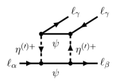
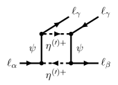
(c) selection of box diagrams

Figure 3: Diagrams contributing to $\ell_{\alpha}\to\ell_{\beta}\bar{\ell}_{\gamma}\ell_{\gamma}$.

This type of process receives in general three independent contributions, shown in Fig. 3, i.e. from $(i)$ $\gamma$-penguin, $(ii)$ $Z$-penguin and $(iii)$ box-type diagrams. We follow the notation of Ref. [21]. The $\gamma$-penguin amplitude for the transition $\ell_{\alpha}(p)\to\ell_{\beta}(k_{1})\,\overline{\ell}_{\gamma}(k_{2})\,\ell_{\gamma}(k_{3})$ is described by

$$\mathcal{A}_{\gamma} = \overline{u}(k_{1})\Big{[}q^{2}\,\gamma^{\rho}\left(A_{1}^{L}\,P_{L}\,+\,A_{1}^{R}\,P_{R}\right)\,+\,m_{\alpha}\,i\,\sigma^{\rho\sigma}\left(A_{2}^{L}\,P_{L}\,+\,A_{2}^{R}\,P_{R}\right)q_{\sigma}\Big{]}u(p)$$ (25)

$$\times\,\frac{e^{2}}{q^{2}}\,\overline{u}(k_{3})\,\gamma_{\rho}\,v(k_{2})\,-\,\left(k_{1}\leftrightarrow k_{3}\right),$$

where $q=p-k_{1}$ and the form factors $A_{1,2}^{L/R}$ are reported in Eq. (19).

The leading order contribution from the $Z$-penguin is proportional to the square of the charged lepton masses and thus negligible compared to the $\gamma$-penguin contribution. There are also box-type diagrams whose contributions are given by

$$\mathcal{A}_{\text{BOX}}\;=\;e^{2}B\,\overline{u}(k_{1})\,\gamma^{\alpha}\,P_{L}\,u(p)\,\overline{u}(k_{3})\,\gamma_{\alpha}\,P_{L}\,v(k_{2})\,,$$ (26)

where for the decay $\ell_{\alpha}^{-}\to\ell_{\beta}^{-}\ell_{\gamma}^{-}\ell_{\gamma}^{+}$ the form factor $B$ reads

$$\begin{split}e^{2}B\;=\;&\frac{1}{16\,\pi^{2}}\Bigg{[}\frac{y_{\Phi}^{\alpha}y_{\Phi}^{\beta*}y_{\Phi}^{\gamma*}y_{\Phi}^{\gamma}}{m_{\eta^{+}}^{2}}\,h_{1}\left(\frac{m_{\psi}^{2}}{m_{\eta^{+}}^{2}}\right)+\frac{y_{\Phi^{\prime}}^{\alpha}y_{\Phi^{\prime}}^{\beta*}y_{\Phi^{\prime}}^{\gamma*}y_{\Phi^{\prime}}^{\gamma}}{m_{\eta^{\prime+}}^{2}}\,h_{1}\left(\frac{m_{\psi}^{2}}{m_{\eta^{\prime+}}^{2}}\right)\Bigg{.}\\ &+\,\Bigg{.}\frac{\left(y_{\Phi}^{\beta*}y_{\Phi^{\prime}}^{\gamma*}+y_{\Phi}^{\gamma*}y_{\Phi^{\prime}}^{\beta*}\right)\left(y_{\Phi^{\prime}}^{\gamma}y_{\Phi}^{\alpha}+y_{\Phi}^{\gamma}y_{\Phi^{\prime}}^{\alpha}\right)}{m_{\psi}^{2}}\,h_{2}\left(\frac{m_{\psi}^{2}}{m_{\eta^{+}}^{2}}\,,\frac{m_{\psi}^{2}}{m_{\eta^{\prime+}}^{2}}\right)\Bigg{]}\,,\end{split}$$ (27)

and for $\ell_{\alpha}^{-}\to\ell_{\gamma}^{-}\ell_{\gamma}^{-}\ell_{\beta}^{+}$ it is given by

$$\begin{split}e^{2}B\;=\;&\frac{1}{16\,\pi^{2}}\Bigg{[}\frac{y_{\Phi}^{\alpha}y_{\Phi}^{\beta}(y_{\Phi}^{\gamma*})^{2}}{m_{\eta^{+}}^{2}}\,h_{1}\left(\frac{m_{\psi}^{2}}{m_{\eta^{+}}^{2}}\right)+\frac{y_{\Phi^{\prime}}^{\alpha}y_{\Phi^{\prime}}^{\beta}(y_{\Phi^{\prime}}^{\gamma*})^{2}}{m_{\eta^{\prime+}}^{2}}\,h_{1}\left(\frac{m_{\psi}^{2}}{m_{\eta^{\prime+}}^{2}}\right)\Bigg{.}\\ &+\,2\Bigg{.}\frac{\left(y_{\Phi}^{\gamma*}y_{\Phi^{\prime}}^{\gamma*}\right)\left(y_{\Phi^{\prime}}^{\beta}y_{\Phi}^{\alpha}+y_{\Phi}^{\beta}y_{\Phi^{\prime}}^{\alpha}\right)}{m_{\psi}^{2}}\,h_{2}\left(\frac{m_{\psi}^{2}}{m_{\eta^{+}}^{2}}\,,\frac{m_{\psi}^{2}}{m_{\eta^{\prime+}}^{2}}\right)\Bigg{]}\,,\end{split}$$ (28)

where all external momenta and masses have been neglected. The loop functions $h_{1}(x)$ and $h_{2}(x,y)$ are given in Eq. (113) in App. D.

One can express the trilepton branching ratios in terms of form factors. Following Ref. [26], the branching ratio of $\ell_{\alpha}\to\ell_{\beta}\,\overline{\ell}_{\beta}\,\ell_{\beta}$ reads

$$\begin{split}\text{BR}(\ell_{\alpha}\to\ell_{\beta}\,\overline{\ell}_{\beta}\,\ell_{\beta})\;=\;&\frac{6\pi^{2}\alpha_{\text{em}}^{2}}{G_{F}^{2}}\Bigg{[}\left|A_{1}^{L}\right|^{2}+\left|A_{2}^{R}\right|^{2}\left(\frac{16}{3}\ln\frac{m_{\alpha}}{m_{\beta}}-\frac{22}{3}\right)\\ &\;+\frac{1}{6}\left|B\right|^{2}-4\,\text{Re}\left(A_{1}^{L*}A_{2}^{R}-\frac{1}{6}\left(A_{1}^{L}-2A_{2}^{R}\right)B^{*}\right)\Bigg{]}\\ &\,\times\text{BR}\left(\ell_{\alpha}\to\ell_{\beta}\,\nu_{\alpha}\,\overline{\nu_{\beta}}\right)\,.\end{split}$$ (29)

For $\ell_{\alpha}^{-}\to\ell_{\beta}^{-}\ell_{\gamma}^{-}\ell_{\gamma}^{+}$, with $\beta\neq\gamma$, the branching ratio is given by

$$\begin{split}\text{BR}(\ell_{\alpha}\to\ell_{\beta}\,\overline{\ell}_{\gamma}\,\ell_{\gamma})\;=\;&\frac{6\pi^{2}\alpha_{\text{em}}^{2}}{G_{F}^{2}}\Bigg{[}\frac{2}{3}\left|A_{1}^{L}\right|^{2}+\left|A_{2}^{R}\right|^{2}\left(\frac{16}{3}\ln\frac{m_{\alpha}}{m_{\gamma}}-8\right)\\ &\;+\frac{1}{12}\left|B\right|^{2}-\frac{8}{3}\,\text{Re}\left(A_{1}^{L}A_{2}^{R*}-\frac{1}{8}\left(A_{1}^{L}-2A_{2}^{R}\right)B^{*}\right)\Bigg{]}\\ &\,\times\text{BR}\left(\ell_{\alpha}\to\ell_{\beta}\,\nu_{\alpha}\,\overline{\nu_{\beta}}\right)\,.\end{split}$$ (30)

For $\ell_{\alpha}^{-}\to\ell_{\beta}^{+}\ell_{\gamma}^{-}\ell_{\gamma}^{-}$, as there are only box-type contributions, we get [26]

$$\begin{split}\text{BR}(\ell_{\alpha}\to\overline{\ell}_{\beta}\,\ell_{\gamma}\,\ell_{\gamma})\;=\;&\frac{\pi^{2}\alpha_{\text{em}}^{2}}{G_{F}^{2}}\left|B\right|^{2}\times\text{BR}\left(\ell_{\alpha}\to\ell_{\beta}\,\nu_{\alpha}\,\overline{\nu_{\beta}}\right)\,.\end{split}$$ (31)

In the dipole dominance approximation, we can express $\mu\to 3e$ in terms of $\mu\to e\gamma$ as

$$\begin{split}\text{BR}(\mu\to 3e)\;\approx\;&\frac{\alpha_{\text{em}}}{8\pi}\,\left(\frac{16}{3}\ln\frac{m_{\mu}}{m_{e}}-\frac{22}{3}\right)\,\times\text{BR}(\mu\to e\,\gamma)\,\\ \;\approx\;&0.006\,\times\text{BR}(\mu\to e\,\gamma)\,.\end{split}$$ (32)

We have checked in the numerical analysis that the above estimate is fulfilled to great precision, confirming that the box-type contributions are not relevant. As the latter involve two extra Yukawa couplings which are smaller than one, the box-type contributions are suppressed with respect to the dipole $A_{2}^{L,R}$ and the monopole $A_{1}^{L,R}$ contributions given in Eq. (19).

The current experimental limit is $\text{BR}(\mu\rightarrow 3e)<1.0\times 10^{-12}$ [27], with an expected future sensitivity of $\sim\mathcal{O}(10^{-16})$ [28]. The other trilepton decays involve $\tau$ leptons, and the upper limits on their branching ratios are $\mathcal{O}(10^{-8})$ [29], with future expected sensitivities of $\sim\mathcal{O}(10^{-9})$ [25].

3.3 $\mu-e$ conversion in nuclei

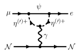
(a) $\gamma$-penguin

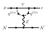
(b) $Z$-penguin

Figure 4: Diagrams contributing to $\mu-e$ conversion in nuclei.

The conversion of a muon to an electron in a nucleus also imposes stringent constraints on the parameter space of the model. This process is dominated by coherent conversions in which initial and final states of the nucleus $\mathcal{N}$ are the same. In this case the matrix elements of the axial-vector $\langle\mathcal{N}|\overline{q}\,\gamma_{\alpha}\,\gamma_{5}\,q|\mathcal{N}\rangle$, pseudoscalar $\langle\mathcal{N}|\overline{q}\,\gamma_{5}\,q|\mathcal{N}\rangle$, and tensor quark currents $\langle\mathcal{N}|\overline{q}\,\sigma_{\alpha\beta}\,q|\mathcal{N}\rangle$ vanish identically [30]. Similar to the leptonic decay of $\tau$ and $\mu$ leptons, the $Z$-penguin contribution to $\mu-e$ conversion in nuclei is proportional to the square of the charged lepton masses and thus negligible compared to the $\gamma$-penguin contribution. See Fig. 4 for the relevant Feynman diagrams. Moreover, the contribution involving the SM Higgs boson is suppressed by the small Yukawa couplings of the first generation of quarks. Thus $\mu-e$ conversion is dominated by photon exchange and the relevant terms in the effective Lagrangian contributing to $\mu-e$ conversion can be parameterised as [30]

$${\cal L}_{\mu-e\,\,\mathrm{conv}} = -\frac{e}{2}\left(m_{\mu}A_{2}^{L}\,\overline{\ell_{e}}\,\sigma^{\mu\nu}P_{L}\,\ell_{\mu}F_{\mu\nu}+m_{\mu}A_{2}^{R}\,\overline{\ell_{e}}\,\sigma^{\mu\nu}P_{R}\,\ell_{\mu}F_{\mu\nu}+{\rm H.c.}\right)$$ (33)

$$-\sum_{q=u,d,s}\left[{\rule[-8.53581pt]{0.0pt}{28.45274pt}\ }\right.\left(g_{LV(q)}^{\gamma}\,\overline{\ell_{e}}\gamma^{\alpha}P_{L}\ell_{\mu}\right)\overline{q}\gamma_{\alpha}q+{\rm H.c.}\left.{\rule[-8.53581pt]{0.0pt}{28.45274pt}\ }\right].\;\;\;\;\;\;\;$$

The long-range interaction mediating the process is given by the electromagnetic dipole transitions, whose form factors $A_{2}^{L/R}$ are introduced in Eq. (19), taking into account the appropriate flavour indices of the Yukawa couplings. The short-range interaction through the $\gamma$-penguin diagrams generate the vector current operator with

$$\begin{split}g_{LV(q)}^{\gamma}\;=\;&e^{2}\,Q_{q}\,A_{1}^{L}\,,\\ \end{split}$$ (34)

where $Q_{q}$ is the electric charge of the quark $q$ in units of $e$ and $A_{1}^{L}$ is the electromagnetic form factor given in Eq. (19) for the flavour indices $\mu$ and $e$. A right-handed leptonic vector current is not induced at one-loop level because all new particles exclusively couple to the left-handed lepton doublets $L_{\alpha}$. Accordingly, the $\mu-e$ conversion rate is given in terms of the overlap integrals $D$ and $V^{(p,n)}$ as

$$\omega_{\rm conv}\;=\; 4\,\left|\frac{e}{8}A_{2}^{R}D+\tilde{g}_{LV}^{(p)}V^{(p)}+\tilde{g}_{LV}^{(n)}V^{(n)}\right|^{2}\ ,$$ (35)

where the effective vector couplings $\tilde{g}_{LV}^{(p,n)}$ for the proton and the neutron are

$$\tilde{g}_{LV}^{(p)} \approx 2\,g_{LV(u)}^{\gamma}+g_{LV(d)}^{\gamma}=e^{2}A_{1}^{L}\ , \tilde{g}_{LV}^{(n)} \approx g_{LV(u)}^{\gamma}+2\,g_{LV(d)}^{\gamma}=0\,.$$ (36)

Notice that the neutron contribution is in our case approximately zero, as we neglected the $Z$-penguin contribution.

We can express $\omega_{\rm conv}$ in terms of $\text{BR}(\mu\to e\,\gamma)$ using that

$$A_{1}^{L}\approx\frac{2}{3}\,r_{g/f}\,A_{2}^{R}\,,$$ (37)

where $r_{g/f}$ parametrises the difference due to the different loop functions with $1\lesssim r_{g/f}\lesssim 1.5$ for $x\lesssim 1$ ($m_{\psi}$ is always smaller than $m_{\eta^{(\prime)+}}$, since $\psi$ is the DM candidate), see Eqs. (19) and (112). In this case we can derive the allowed ranges for

$$\text{CR}_{\rm conv} \equiv \frac{\omega_{\rm conv}}{\omega_{\rm capt}}$$ (38)

$$\approx \;\frac{G_{F}^{2}}{192\,\pi^{2}\,\omega_{\rm capt}}\,\left|D+\frac{16}{3}\,r_{g/f}\,e\,V^{(p)}\right|^{2}\,\times\text{BR}(\mu\to e\,\gamma)$$

$$\approx \;[0.0077,0.011]\,([0.010,0.015])\,\{[0.013,0.019]\}\,\times\text{BR}(\mu\to e\,\gamma)\,,$$

for   Al  (Au) {Ti}. Here we used the numerical values of the overlap integrals $D$ and $V^{(p,n)}$ and the total capture rate $\omega_{\rm capt}$ reported in Tab. 5 in App. D. We have checked that the numerical results for the $\mu-e$ conversion ratio (CR) are in very good agreement with the estimates in Eq. (38), see Figs. 10 and 12.

The currently best experimental limits are set by the SINDRUM II experiment [31]: $\mathrm{CR}_{\rm conv}(\rm Au)<7\cdot 10^{-13}$ and $\mathrm{CR}_{\rm conv}(\rm Ti)<4.3\cdot 10^{-12}$ at 90 % CL. Future experiments are expected to improve the sensitivity by several orders of magnitude: the COMET experiment at J-PARC [32, 33] may improve down to $\mathcal{O}(10^{-17})$, Mu2e experiment at Fermilab using Al [34, 35, 36] $6\cdot 10^{-17}$ and at Project X (Al or Ti) $\mathcal{O}(10^{-19})$, and PRISM/PRIME [37, 38] may reach $\mathcal{O}(10^{-18})$.

3.4 Lepton dipole moments

Contributions to the electric dipole moments of charged leptons arise in the model only at the two-loop level. However, non-zero contributions to leptonic magnetic dipole moments are generated, similarly to contributions to radiative CLFV decays, at one-loop level. The relevant Feynman diagram is shown in Fig. 2 for $\alpha=\beta$. They receive two independent contributions from the charged scalars $\eta^{\pm}$ and $\eta^{\prime\pm}$ running in the loop. They are given by (see also Refs. [40, 41])

$$\Delta a_{\ell}\equiv\frac{g_{\ell}-2}{2}\;=\;2\,m^{2}_{\ell}\,{\rm Re}[A_{2}^{R}]_{\ell}\,,$$ (39)

where $[A_{2}^{R}]_{\ell}$ is the diagonal part ($\alpha=\beta\equiv\ell$) of the coefficient $A_{2}^{R}$ given in Eq. (19).

In the case of the anomalous muon magnetic dipole moment $\Delta a_{\mu}$, the discrepancy between the measured value and the one predicted within the SM is larger than zero (see Ref. [42] for a recent review), and therefore the model cannot explain it, as it gives a negative contribution, see Eq. (19) together with the loop function $f(x)>0$. In any case, the predictions for $|\Delta a_{\mu}|$ are always small, $|\Delta a_{\mu}|\lesssim 10^{-12}$, as long as limits imposed by the non-observation of CLFV decays are fulfilled. The magnetic dipole moments of the electron and the $\tau$ lepton are subject to very weak limits.

3.5 Dark matter relic abundance

We study the case where the DM candidate is the Dirac fermion $\psi$. There are several possible production channels in the early Universe. In particular the value of the Yukawa couplings of the fermionic singlet control the different regimes, see also Ref. [43]: (i) If the Yukawa couplings are very small ($\ll 1$), direct annihilations of the scalars dominate the relic abundance. (ii) For intermediate values, fermion–scalar coannihilations dominate and set the relic abundance. (iii) For larger values, annihilations of the fermion would in principle dominate.

In the next subsection we argue that DM annihilations to SM leptons $\psi\bar{\psi}\to\ell\bar{\ell},\nu\bar{\nu}$ (regime 3) are too small due to constraints from CLFV processes. We show in Fig. 5(a) the $t$-channel annihilations mediated by $\eta^{\pm},\,\eta_{0}^{\prime}$. The correct relic abundance is set by coannihilations (regimes 1 and 2), see the diagrams in Figs. 5(b) and 5(c). The latter are possible if the relative mass splitting between the fermion and the scalars is smaller or equal than $5\%$.

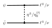
(a) Annihilations of dark matter into leptons.

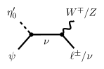
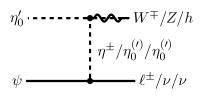
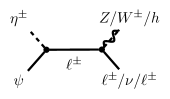
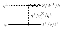
(b) Coannihilations of dark matter with a new scalar.

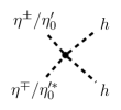
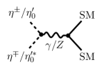
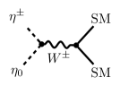
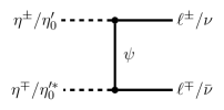
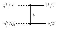
(c) Annihilations of the scalar coannihilation partners.

Figure 5: Illustration of the relevant annihilation (top panel) and coannihilation (middle panel) channels of the dark matter $\psi$ involving the scalars $\eta^{\pm},\,\eta_{0}^{\prime}$. We also show diagrams of the annihilation channels of the coannihilating partners $\eta^{\pm},\,\eta_{0}^{\prime}$ (bottom panel). More diagrams exist involving the other new scalars.

3.5.1 Dark matter annihilations

The dominant DM annihilation channels are into a pair of charged leptons or a pair of neutrinos, shown in Fig. 5(a). In the non-relativistic limit the $s$-wave annihilation cross sections to neutrinos and charged leptons are given by

$$\left\langle v\sigma(\psi\bar{\psi}\to\ell_{\alpha}^{-}\ell_{\beta}^{+})\right\rangle \simeq\frac{1}{32\pi m_{\psi}^{2}}\left|y_{\Phi}^{\alpha}y_{\Phi}^{\beta*}\frac{m_{\psi}^{2}}{m_{\eta^{+}}^{2}+m_{\psi}^{2}}-y_{\Phi^{\prime}}^{\alpha}y_{\Phi^{\prime}}^{\beta*}\frac{m_{\psi}^{2}}{m_{\eta^{\prime+}}^{2}+m_{\psi}^{2}}\right|^{2}\,,$$ (40)

$$\left\langle v\sigma(\psi\bar{\psi}\to\nu_{\alpha}\nu_{\beta})\right\rangle \simeq\frac{1}{64\pi m_{\psi}^{2}(1+\delta_{\alpha\beta})}\left|y_{\Phi}^{\alpha}y_{\Phi}^{\beta*}\left(\frac{m_{\psi}^{2}s_{\theta}^{2}}{m_{\eta_{0}}^{2}+m_{\psi}^{2}}+\frac{m_{\psi}^{2}c_{\theta}^{2}}{m_{\eta_{0}^{\prime}}^{2}+m_{\psi}^{2}}\right)\right.$$ (41)

$$\hskip 85.35826pt\left.-y_{\Phi^{\prime}}^{\alpha}y_{\Phi^{\prime}}^{\beta*}\left(\frac{m_{\psi}^{2}c_{\theta}^{2}}{m_{\eta_{0}}^{2}+m_{\psi}^{2}}+\frac{m_{\psi}^{2}s_{\theta}^{2}}{m_{\eta_{0}^{\prime}}^{2}+m_{\psi}^{2}}\right)\right|^{2}\,.$$

The minus sign between the different contributions originates from the presence of $t$- and $u$-channel diagrams mediated by $\eta$ and $\eta^{\prime}$, respectively. As neutrinos are Majorana particles, the corresponding cross section is smaller by a factor of two. For identical neutrinos in the final state $\delta_{\alpha\beta}=1$ which leads to another factor of $1/2$.

Next we conservatively estimate these cross sections in the limit of large and small $|\zeta|$ using the obtained limits on $|\zeta|$ in Eq. (24). In the limit of equal masses, denoted by $m$, the cross sections only depend on whether primed or unprimed Yukawa couplings are present. Larger scalar masses only further suppress the annihilation cross section. Thus we obtain the following conservative limit

$$\sum_{\alpha,\beta}\left\langle v\sigma(\psi\bar{\psi}\to\ell_{\alpha}^{-}\ell_{\beta}^{+},\nu_{\alpha}\nu_{\beta})\right\rangle \lesssim\sum_{\alpha,\beta}\frac{\left|y_{\Phi^{(\prime)}}^{\alpha}y_{\Phi^{(\prime)}}^{\beta*}\right|^{2}}{256\pi\,m^{2}}\frac{3+2\delta_{\alpha\beta}}{1+\delta_{\alpha\beta}}\,.$$ (42)

This allows us to use the limit on $|\zeta|$ from Eq. (24). A comparison to the typical freeze-out annihilation cross section, $\left\langle v\sigma\right\rangle_{\rm th}\simeq 2.2\times 10^{-26}\,{\rm cm^{3}/s}$, yields that the DM annihilation cross section is always too small in order for the Dirac fermion $\psi$ to account for the observed relic density. Using the experimental upper limit on the branching ratio for $\mu\to e\gamma$ on the parameter $|\zeta|$ in Eq. (24), we obtain

$$\sum_{\alpha,\beta}\left\langle v\sigma(\psi\bar{\psi}\to\ell_{\alpha}^{-}\ell_{\beta}^{+},\nu_{\alpha}\nu_{\beta})\right\rangle \lesssim 2\times 10^{-4}\left(\frac{\left\langle v\sigma\right\rangle_{\rm th}}{2.2\times 10^{-26}\,\mathrm{cm}^{3}\,\mathrm{s}^{-1}}\right)\left(\frac{m}{100\,\mathrm{GeV}}\right)^{4}$$ (43)

for any neutrino mass ordering, which is valid unless cancellations occur.

An interesting way to break the correlation of ${\rm BR}(\ell_{\alpha}\to\ell_{\beta}\,\gamma)$ and DM annihilation cross section is to have the DM relic abundance set by $\left\langle v\sigma(\psi\bar{\psi}\to\nu\bar{\nu})\right\rangle$. This can be achieved if the charged scalars $\eta^{\pm}$ and $\eta^{\prime\pm}$ are much heavier than at least one neutral scalar ($\eta^{\prime}_{0}$ in this model), leading therefore to suppressed contributions to all radiative CLFV processes, and also to $\left\langle v\sigma(\psi\bar{\psi}\to\ell^{-}\ell^{+})\right\rangle$. In this scenario the mass of the Dirac fermion DM $\psi$ is typically in the MeV range to obtain the correct DM relic density, with slightly heavier neutral scalar $\eta_{0}^{\prime}$. However, gauge invariance relates the interactions of neutrinos and charged leptons, and therefore this scenario requires some tuning of the parameters in order to circumvent experimental constraints from $Z$-boson decays, the $T$ parameter and CLFV processes. We thus do not consider it any further. Examples of similar scenarios have been studied in Refs. [44, 45, 46, 47].

3.5.2 Dark matter coannihilations

As DM annihilation into charged leptons and neutrinos is strongly constrained by experimental limits on CLFV observables, coannihilation processes may become important. The explanation of the correct DM relic abundance requires a small mass splitting between the DM candidate $\psi$ and the scalars $\eta_{0}^{\prime}$ and $\eta^{(\prime)+}$. While this is perfectly plausible in the model, in which the particles naturally are at the TeV scale, in its current version there is no symmetry or dynamic reason to generate similar scalar and fermion masses. Another option is a variant of the model with an fermionic electroweak triplet instead of a singlet, discussed in Sec. 5.3. This allows to have the relic abundance set by annihilations, without the need of coannihilations. The relative contribution of $(i)$ annihilations of the DM particle with the coannihilation partner into a lepton and a gauge boson or Higgs boson (see Fig. 5(b)), and $(ii)$ annihilations of the coannihilation partner(s) via gauge interactions ($\gamma/Z/W$) into SM particles, direct annihilations to Higgs bosons or DM-mediated $t$-channel annihilations into leptons (shown in Fig. 5(c)), depends on the size of the Yukawa couplings and the mass splitting. The coannihilation channels dominate the abundance, because the corresponding cross sections only depend on the square of one of the Yukawa couplings $y_{\Phi}^{\alpha},\,y_{\Phi^{\prime}}^{\alpha}$ compared to the annihilation cross section, see Eq. (40) and (41), which involves four Yukawa couplings. In our numerical scan we use micrOMEGAs 4.3.5 [48] to calculate the DM relic abundance and thus take all relevant (co)annihilation channels into account. See the seminal work [49] by K. Griest and D. Seckel for an analytic discussion of coannihilation.

3.6 Dark matter direct detection

One of the interesting features of the GScM is that the fermionic DM candidate $\psi$ is a Dirac fermion rather than a Majorana fermion as in the original ScM. A direct detection (DD) signal can not be generated at tree level, but there are sizeable long-range contributions at the one-loop level via photon exchange. It can be parameterised by the magnetic (and electric) dipole interactions, namely

$$\mathcal{L}_{\mathrm{DD}} =\mu_{\psi}\frac{e}{8\pi^{2}}\bar{\psi}\sigma_{\mu\nu}\psi F^{\mu\nu}+d_{\psi}\frac{e}{8\pi^{2}}\bar{\psi}\sigma_{\mu\nu}i\gamma_{5}\psi F^{\mu\nu}\,.$$ (44)

In this model the electric dipole moment $d_{\psi}$ vanishes at one-loop level, because $\psi$ only couples to left-handed lepton doublets and not to right-handed charged leptons simultaneously [50]. The magnetic dipole moment $\mu_{\psi}$ is given by

$$\mu_{\psi} =\frac{-1}{4m_{\psi}}\sum_{\alpha}\Big{(}\left|y_{\Phi}^{\alpha}\right|^{2}f_{\rm DD}(m_{\psi},m_{\eta^{+}},m_{\ell_{\alpha}})-\left|y_{\Phi^{\prime}}^{\alpha}\right|^{2}f_{\rm DD}(m_{\psi},m_{\eta^{\prime+}},m_{\ell_{\alpha}})\Big{)}\;.$$ (45)

The loop function $f_{\mathrm{DD}}(x,y,z)$ is defined in Eq. (114) in App. D. We checked our result against the well-known expressions for the magnetic dipole moment for a Yukawa interaction found in Ref. [51]. Similar results are given in Refs. [52, 53, 54, 9, 55, 56, 50]. In Fig. 12 in Sec. 4 we show how results from the latest Xenon experiments XENON1T [57], PandaX-II [58], and LUX [59] constrain the parameter space of the model using LikeDM [60].

3.7 Electroweak precision tests

The dominant contribution from new physics to electroweak radiative processes is generally expected to affect the gauge boson self-energies which are parameterised by the oblique parameters $S$, $T$, and $U$ [61, 62]. The limits on the oblique parameters are obtained from a global fit to electroweak precision data. The Gfitter collaboration finds the values: $S=0.05\pm 0.11$, $T=0.09\pm 0.13$ and $U=0.01\pm 0.11$, with correlation coefficients $\rho_{\rm ST}=0.90$, $\rho_{\rm SU}=-0.59$ and $\rho_{\rm TU}=-0.83$ [63]. The strongest constraints on the parameter space of the model are set by the $T$ parameter, which is sensitive to the mass splitting between the neutral and charged scalar components of the two inert doublets $\Phi$ and $\Phi^{\prime}$. We use the expressions for the oblique parameters found in Refs. [64, 65, 66]. Details are reported in App. E.

3.8 Production and decay of the new scalars at colliders

Searches for neutral and charged scalars at colliders set constraints on the scalar mass spectrum of the model. In fact, from the precise measurement of the $W$ and $Z$ boson decay widths at LEP-II, the following kinematical bounds can be derived: $m_{\eta_{0}^{(\prime)}}+m_{\eta^{(\prime)+}}>m_{W}$ and $2m_{\eta^{(\prime)+}},2m_{\eta_{0}^{(\prime)}},m_{\eta_{0}}+m_{\eta_{0}^{\prime}}>m_{Z}$ for $m_{W(Z)}$ being the $W$ ($Z$) boson mass.

At the LHC the production of these states proceeds mainly via neutral and charged current Drell-Yan processes. Other production channels are via an off-shell $Z/W$ boson. A sub-leading contribution is given by Higgs mediated gluon fusion, provided the relevant couplings in the scalar potential in Eq. (3) are sizeable [67, 4].

In the case one of the charged scalars is the next-to-lightest particle in the dark sector, the expected signature at the LHC consists in the pair production of $\eta^{(\prime)\pm}$ followed by the prompt decay $\eta^{(\prime)\pm}\to\psi\ell_{\alpha}^{\pm}$ ($\alpha=e,\mu,\tau$). The DM particle $\psi$ escapes the detector and is revealed as missing transverse energy. The decay branching ratios of $\eta^{(\prime)\pm}$ into the different leptons only depend on the neutrino Yukawa couplings, namely

$$\text{BR}(\eta^{(\prime)\pm}\to\psi\,\ell_{\alpha}^{\pm})\;=\;\frac{\Gamma(\eta^{(\prime)\pm}\rightarrow\psi\ell_{\alpha}^{\pm})}{\sum_{\beta}\Gamma(\eta^{(\prime)\pm}\rightarrow\psi\,\ell_{\beta}^{\pm})}=\frac{|y_{\Phi^{(\prime)}}^{\alpha}|^{2}}{\sum_{\beta}|y_{\Phi^{(\prime)}}^{\beta}|^{2}}\,.$$ (46)

Using the estimates for $y^{\alpha}_{\Phi}$ and $y^{\alpha}_{\Phi^{\prime}}$ reported in Sec. 2.2 we expect for neutrino masses with NO that both charged scalars $\eta^{\pm}$ and $\eta^{\prime\pm}$ have very similar branching ratios with the one to $e^{\pm}$ being suppressed by two powers of the reactor mixing angle $\theta_{13}$ with respect to those to $\mu^{\pm}$ and $\tau^{\pm}$. Since $\theta_{23}\approx\pi/4$, the branching ratios to the two flavours $\mu^{\pm}$ and $\tau^{\pm}$ are expected to be very similar for both NO and IO, see Eqs. (15) and (17), respectively. Moreover, for neutrino masses with IO the branching ratios of both charged scalars $\eta^{\pm}$ and $\eta^{\prime\pm}$ to $\mu^{\pm}$ and $\tau^{\pm}$ are expected to be very similar, whereas the ones to $e^{\pm}$ are expected to be different, but of similar size. In particular, we note that for IO ${\rm BR}(\eta^{\pm}\to\psi\,e^{\pm})\approx 2\,{\rm BR}(\eta^{\prime\pm}\to\psi\,\mu^{\pm}(\tau^{\pm}))$ and ${\rm BR}(\eta^{\prime\pm}\to\psi\,e^{\pm})\approx 2\,{\rm BR}(\eta^{\pm}\to\psi\,\mu^{\pm}(\tau^{\pm}))$. A measurement of at least one of the branching ratios may allow to extract information on the neutrino mass ordering and the Majorana phase $\gamma$, while there is only a weak dependence on the Dirac phase $\delta$.

In the coannihilation region corresponding to $m_{\eta_{0}^{(\prime)}}>m_{\eta^{(\prime)+}}\gtrsim m_{\psi}$, the decay width of the charged scalar is kinematically suppressed. As we discuss in the numerical analysis in Sec. 4, in this case the lightest charged scalar may be long-lived, leaving ionising tracks in the detector [43, 4].

3.9 Decays of the Higgs and $Z$ bosons

If the scalars are sufficiently light, the Higgs and $Z$ bosons can decay into them at tree level which is strongly experimentally constrained. In specific cases some of the limits on the neutral scalar masses from $Z$ decays can be evaded by tuning the mixing angle $\theta$, see Eq. (7). For instance, the $Z$-boson decay rate into the lightest neutral scalar, $\Gamma(Z\to\eta_{0}^{\prime}\eta^{\prime*}_{0})$, is proportional to $\cos^{2}(2\theta)$ and therefore vanishes in the case of maximal mixing, $\theta=\pi/4$. In this case the mass of the lightest neutral scalar, $m_{\eta_{0}^{\prime}}$, can be smaller than $m_{Z}/2$. For the Higgs boson the decay to the lightest neutral scalar can be suppressed for sufficiently small quartic couplings and/or a suitable choice of the mixing angle $\theta$.

There can also be Higgs and $Z$-boson decays at one-loop level. The charged scalars couple to the Higgs boson and thus modify the decay of the Higgs boson to two photons. The relative change of the Higgs partial decay width to two photons compared to the SM prediction can be parameterised as [70, 71, 72]

$$R_{\gamma\gamma}=\frac{{\rm BR}(h\rightarrow\gamma\gamma)_{\rm GScM}}{{\rm BR}(h\rightarrow\gamma\gamma)_{\rm SM}}\simeq\left|1+\frac{\frac{\lambda_{H\Phi}\,v_{H}^{2}}{2\,m_{\eta^{+}}^{2}}\,A_{0}\left(\frac{4m_{\eta^{+}}^{2}}{m_{h}^{2}}\right)+\frac{\lambda_{H\Phi^{\prime}}v_{H}^{2}}{2\,m^{2}_{\eta^{\prime+}}}\,A_{0}\left(\frac{4m_{\eta^{\prime+}}}{m_{h}^{2}}\right)}{A_{1}\left(\frac{4m_{W}^{2}}{m_{h}^{2}}\right)+\frac{4}{3}A_{1/2}\left(\frac{4m_{t}^{2}}{m_{h}^{2}}\right)}\right|^{2}\,,$$ (47)

where $\lambda_{H\Phi},\lambda_{H\Phi^{\prime}}$ are the couplings of the charged scalars $\eta^{+},\,\eta^{\prime+}$ to the Higgs boson, see Eq. (3). $A_{i}(x)$ are loop functions for scalars, fermions and gauge bosons with $(i=0,1/2,1)$ respectively, given in Eq. (115) in App. D. $m_{t}$ is the top quark mass. The ATLAS and CMS experiments have measured the partial width of $h\rightarrow\gamma\gamma$ and reported it in terms of the signal strength $\mu_{\gamma\gamma}\equiv R_{\gamma\gamma}\sigma(pp\to h)/\sigma(pp\to h)_{\rm SM}$. As the new particles are not coloured and thus the Higgs production cross section is unchanged the signal strength is simply given by $\mu_{\gamma\gamma}=R_{\gamma\gamma}$ in this model. ATLAS observes $\mu_{\gamma\gamma}=1.14^{+0.27}_{-0.25}$ [73], and CMS $\mu_{\gamma\gamma}=1.11^{+0.25}_{-0.23}$ [74] which can be interpreted as a constraint on the charged scalars. The combined measurement is $\mu_{\gamma\gamma}=1.14^{+0.19}_{-0.18}$ [75]. If the charged scalar masses are light enough, deviations in the $h\rightarrow\gamma\gamma$ channel are generically expected, but their size crucially depends on parameters in the scalar potential, see Eq. (3) As observed in the numerical scan, this constraint can be fulfilled in the GScM.

In principle, there can be new invisible decay channels of the Higgs and $Z$ bosons to the DM particle $\psi$ as well as of the Higgs to neutrinos. Generically, the new scalars are constrained to be heavier than $\sim 100$ GeV due to a combination of collider searches, the limits from the invisible decay width of the $Z$ boson, and EWPT. Consequently, also the DM particle $\psi$ cannot be light in the case of coannihilations, see Sec. 3.5, and thus the Higgs and the $Z$ bosons cannot decay into $\psi$, which would otherwise occur at one-loop level, see Ref. [50].

Other possible processes are CLFV (and lepton flavour universality violating) Higgs and $Z$-boson decays, like $h\rightarrow\tau\mu$ and $Z\rightarrow\tau\mu$. These, however, are very suppressed by a loop factor and due to experimental constraints arising from other CLFV processes (like $\tau\rightarrow\mu\gamma$). They are therefore well beyond the expected sensitivity of future experiments [76].

4 Numerical analysis

The Yukawa couplings of the model are determined by neutrino oscillation data, the Majorana phase $\gamma$ and the parameter $\zeta$ (which can be taken positive without loss of generality), as explained in App. C. We scan over the 3$\sigma$ range of the neutrino oscillation parameters using the results from NuFIT 3.1 (November 2017) [77, 78], reproduced for convenience in Tab. 2, as well as over the rest of the parameters of the model and $\zeta$ as outlined in Tab. 3. The points indicate the currently allowed parameter space. The varying density of points is mostly due to the efficiency of the scan and does not have a meaningful statistical interpretation.

Observable	NO	IO
$\sin^{2}\theta_{12}$	$[0.272,0.347]$	$[0.272,0.347]$
$\sin^{2}\theta_{23}$	$[0.401,0.628]$	$[0.419,0.628]$
$\sin^{2}\theta_{13}$	$[0.01971,0.02434]$	$[0.01990,0.02437]$
$\Delta m^{2}_{21}/10^{-5}\,[{\rm eV}^{2}]$	$[6.80,8.02]$	$[6.80,8.02]$
$\Delta m^{2}_{3\ell}/10^{-3}\,[{\rm eV}^{2}]$	$[2.408,2.621]$	$[-2.589,-2.379]$
$\delta$ $[{}^{\circ}]$	$[0,30]\cup[128,360]$	$[0,7]\cup[182,360]$
$\gamma$ $[{}^{\circ}]$	$[0,180]$	$[0,180]$

Table 2: The $3\sigma$ ranges for the lepton mixing parameters and mass-squared differences from NuFIT 3.1 (November 2017) [77, 78]. Here $\Delta m^{2}_{3\ell}=\Delta m^{2}_{31}>0$ for normal ordering (NO) and $\Delta m^{2}_{3\ell}=\Delta m^{2}_{32}<0$ for inverted ordering (IO). We scan over these using flat priors.

Parameter	Range
$\lambda_{i}$	$\pm$$[10^{-3},4\pi]$
$\lambda_{H\Phi\Phi^{\prime}}$	$[10^{-8},4\pi]$
$m_{\Phi^{(\prime)}}$ [GeV]	$[100,10^{5}]$
$m_{\psi}$ [GeV]	$[10,10^{5}]$
$\zeta$	$[10^{-3},10^{3}]$

Table 3: Priors on the 12 free real parameters used in the scan. $\lambda_{i}$ includes the following 8 quartic couplings of the potential: $\lambda_{\Phi^{(\prime)}},\,\lambda_{H\Phi^{(\prime)}},\,\lambda_{H\Phi^{(\prime)},2},\,\lambda_{\Phi\Phi^{\prime}},\,\lambda_{\Phi\Phi^{\prime},2}$. The parameter $\zeta$ is defined in App. C. We scan over these parameters using logarithmic priors.

We impose several constraints directly in the scan: $(i)$ Direct searches for singly-charged scalars from LEP II imply $m_{\eta^{({\prime})+}}\gtrsim 100$ GeV, with some dependence on the search channel; $(ii)$ constraints from the Higgs or $Z$-boson decay widths and $(iii)$ $3\sigma$ constraints from EWPT, see Sec.  3.7. These constraints restrict the mass splittings of the scalars, specially the one from the $T$ parameter; thus we also impose a lower bound of 100 GeV for all the new scalars; $(iv)$ we apply the stability conditions on the scalar potential given in App. A; $(v)$ we use the experimental limits on the branching ratios from radiative $\ell_{\alpha}\rightarrow\ell_{\beta}\gamma$; $(vi)$ we assume that the Dirac fermion $\psi$ constitutes all of the DM in the Universe and thus require its relic abundance to lie within the $3\sigma$ range of the latest results from Planck [79], $\Omega_{\rm DM}h^{2}=0.1198\pm 0.0026$. All the observables for which we impose constraints in the numerical scan are provided in Tab. 4.

Observable	Upper bound	Observable	Measurement
$\mathrm{Br}(\mu^{+}\to e^{+}\gamma)$	$2.55\cdot 10^{-13}$ [23]	$S$	$0.05\pm 0.11$ [63]
$\mathrm{Br}(\tau^{-}\to\mu^{-}\gamma)$	$4.4\cdot 10^{-8}$ [22]	$T$	$0.09\pm 0.13$ [63]
$\mathrm{Br}(\tau^{-}\to e^{-}\gamma)$	$3.3\cdot 10^{-8}$ [22]	$U$	$0.01\pm 0.11$ [63]
$\sum m_{i}$ $[\mathrm{eV}]$	$0.23$ [79]	$\Omega_{\rm DM}\,h^{2}$	$0.1198\pm 0.0026$ [79]

Table 4: The current experimental upper bounds (two left columns) at 90% CL and the measurements with their errors (two right columns) used in the parameter scan. They are required to lie within the $3\sigma$ range for the measurements. The correlation coefficients for the oblique parameters are $\rho_{ST}=0.90$, $\rho_{SU}=-0.59$ and $\rho_{TU}=-0.83$. [63]

In the following subsections we show the results of a numerical scan with about $10^{4}$ random points, using the input parameters in Tabs. 2 and 3. Most of the results are shown for NO. Those for IO, unless explicitly shown, are basically identical.

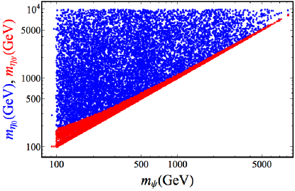
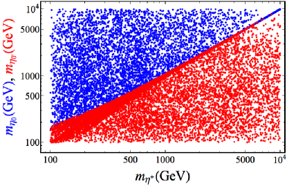
Figure 6: The lighter and heavier neutral scalar masses, $m_{\eta^{\prime}_{0}}$ and $m_{\eta_{0}}$, in red and blue, respectively, versus the dark matter mass $m_{\psi}$ in the left panel, and versus the charged scalar mass $m_{\eta^{+}}$ in the right panel.

4.1 Masses and lifetimes of the new scalars

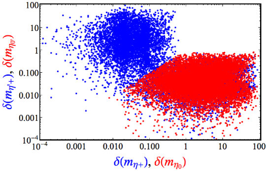
Figure 7: Normalised mass splitting $\delta(m_{x})=(m_{x}-m_{\psi})/m_{\psi}$ of the charged scalar $\eta^{\prime+}$ versus $\eta^{+}$, in blue, and of the neutral scalar $\eta_{0}^{\prime}$ versus $\eta_{0}$, in red. Notice that the red region of points is superimposed over part of the blue one.

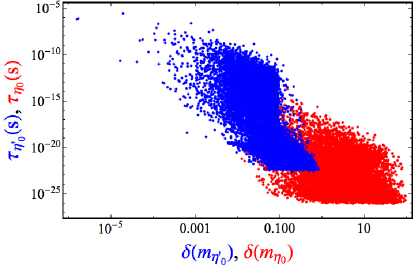
Figure 8: Left panel: Lifetime of the neutral scalars $\eta_{0}^{\prime}$ (blue) and $\eta_{0}$ (red) versus the normalised mass splitting $\delta(m_{x})=(m_{x}-m_{\psi})/m_{\psi}$. Right panel: Lifetime of the charged scalar $\eta^{+}$ versus $\delta(m_{\eta^{+}})$ for different ranges of $\lambda_{H\Phi\Phi^{\prime}}$. We indicate with a horizontal dotted black line the minimum lifetime needed for the charged scalar to be long-lived at collider scales. A similar plot is obtained for the charged scalar $\eta^{\prime+}$.

Figure 9: Left panel: $|\mathbf{y_{\Phi^{\prime}}}|$ versus $|\mathbf{y_{\Phi}}|$ for different ranges of $\lambda_{H\Phi\Phi^{\prime}}$. Right panel: $|\mathbf{y_{\Phi}}||\mathbf{y_{\Phi^{\prime}}}|$ versus the mass splitting of the new neutral scalars $m_{\eta_{0}}-m_{\eta^{\prime}_{0}}$ for different ranges of $|\sin 2\theta|$.

We show in Fig. 6 (left panel) the lightest and the heaviest neutral scalar masses, $m_{\eta^{\prime}_{0}}$ and $m_{\eta_{0}}$, versus the DM mass $m_{\psi}$, in red and blue, respectively. The lightest neutral scalar mass is close to the DM mass. This is driven by the fact that coannihilations need to be efficient enough in order to obtain the correct relic abundance. In Fig. 6 (right panel), we show the neutral scalar masses versus the charged scalar mass $m_{\eta^{+}}$. We observe that $\eta_{0}$ is always the heaviest state. Roughly in 50% (30%) of the points the mass of the lightest neutral (one of the charged) scalar(s) is very degenerate with the mass of the DM particle (with a normalised mass splitting smaller than $5\%$) and contributes to coannihilations. In addition, there are significant regions of the parameter space of the model (18% of the points) where both masses of lightest neutral and one of the charged scalars ($\eta^{\pm}$ or $\eta^{\prime\pm}$) are nearly degenerate with the DM mass. Only in around $1\%$ of the points the masses of the three new scalars $\eta^{\prime}_{0},\,\eta^{\pm},\,\eta^{\prime\pm}$ are very degenerate with the DM mass. There is no difference between the cases with neutrinos with NO and IO.

In Fig. 7 we show the normalised mass splitting $\delta(m_{x})=(m_{x}-m_{\psi})/m_{\psi}$ of the charged scalars, $\eta^{\prime+}$ versus $\eta^{+}$, in blue, and of the neutral scalars, $\eta_{0}^{\prime}$ versus $\eta_{0}$, in red. Notice that the red region of points is superimposed over part of the blue one. The normalised mass splitting $\delta(m_{x})=(m_{x}-m_{\psi})/m_{\psi}$ needs to be below $\sim 50\%$, and typically $\sim 5\%$, for at least one of the scalars $\eta_{0}^{\prime}$, $\eta^{\pm}$ and/or $\eta^{\prime\pm}$ in order for coannihilations to be efficient. It is typically much larger for the heaviest neutral scalar $\eta_{0}$, as can be seen in Fig. 7.

In Fig. 8 (left panel) we plot the lifetime of the neutral scalars, $\eta_{0}^{\prime}$ (blue) and $\eta_{0}$ (red), versus the normalised mass splitting $\delta(m_{x})=(m_{x}-m_{\psi})/m_{\psi}$. One can observe how the lifetime of $\eta_{0}^{\prime}$ can be much larger than that of $\eta_{0}$. Indeed, when the splitting $\delta(m_{\eta^{\prime}_{0}})$ with the DM mass is small, the only decays of $\eta_{0}^{\prime}$ are into charged leptons, and even those can be impossible for very small mass splittings and/or suppressed for small Yukawa couplings. In Fig. 8 (right panel) we plot the lifetime of the charged scalar $\eta^{+}$ versus $\delta(m_{\eta^{+}})$, for different ranges of $\lambda_{H\Phi\Phi^{\prime}}$: $10^{-8}\lesssim\lambda_{H\Phi\Phi^{\prime}}\lesssim 0.01$ in red, $0.01\lesssim\lambda_{H\Phi\Phi^{\prime}}\lesssim 0.5$ in blue, and $0.5\lesssim\lambda_{H\Phi\Phi^{\prime}}\lesssim 4\pi$ in green. The plot for the charged scalar $\eta^{\prime+}$ is analogous to that of $\eta^{+}$. We observe two effects: firstly, for large mass splittings, $\delta(m_{\eta^{+}})\gtrsim 0.1$ which corresponds to $m_{\eta^{+}}-m_{\psi}\gtrsim 80$ GeV, the main decay channel is $\eta^{+}\rightarrow W^{+}\eta_{0}^{\prime}$, and the larger the quartic coupling $\lambda_{H\Phi\Phi^{\prime}}$, the larger the neutral scalars mixing $\cos\theta$, see Eq. (7), and the larger this decay; secondly, the larger the normalised mass splitting with the DM mass, the smaller the lifetime. Indeed, the charged scalar can be long-lived at collider scales, meaning $\tau_{\eta^{+}}\gtrsim 10^{-8}$ s, as shown with a horizontal dotted black line for mass splittings $m_{\eta^{+}}-m_{\eta^{\prime}_{0}}$ smaller than $\sim 80$ GeV, when the decay channel $\eta^{+}\rightarrow W^{+}\eta_{0}^{\prime}$ is closed. In that region, the decays $\eta^{+}\rightarrow\ell_{\alpha}^{+}\psi$, that are mediated by the Yukawa couplings $y^{\alpha}_{\Phi}$, dominate. Therefore, the larger the quartic coupling $\lambda_{H\Phi\Phi^{\prime}}$, the smaller the Yukawa couplings, and the larger the lifetime, see blue and green points in Fig. 8 (right panel).

4.2 Neutrino Yukawa couplings

In the left panel of Fig. 9 we show $|\mathbf{y_{\Phi^{\prime}}}|$ versus $|\mathbf{y_{\Phi}}|$ for fixed intervals of $\lambda_{H\Phi\Phi^{\prime}}$: $10^{-8}\lesssim\lambda_{H\Phi\Phi^{\prime}}\lesssim 0.01$ in red, $0.01\lesssim\lambda_{H\Phi\Phi^{\prime}}\lesssim 0.5$ in blue, and $0.5\lesssim\lambda_{H\Phi\Phi^{\prime}}\lesssim 4\pi$ in green. The Yukawa couplings are inversely proportional to each other as expected from neutrino masses, see Eq. (12). Also, the larger the quartic coupling $\lambda_{H\Phi\Phi^{\prime}}$, the smaller the Yukawa couplings. For $\lambda_{H\Phi\Phi^{\prime}}\lesssim 0.5$ the product of the Yukawa couplings is constrained to $10^{-9}\lesssim|\mathbf{y_{\Phi}}||\mathbf{y_{\Phi^{\prime}}}|\lesssim 10^{-7}$ as shown in the plot. This is a direct consequence of the appearance of these couplings in the expression for the neutrino masses, see Eqs. (12) and (14).

We show in Fig. 9 (right panel) the product of the absolute values of the neutrino Yukawa couplings $|\mathbf{y_{\Phi}}||\mathbf{y_{\Phi^{\prime}}}|$ versus the mass splitting of the neutral scalars $m_{\eta_{0}}-m_{\eta^{\prime}_{0}}$ for different ranges of $|\sin 2\theta|$: $10^{-5}\lesssim|\sin 2\theta|\lesssim 0.001$ in red, $0.001\lesssim|\sin 2\theta|\lesssim 0.05$ in blue, and $0.05\lesssim|\sin 2\theta|\lesssim 1$ in green. We observe that the larger the mixing $|\sin 2\theta|$ among the neutral scalars, the smaller the Yukawa couplings. This is expected as $|\mathbf{y_{\Phi}}||\mathbf{y_{\Phi^{\prime}}}||\sin 2\theta|$ is proportional to the scale of neutrino masses, see Eqs. (12) and (14). In addition, we see that neutrino masses are also proportional to the mass splitting of the neutral scalars, and for a given range of $|\sin 2\theta|$, the larger the product of the neutrino Yukawa couplings, the smaller this mass splitting has to be.

4.3 Charged lepton flavour violating processes

Figure 10: Branching ratio of $\mu\rightarrow e\gamma$ (left axis) and the $\mu-e$ conversion ratio in Al (right axis) versus $|\mathbf{y_{\Phi}}|$ for different ranges of $\lambda_{H\Phi\Phi^{\prime}}$.

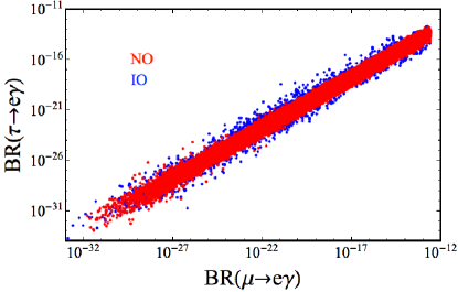
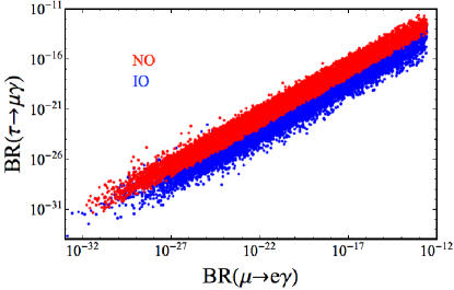
Figure 11: Branching ratios of $\tau\rightarrow e\gamma$ (left panel) and $\tau\rightarrow\mu\gamma$ (right panel) versus that of $\mu\rightarrow e\gamma$ for neutrino masses with normal ordering (in red) and inverted ordering (in blue).

In Fig. 10 we plot the branching ratio of $\mu\rightarrow e\gamma$ versus $|\mathbf{y_{\Phi}}|$ for the same ranges of the quartic coupling $\lambda_{H\Phi\Phi^{\prime}}$ used in Fig. 8 (right panel). The different sets of points form V-shaped regions whose minimum value for $\mathrm{BR}(\mu\to e\gamma)$ is larger the smaller $\lambda_{H\Phi\Phi^{\prime}}$. For $|\mathbf{y_{\Phi}}|\gtrsim 10^{-4}$, the branching ratio scales as $|\mathbf{y_{\Phi}}|^{4}$, independently of $\lambda_{H\Phi\Phi^{\prime}}$. In this region the contribution due to the scalar $\eta^{\prime+}$ is suppressed because $|\mathbf{y_{\Phi^{\prime}}}|\lesssim|\mathbf{y_{\Phi}}|$. If, however, $|\mathbf{y_{\Phi}}|\lesssim 10^{-4}$ the scalar $\eta^{\prime+}$ dominates the branching ratio. The dependence on $\lambda_{H\Phi\Phi^{\prime}}$ again sets the scale of $|\mathbf{y_{\Phi^{\prime}}}|$ and thus the branching ratio of $\mu\rightarrow e\gamma$, i.e., the larger the quartic coupling $\lambda_{H\Phi\Phi^{\prime}}$ the smaller $\text{BR}(\mu\rightarrow e\gamma)$. The minimum value of the branching ratio of these CLFV processes occurs for $|\mathbf{y_{\Phi}}|\sim|\mathbf{y_{\Phi^{\prime}}}|\sim 10^{-4.5}$, when both charged scalar contributions are of similar order, such that the overall result is suppressed.

In Fig. 11 we plot ${\rm BR}(\tau\rightarrow e\gamma)$ (left panel) and ${\rm BR}(\tau\rightarrow\mu\gamma)$ (right panel) versus ${\rm BR}(\mu\rightarrow e\gamma)$, for neutrino masses with NO (in red) and IO (in blue). The central values of these ratios agree with our analytical estimates given in Eqs. (21) and (22), although the entire range of these ratios is about two orders of magnitude. In particular, we see that $\text{BR}(\tau\to e\,\gamma)$ is suppressed compared to $\text{BR}(\tau\to\mu\,\gamma)$ for neutrino masses with NO, while they are very similar for IO. The largest branching ratio is achieved for $\tau\rightarrow\mu\gamma$ for NO, which can be larger than the one for IO. Therefore a measurement could in principle discriminate between the neutrino mass orderings.

4.3.1 Interplay with dark matter direct detection

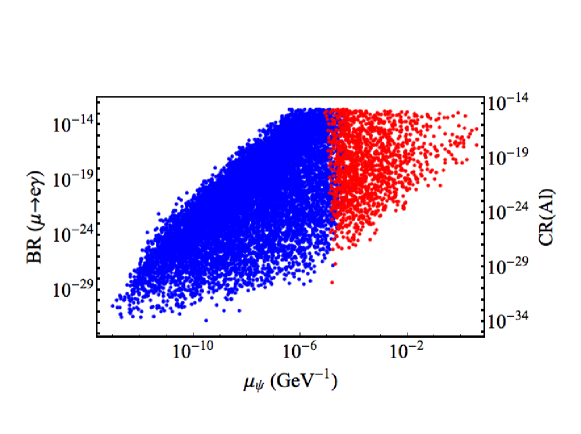
Figure 12: Branching ratio of $\mu\rightarrow e\gamma$ (left axis) and the $\mu-e$ conversion ratio in Al (right axis) versus the dark matter magnetic dipole moment $\mu_{\psi}$ relevant for DM direct detection. We plot in red (blue) the points that are excluded (allowed) by DM direct detection limits.

In Fig. 12 we plot the branching ratio of $\mu\rightarrow e\gamma$ (left axis) and the $\mu-e$ conversion ratio in Al (right axis) versus the DM magnetic dipole moment $\mu_{\psi}$, see Eq. (45), which is relevant for DM direct detection. The size of the magnetic dipole moment $\mu_{\psi}$ is correlated with the branching ratios of CLFV processes, because the structure of the loop diagrams is similar, with a charged scalar in the loop and the same Yukawa couplings. The points in red (blue), corresponding to larger (smaller) values of $\mu_{\psi}$, are excluded (allowed) by the combined constraint from Xenon-based DM direct detection experiments, which are implemented in LikeDM [60]. We can see the interesting complementarity between DM direct detection and CLFV processes in constraining the parameter space of the model. This interplay is further discussed in the generic context for a fermionic SM singlet DM particle in Ref. [50].

5 Variants of the model

5.1 $\rm U(1)_{DM}$ as gauge symmetry

The global $\rm U(1)_{DM}$ symmetry is anomaly-free, because the fermion $\psi$ is vector-like and thus $\rm U(1)_{DM}$ can be straightforwardly gauged. In fact, a similar model with a gauge symmetry has been discussed in Ref. [15]. Three scenarios can be envisaged: $(i)$ $\rm U(1)_{DM}$ is unbroken and the corresponding dark photon $\gamma_{\rm DM}$ is massless, $(ii)$ $\rm U(1)_{DM}$ can be realised non-linearly and the dark photon $\gamma_{\rm DM}$ obtains its mass from the Stückelberg mechanism, or $(iii)$ $\rm U(1)_{DM}$ is spontaneously broken to a residual $Z_{N}$ symmetry, which stabilises the DM candidate. In this case an additional scalar field $\rho$, charged under $\rm U(1)_{\mathrm{DM}}$, has to take a non-vanishing VEV. In case $(i)$ $\gamma_{\rm DM}$ contributes to extra radiation and lead to large self-interactions, see Ref. [80] for a discussion. If in case $(ii)$ and $(iii)$ the mass of the dark photon $\gamma_{\rm DM}$ is smaller than that of the DM candidate, the DM relic abundance is set by annihilations into dark photons. Connections of DM phenomenology to neutrino and flavour physics are then lost so that this case is not interesting to us. In addition, in case $(iii)$ the new scalar field $\rho$ mixes with the SM Higgs doublet $H$. Such mixing is experimentally constrained by invisible Higgs decays, if these are kinematically accessible, and by DM direct detection limits, especially for sub-GeV scalar mediators, thus requiring $\rho$ to be either much heavier than the electroweak scale or the mixing to be small. That in turn is in conflict with the fact that the mediator needs to decay before big bang nucleosynthesis, basically ruling out this possibility [81].

Another effect of gauging $\rm U(1)_{DM}$ is the kinetic mixing with $\rm U(1)_{Y}$, that is the term $\epsilon\,B^{\mu\nu}_{\rm DM}B_{\mu\nu}$ with the field strength tensors $B^{\mu\nu}$ ($B^{\mu\nu}_{\rm DM}$) of $\rm U(1)_{Y}$ ($\rm U(1)_{DM}$). Even if this is tuned to vanish at a certain scale, it arises at one-loop level, since $\Phi$ and $\Phi^{\prime}$ are charged under both $\rm U(1)_{\rm Y}$ and $\rm U(1)_{\rm DM}$. This effect can be estimated as follows: Assuming $\Lambda_{\rm UV}>m_{\Phi},m_{\Phi^{\prime}}>v_{H}$ and a vanishing kinetic mixing at a certain high scale $\Lambda_{\rm UV}$, $\epsilon(\Lambda_{\rm UV})=0$, renormalisation group running can induce a sizeable kinetic mixing at lower scales. Above the mass scales of $\Phi$ and $\Phi^{\prime}$, the opposite values of their hypercharge lead to an exact cancellation of $\epsilon$, but as soon as one of the scalar fields decouples, the kinetic mixing is induced via renormalisation group running, giving the approximate lower bound

$$|\epsilon|\gtrsim\frac{\sqrt{\alpha_{Y}\alpha_{\rm DM}}}{4\pi}\left|\ln\left(\frac{m_{\Phi}}{m_{\Phi^{\prime}}}\right)\right|\,,$$ (48)

with the dark gauge coupling $\alpha_{\rm DM}=g_{\rm DM}^{2}/4\pi$. The annihilation into dark photons is given by $\left\langle v\sigma\right\rangle_{\rm ann}\simeq\pi\alpha_{\rm DM}^{2}/m_{\psi}^{2}$, which implies that in order to reproduce the DM relic abundance $\alpha_{\rm DM}\simeq 10^{-4}\,(m_{\psi}/{\rm GeV})$. Using the experimental value of $\alpha_{Y}(m_{Z})$ [22], and taking the logarithm to be $\mathcal{O}(1)$, we can estimate a lower bound on the kinetic mixing: $|\epsilon|\gtrsim 10^{-4}\,(m_{\psi}/{\rm GeV})$. As in the case of scalar mediators, there are very strong upper limits from DM direct detection, especially if the dark photon is lighter than a few GeV, with only much smaller mixings still allowed, see the recent analysis by the PandaX-II collaboration [81]. In this case, the mediators should decay before big bang nucleosynthesis sets in. Therefore, a certain amount of fine-tuning is required in this case.

5.2 Replacing $\rm U(1)_{DM}$ with $Z_{N}$

Instead of a continuous symmetry we can consider a $Z_{N}$ symmetry, being a subgroup of $\rm U(1)_{DM}$, i.e. we regard the charge of $\Phi$, $\Phi^{\prime}$ and $\psi$ as given modulo $N$.

For $N>4$ the model effectively possesses a global $\rm U(1)$ symmetry, as long as we only consider renormalizable terms in the Lagrangian. Conversely, for $N=2,\,3,$ and $4$, additional terms arise at the renormalizable level.

For $N=2$, i.e. the smallest possible symmetry, we can identify $\psi\leftrightarrow\psi^{c}$ and $\Phi^{\prime}\leftrightarrow\tilde{\Phi}$. The model thus contains one Majorana fermion $\psi$ and one scalar doublet $\Phi$ which are the only particles odd under the $Z_{2}$ symmetry. The Lagrangian for the Majorana fermion $\Psi=\psi+\psi^{c}$ reads

$$\mathcal{L}_{\Psi}\;=\;\frac{1}{2}\left(\overline{\Psi}\,i\,\not{\partial}\,\Psi\,-\,m_{\psi}\,\overline{\Psi}\,\Psi\right)\,-\,\Big{(}y^{\alpha}\,\overline{\Psi}\,{\tilde{\Phi}}^{\dagger}\,L_{\alpha}\,+\,\text{H.c.}\Big{)}\,.$$ (49)

The scalar potential for $\Phi$ and the SM Higgs doublet $H$ becomes

$$\mathcal{V}_{Z_{2}}= \,-\,m_{H}^{2}H^{\dagger}H\,+\,\lambda_{H}(H^{\dagger}H)^{2}\,+\,m_{\Phi}^{2}\Phi^{\dagger}\Phi\,+\,\lambda_{\Phi}(\Phi^{\dagger}\Phi)^{2}\,$$ (50)

$$\,+\,\lambda_{H\Phi}(H^{\dagger}H)(\Phi^{\dagger}\Phi)\,+\,\lambda_{H\Phi,2}(H^{\dagger}\Phi)(\Phi^{\dagger}H)\,+\,\frac{\lambda_{H\Phi,3}}{2}\left[(H^{\dagger}\Phi)^{2}\,+\,{\rm H.c.}\right]\,.$$

The model with a $Z_{2}$ symmetry, a Majorana fermion and one additional scalar doublet has the same symmetries and types of particles as the original ScM, which has been extensively discussed in the literature [3]. We comment on similarities and differences in phenomenology between the latter and the GScM with a global $\rm U(1)$ symmetry in Sec. 6.

For $N=3$ and $N=4$ the Lagrangian ${\cal L}_{\psi}$ remains the same as in Eq. (1), but additional quartic terms appear in the scalar potential, see also Ref. [82]. For $N=3$ there are two new quartic couplings

$$\mathcal{V}_{Z_{3}}=\lambda_{1}\,(\Phi\Phi^{\prime})(H\Phi^{\prime})+\lambda_{2}\,(\Phi\Phi^{\prime})(\tilde{H}\Phi)+{\rm H.c.}$$ (51)

In the case in which one of the new neutral scalars is the lightest particle with non-trivial $Z_{3}$ charge, these terms give rise to DM semi-annihilations [83, 84, 85, 86]. In principle, these new couplings are directly testable at colliders. Furthermore, for $N=4$ the following term can be added to the scalar potential

$$\mathcal{V}_{Z_{4}}=\lambda_{3}\,(\Phi\Phi^{\prime})^{2}+{\rm H.c.}$$ (52)

If one of the new neutral scalars is the lightest particle with non-trivial $Z_{4}$ charge, this term gives rise to DM self-interactions.

5.3 The Generalised Scotogenic Triplet Model

We can construct an interesting variant of the GScM by replacing the fermion singlet with a fermion triplet (we denote it the GScTM). The Lagrangian for the triplet Dirac fermion $\vec{\Sigma}=(\Sigma_{1},\Sigma_{2},\Sigma_{3})$ is

$$\mathcal{L}_{\vec{\Sigma}}\;=\;i\,\overline{\vec{\Sigma}}\,\not{D}\vec{\Sigma}\,-\,m_{\Sigma}\,\overline{\vec{\Sigma}}\vec{\Sigma}\,-\,\Big{[}y_{\Phi}^{\alpha}\,\tilde{\Phi}^{\dagger}\,\left(\overline{\vec{\Sigma}\cdot\vec{\sigma}}\right)\,L_{\alpha}\,+\,\left(y_{\Phi^{\prime}}^{\alpha}\right)^{*}\,\tilde{\Phi}^{\prime\dagger}\,\left(\overline{\vec{\Sigma}\cdot\vec{\sigma}}\right)\,\tilde{L}_{\alpha}\,+\,\text{H.c.}\Big{]}\,,$$ (53)

where $\vec{\sigma}=(\sigma_{1},\sigma_{2},\sigma_{3})$ and the covariant derivative for the electroweak triplet fermion, $D_{\mu}=\partial_{\mu}+ig\tau_{3}^{a}W_{\mu}^{a}$, with the three generators $\tau_{3}^{a}$ of the triplet representation. The three physical Dirac fermion fields are as usual $\Sigma_{0}=\Sigma_{3}$ and $\Sigma_{\pm}=\frac{1}{\sqrt{2}}(\Sigma_{1}\mp\Sigma_{2})$, which are degenerate in mass at tree level. Radiative corrections lift the charged components by 166 MeV [87, 88]. Notice that due to the dark symmetry the components of the fermion triplet do not mix with SM leptons.

As we saw, in the case of GScM with singlet fermionic DM, the relic abundance cannot be explained by annihilations due to the strong limits from CLFV. In the case of the GScTM with triplet fermionic DM (we take its mass to be smaller than the scalars mass), the phenomenology is very different. The relic abundance, driven by gauge interactions, is decoupled from the neutrino and LFV phenomenology. This implies that the coannihilations of the GScM with the scalars, which involve some degree of fine tuning, are not needed. The dominant annihilation channels of the triplets are through gauge interactions, like $\Sigma_{0}\Sigma_{0}\rightarrow W^{+}W^{-}$, mediated by the charged scalar $\Sigma_{+}$. Due to the small splitting between the neutral and the charged components, there are also important contributions from coannihilation channels like $\Sigma_{0}\Sigma_{+}\rightarrow Z/\gamma/H+W^{+}$ mediated by the charged $\Sigma_{+}$ (t-channel) or by a $W^{+}$ (s-channel), and $\Sigma_{0}\Sigma_{+}\rightarrow f\bar{f}$, mediated also by a $W^{+}$ (s-channel), where f are SM fermions. In this case reproducing the relic abundance fixes the mass of the fermion triplet to be equal to $2.7$ TeV [89].

Regarding direct detection, the Z does not couple to the neutral fermion, so there is no tree level scattering. Moreover, the splitting with the charged fermion (166 MeV) being larger than the typical recoil momentum in direct detection experiments makes it impossible to have inelastic scattering mediated by a W. There are extra one-loop penguin diagrams in addition to those present for a fermion singlet, with the photon/H/Z attached to the $W^{+}$ in the loop, and with the photon/Z attached to the $\Sigma_{+}$ in the loop, as well as box diagrams with W in the loop, see Refs. [90, 91, 88].

The presence of charged fermion components generate also extra contributions to CLFV, as well as new collider signatures, similar to the wino in SUSY. However the large triplet mass makes its production at the LHC very suppressed, being necessary a future collider to probe directly the model. The new charged fermions or scalars can be pair produced at colliders via the Drell-Yan process with a photon or $Z$ boson. Another important production channel is $\overline{u}d\rightarrow W^{-}\rightarrow\Sigma_{-}\Sigma_{0}$. The interesting feature is that the lifetime of the $\Sigma_{+}$ is fixed, such that it generates charged tracks at colliders of length equal to $5.5$ cm. The charged fermions $\Sigma_{+}$ will decay into the DM (MET) $\Sigma_{0}$ plus a very soft W, which in turn decays into pions and leptons with the branching ratios [88]: ${\rm BR}(\Sigma_{+}\rightarrow\Sigma_{0}\pi^{+})=0.977$, ${\rm BR}(\Sigma_{+}\rightarrow\Sigma_{0}e^{+}\nu_{e})=0.0205$, ${\rm BR}(\Sigma_{+}\rightarrow\Sigma_{0}\mu^{+}\nu_{\mu})=0.0025$. One can also produce the scalars via $\overline{u}d\rightarrow W^{-}\rightarrow\eta^{+}\eta^{0}$, which decay into $\Sigma_{0}+\ell^{+}$ or $\Sigma_{+}+\nu_{\ell}$, with $\ell=e,\mu,\tau$. These last decays involve the neutrino Yukawas, and therefore there are definite predictions for the ratios of lepton flavours. Other collider studies of the fermion triplet in the context of seesaw type III have been performed in Refs. [92, 93].

6 Comparison with the Scotogenic Model

As already mentioned in Sec. 5, if the global $\rm U(1)_{DM}$ symmetry is replaced by a $Z_{2}$ symmetry, the GScM coincides in symmetries and types of particles with the original ScM [3]. In the following, we highlight similarities and differences between the latter and the GScM discussed here.

In order to generate at least two neutrino masses, at least two Majorana fermions $\psi_{1,2}$ (with masses $m_{\psi_{1,2}}$) and one additional inert scalar doublet field are needed in the ScM, whereas in the GScM one Dirac fermion and two new scalar doublet fields are needed. We have thus one more charged and one more neutral complex scalar filed in the GScM compared to the ScM. In the latter model the scalar mass spectrum, derived from the potential in Eq. (50), reads

$$m_{\phi_{0}^{R}} = \sqrt{m_{\Phi}^{2}\,+\,\frac{1}{2}\left(\lambda_{H\Phi}\,+\,\lambda_{H\Phi,2}\,+\,\lambda_{H\Phi,3}\right)v_{H}^{2}}\,,$$ (54)

$$m_{\phi_{0}^{I}} = \sqrt{m_{\Phi}^{2}\,+\,\frac{1}{2}\left(\lambda_{H\Phi}\,+\,\lambda_{H\Phi,2}\,-\,\lambda_{H\Phi,3}\right)v_{H}^{2}}\,,$$ (55)

$$m_{\phi^{+}} = \sqrt{m_{\Phi}^{2}\,+\,\frac{1}{2}\lambda_{H\Phi}\,v_{H}^{2}}$$ (56)

with $\phi_{0}^{R}$ and $\phi_{0}^{I}$ being the real and imaginary components of the neutral component $\phi_{0}$ of the additional scalar doublet, $\phi_{0}\equiv(\phi_{0}^{R}\,+\,i\,\phi_{0}^{I})/\sqrt{2}$, and $\phi^{+}$ the charged component of the scalar doublet. The scalars $\phi_{0}^{R}$ and $\phi_{0}^{I}$ acquire a mass splitting proportional to the quartic coupling $\lambda_{H\Phi,3}$. In contrast, in the GScM the mass spectrum, given in Eq. (9), clearly shows that real and imaginary parts of the neutral scalars have the same mass and form complex neutral scalars, denoted $\eta_{0}$ and $\eta_{0}^{\prime}$.

In the ScM neutrino masses are generated by diagrams with the neutral scalars $\phi_{0}^{R}$ and $\phi_{0}^{I}$ running in the loop. The neutrino mass matrix is given by

$$\left(\mathcal{M}_{\nu}\right)_{\alpha\beta} = \,\sum_{k}\,\frac{y_{\alpha k}\,y_{\beta k}\,m_{\psi_{k}}}{32\,\pi^{2}}\,\,F(m_{\phi_{0}^{R}},m_{\phi_{0}^{I}},m_{\psi_{k}})\,,$$ (57)

where the loop function is defined in Eq. (13). We can see how the difference in mass between the two complex neutral scalars $\eta_{0}$ and $\eta_{0}^{\prime}$ in the GScM, that appears in neutrino masses, see Eq. (12), is traded for the difference in mass between the neutral scalars $\phi_{0}^{R}$ and $\phi_{0}^{I}$ in the ScM. As is well-known, in the ScM lepton number is broken by the simultaneous presence of the Yukawa couplings, the masses of the Majorana fermions $\psi_{k}$ and the quartic coupling $\lambda_{H\Phi,3}$ of the potential in Eq. (50). Thus neutrino masses crucially depend on all three of them. While the dependence on the first two ones is obvious from Eq. (57), the one on $\lambda_{H\Phi,3}$ is best revealed in the limit $m_{\phi_{0}^{R}}^{2}-m_{\phi_{0}^{I}}^{2}=\lambda_{H\Phi,3}v_{H}^{2}\ll m_{0}^{2}\equiv(m_{\phi_{0}^{R}}^{2}+m_{\phi_{0}^{I}}^{2})/2$ where the expression for the neutrino mass matrix takes the form

$$\left(\mathcal{M}_{\nu}\right)_{\alpha\beta}=\frac{\lambda_{H\Phi,3}v_{H}^{2}}{32\,\pi^{2}}\sum_{k}\frac{y_{\alpha k}\,y_{\beta k}\,m_{\psi_{k}}}{m_{0}^{2}-m_{\psi_{k}}^{2}}\left[1-\cfrac{m_{\psi_{k}}^{2}}{m_{0}^{2}-m_{\psi_{k}}^{2}}\ln\cfrac{m_{0}^{2}}{m_{\psi_{k}}^{2}}\right]\,.$$ (58)

This is similar to what happens in the GScM, where the simultaneous presence of both Yukawa couplings $y^{\alpha}_{\Phi}$ and $y^{\alpha}_{\Phi^{\prime}}$, the fermion mass $m_{\psi}$ and the quartic coupling $\lambda_{H\Phi\Phi^{\prime}}$ is required in order to break lepton number. Consequently, neutrino masses are proportional to all these quantities, as can be read off from Eq. (12) together with Eqs. (7) and (9).

In the original ScM CLFV processes have been studied in detail in Refs. [3, 5] (see also Ref. [42]). It turns out that the individual penguin diagram contributions of a charged scalar and a fermion to CLFV processes in the original ScM are the same as the ones in the GScM, see Sec. 3. However, the number of charged scalars and fermions differs in the two models. We therefore obtain a different number of contributions to CLFV processes in the two models. Moreover, there are new box diagrams for trilepton decays in the GScM.

The DM phenomenology is different in the original ScM and in the GScM. For scalar DM the main channels for DM direct detection in the former are the tree-level mediated processes by the $Z$ and the Higgs boson [94]. For $\lambda_{H\Phi,3}\neq 0$ the scalar ($\phi_{0}^{R}$) and pseudoscalar ($\phi_{0}^{I}$) have different masses and DM scattering off nuclei is an inelastic process, with the $Z$-boson exchange typically dominating. This imposes a lower bound on $\lambda_{H\Phi,3}$ in order to kinematically forbid such scattering. In the GScM scalar DM, with $\eta_{0}^{\prime}$ being the DM particle, also naturally has a large DM direct detection cross section mediated by the $Z$ boson, unless the interaction with the $Z$ boson is suppressed, like for maximal mixing $\theta=\pi/4$. Moreover, there is an elastic contribution via Higgs-boson exchange.

For fermionic DM in the ScM DM-nucleon scattering occurs at one-loop level [9] via penguin diagrams, which happens similarly in the GScM, see Sec. 3.6. If the mass splitting between the Majorana fermions $\psi_{k}$ is sufficiently small, there is a transitional magnetic dipole moment interaction with charged leptons running in the loop. This leads to inelastic DM-nucleon scattering. As discussed in Sec. 3.6, in the GScM the dominant DM-nucleon scattering occurs via a magnetic dipole moment interaction with charged leptons running in the loop.

7 Summary and conclusions

We have studied a model in which masses for neutrinos are generated at one-loop level with Dirac fermion DM running in the loop. The model can be viewed as a generalised version of the ScM (GScM) with a global U(1)_DM symmetry. Both neutrino mass orderings (NO and IO) can be accommodated. The flavour structure of the neutrino Yukawa couplings is determined by the neutrino oscillation parameters and the Majorana phase $\gamma$. The model is has some definite predictions. The flavour structure relevant for neutrino masses differs from the one appearing in the expressions for the branching ratios of CLFV processes, in contrast to the original ScM. We have obtained interesting correlations among the ratios of different CLFV processes, which may allow to test the GScM and to discriminate between the two neutrino mass orderings.

In this work we have focused on fermionic DM, given the fact that scalar DM would require some fine-tuning. The main DM annihilation channels are into charged leptons and neutrinos. As they depend on the same Yukawa couplings relevant for CLFV processes, the corresponding cross sections are too small in order to explain the observed DM relic density and thus coannihilations are important. In roughly half of the parameter space of the model, the next-to-lightest particle is the lightest neutral scalar ($\eta_{0}^{\prime}$), and in the other half it is the lightest charged scalar (which can be either $\eta^{\pm}$ or $\eta^{\prime\pm}$).

Experimental limits on the branching ratios of CLFV processes and on DM direct detection give complementary information on the parameter space of the model. Future experiments, searching for $\mu-e$ conversion in nuclei and $\mu\rightarrow 3e$, will probe the remaining allowed parameter space of the model best, but also DM direct detection experiments will further test a complementary region of the available parameter space of the model. Another interesting signature of the model is the production of new (neutral and charged) scalars at colliders and the decay of the charged scalars to a charged lepton and DM. For neutrino masses with NO the dominant channels are into muons and $\tau$ leptons, while for neutrino masses with IO the decay into electrons is of similar magnitude.

In comparison to the original ScM, the GScM has more degrees of freedom in the scalar sector (two additional doublets versus one in the ScM), and possesses one vector-like Dirac fermion, unlike the ScM which contains at least two Majorana fermions. The flavour structure in the GScM is more restricted by the neutrino oscillation parameters than in the original ScM with three Majorana fermions. Nonetheless, they both are simple explanations for neutrino masses and DM with a rich and testable phenomenology.

Appendix A Stability of the potential

We follow closely the vacuum stability conditions derived from co-positivity criteria in Refs. [95, 96]. For large field values only the quartic part ${\cal V}_{4}$ of the potential is relevant. Using the following parametrisation

$$H^{\dagger}H=h_{1}^{2},\qquad\qquad\qquad\Phi^{\dagger}\Phi=h_{2}^{2},\qquad\qquad\qquad\Phi^{\prime\dagger}\Phi^{\prime}=h_{3}^{2},$$ (59)

$${H^{\dagger}}\Phi=h_{1}h_{2}\rho_{12}e^{i\phi_{12}},\;\;\;\;\;\;{H^{\dagger}}\tilde{\Phi}^{\prime}=h_{1}h_{3}\rho_{13}e^{i\phi_{13}},\;\;\;\;\;\;{\Phi^{\dagger}}\tilde{\Phi}^{\prime}=h_{2}h_{3}\rho_{23}e^{i\phi_{23}}\;,$$

with $0\leq\rho_{ij}\leq 1$ and $0\leq\phi_{ij}\leq 2\,\pi$, ${\cal V}_{4}$ reads

$${\cal V}_{4}= \,\lambda_{H}\,h_{1}^{4}\,+\,\lambda_{\Phi}\,h_{2}^{4}\,+\,\lambda_{\Phi^{\prime}}\,h_{3}^{4}\,+\,\left(\lambda_{H\Phi}\,+\,\lambda_{H\Phi,2}\,\rho_{12}^{2}\right)\,h_{1}^{2}\,h_{2}^{2}$$ (60)

$$\,+\,\left(\lambda_{H\Phi^{\prime}}\,+\,\lambda_{H\Phi^{\prime},2}\,\rho_{13}^{2}\right)\,h_{1}^{2}\,h_{3}^{2}\,+\,\left(\lambda_{\Phi\Phi^{\prime}}\,+\,\lambda_{\Phi\Phi^{\prime},2}\,\rho_{23}^{2}\right)\,h_{2}^{2}\,h_{3}^{2}$$

$$\,+\,2\,\lambda_{H\Phi\Phi^{\prime}}\,h_{1}^{2}\,h_{2}\,h_{3}\,\rho_{12}\,\rho_{13}\,\cos(\phi_{12}+\phi_{13})\,.$$

If we neglect $\lambda_{H\Phi\Phi^{\prime}}$, we can write ${\cal V}_{4}$ as a bilinear form

$${\cal V}_{4} =\left(\begin{array}[]{ccc}h_{1}^{2}&h_{2}^{2}&h_{3}^{2}\end{array}\right)\,Q\,\left(\begin{array}[]{c}h_{1}^{2}\\ h_{2}^{2}\\ h_{3}^{2}\end{array}\right)$$ (65)

with

$$Q \equiv\left(\begin{array}[]{ccc}\lambda_{H}&\frac{1}{2}\,(\lambda_{H\Phi}+\lambda_{H\Phi,2}\,\rho_{12}^{2})&\frac{1}{2}\,(\lambda_{H\Phi^{\prime}}+\lambda_{H\Phi^{\prime},2}\,\rho_{13}^{2})\\ \frac{1}{2}\,(\lambda_{H\Phi}+\lambda_{H\Phi,2}\,\rho_{12}^{2})&\lambda_{\Phi}&\frac{1}{2}\,(\lambda_{\Phi\Phi^{\prime}}+\lambda_{\Phi\Phi^{\prime},2}\,\rho_{23}^{2})\\ \frac{1}{2}\,(\lambda_{H\Phi^{\prime}}+\lambda_{H\Phi^{\prime},2}\,\rho_{13}^{2})&\frac{1}{2}\,(\lambda_{\Phi\Phi^{\prime}}+\lambda_{\Phi\Phi^{\prime},2}\,\rho_{23}^{2})&\lambda_{\Phi^{\prime}}\end{array}\right)$$ (69)

and determine the necessary conditions for the stability of the potential. We find

$$\lambda_{H}\geq 0\;,\;\;\lambda_{\Phi}\geq 0\;,\;\;\lambda_{\Phi^{\prime}}\geq 0$$ (70)

and

$$c_{1}=\frac{1}{2}\,(\lambda_{H\Phi}+\lambda_{H\Phi,2}\,\rho_{12}^{2})+\sqrt{\lambda_{H}\,\lambda_{\Phi}}\geq 0\;,$$ (71)

$$c_{2}=\frac{1}{2}\,(\lambda_{H\Phi^{\prime}}+\lambda_{H\Phi^{\prime},2}\,\rho_{13}^{2})+\sqrt{\lambda_{H}\,\lambda_{\Phi^{\prime}}}\geq 0\;,$$

$$c_{3}=\frac{1}{2}\,(\lambda_{\Phi\Phi^{\prime}}+\lambda_{\Phi\Phi^{\prime},2}\,\rho_{23}^{2})+\sqrt{\lambda_{\Phi}\,\lambda_{\Phi^{\prime}}}\geq 0\;,$$

together with

$$\sqrt{\lambda_{H}\,\lambda_{\Phi}\,\lambda_{\Phi^{\prime}}}+\frac{1}{2}\,(\lambda_{H\Phi}+\lambda_{H\Phi,2}\,\rho_{12}^{2})\sqrt{\lambda_{\Phi^{\prime}}}+\frac{1}{2}\,(\lambda_{H\Phi^{\prime}}+\lambda_{H\Phi^{\prime},2}\,\rho_{13}^{2})\sqrt{\lambda_{\Phi}}$$ (72)

$$\phantom{xxxxxxxxxxxxxxxxxxxxxxx}+\frac{1}{2}\,(\lambda_{\Phi\Phi^{\prime}}+\lambda_{\Phi\Phi^{\prime},2}\,\rho_{23}^{2})\sqrt{\lambda_{H}}+\sqrt{2\,c_{1}\,c_{2}\,c_{3}}\geq 0\;.$$

Depending on the sign of $\lambda_{H\Phi,2}$, $\lambda_{H\Phi^{\prime},2}$ and $\lambda_{\Phi\Phi^{\prime},2}$ the necessary conditions are given for $\rho_{ij}=0$ or $\rho_{ij}=1$, i.e. for $\lambda_{H\Phi,2}>0$ the necessary conditions are obtained for $\rho_{12}=0$, while for $\lambda_{H\Phi,2}<0$ these are given for $\rho_{12}=1$. The same is true for $\lambda_{H\Phi^{\prime},2}$ and $\rho_{13}$ as well as for $\lambda_{\Phi\Phi^{\prime},2}$ and $\rho_{23}$.

For non-zero $\lambda_{H\Phi\Phi^{\prime}}$ we derive sufficient (but not necessary) conditions for the stability of the potential from considering co-positivity. We re-write ${\cal V}_{4}$ as

$${\cal V}_{4} = h_{1}^{4}\,\left[\lambda_{H}+\left(\begin{array}[]{cc}\tilde{h}_{2}^{2}&\tilde{h}_{3}^{2}\end{array}\right)\,\left(\begin{array}[]{cc}\lambda_{\Phi}&\frac{1}{2}\,(\lambda_{\Phi\Phi^{\prime}}+\lambda_{\Phi\Phi^{\prime},2}\,\rho_{23}^{2})\\ \frac{1}{2}\,(\lambda_{\Phi\Phi^{\prime}}+\lambda_{\Phi\Phi^{\prime},2}\,\rho_{23}^{2})&\lambda_{\Phi^{\prime}}\end{array}\right)\,\left(\begin{array}[]{c}\tilde{h}_{2}^{2}\\ \tilde{h}_{3}^{2}\end{array}\right)\right.$$ (84)

$$\left.+\,\left(\begin{array}[]{cc}\tilde{h}_{2}&\tilde{h}_{3}\end{array}\right)\,\left(\begin{array}[]{cc}\lambda_{H\Phi}+\lambda_{H\Phi,2}\,\rho_{12}^{2}&\lambda_{H\Phi\Phi^{\prime}}\,\rho_{12}\,\rho_{13}\,\cos(\phi_{12}+\phi_{13})\\ \lambda_{H\Phi\Phi^{\prime}}\,\rho_{12}\,\rho_{13}\,\cos(\phi_{12}+\phi_{13})&\lambda_{H\Phi^{\prime}}+\lambda_{H\Phi^{\prime},2}\,\rho_{13}^{2}\end{array}\right)\,\left(\begin{array}[]{c}\tilde{h}_{2}\\ \tilde{h}_{3}\end{array}\right)\right]$$

with $\tilde{h}_{2,3}$ being $h_{2,3}$ rescaled by $h_{1}$. We require then co-positivity of the three different terms of ${\cal V}_{4}$. This leads to

$$\lambda_{H}\geq 0$$ (85)

and to

$$\lambda_{\Phi}\geq 0\;\;,\;\;\lambda_{\Phi^{\prime}}\geq 0\;\;\;\mbox{and}\;\;\;\frac{1}{2}(\lambda_{\Phi\Phi^{\prime}}+\lambda_{\Phi\Phi^{\prime},2}\,\rho_{23}^{2})+\sqrt{\lambda_{\Phi}\,\lambda_{\Phi^{\prime}}}\geq 0\,,$$ (86)

with the last condition depending on the sign of $\lambda_{\Phi\Phi^{\prime},2}$, i.e. $\rho_{23}=0\,(1)$ for positive (negative) $\lambda_{\Phi\Phi^{\prime},2}$. In order to use co-positivity of the last term we first minimise ${\cal V}_{4}$ with respect to $\rho_{12}$, $\rho_{13}$ and $\cos(\phi_{12}+\phi_{13})$. The term with $\lambda_{H\Phi\Phi^{\prime}}$ alone is minimised for $\cos(\phi_{12}+\phi_{13})=-1$. From the extreme values of $\rho_{12}$ and $\rho_{13}$ that minimise ${\cal V}_{4}$ we derive then the sufficient conditions

$$\lambda_{H\Phi}\geq 0\;\;,\;\;\lambda_{H\Phi^{\prime}}\geq 0\;\;,\;\;\lambda_{H\Phi}+\lambda_{H\Phi,2}\geq 0\;\;,\;\;\lambda_{H\Phi^{\prime}}+\lambda_{H\Phi^{\prime},2}\geq 0\;\;,$$ (87)

$$\mbox{and}\;\;\;\sqrt{(\lambda_{H\Phi}+\lambda_{H\Phi,2})(\lambda_{H\Phi^{\prime}}+\lambda_{H\Phi^{\prime},2})}-\lambda_{H\Phi\Phi^{\prime}}\geq 0\;.$$

Only the last condition involves $\lambda_{H\Phi\Phi^{\prime}}$ and bounds the latter from above.

${\cal V}_{4}$ is also minimised for non-extremal values of $\rho_{12}$ and $\rho_{13}$. This, however, does not imply conditions different from those already shown above, but only leads to an equality involving $\lambda_{H\Phi\Phi^{\prime}}$, $\lambda_{H\Phi,2}$ and $\lambda_{H\Phi^{\prime},2}$ which needs to be fulfilled in addition. We have checked that the presented conditions can also be applied to the special directions in which one or two of $h_{1,2,3}$ vanish.

Appendix B Neutrino masses and lepton mixing

We can diagonalize the neutrino mass matrix in Eq. (12) as

$$\mathcal{M}_{\nu}=U^{*}D_{\nu}U^{\dagger}\,,$$ (88)

where $D_{\nu}$ is a $3\times 3$ diagonal matrix with positive semi-definite eigenvalues (in our model with $m_{1}=0$ for NO, and $m_{3}=0$ for IO). $U$ is the PMNS mixing matrix, which relates the neutrino mass eigenstates $\nu_{i}$ ($i=1,2,3$) with masses $m_{i}$ to the neutrino flavour eigenstates $\nu_{\alpha}$ ($\alpha=e,\mu,\tau$):

$$\nu_{\alpha}=\sum_{i=1}^{3}\,U^{*}_{i\alpha}\,\nu_{i}\,.$$ (89)

The standard parametrisation for $U$ for one massless neutrino is

$$U=\left(\begin{array}[]{ccc}c_{13}c_{12}&c_{13}s_{12}&s_{13}e^{-i\delta}\\ -c_{23}s_{12}-s_{23}s_{13}c_{12}e^{i\delta}&c_{23}c_{12}-s_{23}s_{13}s_{12}e^{i\delta}&s_{23}c_{13}\\ s_{23}s_{12}-c_{23}s_{13}c_{12}e^{i\delta}&-s_{23}c_{12}-c_{23}s_{13}s_{12}e^{i\delta}&c_{23}c_{13}\end{array}\right)\left(\begin{array}[]{ccc}1&0&0\\ 0&e^{i\gamma}&0\\ 0&0&1\end{array}\right)\,,$$ (96)

where $c_{ij}\equiv\cos\theta_{ij}$ and $s_{ij}\equiv\sin\theta_{ij}$ ($\theta_{12}$, $\theta_{13}$, and $\theta_{23}$ being the three lepton mixing angles). $\gamma$ is the Majorana and $\delta$ the Dirac phase. Since the lightest neutrino is massless in the GScM, there is only one physical Majorana phase.

Appendix C Parametrisation of the neutrino Yukawa couplings

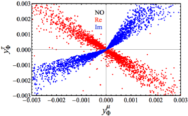
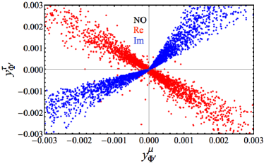
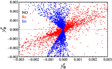
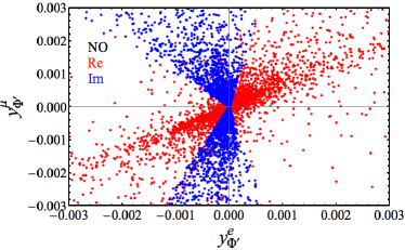
Figure 13: Neutrino Yukawa couplings $y_{\Phi}^{\alpha}$ (left panels) and $y_{\Phi^{\prime}}^{\alpha}$ (right panels) for neutrino masses with normal ordering, separated according to real (in red) and imaginary parts (in blue). The upper panel shows the flavour $\tau$ versus $\mu$, while the lower one shows $\mu$ versus $e$.

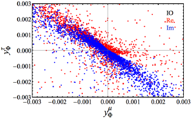
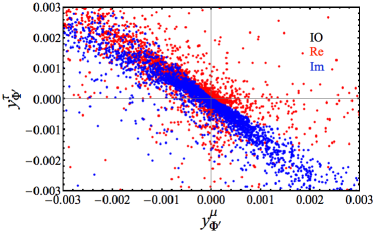
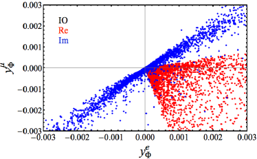
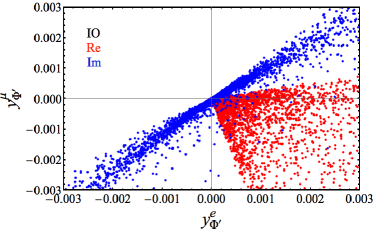
Figure 14: The same as in Fig. 13 for neutrino masses with inverted ordering.

We want to express the neutrino Yukawa couplings in terms of neutrino masses and lepton mixing parameters. We follow the discussion in Ref. [97]. On the one hand, the rank-two neutrino mass matrix can be expressed in terms of the two non-vanishing mass eigenvalues and two columns of the PMNS mixing matrix, $u_{i}$, in the flavour basis

$${\cal M}_{\nu}=\sum_{i}m_{i}u_{i}^{*}u_{i}^{\dagger}=\sum_{i}v_{i}v_{i}^{T}\;.$$ (97)

The vectors $v_{i}\equiv\sqrt{m_{i}}u_{i}^{*}$ are linearly independent and span a two-dimensional vector space. On the other hand, the calculation of the neutrino mass matrix results in the following form

$${\cal M}_{\nu}=x_{1}x_{2}^{T}+x_{2}x_{1}^{T}$$ (98)

with

$$x_{1}=\,\sqrt{\frac{\sin 2\theta\,m_{\psi}}{32\,\pi^{2}}\,F(m_{\eta_{0}},m_{\eta_{0}^{\prime}},m_{\psi})}\,y_{\Phi}\;,\;x_{2}=\,\sqrt{\frac{\sin 2\theta\,m_{\psi}}{32\,\pi^{2}}\,F(m_{\eta_{0}},m_{\eta_{0}^{\prime}},m_{\psi})}\,y_{\Phi^{\prime}}\,,$$ (99)

see Eqs. (12) and (13). If $\sin 2\theta<0$ the square roots yield a complex number. The two linearly independent vectors $x_{i}$ can be written in terms of the vectors $v_{i}$

$$x_{i}=a_{ij}v_{j}\,,$$ (100)

where $(a_{ij})$ forms an invertible $2\times 2$ matrix, i.e. $\det a=a_{11}a_{22}-a_{12}a_{21}\neq 0$. Using the two different parametrisations of the neutrino mass matrix, we can find possible solutions of $a_{ij}$

$${\cal M}_{\nu} =x_{1}x_{2}^{T}+x_{2}x_{1}^{T}$$ (101)

$$=\sum_{i,j}a_{1i}a_{2j}v_{i}v_{j}^{T}+\sum_{i,j}a_{2i}a_{1j}v_{i}v_{j}^{T}=\sum_{i,j}(a_{1i}a_{2j}+a_{2i}a_{1j})v_{i}v_{j}^{T}$$ (102)

$$=\sum_{i}v_{i}v_{i}^{T}\,.$$ (103)

As the vectors $v_{i}$ form a basis of the two-dimensional vector space, we find

$$a_{11}a_{21}+a_{21}a_{11} =1 \Rightarrow\quad a_{11}a_{21} =\frac{1}{2}\,,$$ (104)

$$a_{12}a_{22}+a_{22}a_{12} =1 \Rightarrow\quad a_{12}a_{22} =\frac{1}{2}\,,$$ (105)

$$a_{11}a_{22}+a_{21}a_{12} =0 \Rightarrow\quad a_{11}^{2}a_{22}^{2} =a_{12}^{2}a_{21}^{2}=-\frac{1}{4}\,.$$ (106)

In particular the matrix elements are non-zero, $a_{ij}\neq 0$. There are two sets of solutions. Writing the complex matrix element $a_{11}=re^{i\alpha}$ in terms of two real parameters $r,\,\alpha$ we obtain

$$a_{11} =re^{i\alpha}\,\equiv\frac{\zeta}{\sqrt{2}}, a_{21} =\frac{1}{2r}e^{-i\alpha}\,, a_{22} =\frac{1}{2r}e^{-i\left(\alpha\pm\frac{\pi}{2}\right)}\,, a_{12} =re^{i\left(\alpha\pm\frac{\pi}{2}\right)}$$ (107)

and the condition of a non-vanishing determinant

$$0\neq\det a=a_{11}a_{22}-a_{12}a_{21}=2\,a_{11}a_{22}=e^{\mp i\frac{\pi}{2}}$$ (108)

is trivially satisfied for the two solutions. Thus the two vectors can be uniquely written as

$$x_{1} =\frac{\zeta}{\sqrt{2}}\left(v_{1}\pm iv_{2}\right),\, x_{2} =\frac{1}{\sqrt{2}\zeta}\left(v_{1}\mp iv_{2}\right)\,.$$ (109)

For NO we obtain

$$x_{1}^{\mathrm{(NO)}}=\frac{\zeta}{\sqrt{2}}\left(\sqrt{m_{2}}u_{2}^{*}\pm i\sqrt{m_{3}}u_{3}^{*}\right),\,\qquad\,x_{2}^{\mathrm{(NO)}}=\frac{1}{\sqrt{2}\zeta}\left(\sqrt{m_{2}}u_{2}^{*}\mp i\sqrt{m_{3}}u_{3}^{*}\right),\,$$ (110)

while for IO, we have that

$$x_{1}^{\mathrm{(IO)}}=\frac{\zeta}{\sqrt{2}}\left(\sqrt{m_{1}}u_{1}^{*}\pm i\sqrt{m_{2}}u_{2}^{*}\right),\,\qquad\,x_{2}^{\mathrm{(IO)}}=\frac{1}{\sqrt{2}\zeta}\left(\sqrt{m_{1}}u_{1}^{*}\mp i\sqrt{m_{2}}u_{2}^{*}\right)\,.$$ (111)

Without loss of generality we choose $\zeta$ to be real and positive. Any phase of $\zeta$ can be absorbed via phase redefinitions of the lepton doublets $L_{\alpha}$ and the Dirac fermion $\psi$. In Figs. 13 and 14 we show the results for $y_{\Phi}^{\alpha}$ (left) and $y_{\Phi^{\prime}}^{\alpha}$ (right) for neutrino masses with NO and IO, respectively, separated according to real (in red) and imaginary (in blue) parts, as obtained in the numerical scans. We show different flavours: the upper panel shows the flavour $\tau$ versus $\mu$, while the lower one shows $\mu$ versus $e$. We clearly see that $y_{\Phi}^{\alpha}$ and $y_{\Phi^{\prime}}^{\alpha}$ of different flavour $\alpha$ are correlated. These correlations can be understood analytically to a certain extent, see Sec. 2.2.

Appendix D Loop functions

In this appendix we collect loop functions and other inputs appearing in CLFV processes, $h\rightarrow\gamma\gamma$ and DM direct detection.

The loop functions for the dipole and monopole photon contributions to CLFV processes are

$$\begin{split}f(x)\;=\;&\frac{1-6x+3x^{2}+2x^{3}-6x^{2}\ln(x)}{6(1-x)^{4}}\,,\\ g(x)\;=\;&\frac{2-9x+18x^{2}-11x^{3}+6x^{3}\ln(x)}{12(1-x)^{4}}\,.\end{split}$$ (112)

The following ones enter in the box diagrams of trilepton decays

$$\begin{split}h_{1}(x)\;=\;&\frac{1-x^{2}+2x\ln x}{2(x-1)^{3}}\,,\\ h_{2}(x,y)\;=\;&-\frac{xy}{2(1-x)(1-y)}-\frac{x^{2}y\ln x}{2(1-x)^{2}(x-y)}-\frac{xy^{2}\ln y}{2(1-y)^{2}(y-x)}\,.\end{split}$$ (113)

The numerical values of the overlap integrals $D$ and $V^{(p,n)}$ and the total muon capture rate $\omega_{\mathrm{capt}}$, needed for the computation of $\mu-e$ conversion ratios in nuclei, are shown in Tab. 5 for three different nuclei.

	$V^{(p)}$	$V^{(n)}$	$D$	$\omega_{\rm capt}(10^{6}\text{s}^{-1})$
${}^{197}_{79}\text{Au}$	0.0859	0.108	0.167	13.07
${}^{48}_{22}\text{Ti}$	0.0399	0.0495	0.0870	2.59
${}^{27}_{13}\text{Al}$	0.0159	0.0169	0.0357	0.7054

Table 5: Overlap integrals in units of $m_{\mu}^{5/2}$ ($V^{(p)}$, $V^{(n)}$ and $D$) and total capture rates ($\omega_{\rm capt}$) for different nuclei [30]. The total capture rates are taken from Tab. 8 in Ref. [30]. The overlap integrals of ${}^{197}_{79}\text{Au}$ as well as ${}^{27}_{13}\text{Al}$ are taken from Tab. 2 and the ones for ${}^{48}_{22}\text{Ti}$ are taken from Tab. 4 in Ref. [30].

The relevant loop function for the DM magnetic dipole moment which gives the dominant contribution to DM direct detection is

$$f_{\rm DD}(x,y,z) =1-\frac{y^{2}-z^{2}}{x^{2}}\ln\frac{y}{x}$$

$$+\frac{y^{4}+z^{4}-x^{2}y^{2}-x^{2}z^{2}-2z^{2}y^{2}}{x^{2}\lambda^{1/2}(z^{2},x^{2},y^{2})}\,\ln\frac{y^{2}-x^{2}+z^{2}+\lambda^{1/2}(z^{2},x^{2},y^{2})}{2yz}$$ (114)

with the Källén-$\lambda$ function $\lambda(x,y,z)=x^{2}+y^{2}+z^{2}-2xy-2yz-2zx$.

In $h\rightarrow\gamma\gamma$ we need the following loop functions for scalars, fermions and gauge bosons $A_{i}(x)$ $(i=0,1/2,1)$

$$A_{0}(x) =-x+x^{2}\,f\left(\frac{1}{x}\right)\,,$$ (115)

$$A_{1/2}(x) =2x+2x(1-x)\,f\left(\frac{1}{x}\right)\,,$$ (116)

$$A_{1}(x) =-2-3x-3x(2-x)\,f\left(\frac{1}{x}\right)\,.$$ (117)

Appendix E Oblique parameters

The two inert scalar doublets $\Phi$ and $\Phi^{\prime}$ contribute to the EWPT at one-loop level. The contribution in our model to the $T$ parameter is given by [64, 65]

$$T =\dfrac{1}{16\pi^{2}\alpha_{\rm em}v_{H}^{2}}\biggl{\{}2\,s^{2}_{\theta}\mathcal{F}(m_{\eta^{+}}^{2},m_{\eta_{0}}^{2})+2\,c^{2}_{\theta}\mathcal{F}(m_{\eta^{+}}^{2},m_{\eta^{\prime}_{0}}^{2})+2\,c^{2}_{\theta}\mathcal{F}(m_{\eta^{\prime+}}^{2},m_{\eta_{0}}^{2})+2\,s^{2}_{\theta}\mathcal{F}(m_{\eta^{\prime+}}^{2},m_{\eta^{\prime}_{0}}^{2})\biggr{\}}\,,$$

where the loop function is defined as

$$\mathcal{F}(x^{2},\,y^{2})=\dfrac{x^{2}+y^{2}}{2}-\dfrac{x^{2}y^{2}}{x^{2}-y^{2}}\ln\dfrac{x^{2}}{y^{2}}\,.$$ (118)

The loop function is symmetric in $x$ and $y$. It vanishes in the custodial symmetry limit, $x\to y$, and diverges for $x/y$ going to $\mathrm{𝟎}$ or infinity. Extending the results of Ref. [65], the $S$ parameter reads in our model

$$S =\frac{1}{\pi m_{Z}^{2}}\biggl{\{}-\mathcal{B}_{22}(m_{Z}^{2},m^{2}_{\eta^{+}},m^{2}_{\eta^{+}})-\mathcal{B}_{22}(m_{Z}^{2},m^{2}_{\eta^{\prime+}},m^{2}_{\eta^{\prime+}})+\mathcal{B}_{22}(m_{Z}^{2},m_{\eta_{0}}^{2},m_{\eta_{0}}^{2})+\mathcal{B}_{22}(m_{Z}^{2},m_{\eta_{0}^{\prime}}^{2},m_{\eta_{0}^{\prime}}^{2})\biggr{\}}\,.$$

Similarly, the combination $S+U$ combination results in

$$S+U =\frac{1}{\pi m_{W}^{2}}\biggl{\{}2\,s^{2}_{\theta}\mathcal{B}_{22}(m_{W}^{2},m^{2}_{\eta^{+}},m_{\eta_{0}}^{2})+2\,c^{2}_{\theta}\mathcal{B}_{22}(m_{W}^{2},m^{2}_{\eta^{+}},m_{\eta_{0}^{\prime}}^{2})$$

$$+2\,c^{2}_{\theta}\mathcal{B}_{22}(m_{W}^{2},m^{2}_{\eta^{\prime+}},m_{\eta_{0}}^{2})+2\,s^{2}_{\theta}\mathcal{B}_{22}(m_{W}^{2},m^{2}_{\eta^{\prime+}},m_{\eta_{0}^{\prime}}^{2})$$

$$-2\mathcal{B}_{22}(m_{W}^{2},m^{2}_{\eta^{+}},m^{2}_{\eta^{+}})-2\mathcal{B}_{22}(m_{W}^{2},m^{2}_{\eta^{\prime+}},m^{2}_{\eta^{\prime+}})\biggr{\}}\,.$$

The auxiliary functions $\mathcal{B}_{22}$ and $\mathcal{B}_{0}$ are defined as

$$\mathcal{B}_{22}(q^{2},m_{1}^{2},m_{2}^{2}) \equiv B_{22}(q^{2},m_{1}^{2},m_{2}^{2})-B_{22}(0,m_{1}^{2},m_{2}^{2})\,.$$ (119)

The Passarino–Veltman function $B_{22}$ [98] arises from two-point self-energies. In dimensional regularisation this function reads [65]

$$B_{22}(q^{2},m_{1}^{2},m_{2}^{2}) =\tfrac{1}{4}(\Delta+1)(m_{1}^{2}+m_{2}^{2}-\tfrac{1}{3}q^{2})-\frac{1}{2}\int^{1}_{0}X\ln(X-i\epsilon)\,{\rm d}x\,,$$ (120)

with

$$X\equiv m_{1}^{2}x+m_{2}^{2}(1-x)-q^{2}x(1-x)\,,\quad\Delta\equiv\frac{2}{4-d}+\ln 4\pi-\gamma_{E}$$ (121)

in $d$ space-time dimensions, where $\gamma_{E}\simeq 0.577$ is the Euler–Mascheroni constant. Note that $B_{22}$ is symmetric in the last two arguments. We use the compact analytic expressions given in App. B of Ref. [66]. We have confirmed that the expressions agree with the ones in the inert doublet model [99], when taking the appropriate limit.

References

- [1] Y. Cai, J. Herrero-García, M. A. Schmidt, A. Vicente and R. R. Volkas, From the trees to the forest: a review of radiative neutrino mass models, Front.in Phys. 5 (2017) 63, [1706.08524].
- [2] G. Bertone, D. Hooper and J. Silk, Particle dark matter: Evidence, candidates and constraints, Phys. Rept. 405 (2005) 279–390, [hep-ph/0404175].
- [3] E. Ma, Verifiable radiative seesaw mechanism of neutrino mass and dark matter, Phys. Rev. D73 (2006) 077301, [hep-ph/0601225].
- [4] A. G. Hessler, A. Ibarra, E. Molinaro and S. Vogl, Probing the scotogenic FIMP at the LHC, JHEP 01 (2017) 100, [1611.09540].
- [5] A. Vicente and C. E. Yaguna, Probing the scotogenic model with lepton flavor violating processes, JHEP 02 (2015) 144, [1412.2545].
- [6] E. Molinaro, C. E. Yaguna and O. Zapata, FIMP realization of the scotogenic model, JCAP 1407 (2014) 015, [1405.1259].
- [7] T. Toma and A. Vicente, Lepton Flavor Violation in the Scotogenic Model, JHEP 01 (2014) 160, [1312.2840].
- [8] J. Racker, Mass bounds for baryogenesis from particle decays and the inert doublet model, JCAP 1403 (2014) 025, [1308.1840].
- [9] D. Schmidt, T. Schwetz and T. Toma, Direct Detection of Leptophilic Dark Matter in a Model with Radiative Neutrino Masses, Phys. Rev. D85 (2012) 073009, [1201.0906].
- [10] G. B. Gelmini, E. Osoba and S. Palomares-Ruiz, Inert-Sterile Neutrino: Cold or Warm Dark Matter Candidate, Phys. Rev. D81 (2010) 063529, [0912.2478].
- [11] D. Aristizabal Sierra, J. Kubo, D. Restrepo, D. Suematsu and O. Zapata, Radiative seesaw: Warm dark matter, collider and lepton flavour violating signals, Phys. Rev. D79 (2009) 013011, [0808.3340].
- [12] D. Suematsu, T. Toma and T. Yoshida, Reconciliation of CDM abundance and in a radiative seesaw model, Phys. Rev. D79 (2009) 093004, [0903.0287].
- [13] J. Kubo, E. Ma and D. Suematsu, Cold Dark Matter, Radiative Neutrino Mass, , and Neutrinoless Double Beta Decay, Phys. Lett. B642 (2006) 18–23, [hep-ph/0604114].
- [14] D. Restrepo, O. Zapata and C. E. Yaguna, Models with radiative neutrino masses and viable dark matter candidates, JHEP 11 (2013) 011, [1308.3655].
- [15] E. Ma, I. Picek and B. Radovčić, New Scotogenic Model of Neutrino Mass with Gauge Interaction, Phys. Lett. B726 (2013) 744–746, [1308.5313].
- [16] J. Kubo and D. Suematsu, Neutrino masses and CDM in a non-supersymmetric model, Phys. Lett. B643 (2006) 336–341, [hep-ph/0610006].
- [17] E. Ma, Supersymmetric U(1) Gauge Realization of the Dark Scalar Doublet Model of Radiative Neutrino Mass, Mod. Phys. Lett. A23 (2008) 721–725, [0801.2545].
- [18] V. De Luca, A. Mitridate, M. Redi, J. Smirnov and A. Strumia, Colored Dark Matter, 1801.01135.
- [19] M. Reig, D. Restrepo, J. W. F. Valle and O. Zapata, Bound-state dark matter and Dirac neutrino mass, 1803.08528.
- [20] In preparation, 2018.
- [21] J. Hisano, T. Moroi, K. Tobe and M. Yamaguchi, Lepton flavor violation via right-handed neutrino Yukawa couplings in supersymmetric standard model, Phys. Rev. D53 (1996) 2442–2459, [hep-ph/9510309].
- [22] Particle Data Group collaboration, C. Patrignani et al., Review of Particle Physics, Chin. Phys. C40 (2016) 100001.
- [23] MEG collaboration, A. M. Baldini et al., Search for the lepton flavour violating decay with the full dataset of the MEG experiment, Eur. Phys. J. C76 (2016) 434, [1605.05081].
- [24] BaBar collaboration, B. Aubert et al., Searches for Lepton Flavor Violation in the Decays and , Phys. Rev. Lett. 104 (2010) 021802, [0908.2381].
- [25] T. Aushev et al., Physics at Super B Factory, 1002.5012.
- [26] A. Abada, M. E. Krauss, W. Porod, F. Staub, A. Vicente and C. Weiland, Lepton flavor violation in low-scale seesaw models: SUSY and non-SUSY contributions, JHEP 11 (2014) 048, [1408.0138].
- [27] SINDRUM collaboration, U. Bellgardt et al., Search for the Decay , Nucl. Phys. B299 (1988) 1–6.
- [28] A. Blondel et al., Research Proposal for an Experiment to Search for the Decay , 1301.6113.
- [29] K. Hayasaka et al., Search for Lepton Flavor Violating Tau Decays into Three Leptons with 719 Million Produced Tau+Tau- Pairs, Phys. Lett. B687 (2010) 139–143, [1001.3221].
- [30] R. Kitano, M. Koike and Y. Okada, Detailed calculation of lepton flavor violating muon electron conversion rate for various nuclei, Phys. Rev. D66 (2002) 096002, [hep-ph/0203110].
- [31] SINDRUM II collaboration, W. H. Bertl et al., A Search for muon to electron conversion in muonic gold, Eur. Phys. J. C47 (2006) 337–346.
- [32] COMET collaboration, Y. G. Cui et al., Conceptual design report for experimental search for lepton flavor violating conversion at sensitivity of with a slow-extracted bunched proton beam (COMET), KEK-2009-10.
- [33] COMET collaboration, Y. Kuno, A search for muon-to-electron conversion at J-PARC: The COMET experiment, PTEP 2013 (2013) 022C01.
- [34] Mu2e collaboration, R. M. Carey et al., Proposal to search for with a single event sensitivity below , FERMILAB-PROPOSAL-0973.
- [35] R. K. Kutschke, The Mu2e Experiment at Fermilab, in Proceedings, 31st International Conference on Physics in collisions (PIC 2011): Vancouver, Canada, August 28-September 1, 2011, 2011. 1112.0242.
- [36] R. Donghia, The Mu2e experiment at Fermilab, 1606.05559.
- [37] R. J. Barlow, The PRISM/PRIME project, Nucl. Phys. Proc. Suppl. 218 (2011) 44–49.
- [38] H. Witte et al., Status of the PRISM FFAG Design for the Next Generation Muon-to-Electron Conversion Experiment, Conf. Proc. C1205201 (2012) 79–81.
- [39] A. Abada and T. Toma, Electric Dipole Moments in the Minimal Scotogenic Model, JHEP 04 (2018) 030, [1802.00007].
- [40] M. Raidal et al., Flavour physics of leptons and dipole moments, Eur. Phys. J. C57 (2008) 13–182, [0801.1826].
- [41] J. Kopp, V. Niro, T. Schwetz and J. Zupan, DAMA/LIBRA and leptonically interacting Dark Matter, Phys. Rev. D80 (2009) 083502, [0907.3159].
- [42] M. Lindner, M. Platscher and F. S. Queiroz, A Call for New Physics : The Muon Anomalous Magnetic Moment and Lepton Flavor Violation, Phys. Rept. 731 (2018) 1–82, [1610.06587].
- [43] V. V. Khoze, A. D. Plascencia and K. Sakurai, Simplified models of dark matter with a long-lived co-annihilation partner, JHEP 06 (2017) 041, [1702.00750].
- [44] C. Boehm, Y. Farzan, T. Hambye, S. Palomares-Ruiz and S. Pascoli, Is it possible to explain neutrino masses with scalar dark matter?, Phys. Rev. D77 (2008) 043516, [hep-ph/0612228].
- [45] Y. Farzan, A Minimal model linking two great mysteries: neutrino mass and dark matter, Phys. Rev. D80 (2009) 073009, [0908.3729].
- [46] W.-C. Huang and F. F. Deppisch, Dark matter origins of neutrino masses, Phys. Rev. D91 (2015) 093011, [1412.2027].
- [47] A. Arhrib, C. Bœhm, E. Ma and T.-C. Yuan, Radiative Model of Neutrino Mass with Neutrino Interacting MeV Dark Matter, JCAP 1604 (2016) 049, [1512.08796].
- [48] G. Belanger, F. Boudjema, A. Pukhov and A. Semenov, micrOMEGAs3: A program for calculating dark matter observables, Comput. Phys. Commun. 185 (2014) 960–985, [1305.0237].
- [49] K. Griest and D. Seckel, Three exceptions in the calculation of relic abundances, Phys. Rev. D43 (1991) 3191–3203.
- [50] J. Herrero-Garcia, E. Molinaro and M. A. Schmidt, Dark matter direct detection of a fermionic singlet at one loop, 1803.05660.
- [51] L. Lavoura, General formulae for , Eur. Phys. J. C29 (2003) 191–195, [hep-ph/0302221].
- [52] S. Chang, N. Weiner and I. Yavin, Magnetic Inelastic Dark Matter, Phys. Rev. D82 (2010) 125011, [1007.4200].
- [53] P. Agrawal, S. Blanchet, Z. Chacko and C. Kilic, Flavored Dark Matter, and Its Implications for Direct Detection and Colliders, Phys. Rev. D86 (2012) 055002, [1109.3516].
- [54] K. Dissauer, M. T. Frandsen, T. Hapola and F. Sannino, Perturbative extension of the standard model with a 125 GeV Higgs boson and magnetic dark matter, Phys. Rev. D87 (2013) 035005, [1211.5144].
- [55] J. Kopp, L. Michaels and J. Smirnov, Loopy Constraints on Leptophilic Dark Matter and Internal Bremsstrahlung, JCAP 1404 (2014) 022, [1401.6457].
- [56] A. Ibarra, C. E. Yaguna and O. Zapata, Direct Detection of Fermion Dark Matter in the Radiative Seesaw Model, Phys. Rev. D93 (2016) 035012, [1601.01163].
- [57] XENON collaboration, E. Aprile et al., First Dark Matter Search Results from the XENON1T Experiment, Phys. Rev. Lett. 119 (2017) 181301, [1705.06655].
- [58] PandaX-II collaboration, A. Tan et al., Dark Matter Results from First 98.7 Days of Data from the PandaX-II Experiment, Phys. Rev. Lett. 117 (2016) 121303, [1607.07400].
- [59] LUX collaboration, D. S. Akerib et al., Improved Limits on Scattering of Weakly Interacting Massive Particles from Reanalysis of 2013 LUX Data, Phys. Rev. Lett. 116 (2016) 161301, [1512.03506].
- [60] Z. Liu, Y. Su, Y.-L. Sming Tsai, B. Yu and Q. Yuan, A combined analysis of PandaX, LUX, and XENON1T experiments within the framework of dark matter effective theory, JHEP 11 (2017) 024, [1708.04630].
- [61] M. E. Peskin and T. Takeuchi, A New constraint on a strongly interacting Higgs sector, Phys. Rev. Lett. 65 (1990) 964–967.
- [62] M. E. Peskin and T. Takeuchi, Estimation of oblique electroweak corrections, Phys. Rev. D46 (1992) 381–409.
- [63] Gfitter Group collaboration, M. Baak, J. Cúth, J. Haller, A. Hoecker, R. Kogler, K. Mönig et al., The global electroweak fit at NNLO and prospects for the LHC and ILC, Eur. Phys. J. C74 (2014) 3046, [1407.3792].
- [64] W. Grimus, L. Lavoura, O. M. Ogreid and P. Osland, A Precision constraint on multi-Higgs-doublet models, J. Phys. G35 (2008) 075001, [0711.4022].
- [65] H. E. Haber and D. O’Neil, Basis-independent methods for the two-Higgs-doublet model III: The CP-conserving limit, custodial symmetry, and the oblique parameters S, T, U, Phys. Rev. D83 (2011) 055017, [1011.6188].
- [66] J. Herrero-García, T. Ohlsson, S. Riad and J. Wirén, Full parameter scan of the Zee model: exploring Higgs lepton flavor violation, JHEP 04 (2017) 130, [1701.05345].
- [67] A. G. Hessler, A. Ibarra, E. Molinaro and S. Vogl, Impact of the Higgs boson on the production of exotic particles at the LHC, Phys. Rev. D91 (2015) 115004, [1408.0983].
- [68] ATLAS collaboration, G. Aad et al., Search for direct production of charginos, neutralinos and sleptons in final states with two leptons and missing transverse momentum in collisions at 8 TeV with the ATLAS detector, JHEP 05 (2014) 071, [1403.5294].
- [69] CMS collaboration, V. Khachatryan et al., Searches for electroweak production of charginos, neutralinos, and sleptons decaying to leptons and W, Z, and Higgs bosons in pp collisions at 8 TeV, Eur. Phys. J. C74 (2014) 3036, [1405.7570].
- [70] J. R. Ellis, M. K. Gaillard and D. V. Nanopoulos, A Phenomenological Profile of the Higgs Boson, Nucl. Phys. B106 (1976) 292.
- [71] M. A. Shifman, A. I. Vainshtein, M. B. Voloshin and V. I. Zakharov, Low-Energy Theorems for Higgs Boson Couplings to Photons, Sov. J. Nucl. Phys. 30 (1979) 711–716.
- [72] M. Carena, I. Low and C. E. M. Wagner, Implications of a Modified Higgs to Diphoton Decay Width, JHEP 08 (2012) 060, [1206.1082].
- [73] ATLAS collaboration, G. Aad et al., Measurement of Higgs boson production in the diphoton decay channel in pp collisions at center-of-mass energies of 7 and 8 TeV with the ATLAS detector, Phys. Rev. D90 (2014) 112015, [1408.7084].
- [74] CMS collaboration, V. Khachatryan et al., Observation of the diphoton decay of the Higgs boson and measurement of its properties, Eur. Phys. J. C74 (2014) 3076, [1407.0558].
- [75] ATLAS, CMS collaboration, G. Aad et al., Measurements of the Higgs boson production and decay rates and constraints on its couplings from a combined ATLAS and CMS analysis of the LHC pp collision data at and 8 TeV, JHEP 08 (2016) 045, [1606.02266].
- [76] J. Herrero-Garcia, N. Rius and A. Santamaria, Higgs lepton flavour violation: UV completions and connection to neutrino masses, JHEP 11 (2016) 084, [1605.06091].
- [77] I. Esteban, M. C. Gonzalez-Garcia, M. Maltoni, I. Martinez-Soler and T. Schwetz, Updated fit to three neutrino mixing: exploring the accelerator-reactor complementarity, JHEP 01 (2017) 087, [1611.01514].
- [78] “Nufit 3.1 (november 2017).” www.nu-fit.org.
- [79] Planck collaboration, P. A. R. Ade et al., Planck 2015 results. XIII. Cosmological parameters, Astron. Astrophys. 594 (2016) A13, [1502.01589].
- [80] P. Agrawal, F.-Y. Cyr-Racine, L. Randall and J. Scholtz, Make Dark Matter Charged Again, JCAP 1705 (2017) 022, [1610.04611].
- [81] PandaX-II collaboration, X. Ren et al., Particle Physics Constraints on Self-Interacting Dark Matter from PandaX-II Experiment, 1802.06912.
- [82] V. Keus, S. F. King and S. Moretti, Three-Higgs-doublet models: symmetries, potentials and Higgs boson masses, JHEP 01 (2014) 052, [1310.8253].
- [83] F. D’Eramo and J. Thaler, Semi-annihilation of Dark Matter, JHEP 06 (2010) 109, [1003.5912].
- [84] G. Belanger, K. Kannike, A. Pukhov and M. Raidal, Scalar Singlet Dark Matter, JCAP 1301 (2013) 022, [1211.1014].
- [85] E. Ma, Z(3) Dark Matter and Two-Loop Neutrino Mass, Phys. Lett. B662 (2008) 49–52, [0708.3371].
- [86] M. Aoki and T. Toma, Impact of semi-annihilation of symmetric dark matter with radiative neutrino masses, JCAP 1409 (2014) 016, [1405.5870].
- [87] E. Ma and D. Suematsu, Fermion Triplet Dark Matter and Radiative Neutrino Mass, Mod. Phys. Lett. A24 (2009) 583–589, [0809.0942].
- [88] M. Cirelli and A. Strumia, Minimal Dark Matter: Model and results, New J. Phys. 11 (2009) 105005, [0903.3381].
- [89] M. Cirelli, A. Strumia and M. Tamburini, Cosmology and Astrophysics of Minimal Dark Matter, Nucl. Phys. B787 (2007) 152–175, [0706.4071].
- [90] J. Hisano, S. Matsumoto, M. M. Nojiri and O. Saito, Direct detection of the Wino and Higgsino-like neutralino dark matters at one-loop level, Phys. Rev. D71 (2005) 015007, [hep-ph/0407168].
- [91] M. Cirelli, N. Fornengo and A. Strumia, Minimal dark matter, Nucl. Phys. B753 (2006) 178–194, [hep-ph/0512090].
- [92] R. Franceschini, T. Hambye and A. Strumia, Type-III see-saw at LHC, Phys. Rev. D78 (2008) 033002, [0805.1613].
- [93] O. J. P. Eboli, J. Gonzalez-Fraile and M. C. Gonzalez-Garcia, Neutrino Masses at LHC: Minimal Lepton Flavour Violation in Type-III See-saw, JHEP 12 (2011) 009, [1108.0661].
- [94] T. Hambye, F. S. Ling, L. Lopez Honorez and J. Rocher, Scalar Multiplet Dark Matter, JHEP 07 (2009) 090, [0903.4010].
- [95] K. Kannike, Vacuum Stability Conditions From Copositivity Criteria, Eur. Phys. J. C72 (2012) 2093, [1205.3781].
- [96] K. Kannike, Vacuum Stability of a General Scalar Potential of a Few Fields, Eur. Phys. J. C76 (2016) 324, [1603.02680].
- [97] Y. Cai, J. D. Clarke, M. A. Schmidt and R. R. Volkas, Testing Radiative Neutrino Mass Models at the LHC, JHEP 02 (2015) 161, [1410.0689].
- [98] G. Passarino and M. J. G. Veltman, One Loop Corrections for Annihilation Into in the Weinberg Model, Nucl. Phys. B160 (1979) 151–207.
- [99] R. Barbieri, L. J. Hall and V. S. Rychkov, Improved naturalness with a heavy Higgs: An Alternative road to LHC physics, Phys. Rev. D74 (2006) 015007, [hep-ph/0603188].