Stability analysis of a periodic system of relativistic current filaments

Abstract

The nonlinear evolution of current filaments generated by the Weibel-type filamentation instability is a topic of prime interest in space and laboratory plasma physics. In this paper, we investigate the stability of a stationary periodic chain of nonlinear current filaments in counterstreaming pair plasmas. We make use of a relativistic four-fluid model and apply the Floquet theory to compute the two-dimensional unstable eigenmodes of the spatially periodic system. We examine three different cases, characterized by various levels of nonlinearity and asymmetry between the plasma streams: a weakly nonlinear symmetric system, prone to purely transverse merging modes; a strongly nonlinear symmetric system, dominated by coherent drift-kink modes whose transverse periodicity is equal to, or an integer fraction of the unperturbed filaments; a moderately nonlinear asymmetric system, subject to a mix of kink and bunching-type perturbations. The growth rates and profiles of the numerically computed eigenmodes agree with particle-in-cell simulation results. In addition, we derive an analytic criterion for the transition between dominant filament-merging and drift-kink instabilites in symmetric two-beam systems.

I Introduction

The current filamentation instability (CFI) emerges as an essential process in various fields of plasma physics. It develops in anisotropic plasmas (where it is usually referred to as the Weibel instability) Weibel_1959 ; Davidson_1972 or multi-stream plasmas Fried_1959 ; Califano_1997 , giving rise to kinetic-scale current filaments of alternating sign, normal to the direction of larger temperature or drift. The associated electromagnetic fluctuations can cause efficient particle scattering and deceleration Lee_1973 ; Honda_2000 ; Gedalin_2008 , which makes the CFI a likely key player in the formation of astrophysical collisionless shocks Moiseev_1963 ; Medvedev_1999 ; Lemoine_2011 ; Pelletier_2017 . There, the CFI arises from the interaction of a beam of energized particles issued from a central engine (or reflected off the shock front) with the ambient (or upstream) plasma. First-principles kinetic simulations Frederiksen_2004 ; Kato_2007 ; Spitkovsky_2008a ; Keshet_2008 ; Martins_2009 ; Nishikawa_2009 ; Sironi_2013 ; Ardaneh_2015 show that an electromagnetic barrier then develops, which dissipates the upstream kinetic energy and promotes Fermi acceleration of the suprathermal particles needed to sustain the CFI upstream of the shock. Moreover, the synchrotron emission of the energized particles in the downstream magnetic turbulence is believed to account for the broadband photon spectra of various powerful astrophysical sources Sironi_2009a ; Frederiksen_2010 ; Keenan_2013 . The Weibel instability also appears to be influential in magnetic reconnection physics, by controling the current layer dynamics in magnetized electron-positron ($e^{-}e^{+}$) pair plasmas Swisdak_2008 .

On the laboratory side, the CFI plays a major role in particle beam Molvig_1975 ; Lee_1983 ; Allen_2012 and laser-plasma experiments, be it in the context of inertial confinement fusion Ramani_1978 ; True_1985 ; Epperlein_1986 ; Masson-Laborde_2010 or relativistic laser-plasma interactions Ruhl_2002 ; Sentoku_2003 ; Tatarakis_2003 ; Wei_2004 ; Adam_2006 ; Debayle_2010 ; Mondal_2012 ; Quinn_2012 . In the latter case, copious numbers of fast electrons are driven by the laser pulse into the bulk plasma, where they fragment into small-scale magnetic filaments. The scatterings undergone by the fast electrons can lead to large angular divergence, and hence hamper applications involving high electron flux densities, such as the fast ignition scheme Tabak_1994 ; Robinson_2014 or ion acceleration Gode_2017 ; Scott_2017 . On the other hand, the CFI can be purposefully triggered in high-energy laser-driven plasma collisions Drake_2012 ; Fox_2013 ; Huntington_2015 ; Ruyer_2016 or relativistic-intensity laser-plasma interactions Fiuza_2012 ; Ruyer_2015b ; Sarri_2015 ; Lobet_2015 ; Warwick_2017 , designed as testbeds for astrophysical shock models.

In past decades, the linear theory of the CFI has been extensively studied in various parameter ranges, using fluid or kinetic approaches, whether relativistic or not Davidson_1972 ; Yang_1993 ; Califano_1997 ; Silva_2002 ; Schaefer-Rolffs_2006 ; Yoon_2007 ; Bret_2007 ; Achterberg_2007_I ; Cottrill_2008 ; Hao_2008a ; Bret_2010a . Its nonlinear evolution has been mostly investigated using particle-in-cell (PIC) kinetic simulations, showing that the early-time instability growth is generally arrested by magnetic trapping inside the filaments Davidson_1972 ; Wallace_1987 ; Yang_1994 ; Califano_1998a ; Kato_2005 ; Okada_2007 ; Kaang_2009 ; Bret_2013 , or quasilinear heating in the weak-growth limit Park_2010 ; Pokhotelov_2011 . The evolution of the ensemble of magnetic filaments that are formed following this primary saturation is, however, still an open problem. PIC simulations performed in the plane normal to the plasma flow indicate that the instability dynamics becomes governed by successive coalescences between imperfectly screened filaments Lee_1973 ; Honda_2000 ; Sakai_2002 ; Silva_2003 ; Jaroschek_2005 . A number of analytic models, often heuristic, have been proposed to describe this essentially transverse, filament-merging instability (FMI) Honda_2000 ; Medvedev_2005 ; Achterberg_2007_II ; Polomarov_2008 ; Stockem-Novo_2015 ; Ruyer_2015a . By contrast, 3D or 2D simulations that resolve the plasma flow axis show that modes with nonzero longitudinal wavenumber can alter the filament dynamics and mergers. Such modes have been interpreted either as variants of the oblique waves Bret_2010a that develop in homogeneous two-stream systems Silva_2003 ; Jaroschek_2005 , or as drift kink instabilities (DKI) Daughton_1998 ; Karimabadi_2003a ; Zenitani_2007 ; Ruyer_2016b ; Barkov_2016 arising in isolated current filaments (analogous to current sheets in 2D) Milosavljevic_2006a ; Ruyer_2018 . Kelvin-Helmholtz-type modes have also been predicted to grow in the velocity shear layer between neighboring filaments Das_2001 ; Jain_2003 .

Further understanding of the nonlinear evolution of the CFI therefore involves a comprehensive modeling of the unstable dynamics of an ensemble of self-pinched filaments. Clearly, all previous works failed to provide such a unified picture, since they neglected either the nonlinearity (inhomogeneity) of the filaments or the collective couplings between them. Here, by contrast, we present an exact two-dimensional (2D) stability analysis of a periodic chain of relativistic current filaments, which treats on an equal footing all FMI and DKI-type modes. The unperturbed equilibrium system consists of a transverse stationary electromagnetic wave embedded in two counterstreaming, neutral $e^{-}e^{+}$ pair flows. For the sake of simplicity, we make use of a warm-fluid model for the four plasma components at play. The equilibrium system is then described by two coupled sinh-Gordon-type equations for the electromagnetic field potentials. We then exploit the periodicity of the system in the transverse direction to extract its eigenmodes using the Floquet theory. A standard technique is to decompose the solution in a Fourier series, and to solve the resultant infinite Hill’s determinant Bertrand_1971 ; Quesnel_1997 ; Kuo_1997 ; Faith_1997 . Here, instead, we employ another method, based on a fundamental theorem in the Floquet theory, which gives the full set of eigenmodes without having to derive Hill’s determinant Romeiras_1986 ; Hada_1992 ; Zhang_2012 . Our analysis only addresses the eigenmodes developing in the in-flow plane, which have been found to mainly control the long-term CFI evolution Sironi_2009b .

The structure of the paper is as follows. In Sect. II, after presenting the theoretical framework, we derive the equilibrium equations, and analytically solve them for two symmetric counterstreaming pair flows. In passing, we show that the well-known Harris solution is locally recovered in the limit of strongly pinched filaments. We then derive the set of linearized perturbation equations, and in Sect. III, we detail the numerical method used to compute the unstable eigenmodes. The numerical solver is validated in the homogeneous limit through comparison with the solutions of the standard relation dispersion. We then study three different configurations depending on the level of nonlinearity and asymmetry of the four-fluid system. In Sect. IV, we consider the case of a weakly nonlinear, symmetric system: its purely transverse, FMI-type eigenmodes are solved, and found in good agreement with the results of a PIC simulation. Section V deals with the 2D eigenmodes developing in a symmetric system of varying nonlinearity. We demonstrate that merging modes are superseded by DKI-type modes above a threshold nonlinearity level, which we evaluate analytically. The dominant DKI modes, of same transverse periodicity as the equilibrium system, turn out to be very similar to those developing in an isolated current sheet. Again, the theoretical results are successfully confronted to PIC simulations. Finally, we briefly examine the case of a moderately nonlinear asymmetric system in Sec. VI. Our illustrative calculation, supported by PIC simulations, predicts a dominant mode which consists of coherent kink and bunching-type perturbations, nonlinearly evolving into an obliquely striped pattern.

II Modeling a periodic chain of nonlinear current filaments

We consider a 2D $(x,y)$ plasma comprising two counterstreaming, neutral pair beams, drifting along the $x$-axis. There is no external magnetic field, so that the electric and magnetic fields, $\mathbf{E}=(E_{x},E_{y},0)$ and $\mathbf{B}=(0,0,B_{z})$, are self-consistently generated by the plasma current and charge modulations. In the equilibrium unperturbed state, the pair beams are periodically modulated along the tranverse $y$-axis, thus forming a chain of current filaments of alternating sign. The equilibrium results from a balance between the Lorentz and thermal pressure forces inside the filaments.

II.1 Basic equations

We now present the fundamental equations used to describe the unstable evolution of the initially modulated four-fluid pair plasma. Unless otherwise noted, we use cgs Gaussian units. Each species $\alpha$ is characterized by its charge ($q_{\alpha}\equiv Z_{\alpha}e$, where $e$ is the elementary charge and $Z_{\alpha}=\pm 1$), drift velocity ($\mathbf{v}_{\alpha}=\bm{\beta}_{\alpha}c$, where $c$ is the velocity of light), Lorentz factor ($\gamma_{\alpha}\equiv 1/\sqrt{1-\beta_{\alpha}^{2}}$), pressure ($p_{\alpha}$), rest-frame density ($n_{\alpha}$), lab-frame density ($d_{\alpha}\equiv\gamma_{\alpha}n_{\alpha}$), and polytropic index ($\Gamma_{\mathrm{ad,\alpha}}$).

The continuity and warm-fluid momentum equations for species $\alpha$ read

$$\partial_{ct}d_{\alpha}+\bm{\nabla}\cdot(d_{\alpha}\bm{\beta}_{\alpha})=0\,\,,$$ (1)

$$\gamma^{2}_{\alpha}(p_{\alpha}+\epsilon_{\alpha})(\partial_{ct}+\bm{\beta}_{\alpha}\cdot\bm{\nabla})\bm{\beta}_{\alpha}=-\bm{\nabla}p_{\alpha}$$

$$+q_{\alpha}d_{\alpha}(\mathbf{E}+\bm{\beta}_{\alpha}\times\mathbf{B})-\bm{\beta}_{\alpha}(q_{\alpha}d_{\alpha}\mathbf{E}\cdot\bm{\beta}_{\alpha}+\partial_{ct}p_{\alpha})\,,$$ (2)

where $\epsilon_{\alpha}=n_{\alpha}mc^{2}+p_{\alpha}/(\Gamma_{\mathrm{ad,\alpha}}-1)$ is the rest-frame energy density, $m$ is the electron mass, and $\partial_{ct}\equiv c^{-1}\partial/\partial t$. The above equations should be solved along with the Maxwell equations:

$$\bm{\nabla}\times\mathbf{B}=4\pi\sum\limits_{\alpha}q_{\alpha}d_{\alpha}\bm{\beta}_{\alpha}+\partial_{ct}\mathbf{E}\,,$$ (3)

$$\bm{\nabla}\times\mathbf{E}=-\partial_{ct}\mathbf{B}\,,$$ (4)

$$\bm{\nabla}\cdot\mathbf{E}=4\pi\sum\limits_{\alpha}q_{\alpha}d_{\alpha}\,.$$ (5)

Note that Eq. (5), which is redundant with Eq. (1), is exploited to ease the derivation of the stationary state in the following section.

II.2 Stationary state

The stationary state is obtained by setting $\partial_{ct}=0$ and $\partial_{x}=0$ in the above equations. The unperturbed quantities are denoted by the index ‘0’. From Eq. (2), the equilibrium pressure of each fluid satisfies

$$\partial_{y}p_{\alpha 0}=q_{\alpha}d_{\alpha 0}\left(E_{0y}-\beta_{\alpha 0}B_{0z}\right)\,,$$ (6)

while the Ampère-Maxwell and Gauss-Maxwell equations become

$$\partial_{y}B_{0z}=4\pi\sum\limits_{\alpha}q_{\alpha}d_{\alpha 0}\beta_{\alpha 0}\,,$$ (7)

$$\partial_{y}E_{0y}=4\pi\sum\limits_{\alpha}q_{\alpha}d_{\alpha 0}\,.$$ (8)

where $\beta_{\alpha 0}\equiv\beta_{\alpha 0x}$ is introduced to simplify notations.

The set of fluid equations is closed using the isothermal condition

$$p_{\alpha 0}=n_{\alpha 0}T_{\alpha}mc^{2},$$ (9)

where $T_{\alpha}$ is the rest-frame temperature normalized to the electron rest mass energy.

To make analytical progress, it is convenient to use the potential equations:

$$\mathbf{B}_{0} =\bm{\nabla}\times\mathbf{A}_{0}\,,$$ (10)

$$\mathbf{E}_{0} =-\bm{\nabla}\phi_{0}\,.$$ (11)

Combining these equations with Eqs. (9) and (6) readily gives, after integration, the lab-frame density as

$$d_{\alpha 0}=N_{\alpha}\gamma_{\alpha 0}\exp\left[-\frac{\gamma_{\alpha 0}q_{\alpha}}{T_{\alpha}mc^{2}}\left(\phi_{0}-\beta_{\alpha 0}A_{0x}\right)\right]\,,$$ (12)

where the factor $N_{\alpha}$ corresponds to the proper density in the (homogeneous) limit of vanishing fields ($A_{0x}\rightarrow 0$, $\phi_{0}\rightarrow 0$). The same relation would have been obtained in a kinetic framework using a Jüttner-Synge distribution Kocharovsky_2010 .

In the following, the equilibrium electron and positron streams that make up a pair beam are assumed to share the same characteristics (except for their opposite charge). Therefore, the unperturbed system will be defined by two sets of quantities $(n_{p0},\gamma_{p0},T_{p0},\Gamma_{\mathrm{ad,p}})$ and $(n_{b0},\gamma_{b0},T_{b0},\Gamma_{\mathrm{ad,b}})$, where the labels $b$ and $p$ respectively stand for ‘beam’ and ‘plasma’. In Eqs. (7) and (8), the source terms can then be grouped pair-wise, leading to the following defining equations for the stationary fluid-Maxwell system:

$$\partial_{y}^{2}A_{0x}=4\pi e$$

$$\times\sum\limits_{\alpha}N_{\alpha}\gamma_{\alpha 0}\beta_{\alpha 0}\sinh\left[\frac{\gamma_{\alpha 0}e}{T_{\alpha}mc^{2}}\left(\phi_{0}-\beta_{\alpha 0}A_{0x}\right)\right]\,,$$ (13)

$$\partial_{y}^{2}\phi_{0}=4\pi e\sum\limits_{\alpha}N_{\alpha}\gamma_{\alpha 0}\sinh\left[\frac{\gamma_{\alpha 0}e}{T_{\alpha}mc^{2}}\left(\phi_{0}-\beta_{\alpha 0}A_{0x}\right)\right]\,.$$ (14)

We seek a periodic solution for $A_{0x}(y)$ and $\phi_{0}(y)$ with a single maximum per (unknown) period $\lambda_{0}$. Introducing $a_{0}\equiv(e/mc^{2})\mathrm{max}_{y}A_{0x}$, the boundary conditions are chosen to be $A_{0x}(0)=A_{0x}(\lambda_{0})=(mc^{2}/e)a_{0}$, $\phi_{0}(0)=\phi_{0}(\lambda_{0})$, and $\partial_{y}A_{0x}(0)=\partial_{y}\phi_{0}(0)=0$.

In the general case, the eigenvalue problem (13),(14) must be solved numerically. An example is given in Fig. 1 where the profiles of $B_{z}$, $E_{y}$ and $d_{b,p}$ are plotted over one period in the case of a hot beam ($T_{b0}=1$, $\beta_{b0}=-0.995$) streaming against a cold beam ($T_{p0}=0.1$, $\beta_{p0}=0.995$) with $N_{p}/N_{b}=1$. The vector potential maximum is set to $a_{0}=0.25$, yielding $\lambda_{0}\simeq 1.26\,c/\Omega_{p}$, $\max_{y}B_{0z}\simeq 0.98\,mc\Omega_{p}/e$ and $\max_{y}E_{y0}\simeq 0.72\,mc\Omega_{p}/e$, where $\Omega_{p}$ is the rest-frame plasma frequency of the cold-beam electrons (or positrons),

$$\Omega_{p}=\sqrt{\frac{4\pi e^{2}\mathrm{max}_{y}\left(n_{p0}\right)}{m}}.$$ (15)

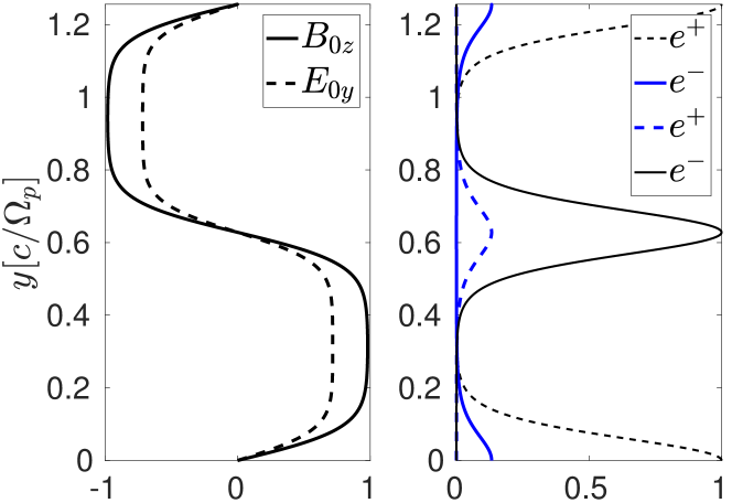
Figure 1: Stationary solution to the fluid-Maxwell equations in an $e^{-}e^{+}$ system composed of a hot beam ($T_{b0}=1$, $\beta_{b0}=-0.995$) and a background cold plasma ($N_{p}/N_{b}=1$, $T_{p0}=0.1$, $\beta_{p0}=0.995$). The vector potential maximum is $a_{0}=0.25$, resulting in a wavelength $\lambda_{0}=1.26\,c/\Omega_{p}$. Left panel: $B_{0z}(y)$ (solid line) and $E_{0y}(y)$ (dashed line), normalized to $mc\Omega_{p}/e$, where $\Omega_{p}$ is the relativistic frequency associated with the peak electron (or positron) frequency. Right panel: Density profiles of the electrons (solid lines) and positrons (dashed lines) in the hot (blue) and cold (black) beams, normalized to the maximum cold-beam electron (or positron) density.

Analytic expressions for the wavelength $\lambda_{0}$ can be derived for two symmetric pair beams ($|\beta_{b0}|=|\beta_{p0}|=\beta_{0}$, $\gamma_{b0}=\gamma_{p0}=\gamma_{0}$, $T_{b0}=T_{p0}=T_{0}$, $N_{b}=N_{p}=N$), which can then serve as initial guesses for the boundary value solver. Due to the symmetry, the electrostatic field vanishes. Setting $\phi_{0}=0$, the problem reduces to solving Eq. (13). Let us first consider the weak-field limit, in which case we readily obtain

$$\lambda_{0}=\frac{\pi\sqrt{T_{0}}}{\beta_{0}\gamma_{0}}\ \frac{c}{\omega_{p}}\,,$$ (16)

where $\omega_{p}=\sqrt{4\pi e^{2}N/m}$ is the relativistic plasma frequency of a single (electron or positron) species, expressed in terms of the density parameter $N$ appearing in Eq. (12).

In the more general, nonlinear symmetric case, the periodicity $\lambda_{0}$ depends on $a_{0}$ through the following exact analytic expression

$$\lambda_{0}=\frac{2\sqrt{T_{0}}}{\beta_{0}\gamma_{0}}K\left[-\sinh^{2}\left(\frac{\xi}{2}\right)\right]\frac{c}{\omega_{p}}\,,$$ (17)

with the nonlinearity parameter

$$\xi=\frac{\gamma_{0}\beta_{0}a_{0}}{T_{0}}\,,$$ (18)

and $K(k)$, the complete elliptic integral of the first kind. Moreover, the magnetic field and density profiles can be expressed as

$$B_{0z}(y) =\frac{2uT_{0}}{\gamma_{0}\beta_{0}}\frac{\textrm{dn}\left[u\left(y-\lambda_{0}/4\right),\kappa^{2}\right]}{\textrm{cn}\left[u\left(y-\lambda_{0}/4\right),\kappa^{2}\right]}\frac{mc^{2}}{e}\,,$$ (19)

$$n_{\alpha 0}(y) =N\left\{\frac{\textrm{cn}\left[u\left(y-\lambda_{0}/4\right),\kappa^{2}\right]}{1\pm\textrm{sn}\left[u\left(y-\lambda_{0}/4\right),\kappa^{2}\right]}\right\}^{2}\,,$$ (20)

where $\textrm{sn}(u,k)$, $\textrm{cn}(u,k)$ and $\textrm{dn}(u,k)$ are the Jacobi elliptic functions. The $\pm$ sign in Eq. (20) denotes the sign of the current of species $\alpha$. The parameters $u$ and $\kappa$ are defined as

$$u =2\frac{\gamma_{0}\beta_{0}}{\sqrt{T_{0}}}\sinh\left(\xi/2\right)\frac{\omega_{p}}{c}\,,$$ (21)

$$\kappa =\coth\left(\xi/2\right)\,.$$ (22)

A given species is in a strongly nonlinear (pinched) regime if $\xi_{\alpha}\equiv\gamma_{\alpha}\beta_{\alpha}a_{0}/T_{\alpha}\gg 1$ (i.e., $\kappa\to 1^{+}$), in which case its peak density greatly exceeds $N_{\alpha}$. If this condition is fulfilled by all species, the system then consists of a periodic chain of well-separated neutral current sheets, which tend to the Harris solution Harris_1962 ; Zelenyi_1979 ; Balikhin_2008 , widely used in magnetic reconnection studies. This result readily follows from taking the $\kappa\to 1^{+}$ limit of the Jacobian elliptic functions Byrd_1954 involved in Eqs. (19) and (20) around the density maximum. Applying the latter limit to (20) leads to

$$n_{0}(y) \simeq\frac{N}{4}\exp(u\lambda_{0}/2)\cosh^{-2}(uy)$$ (23)

$$\simeq Ne^{\xi}\cosh^{-2}(uy)\,,$$ (24)

which corresponds to a Harris-type relativistic current sheet Zelenyi_1979 ; Balikhin_2008 with maximum density

$$\max_{y}n_{0}=Ne^{\xi}\,,$$ (25)

and characteristic width

$$l =u^{-1}$$ (26)

$$\simeq\frac{\sqrt{T_{0}}e^{-\xi/2}}{\gamma_{0}\beta_{0}}\frac{c}{\omega_{p}}=\frac{\sqrt{T_{0}}}{\gamma_{0}\beta_{0}}\frac{c}{\Omega_{p}}\,.$$ (27)

In the same limit, Eq. (19) becomes (for $l\ll y\ll\lambda_{0}$)

$$\frac{B_{0z}^{2}(y)}{8\pi} \simeq 2T_{0}mc^{2}Ne^{\xi}$$ (28)

$$\simeq 2T_{0}mc^{2}\max_{y}n_{0}\,,$$ (29)

which expresses the expected balance between magnetic and thermal pressures in a current filament.

II.3 Perturbative system

We now linearize the fluid-Maxwell equations (1)-(5) around the initial state described by Eqs. (6)-(8). Since the steady state is invariant along $x$, the first-order quantities are taken in the form $\delta b(y)e^{ik_{x}x-i\omega t}$, where $k_{x}$ is the longitudinal wavenumber, $\omega=\omega_{r}+i\Gamma$ is the complex frequency and $\delta b(y)$ is the eigenfunction. The fluid equations are closed assuming an adiabatic equation of state

$$p_{\alpha}\propto n_{\alpha}^{\Gamma_{\mathrm{ad,\alpha}}}\,.$$ (30)

In the following, we will take $\Gamma_{\mathrm{ad,\alpha}}=4/3$ in a relativistically hot beam ($T_{\alpha}\gtrsim 1$) and $\Gamma_{\mathrm{ad,\alpha}}=5/3$ otherwise.

The linearized system, detailed in Appendix A, consists of 10 independent coupled homogenous differential equations with $y$-periodic coefficients that depend on the equilibrium quantities. This system can be written in the compact form

$$\partial_{y}\bm{x}(y)=\bm{\Xi}(y,\omega,k_{x})\bm{x}(y)\,,$$ (31)

where $\bm{x}(y)=(\delta e_{x},\delta b_{z},\delta p_{1},...\delta p_{4},\delta v_{y1},...,\delta v_{y4})$ is a 10-component vector containing the first-order variables, and $\bm{\Xi}(y,\omega,k_{x})$ is a $10\times 10$ $y$-periodic matrix. This equation can be solved using the Floquet theory Grimshaw_1993 as explained in the next section.

III Floquet analysis

III.1 General method

We now recall the basics of the Floquet theory Grimshaw_1993 used to solve Eq. (31). For the sake of clarity, the vectors and matrices are written in lowercase and uppercase, respectively. Equation (31) has the general form

$$\partial_{y}\bm{x}(y)=\bm{\Xi}(y)\bm{x}(y)\,,$$ (32)

where $\bm{x}$ is a $n$-dimensional vector and $\bm{\Xi}(y)$ is a $n\times n$ periodic matrix, i.e.,

$$\bm{\Xi}(y)=\bm{\Xi}(y+\lambda),\ \forall y\in\mathbb{R}.$$ (33)

Here, $\lambda$ is the minimal periodicity of the system satisfying the relation (33). We now introduce the fundamental matrix

$$\bm{M}(y)=\Big{[}\left[\bm{x}_{1}(y)\right]...\left[\bm{x}_{n}(y)\right]\Big{]}\,,$$ (34)

where $\bm{x}_{j}(y),...,\bm{x}_{n}(y)$ are $n$ linearly independent solutions to Eq. (32). $\bm{M}(y)$ satisfies the differential equation

$$\partial_{y}\bm{M}(y)=\bm{\Xi}(y)\bm{M}(y)\,.$$ (35)

According to the Floquet theory, $\bm{M}$ has the form

$$\bm{M}(y)=\bm{P}(y)\bm{\Sigma}(y)\,,$$ (36)

where

$$\bm{\Sigma}(y)=\textrm{diag}\Big{[}e^{\mu_{1}y},...,e^{\mu_{n}y}\Big{]}\,,$$ (37)

with $\mu_{j},...,\mu_{n}$ the so-called characteristic Floquet exponents. The matrix $\bm{P}(y)$ is composed of $n$ vector-valued periodic functions:

$$\bm{P}(y)=\Big{[}\left[\bm{p}_{1}(y)\right]...\left[\bm{p}_{n}(y)\right]\Big{]}$$ (38)

such that

$$\bm{p}_{j}(y)=\bm{p}_{j}(y+\lambda),\ \forall y\in\mathbb{R}.$$ (39)

The real parts of the Floquet exponents are well defined, yet their imaginary parts are not unique since a phase shift of $2\pi/\lambda_{0}$ can be applied indifferently to the Floquet exponents or $\bm{P}(y)$.

The diagonal elements of $\bm{\Sigma}(\lambda)=\textrm{diag}[\sigma_{1},...,\sigma_{n}]$ are called the characteristic multipliers, which can be obtained as the eigenvalues of the non-singular constant matrix $\bm{B}$ defined by

$$\bm{B}=\bm{M}^{-1}(y)\bm{M}(y+\lambda)\,.$$ (40)

Introducing $\bm{b}_{1},...,\bm{b}_{n}$ the eigenvectors of $\bm{B}$, and defining the matrix

$$\bm{S}=\Big{[}\left[\bm{b}_{1}\right]...\left[\bm{b}_{n}\right]\Big{]}\,,$$ (41)

we have

$$\bm{\Sigma}(\lambda)=\bm{S}^{-1}\bm{B}\bm{S}\,,$$ (42)

so that

$$\bm{P}(y)=\bm{\Sigma}(y)\ \bm{S}\ \bm{\Sigma}^{-1}(y)\,.$$ (43)

An important result is that the eigenvectors and eigenvalues of $\bm{B}$ do not depend on the choice of initial conditions. For a given set of $\bm{x}_{j}(y),...,\bm{x}_{n}(y)$, numerically computed over a period, we evaluate $\bm{B}=\bm{M}^{-1}(0)\bm{M}(\lambda)$ and solve for its eigenvalues and eigenmodes. In practice, for a given value of $k_{x}\in\mathbb{R}$, we scan a region of the complex $\omega$-space, and retain only the temporally unstable eigenmodes, i.e., those with purely real transverse wavenumbers, $k_{y}\equiv-i\mu_{i}\in\mathbb{R}$. Inverting the results readily gives the dispersion relation $\omega(k_{x},k_{y})$. This technique, previously used in Ref. Romeiras_1986 , has the advantage of not requiring the infinite Hill’s determinant to be derived, as is commonly done when applying the Floquet theory to systems periodic in space time (see, e.g., Quesnel_1997 ).

In order to gauge the accuracy of our results, we check that the exact relation

$$\textrm{det}\ \bm{B}=\textrm{exp}\left\{\int_{0}^{\lambda}\operatorname{Tr}\left[\bm{\Xi}(y)\right]dy\right\}\,.$$ (44)

is well satisfied. Also, due to the possible presence of spatially fast-growing modes ($\Im k_{y}\neq 0$), we use initial conditions such that $\bm{x}_{j}^{i}(\lambda/2)=\delta_{j}^{i}$ ($i,j=1,...,n$).

III.2 Instability of two homogeneous symmetric counterstreaming pair beams

We first address the problem of a homogeneous plasma system (or, equivalently, vanishing fields), in which case we expect to recover the standard linear dispersion relation Bret_2010a . Specifically, we consider two symmetric counterstreaming pair beams with $T_{0}=1$ and $\gamma_{0}=10$. Owing to the symmetry of the system, the complex frequency is purely imaginary ($\omega=i\Gamma$), and hence the search for the $\omega$ values yielding $k_{y}\in\mathbb{R}$ is restricted to a 1D parameter space (at fixed $k_{x}$). The results of the Floquet solver are compared with those obtained from the homogeneous linear dispersion relation. This dispersion relation, derived from linearizing Eqs. (1)-(5) in the homogeneous limit, takes on the form of a 10th-order polynomial. This relation is too lengthy to be written here, but a more compact expression of it can be obtained using the covariant formalism developed in Ref. Achterberg_2007_I . For each point in the $(k_{x},k_{y})$ Fourier space, we compute the roots $\omega(k_{x},k_{y})$ of this polynomial and retain the solution with maximum (and positive) $\Im\omega$. For the Floquet solver, we sample the parameter space $(\Gamma,k_{x})\in\mathbb{R}^{+}\times\mathbb{R}^{+}$, and look for eigenmodes with $k_{y}\in\mathbb{R}$.

Figure 2 confirms that the two methods give identical growth-rate maps. In the Floquet case (bottom panel), the cruder resolution in $k_{y}$ follows from the chosen resolution in $\Gamma$. As expected Bret_2010a , the system gives rise to a broad unstable spectrum, characterized by dominant, purely tranverse CFI modes (with $k_{x}=0$) and a continuum of sub-dominant oblique modes extending up to infinite $k$. A more physical kinetic description would evidently lead to a bounded unstable spectrum due to Landau damping of high-$k$ modes Bret_2010a .

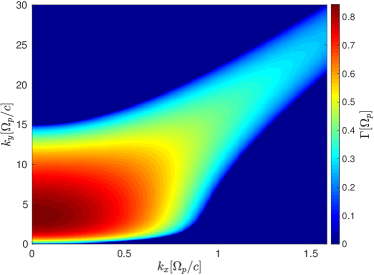
Figure 2: Instability growth rates ($\Gamma$) in the $(k_{x},k_{y})$ plane for two symmetric counterstreaming pair beams with $T_{0}=1$ and $\gamma_{0}=10$, as obtained from the linear dispersion relation (top) and the Floquet method (bottom).

IV 1D instability of weakly nonlinear symmetric filaments

The purely transverse CFI is the dominant instability arising in a symmetric relativistic two-beam plasma in the homogeneous limit Bret_2010a . As will be shown in V, the dominant unstable mode in a periodic system of weakly pinched filaments remains purely transverse ($k_{x}=0$), and can be viewed as a filament merging instability (FMI). In this section, we examine the properties of this instability in a purely 1D geometry.

IV.1 Floquet analysis

We study the stability of a stationary symmetric two-beam system characterized by $T_{0}=1$, $\gamma_{0}=10$ and $a_{0}=0.04$ ($\xi=0.4$), associated with a fundamental wavelength $\lambda_{0}\simeq 0.38\,c/\Omega_{p}$. We solve the perturbative eigenvalue problem using the method previously explained with $k_{x}=0$ and $\omega=i\Gamma$ purely imaginary. For each sampled value of $\Gamma$, we find two solutions with real positive $k_{y}$, and their symmetric negative counterparts (corresponding to the same physical modes). Figure 3 plots the growth rate $\Gamma$ as a function of the characteristic Floquet exponent $k_{y}\in[0,2\pi/\lambda_{0}]$. Since $\Gamma(k_{y})$ is even, it should remain unchanged under the operation $k_{y}\rightarrow k_{y}+2n\pi/\lambda_{0}$ ($n\in\mathbb{N}$). For clarity, we have chosen to unfold $\Gamma(k_{y})$ over the range $[0,2\pi/\lambda_{0}]$, but one could have alternatively chosen the range $[0,\pi/\lambda_{0}]$, yielding a double-valued curve. Unstable modes are found up to $k_{y}\simeq 12.2\,\Omega_{p}/c$, to be compared with the fundamental wavenumber $k_{0}\equiv 2\pi/\lambda_{0}\simeq 16.5\,\Omega_{p}/c$. The maximum growth rate, $\Gamma_{\mathrm{max}}=0.69\,\Omega_{p}$, occurs at $k_{y,\mathrm{max}}\simeq 2.85\,\Omega_{p}/c$. We also plot the CFI growth rates associated with the same values of $T_{0}$ and $\gamma_{0}$. The two curves present similar shapes, but the plasma inhomogeneity tends to reduce both the maximum growth rate and wavenumber range of the instability.

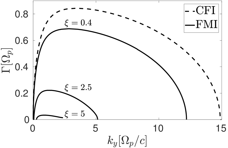
Figure 3: Growth rate ($\Gamma$, solid curve) of the FMI as a function of the characteristic Floquet exponent ($k_{y}$). The unperturbed periodic system consists of two symmetric counterstreaming pair beams with $T_{0}=1$, $\gamma_{0}=10$. Three different field strengths, $a_{0}=0.04,0.25,0.5$ (i.e., $\xi=0.4,2.5,5$), are considered, which are associated with fundamental wavenumbers $k_{0}=16.5,8.03,4.88\,\Omega_{p}/c$ (i.e., $\lambda_{0}=0.38,0.78,1.28\,c/\Omega_{p}$). For comparison, the dashed curve plots the growth rate of the CFI in the homogeneous limit with the same ($T_{0},\gamma_{0}$) parameters.

The spatial profiles of the components $(\delta E_{x},\delta E_{y},\delta B_{z},\delta v_{1y},\delta d_{1})$ of the fastest-growing FMI eigenmode are displayed in Fig. 4. Due to the symmetric configuration, only the perturbation of the positron fluid with positive velocity are shown. Both the real and imaginary parts of the eigenfunctions are plotted, showing that they only differ by a constant phase of $\sim\pi/2$. The electromagnetic field perturbations $(\delta E_{x},\delta B_{z})$ are well described by a single harmonic function with wavenumber $k_{y,\mathrm{max}}$, so that $|\delta E_{x}/\delta B_{z}|\simeq\Gamma_{\mathrm{max}}/k_{y,\rm max}\simeq 0.26$. By contrast, $\delta v_{1y}$, $\delta d_{1}$ show a richer harmonic content, with modulations at the scale of $\lambda_{0}$. Yet the charge density modulations cancel out to yield a zero electrostatic field $\delta E_{y}$.

The space-time evolution of the dominant FMI mode is depicted in Fig. 5 by plotting the total apparent density of species 1, $d_{1}(y,t)=d_{10}(y)+\epsilon\delta d_{1}(y)e^{\Gamma t}$ (where $\epsilon\ll 1$). For the sake of being illustrative, $d_{1}(y,t)$ is evolved up to the point where it vanishes, i.e, strictly speaking beyond the linear regime. One clearly sees that the instability has the effect of creating bunches of three or four filaments, whose density rises as they coalesce. The filaments surrounding the merging ones also experience magnetic attraction, albeit weaker. In the nonlinear saturated stage, the system will then be reorganized into a quasiperiodic filamentary pattern with a characteristic wavelength about 6 times longer than in its unperturbed state.

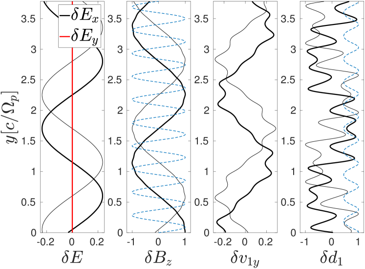
Figure 4: Spatial structure of the dominant FMI eigenmode for the parameters of Fig. 3. The thick (resp. thin) solid lines plot the real (resp. imaginary) parts of the eigenfunctions. The perturbed quantities are, from left to right, the inductive electric field ($\delta E_{x}$, black), the electrostatic electric field ($\delta E_{y}$, red), the magnetic field ($\delta B_{z}$), the transverse velocity ($\delta v_{1y}$), and the lab-frame density of plasma species 1 ($\delta d_{1}$). $\delta E_{x}$, $\delta E_{y}$ and $\delta B_{z}$ are normalized to $\max_{y}|\delta B_{z}|$, while $\delta v_{1y}$ and $\delta d_{1}$ are normalized to $\max_{y}|\delta d_{1}|$. The blue dashed lines plot the corresponding unperturbed quantities normalized to their maximum value.

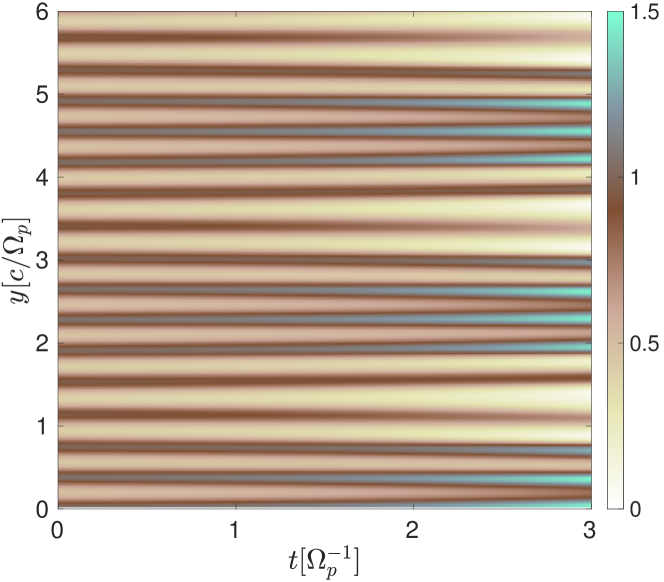
Figure 5: Space-time evolution of the density component, $d_{1}=d_{10}(y)+\delta d_{1}(y)e^{\Gamma t}$ (normalized to $\mathrm{max}_{y}d_{10}$), of the fastest-growing FMI eigenmode. The parameters are those of Fig. 3. The evolution is stopped slightly before $d_{1}$ becomes negative.

IV.2 1D PIC simulation

To support the results of the Floquet analysis, we have performed a 1D3V PIC simulation (1D in space and 3D in momentum) using the code calder Lefebvre_2003 . In accordance with the theoretical calculation, the plasma comprises two counterstreaming pair beams, made up of a total of four species. Each species $\alpha$ is initialized with a drifting Jüttner-Synge momentum distribution:

$$f_{\alpha 0}(y,\bm{p}) =N_{\alpha}\exp\left\{-\frac{\gamma_{\alpha 0}}{T_{\alpha 0}}\left[\gamma(\bm{p})+\frac{q_{\alpha}\phi_{0}(y)}{mc^{2}}\right.\right.$$

$$\left.\left.-\frac{\beta_{\alpha}}{mc}\left(p_{x}+\frac{q_{\alpha}}{c}\beta_{\alpha 0}A_{0x}(y)\right)\right]\right\}\,,$$ (45)

where the equilibrium potentials $(\phi_{0},A_{0x})$ are numerical solutions to Eqs. (13) and (14). In the present symmetric case, we have $\phi_{0}(y)=0$, and hence the initial electromagnetic fields are $B_{0z}(y)=-\partial_{y}A_{0x}$ and $E_{0x}(y)=E_{0y}(y)=0$. The physical parameters are those considered in the previous section: $T_{0}=1$, $\gamma_{0}=10$ and $a_{0}=0.04$, giving $\lambda_{0}=0.38c/\Omega_{p}$. The simulation domain is $50\,\lambda_{0}$ long, allowing the unstable modes to be accurately resolved. The mesh size is $\Delta y=\lambda_{0}/100=0.0038c/\Omega_{p}$ and the time step is $\Delta t=0.99\,\Delta x/c$. Each cell initially contains 1000 macroparticles per species. Periodic boundary conditions are used for both fields and particles. The instability is seeded by thermal noise alone.

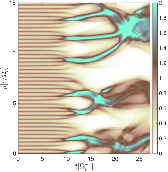
Figure 6: 1D PIC simulation with the parameters $T_{0}=1$, $\gamma_{0}=10$ and $a_{0}=0.04$ (as in Fig. 3): space-time evolution of the density of plasma species 1 (normalized to its initial peak value).

Figure 6 displays the space-time evolution of the density of species 1 (positrons moving along $x>0$). A first instability stage is observed to last until $t\lesssim 10\,\Omega_{p}^{-1}$: it is characterized by mergers between clusters of 3-4 neighboring filaments, consistent with the theoretical prediction of Fig. 5. The larger and denser filaments resulting from this primary instability undergo successive merging stages, leading to increasingly wide and spaced filaments.

The linear properties of the early-time FMI can be further quantified from the time evolution of the total electromagnetic energies (Fig. 7) and of the Fourier transformed magnetic field $|B_{z}(k_{y},t)|^{2}$ (Fig. 8). In Fig. 7, the instability is seen to emerge from the electric thermal noise at $t\simeq 2\,\Omega_{p}^{-1}$, at which time the inductive electric field ($E_{x}$) energy starts to rise exponentially. Since the magnetic field energy is initialized at a finite level (contrary to the initially vanishing electric field), the effect of the instability on it is only discernible after $t\simeq 7\,\Omega_{p}^{-1}$. Both $E_{x}$ and $B_{z}$ energies then grow as $\propto e^{2\Gamma_{\mathrm{PIC}}t}$ where $\Gamma_{\mathrm{PIC}}\simeq 0.80\,\Omega_{p}$ is the best-fitting growth rate over $4\leq t\leq 8\,\Omega_{p}^{-1}$. This value is comparable with the theoretical prediction $\Gamma_{\mathrm{max}}\simeq 0.69\,\Omega_{p}$, the small difference being ascribed to kinetic effects. In particular, one may question the accuracy of the adiabatic closure relation: our choice of $\Gamma_{\mathrm{ad}}=4/3$ is somewhat dubious as the temperature $T_{0}=1$ is not highly relativistic, and, more importantly, as it implies three degrees of freedom (whereas our PIC simulation is only 1D). We have checked that using $\Gamma_{\mathrm{ad}}=2$, the value expected in a relativistically hot 1D plasma, gives a growth rate $\Gamma_{\mathrm{max}}\simeq 0.80\,\Omega_{p}$ (for $k_{y,\rm max}\simeq 2.3\,\Omega_{p}/c$), closer to the simulation results. The eigenfunctions of the dominant mode are hardly modified by the choice of $\Gamma_{\rm ad,\alpha}$. They predict an order of magnitude difference in the $B_{z}$ and $E_{x}$ energies, which is well reproduced in the simulation during the period $7\lesssim t\lesssim 10\,\Omega_{p}^{-1}$ (Fig. 7). Also, the non-increasing $E_{y}$ energy is consistent with the theoretical prediction.

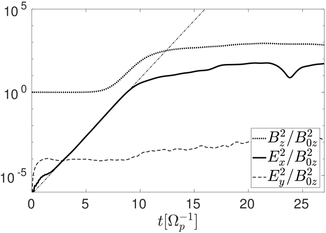
Figure 7: Time evolution of the electromagnetic energies (spatially integrated and normalized to the initial magnetic energy). The initial simulation parameters are those of Fig. 6. The magnetic ($B_{z}$) energy is plotted as a dotted line, the inductive ($E_{x}$) energy as a thick solid line and the electrostatic ($E_{y}$) energy as a dashed line. The thin dotted-dashed line represents the best-fitting exponential curve over $5\leq t\leq 10\,\Omega_{p}^{-1}$, with a growth rate $\Gamma_{\mathrm{PIC}}\simeq 0.8\,\Omega_{p}$.

Figure 8 shows that the FMI mainly develops in the wavenumber range $1\lesssim k_{y}\lesssim 6\,\Omega_{p}/c$, as expected from theory (Fig. 3). Note that, in principle, the wavenumbers $k_{y}$ in this Fourier spectrum should not be directly compared to the characteristic Floquet exponents (see Fig. 3) since the eigenfunctions are of the form $\delta b(y)=\sum_{n\in\mathbb{N}}\delta b_{n}e^{i(k_{y}+nk_{0})y}$, with $k_{0}$ being the fundamental wavenumber of the stationary state and $\delta b_{0}$ being not necessarily dominant. Yet for the weakly nonlinear filaments considered, the magnetic-field eigenfunction is well approximated by a single harmonic term $\delta B_{z}\sim\delta b_{0}e^{ik_{y}y}$ (see Fig. 4), so that the Fourier wavenumbers can be assimilated to good accuracy to the Floquet exponents. The growing modes appear to saturate at $t\simeq 10\,\Omega_{p}^{-1}$, causing depletion of the fundamental magnetic mode (located at $k_{0}=16.5\,\Omega_{p}/c$). From this time onwards, the magnetic energy in the system is essentially contained in the unstable spectral range ($k_{y}\lesssim 6\,\Omega_{p}/c$), leading to an exponential growth of the total magnetic energy (Fig. 8). As time increases, the magnetic spectrum progressively shrinks to low $k_{y}$ due to successive filament mergers, which account for the modulations of the $E_{x}$ energy in the saturated stage (Fig. 7).

A rough estimate of the gain in magnetic field energy at saturation can be derived from Ampère’s equation expressed at the initial and saturation times: $B_{0}\propto 2\exp(-\xi)\sinh(\xi)d_{0}\lambda_{0}$ and $B_{\rm sat}\propto d_{\rm sat}\lambda_{\rm sat}$, with $d_{\rm sat}$ and $\lambda_{\rm sat}$ being, respectively, the apparent density of a given species and the typical wavelength at saturation. The factor $2\exp(-\xi)\sinh(\xi)$ accounts for the significant overlap of the weakly inhomogeneous, counterstreaming flows in the initial state (such overlap is neglected at saturation) and the mean flow velocity is assumed to remain close to $c$. Making use of mass conservation, $d_{\rm sat}\lambda_{\rm sat}=d_{0}\lambda_{0}(k_{0}/k_{\rm max})$, one then predicts $(B_{\rm sat}/B_{0})^{2}\simeq\left(\exp(\xi)/2\sinh(\xi)\right)^{2}(k_{0}/k_{\rm max})^{2}$. Given $\xi=0.4$ and the theoretical prediction $k_{0}/k_{\rm max}\simeq 16.5/2.85$, one obtains $(B_{\rm sat}/B_{0})^{2}\simeq 120$, in fair agreement with the simulated value measured at $t\simeq 10\,\Omega_{p}^{-1}$ [Fig. (7)].

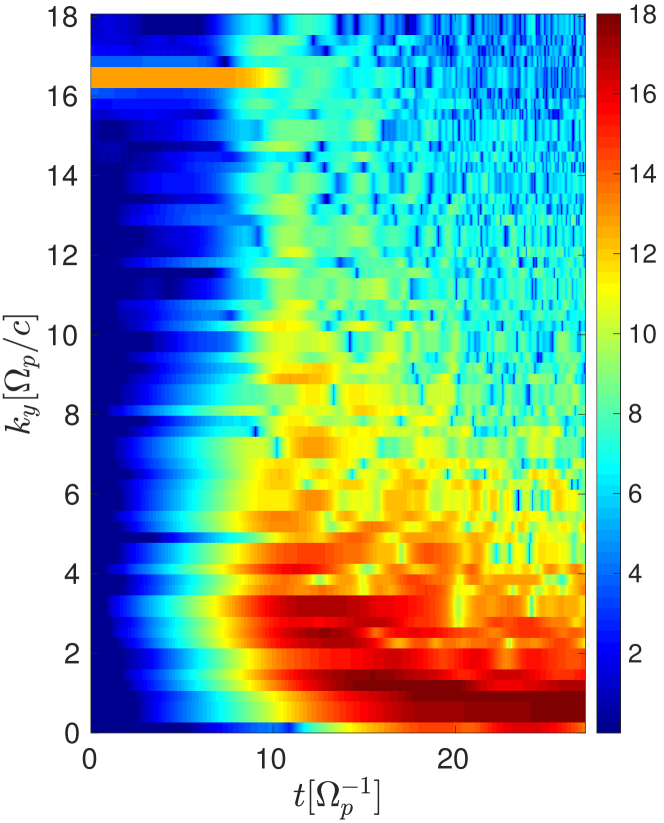
Figure 8: Time evolution of the Fourier transformed magnetic field, $|B_{z}(k_{y},t)|^{2}$ (in $\log_{10}$ scale). The initial simulation parameters are those of Fig. 6. The bright spectral line at $k_{y}\simeq 16.5\,\Omega_{p}/c$ corresponds to the fundamental wavenumber of the equilibrium state.

V 2D instability of strongly nonlinear symmetric filaments

In this section, we push the stationary system far into the nonlinear regime, so that the equilibrium filaments get strongly pinched and the magnetic field can no longer be approximated by a single harmonic. We will demonstrate that the increasing nonlinearity of the system causes its dominant eigenmode to evolve from a purely tranverse FMI to a drift kink-type instability (DKI). To show this, we consider the same symmetric two-beam system as before (with $T_{0}=1$ and $\gamma_{0}=10$), but increase the vector potential amplitude from $a_{0}=0.04$ to $a_{0}=0.5$ (i.e., the nonlinearity parameter rises from $\xi=0.4$ to $\xi=5$).

V.1 Floquet analysis

Figure 3 shows that for $\xi=2.5$ the FMI growth rate exhibits a significantly reduced maximum value ($\Gamma_{\rm max}\simeq 0.22\,\Omega_{p}$ at $k_{y,\rm max}\simeq 1.29\,\Omega_{p}/c$) and upper cutoff ‘wavenumber’ $k_{y}\simeq 5.1\,\Omega_{p}/c$. Also, it presents a nonzero lower cutoff $k_{y}\simeq 0.06\,\Omega_{p}/c$ (hardly visible in Fig. (3)). When the nonlinearity is further strengthened ($\xi=5$), the lower cutoff increases to $k_{y}\simeq 0.27\,\Omega_{p}/c$ and the $\Gamma$ curve abruptly stops at $k_{y}=k_{0}/2=2.45\,\Omega_{p}/c$ (where $k_{0}\simeq 4.88\,\Omega_{p}$ is the corresponding fundamental wavenumber). The latter discontinuity is a typical feature of unstable waves in periodic media (e.g., see Romeiras_1978 ; Romeiras_1986 ). Actually, this gap becomes discernible for $\xi\gtrsim 3.5$, and results in a progressive quelling of the modes in the range $k_{0}/2\leq k_{y}\leq k_{0}$. Stabilization of the low-$k_{y}$ modes is also specific to the strongly inhomogeneous regime; this mechanism underlines a recently proposed scheme, which exploits density ripples to mitigate the CFI in the laser-plasma context Mishra_2014 .

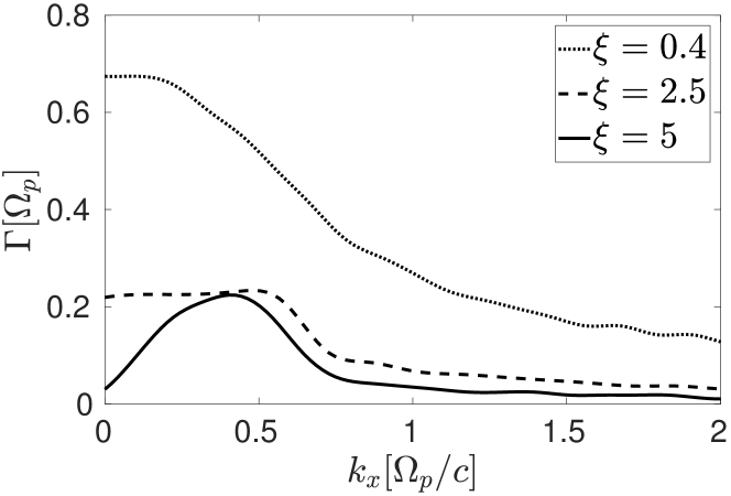
Figure 9: Growth rate $\Gamma$, maximized over $k_{y}$, as a function of the longitudinal wavenumber $k_{x}$ and the nonlinearity level $\xi$. The symmetric two-beam system is characterized by $T_{0}=1$ and $\gamma_{0}=10$.

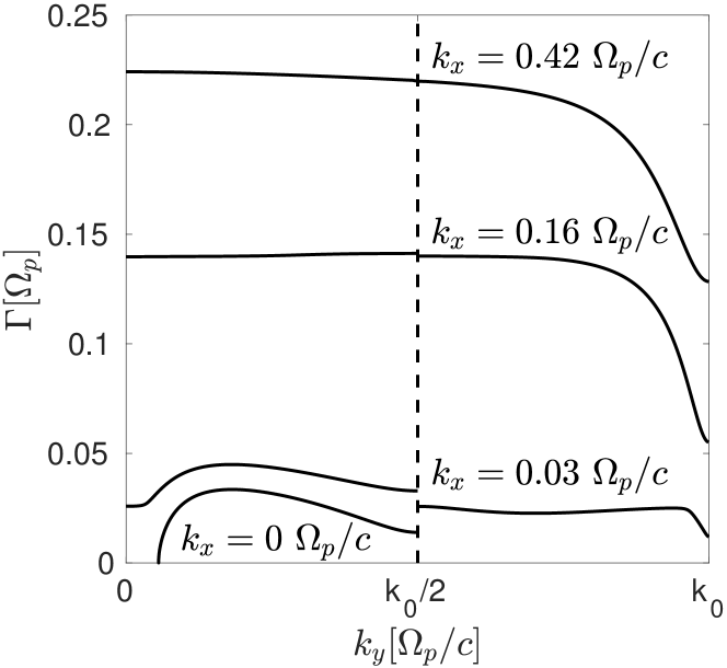
Figure 10: Instability growth rate ($\Gamma$) as a function of the characteristic Floquet exponent ($k_{y}$) for different values of $k_{x}$. The stationary symmetric system is characterized by $T_{0}=1$, $\gamma_{0}=10$ and $\xi=5$, yielding $\lambda_{0}=1.28\,c/\Omega_{p}$.

We now perform a full 2D stability analysis of the equilibrium filamentary state by considering nonzero values of the longitudinal wavenumber $k_{x}$. Since the two-beam system remains symmetric, the $\omega$ sampling space is still restricted to the imaginary axis. In Fig. 9, we plot the $k_{y}$-maximized growth rate as a function of $k_{x}$ for various degrees of nonlinearity. As previously discussed, the dominant mode at $\xi=0.4$ is the purely tranverse ($k_{x}=0$) FMI. As we increase $\xi$, the growth rates globally decrease, yet the FMI modes near $k_{x}=0$ are the most severely weakened. At $\xi=2.5$, the growth rate curve exhibits a plateau at $\Gamma\simeq 0.22\,\Omega_{p}$ in the interval $0\leq k_{x}\leq 0.6\,\Omega_{p}/c$. On further raising $\xi$, the low-$k_{x}$ FMI modes are increasingly stabilized, while modes around $k_{x}\gtrsim 0.4\,\Omega_{p}/c$ are only weakly diminished. At $\xi=5$, this trend leads to the growth rate curve peaking at $k_{x,\rm max}\simeq 0.42\,\Omega_{p}$.

Figure 10 shows the $k_{y}$-dependence of $\Gamma$ for $\xi=5$ and different values of $k_{x}$. The $k_{x}=0$ curve is identical to that plotted in Fig. 3, as discussed above. At $k_{x}=0.03\,\Omega_{p}/c$, the entire range $0\leq k_{y}\leq k_{0}$ is destabilized, with finite and increased growth rates everywhere (even at $k_{y}=0$ and $k_{0}$). A gap is still present at $k=k_{0}/2$ and the dominant mode remains located at a relatively low $k_{y}\simeq 0.8\,\Omega_{p}/c$. Further increasing $k_{x}$ strengthens all modes, but especially those with $k_{y}>k_{0}/2$, so that the gap at $k_{y}=k_{0}/2$ is progressively bridged. The $\Gamma$ curves then tend to form a quasi-plateau in the $0\leq k_{y}<k_{0}/2$ range, and drop to a finite value for $k_{y}\,\to\,k_{0}$.

For $k_{x}=0.42\,\Omega_{p}/c$, the growth rates are bounded between $\Gamma=0.22\,\Omega_{p}$ ($k_{y}\to 0$) and $\Gamma=0.13\,\Omega_{p}$ ($k_{y}\to k_{0}$), while the discontinuity at $k_{y}=k_{0}/2$ is no longer visible. The eigenmodes associated with $k_{y}=0$ and $k_{y}=k_{0}$ have a minimal periodicity that is equal to, or is a divisor of the fundamental period of the equilibrium system. Their transverse spatial structure is displayed in Figs. 11 and 12, respectively. We expect the intermediate eigenfunctions (with $0<k_{y}<k_{0}$) to evolve smoothly between these two limits. Each figure plots the $(\delta E_{x},\delta E_{y},\delta B_{z})$ and $(\delta v_{1y},\delta v_{1x},d_{1})$ components of the eigenmode, respectively normalized to $\mathrm{max}_{y}|B_{z}|$ and $\mathrm{max}_{y}|d_{1}|$. The thick and thin solid lines represent, respectively, the real and imaginary parts of each quantity. The perturbed magnetic (resp. density) profile of both eigenmodes is even (resp. odd) with respect to the filament center, which is indicative of DKI Zenitani_2007 . The two modes mainly differ in the oscillation phase between opposite-current filaments. For the dominant mode, the magnetic perturbations at the center of two neighboring current filaments (e.g., at $y=0$ and $y=0.64\,c/\Omega_{p}$) are of opposite sign, so that all filaments oscillate in phase. For the sub-dominant mode, adjacent filaments of opposite current see magnetic perturbations of the same sign, and hence they oscillate out of phase. As a consequence, the electromagnetic profiles of the two modes have different periodicities: the dominant mode has the same minimal periodicity ($\lambda_{0}$) as the equilibrium system, whereas the sub-dominant mode has a minimal periodicity of $\lambda_{0}/2$.

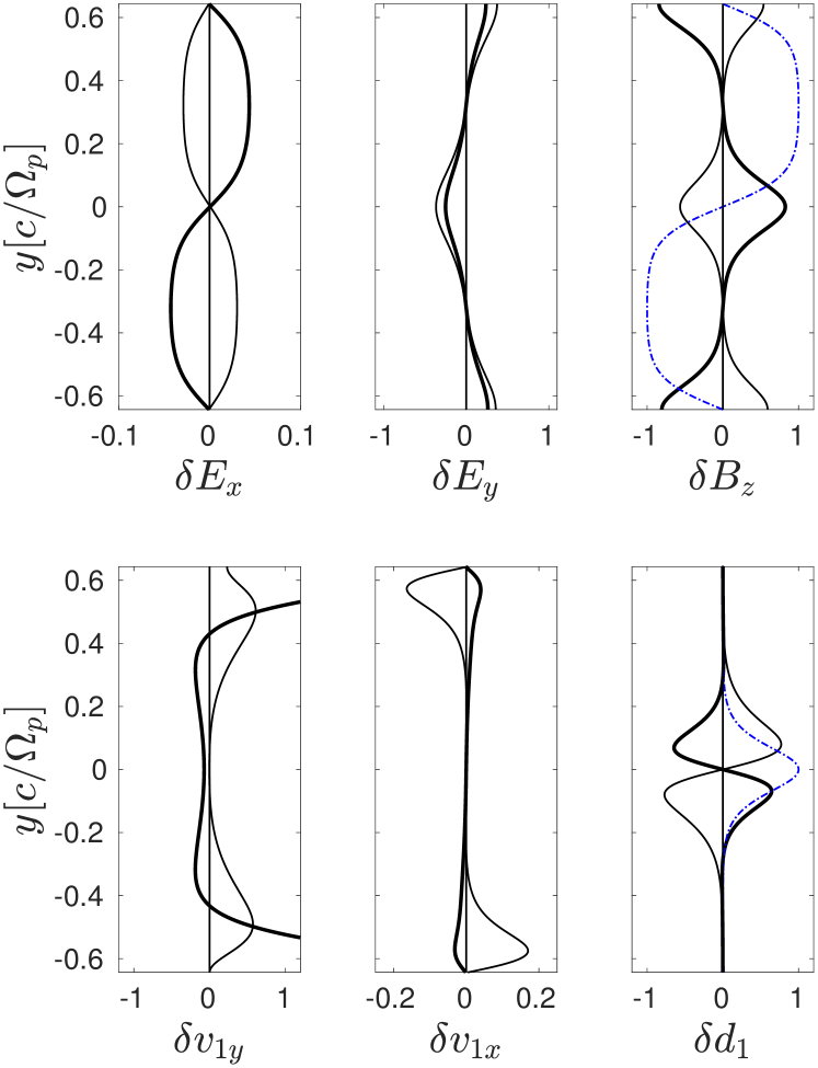
Figure 11: Transverse spatial structure of the eigenmode characterized by $\Gamma=0.22\,\Omega_{p}$, $k_{y}=0$ and $k_{x}=0.42\,\Omega_{p}/c$ (same parameters as in Fig. 9). This eigenmode is the dominant one in Figs. 9 and 10. The thick (resp. thin) solid lines plot the real (resp. imaginary) part of the eigenfunctions. The perturbed quantities are, from left to right and top to bottom, $\delta E_{x}$, $\delta E_{y}$, $\delta B_{z}$, normalized to $\mathrm{max}_{y}|\delta B_{z}|$ and $\delta v_{1x}$, $\delta v_{1y}$ and $\delta d_{1}$, normalized to $\mathrm{max}_{y}|\delta d_{1}|$. The thin dot-dashed lines plot the unperturbed quantities (normalized to their peak values).

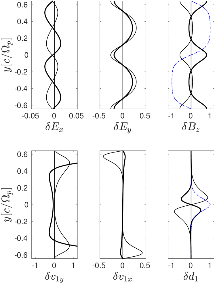
Figure 12: Transverse spatial structure of the eigenmode characterized by $\Gamma=0.13\,\Omega_{p}$, $k_{y}=k_{0}$ and $k_{x}=0.42\,\Omega_{p}/c$ (same parameters as in Fig. 9). The thick (resp. thin) solid lines plot the real (resp. imaginary) part of the eigenfunctions. The perturbed quantities are, from left to right and top to bottom, $\delta E_{x}$, $\delta E_{y}$, $\delta B_{z}$, normalized to $\mathrm{max}_{y}|\delta B_{z}|$ and $\delta v_{1x}$, $\delta v_{1y}$ and $\delta d_{1}$, normalized to $\mathrm{max}_{y}|\delta d_{1}|$. The thin dot-dashed lines plot the unperturbed quantities (normalized to their peak values).

For completeness, we construct in Figs. 13 and 14 synthetic 2D images of the two eigenmodes by adding, for both the total apparent density ($\sum_{\alpha}d_{\alpha}$) and the magnetic field ($B_{z}$), the zeroth and first order terms. The first order term is multiplied by a factor large enough to clearly illustrate the instability pattern. As expected, the dominant mode gives rise to in-phase oscillations of all filaments, and therefore to similar kinked deformations of $\sum_{\alpha}d_{\alpha}$ and $B_{z}$ (Fig. 13). For the sub-dominant mode (Fig. 14), the out-of-phase oscillations of adjacent current filaments translate into sausage-type magnetic fluctuations.

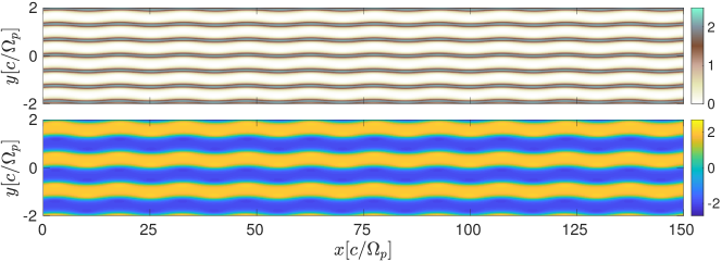
Figure 13: 2D spatial structure of the eigenmode characterized by $\Gamma=0.22\,\Omega_{p}$, $k_{y}=0$ and $k_{x}=0.42\,\Omega_{p}/c$. The unperturbed symmetric system is defined by $T_{0}=1$, $\gamma_{0}=10$ and $\xi=5$. Top panel: total particle density ($\sum_{\alpha}d_{\alpha}$). Bottom panel: transverse magnetic field ($B_{z}$).

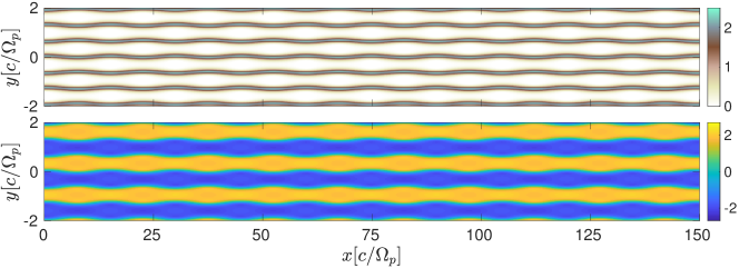
Figure 14: 2D spatial structure of the eigenmode characterized by $\Gamma=0.13\,\Omega_{p}$, $k_{y}=k_{0}$ and $k_{x}=0.42\,\Omega_{p}/c$ (same parameters as in Fig. 13). Top panel: total particle density ($\sum_{\alpha}d_{\alpha}$). Bottom panel: transverse magnetic field ($B_{z}$).

V.2 Transition from FMI to DKI

We now derive an analytic formula for the transition between dominant filament-merging and drift-kink instabilities in a symmetric relativistic filamentary system. To this goal, we seek an approximate expression for the relativistic DKI assuming negligible coupling effects between neighboring filaments. Our calculation, detailed in Appendix B, draws upon the approaches used in Refs. Pritchett_1996 ; Daughton_1999 ; Zenitani_2007 in the non- or weakly relativistic regimes. Here we only summarize its main steps and results.

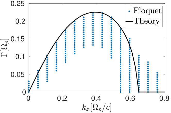
Figure 15: Growth rate of the relativistic drift kink instability as a function of $k_{x}$ for a two-beam filamentary system with $T_{0}=1$, $\gamma_{0}=10$, $a_{0}=1$ ($\xi=5$) and $\Gamma_{\rm ad}=4/3$. The results of the Floquet analysis are shown as blue points, while the solid black curve plots the analytic formula (48) for an isolated current filament.

Let us first consider a highly relativistic current filament, for which we assume

$$\bm{\beta}\cdot\delta\bm{\beta}=0\,,$$ (46)

in agreement with the spatial profiles of Fig. 11. Furthermore, we assume that the pressure balance condition is satisfied,

$$\frac{\mathbf{B}\cdot\delta{\mathbf{B}}}{4\pi}+\delta{p}_{+}+\delta{p}_{-}=0\,,$$ (47)

where $(+,-)$ refers to the charge of the two species making up the current filament. This condition is compatible with the profiles obtained from the Floquet theory. By substituting the above relations into the linearized two-fluid-Maxwell system, one can obtain the following expression for the DKI growth rate ($\Gamma_{\mathrm{DKI}}$) in a relativistic Harris-type current sheet:

$$h_{0}\frac{\Gamma^{2}_{\mathrm{DKI}}}{\Omega_{p}^{2}}\simeq\sqrt{1+4h_{0}\frac{k_{x}^{2}c^{2}}{\Omega_{p}^{2}}}-1-h_{0}\frac{k_{x}^{2}c^{2}}{\Omega_{p}^{2}}\,,$$ (48)

where $h_{0}=1+\frac{\Gamma_{\rm ad}}{\Gamma_{\rm ad}-1}T_{0}$. This formula predicts the maximum growth rate for the DKI

$$\Gamma_{\mathrm{DKI,max}}\simeq\frac{\Omega_{p}}{2\sqrt{h_{0}}}\,,$$ (49)

reached at $k_{x}=\sqrt{3/4h_{0}}\,\Omega_{p}/c$.

In Fig. 15, we compare Eq. (48) with the DKI growth rates computed numerically using the Floquet method for a strongly nonlinear periodic system defined by $T_{0}=1$, $\gamma_{0}=10$, $a_{0}=0.5$ ($\xi=5$) and $\Gamma_{\mathrm{ad}}=4/3$. For a given value of $k_{x}$, each blue point represents a solution to the Floquet problem. We observe that the analytic formula closely reproduces the upper envelope of the numerical growth rates, thus proving that inter-filament effects are indeed negligible in the (symmetric) strong-pinching regime.

In order to determine which instability (FMI or DKI) dominates a given symmetric system, one must compare the maximum growth rate of the DKI [Eq. (49)] with that of the FMI. An accurate formula for the latter should, in principle, account for the inhomogeneity of the unperturbed system, which is usually done via a truncated Floquet expansion Mishra_2014 . Here we opt for a much simpler approach, based on the observation that the FMI behaves similarly to the CFI in the very weakly nonlinear (or quasi homogeneous) limit (see Fig. 3). In Appendix C, the following expression for the ultra-relativistic limit of the maximum growth rate of the CFI is obtained

$$\Gamma_{\mathrm{CFI,max}}\simeq\frac{2\Omega_{p}}{\sqrt{h_{0}}}\exp(-\xi/2)\,.$$ (50)

Since the nonlinearity of the filaments tends to quell the FMI, this expression represents an upper bound value of the FMI growth rate.

According to Eqs. (49) and (50), the DKI is predicted to prevail over the FMI when the nonlinearity parameter exceeds the approximate threshold value

$$\xi_{\mathrm{th}}\simeq 4\,\log 2\simeq 2.7\,.$$ (51)

This analytic criterion for the FMI-DKI transition is in close agreement with our numerical results, which show a transition at $\xi\simeq 2.5$.

V.3 2D PIC simulation

We now present the results of a 2D3V calder simulation using the parameters considered in Sec. V.1 ($T_{0}=1$, $\gamma_{0}=10$, $a_{0}=0.5$). The domain size is $25000\,\Delta x\times 1000\,\Delta y$ with a discretization $\Delta x=\Delta y=\lambda_{0}/200=0.0064\,c/\Omega_{p}$. Each pinched filament extends over about 15 cells. These parameters allow us to resolve the $(k_{x},k_{y}$) Fourier space in the range $[0.04,976]\times[0.976,976]\,(\Omega_{p}/c)^{2}$. Each cell initially contains 10 macro-particles per species. The Maxwell equations are solved using the Cole-Karkkainen scheme Cole_1997a ; Cole_2002 ; Karkkainen_2006 , which enables us to use a large time step, $\Delta t=0.99\,\Delta x/c$. As usual, we apply periodic boundary conditions to both fields and particles.

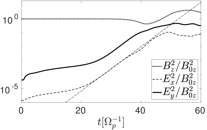
Figure 16: 2D PIC simulation with the parameters $T_{0}=1$, $\gamma_{0}=10$ and $a_{0}=0.5$: time evolution of the electromagnetic energies (spatially integrated and normalized to the initial magnetic energy). The $B_{z}$ energy is plotted as a dotted line, the $E_{x}$ energy as a dashed line and the $E_{y}$ energy as a thick solid line. The growth rate, $\Gamma_{\mathrm{PIC}}\simeq 0.18\,\Omega_{p}$ (thin dashed-dotted line), is measured from the $E_{y}$ curve over the time interval $25\leq t\leq 35\,\Omega_{p}^{-1}$.

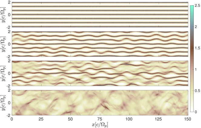
Figure 17: Simulated profiles of the total particle density (normalized to the initial peak density of the positrons) for the parameters of Fig. 16 at different times. From top to bottom: $t=7,\ 34,\ 39,\ 50\ \Omega_{p}^{-1}$.

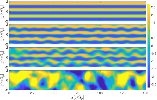
Figure 18: Simulated magnetic-field ($B_{z}$, normalized to $m\Omega_{p}/e$) profile for the parameters of Fig. 16 at different times. From top to bottom: $t=7,\ 34,\ 39,\ 50\ \Omega_{p}^{-1}$.

Figure 16 plots the time history of the electromagnetic energies, while Figs. 17 and 18 display, respectively, the maps of the magnetic field ($B_{z}$) and of the cold-beam-positron density ($d_{1}$) at times $t=7,\ 34,\ 39$ and $50\,\Omega_{p}^{-1}$. According to Fig. 16, the linear phase of the primary instability lasts until $t\simeq 40\,\Omega_{p}^{-1}$. During this period, the current filaments develop kink oscillations (Fig. 17). However, due to the broad unstable spectrum revealed in Fig. 9, they oscillate with a range of wavelengths and phases. While coherent motion between adjacent filaments can be seen locally, no single-mode pattern clearly emerges at the end of the linear phase. In like manner, the $B_{z}$ field distribution (Fig. 18) exhibits a mix of kink- and sausage-type perturbations instead of the globally coherent pattern displayed in Fig. 13.

As for the 1D FMI (Fig. 8), the 2D instability is first evidenced by exponentially growing electric-field energies (Fig. 16). An effective growth rate $\Gamma_{\mathrm{PIC}}\simeq 0.18\,\Omega_{p}$ is measured in the linear instability phase ($25\leq t\leq 35\,\Omega_{p}^{-1}$), comparable with the maximum theoretical value, $\Gamma_{\mathrm{max}}\simeq 0.22\,\Omega_{p}$. In agreement with the predicted structure of the dominant mode (Fig. 11), the $E_{y}$ energy is about an order of magnitude larger than the $E_{x}$ energy in the exponential phase. This feature starkly contrasts with the behavior of the 1D FMI treated in Sec. IV.2 (in the symmetric two-beam regime), for which the $E_{y}$ energy hardly grows (Fig. 8). Another major difference with the FMI is that the saturation of the DKI ($35\lesssim t\lesssim 40\,\Omega_{p}^{-1}$) goes along with a sudden drop in the total magnetic energy (to $\sim 43\%$ of its initial value). This magnetic-field dissipation is an expected effect of the DKI, which causes efficient particle heating Zenitani_2007 .

Once the initially strongly pinched filaments have been significantly distorted and smoothed out (see Figs. 17 and 18 at $t=39\,\Omega_{p}^{-1}$), a secondary instability of the CFI type is triggered by the residual momentum anisotropy of the plasma: this causes the magnetic energy to rebound again at $t\gtrsim 40\,\Omega_{p}^{-1}$, and rise until $t\simeq 50\,\Omega_{p}^{-1}$, at which time it seems to saturate. The bottom panel of Fig. 17 ($t=50\,\Omega_{p}^{-1}$) indicates that the plasma homogenization is then almost complete. Figure 18, however, shows that the transverse wavelength of the secondary CFI is typically the transverse domain size. A more precise description of the late-time nonlinear evolution of the system (which exceeds the scope of the present study) would therefore necessitate a larger simulation box.

VI 2D instability of asymmetric filaments

Finally, we address the interaction of a cold background plasma (indexed by ‘$p$’) with a counterstreaming hot beam (indexed by ‘$b$’), both composed of electrons and positrons. In asymmetric configurations, $\omega$ acquires a real part, which renders the Fourier space sampling complex. Moreover, not all frames are well defined for searching a purely real longitudinal wave number $k_{x}$. Here, this frame is chosen to be the so-called Weibel frame Pelletier_2018 , in which the electrostatic field of the stationary state vanishes. In the linear limit, this frame can be determined by setting $\phi_{0}=0$ in Eq. (14), which gives the following relation between the plasma species

$$\sum\limits_{\alpha}\frac{N_{\alpha}\beta_{\alpha 0}\gamma_{\alpha 0}^{2}}{T_{\alpha}}=0\,.$$ (52)

When $N_{p}/N_{b}\gg 1$, the Weibel frame tends to the rest frame of the cold background plasma Pelletier_2018 . In the following, we focus on a particular configuration defined by $T_{p0}=0.01$, $T_{b0}=1$, $\beta_{b0}=-0.9971$ ($\gamma_{b0}=13$), $\beta_{p0}=0.1672$, $\Gamma_{\rm ad,p}=5/3$, $\Gamma_{\rm ad,b}=4/3$ and $N_{p}/N_{b}=10$. The vector potential maximum is set to $a_{0}=0.05$, yielding $\xi_{p}\simeq 0.85$ and $\xi_{b}\simeq 0.66$, and hence moderately pinched current filaments, as confirmed by the equilibrium spatial profiles plotted in Fig. 19. The lab-frame is chosen such that the plasma parameters fulfill Eq. (52), leading to $|E_{0y}|\ll|B_{0z}|$ (see Fig. 19). The stationary system has a wavelength $\lambda_{0}\simeq 1.45\,c/\Omega_{p}$.

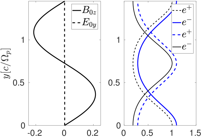
Figure 19: Stationary solution to the fluid-Maxwell equations in an $e^{-}e^{+}$ system composed of a hot beam ($T_{b0}=1$, $\beta_{b0}=-0.9971$) and a background cold plasma ($T_{p0}=0.01$, $\beta_{p0}=0.1672$, $N_{p}/N_{b}=10$). The vector potential maximum is $a_{0}=0.05$, resulting in a wavelength $\lambda_{0}=1.45\,c/\Omega_{p}$. Left panel: $B_{0z}(y)$ (solid line) and $E_{0y}(y)$ (dashed line), normalized to $\mathrm{max}_{y}B_{0z}$. Right panel: Density of the electrons (solid lines) and positrons (dashed lines) in the hot (blue) and cold (black) beams, normalized to the maximum cold-beam electron density.

VI.1 Floquet analysis

The Floquet analysis is carried out by setting, for each real value of $k_{x}$, an imaginary value ($\Gamma$) for $\omega$, and varying its real value ($\omega_{r}$) in order to find a vanishing value of $\Im k_{y}$. The roots are approached using a bisection method and computing the local derivative of $\Im k_{y}$. Figure 20 plots the $k_{y}$ dependence of $\Gamma$ for the longitudinal wavenumber ($k_{x}\simeq 0.95\,\Omega_{p}/c$) associated with the fastest-growing mode. In contrast to the symmetric configuration, two unstable branches are found: the upper one extends over the full fundamental zone ($0\leq k_{y}\leq k_{0}\simeq 4.3\,\Omega_{p}/c$), while the lower one is restricted to the range $0\leq k_{y}\leq 1.7\,\Omega_{p}/c$. The dominant mode pertains to the upper branch, and is characterized by a Floquet exponent $k_{y}\simeq 2.0\,\Omega_{p}/c$, a growth rate $\Gamma\simeq 0.16\,\Omega_{p}$ and a real frequency $\omega_{r}\simeq-0.75\,\Omega_{p}$ (Fig. 20). This mode differs significantly from the one governing the system in the homogeneous limit, which is characterized by $k_{x}\simeq 1.3\,\Omega_{p}/c$, $k_{y}\simeq 3.2\,\Omega_{p}/c$, $\Gamma\simeq 0.25\,\Omega_{p}$ and $\omega_{r}\simeq-1.1\,\Omega_{p}$.

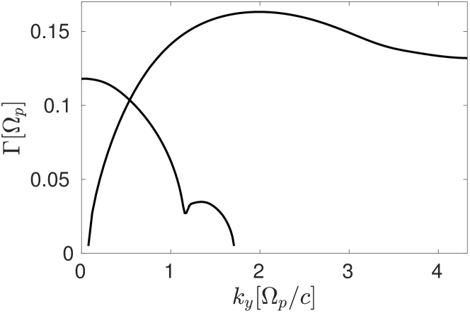
Figure 20: Instability growth rate ($\Gamma$) as a function of the Floquet exponent ($k_{y}$) at $k_{x}=0.95\,\Omega_{p}/c$ (corresponding to the fastest-growing mode). The unperturbed system is asymmetric with the parameters of Fig. 19. The fundamental wavenumber is $k_{0}\,\equiv\,2\pi/\lambda_{0}\,=\,4.33\,\Omega_{p}/c$.

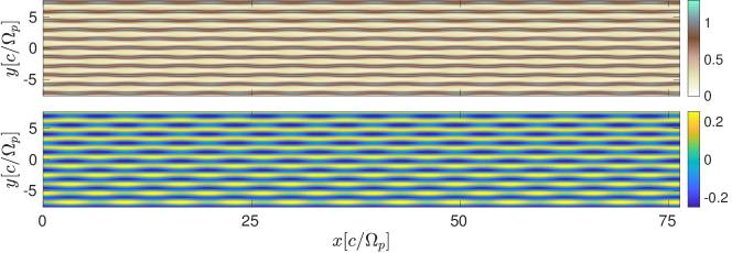
Figure 21: 2D spatial structure of the dominant eigenmodes ($k_{y}=\pm 2.0\,\Omega_{p}/c$) of the upper unstable branch shown in Fig. 20 normalized to the same amplitude. Top panel: apparent density of the cold-beam positrons ($d_{1}$). Bottom panel: transverse magnetic field ($B_{z}$). For each quantity, the zeroth and first order terms are added up.

Figure 21 displays the 2D structure of the dominant instability, as reflected by the apparent density of the cold-beam positrons ($d_{1}$) and the transverse magnetic field ($B_{z}$). For both quantities, the zeroth and first order terms are added up. The first order term is taken to be the sum of the eigenfunctions with $k_{y}=\pm 2.0\,\Omega_{p}/c$ and $k_{x}=0.95\,\Omega_{p}/c$ , which grow at the same rate and are initalized with the same amplitude. The structure that we observe differs from that found in the symmetric case (see Figs. 11 and 12): the filaments are subject to a mix of kink and bunching instabilities, with adjacent filaments of same species oscillating in opposite phase.

Figure 20 shows that the modes of the upper unstable branch in the range $1\lesssim k_{y}\lesssim k_{0}$ share similar growth rates ($\Gamma\sim 0.13-0.16\,\Omega_{p}$). In comparison, the lower branch presents a more localized maximum at $k_{y}=0$. The spatial structure of this sub-dominant mode corresponds to a bunching instability, as is the case for all lower-branch modes.

VI.2 2D PIC simulation

We have performed a 2D3V PIC simulation with the same initial parameters as the asymmetric Floquet problem. The numerical setup is that used in Sec. V.3, except that we now set $\Delta x=\Delta y=0.0292\,c/\Omega_{p}$. The time history of the electromagnetic energies is plotted in Fig. 23. From the evolution of the $E_{x}$ energy, the primary instability is estimated to grow at a rate $\Gamma_{\mathrm{PIC}}\simeq 0.14\,\Omega_{p}$, close to the theoretical prediction ($\Gamma_{\mathrm{max}}\simeq 0.16\,\Omega_{p}$). During this early phase, the total $B_{z}$ energy remains essentially constant. The exponential rise in the $E_{x}$ energy comes to an end at $t\simeq 40\,\Omega_{p}^{-1}$, at which time a new, slower-growing instability kicks in, giving rise to concomitant increases in the $E_{y}$ and $B_{z}$ energies.

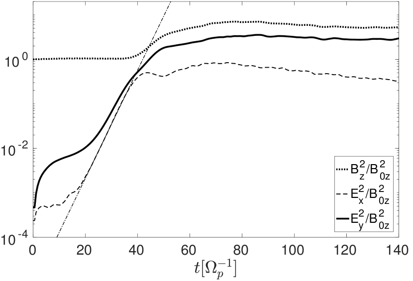
Figure 22: 2D PIC simulation with the parameters of Fig. 19: time evolution of the electromagnetic energies (spatially integrated and normalized to the initial magnetic energy). The $B_{z}$ energy is plotted as a dotted line, the $E_{x}$ energy as a dashed line and the $E_{y}$ energy as a thick solid line. The growth rate, $\Gamma_{\mathrm{PIC}}\simeq 0.14\,\Omega_{p}$ (thin dashed-dotted line), is measured from the $E_{x}$ curve over the time interval $20\leq t\leq 35\,\Omega_{p}^{-1}$.

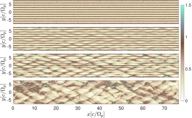
Figure 23: 2D PIC simulation with the parameters of Fig. 19: cold-beam positron density ($d_{1}$, normalized to its initial peak value) at different times. From top to bottom: $t=3,\ 32,\ 41,\ 58\ \Omega_{p}^{-1}$.

Figures 23 and 24 display the spatial structures of the cold-beam-positron density ($d_{1}$) and transverse magnetic field ($B_{z}$) at different times. The patterns observed at $t=32\,\Omega_{p}^{-1}$ (i.e., in the linear phase of the primary instability) consists of an ensemble of kink and bunching-type perturbations, as expected from the growth rate plateau of Fig. 20. At saturation ($t=41\,\Omega_{p}^{-1}$), the original 1D filamentary structure has evolved into a quasiperiodic pattern of compressed positron bunches, aligned along two preferential directions, tilted at angles $\simeq\pm 25^{\circ}$ relative to the flow axis. These angles are close to those characterizing the dominant Floquet eigenmode ($\tan^{-1}\left(k_{x}/k_{y}\right)\simeq\pm 25.4^{\circ}$). As time increases, these density islands tend to coalesce, giving rise to oblique modulations with increasing wavelength and tilted at larger angles ($\simeq\pm 35^{\circ}$, see panels at $t=58\,\Omega_{p}^{-1}$). Such unstable skew modes are reminiscent of the oblique instability arising in homogeneous asymmetric two-stream systems Bret_2010a .

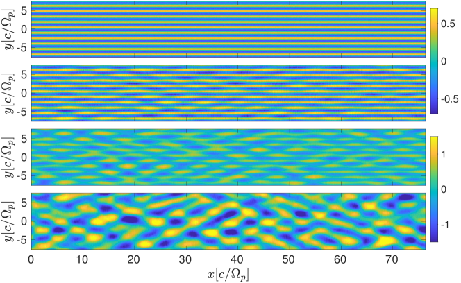
Figure 24: 2D PIC simulation with the parameters of Fig. 21: transverse magnetic field ($B_{z}$, normalized to $m\Omega_{p}/e$) at different times. From top to bottom: $t=3,\ 32,\ 41,\ 58\ \Omega_{p}^{-1}$.

VII Conclusion

To conclude, the stability of a periodic system of relativistic $e^{-}e^{+}$ current filaments, such as resulting from the current filamentation instability (CFI), has been thoroughly examined in a warm-fluid framework. As the nonlinearity of the equilibrium filaments (quantified by the dimensionless parameter $\xi_{\alpha}=\gamma_{\alpha}\left|\beta_{\alpha}\right|a_{0}/T_{\alpha}$) is increased, our numerical Floquet-type calculations predict a smooth transition from a dominant, purely transverse, filament merging instability (FMI) to a relatively long-wavelength drift-kink instability (DKI). In a weakly nonlinear, symmetric configuration ($\xi_{\alpha}=\xi$), the FMI is found to obey a dispersion relation close to that of the homogeneous CFI. As $\xi$ is raised, the FMI is progressively mitigated, and is eventually overtaken by DKI modes when $\xi\gtrsim 2.5$. In the strongly nonlinear limit, the filaments are well described by the relativistic Harris solution and behave essentially independently from one another. As a result, the dominant DKI modes share the periodicity of the unperturbed system, and their properties are similar to those analytically derived for a single isolated filament. We have briefly studied the stability of an asymmetric configuration composed of a hot beam streaming against a cold background plasma. The dominant primary mode consists of a combination of kink and bunching-type perturbations. A PIC simulation shows that this mode nonlinearly evolves into two oblique strings of high-density islands. Their subsequent decay is followed by the development of a larger-scale oblique instability, similar to that arising in homogeneous multi-stream plasmas. This scenario may be relevant to the precursor region of Weibel-mediated relativistic shocks Keshet_2008 where similarly asymmetric two-beam interactions are expected to arise.

For all the studied cases, the theoretical predictions are consistent with the results of PIC simulations. Our study, however, was limited to 1D and 2D systems. Extending it to a 3D geometry is not straightforward, both as regards the construction of the initial, 2D periodic array of nonlinear filaments and the numerical resolution of the 3D eigenmodes, to which the technique developed in the present work is ill-suited. Finally, we have restricted our analysis to relativistic pair plasmas: its generalization to electron-ion plasmas will be the subject of a forthcoming study.

Appendix A Linearized relativistic four-fluid equations

In this section, we present the full set of fluid equations used to obtain the Floquet-type eigenmodes of a periodic chain of current filaments. We consider a 2D $(x,y)$ system made up of four plasma fluids (two electron species and two positron species), initially flowing in the $x$ direction. The unperturbed system is a stationary, $y$-dependent solution to the fluid-Maxwell equations. In the linearized version of Eqs. (1)-(5), one can therefore use the simplifications $\partial_{t}\to-i\omega$ and $\partial_{x}\to ik_{x}$. The perturbed quantities are defined such that $p_{\alpha}=p_{\alpha 0}\left[f_{\alpha}(y)+\delta P_{\alpha}\right]$, $d_{\alpha}=d_{\alpha 0}\left[f_{\alpha}(y)+\delta D_{\alpha}\right]$, $\mathbf{v}_{\alpha}=\beta_{\alpha 0}c\left[\epsilon_{\alpha}\mathbf{1}_{x}+\delta\mathbf{V}_{\alpha}\right]$, $\mathbf{E}=E_{0y}f_{E}(y)\bm{1}_{y}+B_{0z}\delta\mathbf{e}$ and $B_{z}=B_{0z}\left[f_{B}(y)+\delta b_{z}\right]$. For each species $\alpha$, we have introduced $\beta_{\alpha 0}$ the absolute value of its unperturbed normalized velocity, $\epsilon_{\alpha}=\{1,-1,-1,1\}$ its drifting direction. The equilibrium density ($f_{\alpha}$), magnetic ($f_{B}$) and electric ($f_{E}$) profiles are computed numerically from Eqs. (12)-(14). The linearized equations read

$$\partial_{y}\delta e_{x} =-\frac{i\omega}{c}\delta b_{z}+ik_{x}\delta e_{y}\,,$$ (53)

$$\partial_{y}\delta b_{z} =-\frac{i\omega}{c}\delta e_{x}+\frac{4\pi}{B_{0z}}\sum\limits_{\alpha}q_{\alpha}\beta_{\alpha 0}d_{\alpha 0}\left[f_{\alpha}(y)\delta V_{\alpha x}+\epsilon_{\alpha}\delta D_{\alpha}\right]\,,$$ (54)

$$\partial_{y}\delta P_{\alpha} =\frac{q_{\alpha}d_{\alpha 0}B_{0z}}{p_{\alpha 0}}\left\{-\epsilon_{\alpha}f_{B}(y)\beta_{\alpha 0}\delta D_{\alpha}+f_{\alpha}(y)\delta e_{y}+\frac{E_{0y}}{B_{0z}}f_{E}(y)\delta D_{\alpha}+f_{\alpha}(y)\beta_{\alpha 0}\left[-\epsilon_{\alpha}\delta b_{z}-f_{B}(y)\delta V_{\alpha x}\right]\right\}\,$$

$$-\frac{\gamma_{\alpha}^{2}}{c^{2}}\frac{1}{p_{\alpha 0}}\left(p_{\alpha 0}\frac{\Gamma_{\rm ad,\alpha}}{\Gamma_{\rm ad,\alpha}-1}+\frac{d_{\alpha 0}}{\gamma_{\alpha}}mc^{2}\right)f_{\alpha}(y)\beta_{\alpha}c(-i\omega\delta V_{\alpha y}+\epsilon_{\alpha}\beta_{\alpha}c\ ik_{x}\delta V_{\alpha y})\,,$$ (55)

$$\partial_{y}\delta V_{\alpha y} =\frac{i\omega}{c\beta_{\alpha}f_{\alpha}(y)}\delta D_{\alpha}-ik_{x}\delta V_{\alpha x}-\frac{\partial_{y}f_{\alpha}(y)}{f_{\alpha}(y)}\delta V_{\alpha y}-\frac{ik_{x}\epsilon_{\alpha}}{f_{\alpha}(y)}\delta D_{\alpha}\,,$$ (56)

where the perturbed quantities $\delta e_{y}$, $\delta V_{\alpha x}$ and $\delta D_{\alpha}$ are given by

$$\delta e_{y} =-\frac{i}{\omega}\left[\frac{4\pi c}{B_{0z}}\sum\limits_{\alpha}q_{\alpha}\beta_{\alpha 0}d_{\alpha 0}f_{\alpha}(y)\delta V_{\alpha y}+ik_{x}c\delta b_{z}\right]\,,$$ (57)

$$\delta V_{\alpha x} =\frac{1}{\frac{\gamma_{\alpha}^{2}}{c^{2}}(p_{\alpha 0}\frac{\Gamma_{\rm ad,\alpha}}{\Gamma_{\rm ad,\alpha}-1}+\frac{d_{\alpha 0}}{\gamma_{\alpha}}mc^{2})f_{\alpha}(y)\beta_{\alpha 0}c\left(-i\omega+i\epsilon_{\alpha}\beta_{\alpha 0}ck_{x}\right)}\Biggl{\{}-ik_{x}p_{\alpha 0}\delta P_{\alpha}+q_{\alpha}d_{\alpha 0}B_{0z}\Bigl{[}f_{\alpha}(y)\delta e_{x}\Bigr{.}\Biggr{.}$$

$$\Biggl{.}\Bigl{.}+\beta_{\alpha 0}f_{\alpha}(y)f_{B}(y)\delta V_{y,\alpha}\Bigl{]}-\Bigl{[}q_{\alpha}\beta_{\alpha 0}^{2}d_{\alpha 0}B_{0z}f_{\alpha}(y)\delta e_{x}+\epsilon_{\alpha}q_{\alpha}\beta_{\alpha 0}^{2}d_{\alpha 0}E_{0y}f_{\alpha}(y)f_{E}(y)\delta V_{\alpha y}-i\epsilon_{\alpha}\omega c^{-1}p_{\alpha 0}\beta_{\alpha 0}\delta P_{\alpha}\Bigr{]}\Biggr{\}}\,,$$ (58)

$$\delta D_{\alpha} =\frac{1}{\Gamma_{\rm ad,\alpha}}\left[\delta P_{\alpha}+\epsilon_{\alpha}\Gamma_{\rm ad,\alpha}f_{\alpha}(y)\frac{\beta_{\alpha 0}^{2}}{1-\beta_{\alpha 0}^{2}}\delta V_{\alpha x}\right]\,.$$ (59)

We can avoid the numerical estimation of $\partial_{y}f_{\alpha}$ in Eq. (56) through the momentum equation in stationary state:

$$\frac{\partial_{y}f_{\alpha}(y)}{f_{\alpha}(y)}=q_{\alpha}\frac{d_{\alpha 0}}{p_{\alpha 0}}\left[E_{0y}f_{E}(y)-\beta_{\alpha 0x}B_{0z}f_{B}(y)\right]\,.$$ (60)

The system is solved using the Floquet theory for different points $(\omega,k_{x})\in\mathbb{C}\times\mathbb{R}^{+}$, giving the corresponding characteristic Floquet exponent $k_{y}$. We are interested in temporally unstable solutions, and hence we only retain the solutions with $k_{y}\in\mathbb{R}$.

Appendix B Analytic solution of the relativistic drift kink instability

In the strongly nonlinear (pinched) regime, each current filament can be described by an isolated system of two counterstreaming electron and positron fluids. In the following we derive an approximate analytic solution to the relativistic drift-kink instability (DKI), valid in the vicinity of the filament center. Our calculation is restricted to the case of two symmetric fluids. The positrons (resp. electrons) are taken to have a positive (resp. negative) velocity.

The set of equations is composed of the momentum, continuity and Maxwell’s equations, closed by an adiabatic equation of state:

$$\gamma^{2}_{\alpha}\left(p_{\alpha}+\epsilon_{\alpha}\right)\left(\partial_{ct}+\bm{\beta}_{\alpha}\cdot\bm{\nabla}\right)\bm{\beta}_{\alpha}=-\bm{\nabla}p_{\alpha}$$

$$+q_{\alpha}d_{\alpha}\left(\mathbf{E}+\bm{\beta}_{\alpha}\times\mathbf{B}\right)-\bm{\beta}_{\alpha}\left(q_{\alpha}d_{\alpha}\mathbf{E}\cdot\bm{\beta}_{\alpha}+\partial_{ct}p_{\alpha}\right)\,,$$ (61)

$$\bm{\nabla}\times\mathbf{B}=4\pi e\bm{\beta}\left(d_{+}+d_{-}\right)+\partial_{ct}\mathbf{E}\,,$$ (62)

$$\bm{\nabla}\cdot\mathbf{E}=4\pi e\left(d_{+}-d_{-}\right)\,,$$ (63)

$$\bm{\nabla}\times\mathbf{E}=-\partial_{ct}\mathbf{B}\,,$$ (64)

$$\delta\left(\frac{p_{\alpha}\gamma^{\Gamma_{\rm ad}}}{d^{\Gamma_{\rm ad}}_{\alpha}}\right)=0\,,$$ (65)

where $e$ is the elementary charge, $\bm{\beta}$ is the drifting velocity vector of the positron, $\beta=|\bm{\beta}|$, $\Gamma_{\rm ad}$ is the polytropic index and $\alpha=\left(+,-\right)$ refers to positrons and electrons. We expand all fluid quantities to first order (for a generic variable $b\,=\,b_{0}+\delta{b}$), and we introduce the following quantities:

$$\delta{b}^{+} =\delta{b}_{+}+\delta{b}_{-}\,,$$ (66)

$$\delta{b}^{-} =\delta{b}_{+}-\delta{b}_{-}\,.$$ (67)

For the sake of tractability, we make use of two assumptions. Firstly, we assume a purely transverse velocity perturbation,

$$\bm{\beta}_{0}\cdot\delta\bm{\beta}=0\,.$$ (68)

Secondly, we assume that the pressure balance condition in the filament is fulfilled:

$$\frac{\mathbf{B}_{0}\cdot\delta{\mathbf{B}}}{4\pi}+\delta p^{+}=0\,.$$ (69)

Using these two relations, the sum and difference of the linearized momentum equations take the following form

$$M_{0}\left(-i\omega\delta{\bm{\beta}}^{+}+\beta_{0}ik_{x}\delta\bm{\beta}^{-}\right)=-\nabla\left(\delta p^{+}\right)-ed_{0}\mathbf{B}_{0}\times\delta\bm{\beta}^{-}+2ed_{0}\bm{\beta}_{0}\times\delta\mathbf{B}-e\mathbf{B}_{0}\times\bm{\beta}_{0}\delta d^{+}+i\omega\bm{\beta}_{0}\delta p^{-}\,,$$ (70)

$$M_{0}\left(-i\omega\delta\bm{\beta}^{-}+\beta_{0}ik_{x}\delta\bm{\beta}^{+}\right)=-\nabla\left(\delta p^{-}\right)+2ed_{0}\delta\mathbf{E}-ed_{0}\mathbf{B}_{0}\times\delta\bm{\beta}^{+}-e\mathbf{B}_{0}\times\bm{\beta}_{0}\delta d^{-}-2e\bm{\beta}_{0}d_{0}\bm{\beta}_{0}\cdot\delta\mathbf{E}+i\omega\bm{\beta}_{0}\delta p^{+}\,,$$ (71)

where

$$M_{0}=\gamma_{0}^{2}\left(\frac{\Gamma_{\mathrm{ad}}}{\Gamma_{\mathrm{ad}}-1}p_{0}+n_{0}mc^{2}\right)\,.$$ (72)

Projecting Eqs. (70) and (71) along the $x$ axis gives

$$-ik_{x}\delta p^{\pm}+i\omega\ \delta p^{\mp}+ed_{0}B_{0}\delta\beta_{y}^{\mp}=0\,.$$ (73)

Moreover, the linearized continuity equation writes

$$-i\omega\ \delta d^{\pm}+ik_{x}\delta d^{\mp}+\partial_{y}d_{0}\delta\beta^{\pm}_{y}+d_{0}\partial_{y}\delta\beta^{\pm}_{y}=0\,.$$ (74)

The adiabatic closure condition relates the perturbed pressure and density as

$$\delta p^{\pm}=\Gamma_{\mathrm{ad}}\frac{p_{0}}{d_{0}}\delta d^{\pm}\,.$$ (75)

Combining the previous equations leads to the differential equation fulfilled by $\delta{\beta}^{\pm}_{y}$:

$$\left(\Gamma_{\mathrm{ad}}\partial_{y}\log d_{0}+ed_{0}B_{0}\right)\delta\beta^{\pm}_{y}+\Gamma_{\mathrm{ad}}p_{0}\partial_{y}\delta\beta^{\pm}_{y}=0\,.$$ (76)

We assume that the current filament initially obeys the Harris solution,

$$d_{0} =\gamma_{0}n_{0}\cosh^{-2}\left(y/l\right)\,,$$ (77)

$$B_{0} =\sqrt{16\pi n_{0}T_{0}}\tanh\left(y/l\right)\,,$$ (78)

with the characteristic width [Eq. (26)]

$$l=\frac{\sqrt{T_{0}}}{\gamma_{0}}\frac{c}{\Omega_{p}}\,.$$ (79)

In the Harris equilibrium, the solution to Eq. (76) is

$$\delta{\beta}^{\pm}_{y}=\delta{\beta}^{\pm}_{y}\left(0\right)\cosh\left(y/l\right)^{2-2/\Gamma_{\rm ad}}\,.$$ (80)

This solution is even in $y$, consistent with the DKI. The validity of this expression is limited to the inner region of the current filament.

Linearizing the cross product of $\bm{B}$ with Eq. (62), one obtains

$$-e\mathbf{B}_{0}\times\bm{\beta_{0}}\delta{d}^{+}+2ed_{0}\bm{\beta}_{0}\times\delta\mathbf{B}+ed_{0}\delta\bm{\beta}^{-}\times\mathbf{B}_{0}$$

$$=-\nabla\left(\frac{\mathbf{B}_{0}\cdot\delta\mathbf{B}}{4\pi}\right)-\frac{i\omega}{4\pi}\mathbf{B}_{0}\times\delta\mathbf{E}\,.$$ (81)

The drift term $\frac{i\omega}{4\pi}\mathbf{B}_{0}\times\delta\mathbf{E}$ is found to be negligible. Substituting Eq. (B) into Eq. (70) gives

$$M_{0}\left(-i\omega\delta{\bm{\beta}}^{+}+\beta_{0}ik_{x}\delta{\bm{\beta}}^{-}\right)=i\omega\bm{\beta}_{0}\delta{p}^{-}\,.$$ (82)

Therefore, $\delta{p}^{-}$ is of the same order as the $\delta\beta^{\pm}_{x}$ terms, and hence can be neglected (in agreement with the numerical Floquet solutions). The projection of the two latter equations along the $y$-axis leads to the following system

$$M_{0}\left(-i\omega\delta\beta^{+}_{y}+\beta_{0}ik_{x}\delta\beta^{-}_{y}\right) =0\,,$$ (83)

$$M_{0}\left(-i\omega\delta\beta^{-}_{y}+\beta_{0}ik_{x}\delta\beta^{+}_{y}\right) =2ed_{0}\delta E_{y}\,.$$ (84)

The perturbed transverse electric field, $\delta E_{y}$, is related to $\delta\beta^{\pm}_{y}$ through

$$\delta E_{y}=\frac{4\pi}{i\omega B_{0}}\left(eB_{0}\delta\beta^{-}_{y}-ik_{x}\delta p^{+}\right)\,.$$ (85)

Combining (83)-(85) and evaluating the resulting system at the filament center finally gives

$$\frac{\omega^{2}}{k_{x}^{2}}\left\{2+\left[\frac{k_{x}^{2}}{\Omega_{p}^{2}}-\frac{\omega^{2}}{\Omega_{p}^{2}}\right]-\Gamma_{\rm ad}\left[2+\left(\frac{k_{x}^{2}}{\Omega_{p}^{2}}-\frac{\omega^{2}}{\Omega_{p}^{2}}\right)\left(1+T\right)\right]\right\}$$

$$+2-\left[\frac{k_{x}^{2}}{\Omega_{p}^{2}}-\frac{\omega^{2}}{\Omega_{p}^{2}}\right]-\Gamma_{\rm ad}\left[2-\left(\frac{k_{x}^{2}}{\Omega_{p}^{2}}-\frac{\omega^{2}}{\Omega_{p}^{2}}\right)\left(1+T\right)\right]=0\,.$$ (86)

The dispersion relation of the DKI therefore writes

$$h_{0}\frac{\Gamma^{2}}{\Omega_{p}^{2}}=\sqrt{1+4h_{0}\frac{k_{x}^{2}}{\Omega_{p}^{2}}}-1-h_{0}\frac{k_{x}^{2}}{\Omega_{p}^{2}}\,,$$ (87)

where

$$h_{0}=1+\frac{\Gamma_{\mathrm{ad}}}{\Gamma_{\mathrm{ad}}-1}T_{0}\,.$$ (88)

The growth rate reaches a maximum value of

$$\Gamma_{\mathrm{DKI,max}}=\frac{1}{2}\frac{\Omega_{p}}{\sqrt{h_{0}}}$$ (89)

for $k_{x}=(\sqrt{3}/2)\Omega_{p}/\sqrt{h_{0}}$.

Appendix C Analytic solution of the current filamentation instability

The dispersion relation of the CFI in a system composed of two symmetric, relativistic pair plasma flows is obtained by linearizing Eqs. (1)-(5) in the limit of vanishing fields. This yields the following linear system

$$\begin{pmatrix}-i\tilde{k}_{y}&\tilde{\Gamma}&0&0&0&0\\ \tilde{\Gamma}+\frac{2}{h_{0}\tilde{\Gamma}}&-i\tilde{k}_{y}&\frac{\beta_{0}\gamma_{0}(h_{0}-\Gamma_{\rm ad}T_{0})}{\Gamma_{\rm ad}h_{0}}&-\frac{\beta_{0}\gamma_{0}(h_{0}-\Gamma_{\rm ad}T_{0})}{\Gamma_{\rm ad}h_{0}}&0&0\\ 0&-\frac{\beta_{0}\gamma_{0}}{T_{0}}&-i\tilde{k}_{y}&0&-\frac{\beta_{0}\gamma_{0}^{2}\left(h_{0}\tilde{\Gamma}^{2}+1\right)}{T\tilde{\Gamma}}&-\frac{\beta_{0}\gamma_{0}^{2}}{T_{0}\tilde{\Gamma}}\\ 0&\frac{\beta_{0}\gamma_{0}}{T_{0}}&0&-i\tilde{k}_{y}&-\frac{\beta_{0}\gamma_{0}^{2}}{T_{0}\tilde{\Gamma}}&-\frac{\beta_{0}\gamma_{0}^{2}\left(h_{0}\tilde{\Gamma}^{2}+1\right)}{T_{0}\tilde{\Gamma}}\\ -\frac{1}{\gamma_{0}h_{0}}&0&\frac{\beta_{0}T_{0}\tilde{\Gamma}}{h_{0}}-\frac{\tilde{\Gamma}}{\beta_{0}\Gamma_{\rm ad}}&0&-i\tilde{k}_{y}&0\\ \frac{1}{\tilde{\Gamma}h_{0}}&0&0&\frac{\beta_{0}T_{0}\tilde{\Gamma}}{h_{0}}-\frac{\tilde{\Gamma}}{\beta_{0}\Gamma_{\rm ad}}&0&-i\tilde{k}_{y}\\ \end{pmatrix}\cdot\begin{pmatrix}\delta e_{x}\\ \delta b_{z}\\ \delta p_{+}\\ \delta p_{-}\\ \delta v_{y+}\\ \delta v_{y-}\end{pmatrix}=0\,,$$ (90)

where we have introduced

$$\omega_{p}=\Omega_{p}\,e^{-\gamma_{0}a_{0}/2T_{0}}\,,$$ (91)

$$\tilde{\Gamma}=\Gamma/\omega_{p}\,,$$ (92)

$$\tilde{k}_{y}=k_{y}c/\omega_{p}\,,$$ (93)

and $h_{0}$ is given by Eq. (88). To leading order in $1/\gamma_{0}^{2}$ , the dispersion relation writes

$$h_{0}\tilde{\Gamma}^{2}=\frac{1}{2}\left(\sqrt{1+16/K_{y}^{2}}-1\right)K_{y}^{2}-\frac{1}{2\gamma_{0}^{2}\left(h_{0}-\Gamma_{\mathrm{ad}}T_{0}\right)}\left[4h_{0}+\Gamma_{\mathrm{ad}}T_{0}K_{y}^{2}+\frac{4h_{0}+\left(8+K_{y}^{2}\right)\Gamma_{\mathrm{ad}}T_{0}}{\sqrt{1+16/K_{y}^{2}}}\right]\,,$$ (94)

with $K_{y}=\sqrt{h_{0}}\tilde{k}_{y}$. In the ultrarelativistic case ($\gamma_{0}\to\infty$), the maximum growth rate is

$$\Gamma_{\mathrm{CFI,max}}=\frac{2}{\sqrt{h}}\omega_{p}=\frac{2}{\sqrt{h}}e^{-\gamma_{0}a_{0}/2T_{0}}\Omega_{p}\,.$$ (95)

References

- [1] E. S. Weibel. Spontaneously Growing Transverse Waves in a Plasma Due to an Anisotropic Velocity Distribution. Phys. Rev. Lett., 2:83–84, Feb 1959.
- [2] R. C. Davidson, D. A. Hammer, I. Haber, and C. E. Wagner. Nonlinear Development of Electromagnetic Instabilities in Anisotropic Plasmas. Phys. Fluids, 15(2):317–333, 1972.
- [3] B. D. Fried. Mechanism for Instability of Transverse Plasma Waves. Phys. Fluids, 2:337, Mar 1959.
- [4] F. Califano, F. Pegoraro, and S. V. Bulanov. Spatial structure and time evolution of the Weibel instability in collisionless inhomogeneous plasmas. Phys. Rev. E, 56:963–969, Jul 1997.
- [5] R. Lee and M. Lampe. Electromagnetic instabilities, filamentation, and focusing of relativistic electron beams. Phys. Rev. Lett., 31:1390–1393, Dec 1973.
- [6] M. Honda, J. Meyer-ter Vehn, and A. Pukhov. Collective stopping and ion heating in relativistic-electron-beam transport for fast ignition. Phys. Rev. Lett., 85:2128–2131, Sep 2000.
- [7] M. Gedalin, M. A. Balikhin, and D. Eichler. Efficient electron heating in relativistic shocks and gamma-ray-burst afterglow. Phys. Rev. E, 77:026403, Feb 2008.
- [8] S. S. Moiseev and R. Z. Sagdeev. Collisionless shock waves in a plasma in a weak magnetic field. Journal of Nuclear Energy. Part C, Plasma Physics, Accelerators, Thermonuclear Research, 5(1):43, 1963.
- [9] M. V. Medvedev and A. Loeb. Generation of Magnetic Fields in the Relativistic Shock of Gamma-Ray Burst Sources. Astrophys. J. , 526:697–706, December 1999.
- [10] M. Lemoine and G. Pelletier. Dispersion and thermal effects on electromagnetic instabilities in the precursor of relativistic shocks. Mon. Not. Roy. Astron. Soc., 417:1148–1161, Oct 2011.
- [11] G. Pelletier, A. Bykov, D. Ellison, and M. Lemoine. Towards Understanding the Physics of Collisionless Relativistic Shocks. Space Science Reviews, 207:319–360, jul 2017.
- [12] J. T. Frederiksen, C. B. Hededal, T. Haugbølle, and Å. Nordlund. Magnetic field generation in collisionless shocks: Pattern growth and transport. Astrophys. J. Lett., 608(1):L13, 2004.
- [13] T. N. Kato. Relativistic collisionless shocks in unmagnetized electron-positron plasmas. Astrophys. J., 668(2):974, 2007.
- [14] A. Spitkovsky. Particle Acceleration in Relativistic Collisionless Shocks: Fermi Process at Last? Astrophys. J. Lett., 682:L5, Jul 2008.
- [15] U. Keshet, B. Katz, A. Spitkovsky, and E. Waxman. Magnetic field evolution in relativistic unmagnetized collisionless shocks. Astrophys. J., 693:L127–L130, 2009.
- [16] S. F. Martins, R. A. Fonseca, L. O. Silva, and W. B. Mori. Ion dynamics and acceleration in relativistic shocks. Astrophy. J. Lett., 695(2):L189, 2009.
- [17] K.-I. Nishikawa, J. Niemiec, P. E. Hardee, M. Medvedev, H. Sol, Y. Mizuno, B. Zhang, M. Pohl, M. Oka, and D. H. Hartmann. Weibel instability and associated strong fields in a fully three-dimensional simulation of a relativistic shock. Astrophys. J. Lett., 698(1):L10, 2009.
- [18] L. Sironi, A. Spitkovsky, and J. Arons. The Maximum Energy of Accelerated Particles in Relativistic Collisionless Shocks. Astrophys. J., 771:54, Jul 2013.
- [19] K. Ardaneh, D. Cai, K.-I. Nishikawa, and B. Lembége. Collisionless Weibel Shocks and Electron Acceleration in Gamma-Ray Bursts. Astrophys. J. , 811:57, Sep 2015.
- [20] L.Sironi and A. Spitkovsky. Synthetic Spectra from Particle-In-Cell Simulations of Relativistic Collisionless Shocks. Astrophys. J. Lett., 707(1):L92, 2009.
- [21] T. Frederiksen, J. T.and Haugbølle, M. V. Medvedev, and Å. Nordlund. Radiation spectral synthesis of relativistic filamentation. Astrophys. J. Lett., 722(1):L114, 2010.
- [22] Brett D. Keenan and Mikhail V. Medvedev. Particle transport and radiation production in sub-larmor-scale electromagnetic turbulence. Phys. Rev. E, 88:013103, Jul 2013.
- [23] M. Swisdak, Yi-Hsin Liu, and J. F. Drake. Development of a turbulent outflow during electron-positron magnetic reconnection. Astrophys. J., 680(2):999, 2008.
- [24] Kim Molvig. Filamentary instability of a relativistic electron beam. Phys. Rev. Lett., 35:1504–1507, Dec 1975.
- [25] H. Lee and L. E. Thode. Electromagnetic two-stream and filamentation instabilities for a relativistic beam-plasma system. The Physics of Fluids, 26(9):2707–2716, 1983.
- [26] B. Allen, V. Yakimenko, M. Babzien, M. Fedurin, K. Kusche, and P. Muggli. Experimental study of current filamentation instability. Phys. Rev. Lett., 109:185007, Nov 2012.
- [27] A. Ramani and G. Laval. Heat flux reduction by electromagnetic instabilities. Phys. Fluids, 21:980–991, June 1978.
- [28] M. A. True. Weibel instability in the spherical corona of a laser fusion target. The Physics of Fluids, 28(8):2597–2601, 1985.
- [29] E. M. Epperlein, T. H. Kho, and M. G. Haines. The collisional Weibel Instability of a laser heated plasma slab. Plasma Phys. Control. Fus., 28(1B):393, 1986.
- [30] P. E. Masson-Laborde, W. Rozmus, Z. Peng, D. Pesme, S. Hüller, M. Casanova, V. Yu. Bychenkov, T. Chapman, and P. Loiseau. Evolution of the stimulated Raman scattering instability in two-dimensional particle-in-cell simulations. Phys. Plasmas, 17(9):092704, 2010.
- [31] H. Ruhl. 3D kinetic simulation of super-intense laser-induced anomalous transport. Plasma Sources Science Technology, 11(27):A154–A158, August 2002.
- [32] Y. Sentoku, K. Mima, P. Kaw, and K. Nishikawa. Anomalous Resistivity Resulting from MeV-Electron Transport in Overdense Plasma. Phys. Rev. Lett., 90:155001, Apr 2003.
- [33] M. Tatarakis, F. N. Beg, E. L. Clark, A. E. Dangor, R. D. Edwards, R. G. Evans, T. J. Goldsack, K. W. Ledingham, P. A. Norreys, M. A. Sinclair, M.-S. Wei, M. Zepf, and K. Krushelnick. Propagation Instabilities of High-Intensity Laser-Produced Electron Beams. Phys. Rev. Lett., 90(17):175001, April 2003.
- [34] M. S. Wei, F. N. Beg, E. L. Clark, A. E. Dangor, R. G. Evans, A. Gopal, K. W. D. Ledingham, P. McKenna, P. A. Norreys, M. Tatarakis, M. Zepf, and K. Krushelnick. Observations of the filamentation of high-intensity laser-produced electron beams. Phys. Rev. E, 70:056412, Nov 2004.
- [35] J. C. Adam, A. Héron, and G. Laval. Dispersion and transport of energetic particles due to the interaction of intense laser pulses with overdense plasmas. Phys. Rev. Lett., 97:205006, Nov 2006.
- [36] A. Debayle, J. J. Honrubia, E. d’Humières, and V. T. Tikhonchuk. Divergence of laser-driven relativistic electron beams. Phys. Rev. E, 82:036405, Sep 2010.
- [37] S. Mondal, V. Narayanan, W. J. Ding, A. D. Lad, B. Hao, S. Ahmad, W. M. Wang, Z. M. Sheng, S. Sengupta, P. Kaw, A. Das, and G. R. Kumar. Direct observation of turbulent magnetic fields in hot, dense laser produced plasmas. Proceedings of the National Academy of Science, 109:8011–8015, May 2012.
- [38] K. Quinn, L. Romagnani, B. Ramakrishna, G. Sarri, M. E. Dieckmann, P. A. Wilson, J. Fuchs, L. Lancia, A. Pipahl, T. Toncian, O. Willi, R. J. Clarke, M. Notley, A. Macchi, and M. Borghesi. Weibel-induced filamentation during an ultrafast laser-driven plasma expansion. Phys. Rev. Lett., 108:135001, Mar 2012.
- [39] M. Tabak, J. Hammer, M. E. Glinsky, W. L. Kruer, S. C. Wilks, J. Woodworth, E. M. Campbell, and M. D. Perry. Ignition and high gain with ultrapowerful lasers. Phys. Plasmas, 1:1626, Jan 1994.
- [40] A.P.L. Robinson, D.J. Strozzi, J.R. Davies, L. Gremillet, J.J. Honrubia, T. Johzaki, R.J. Kingham, M. Sherlock, and A.A. Solodov. Theory of fast electron transport for fast ignition. Nuclear Fusion, 54(5):054003, 2014.
- [41] S. Göde, C. Rödel, K. Zeil, R. Mishra, M. Gauthier, F.-E. Brack, T. Kluge, M. J. MacDonald, J. Metzkes, L. Obst, M. Rehwald, C. Ruyer, H.-P. Schlenvoigt, W. Schumaker, P. Sommer, T. E. Cowan, U. Schramm, S. Glenzer, and F. Fiuza. Relativistic Electron Streaming Instabilities Modulate Proton Beams Accelerated in Laser-Plasma Interactions. Phys. Rev. Lett., 118:194801, May 2017.
- [42] G. G. Scott, C. M. Brenner, V. Bagnoud, R. J. Clarke, B. Gonzalez-Izquierdo, J. S. Green, R. I. Heathcote, H. W. Powell, D. R. Rusby, B. Zielbauer, P. McKenna, and D. Neely. Diagnosis of Weibel instability evolution in the rear surface density scale lengths of laser solid interactions via proton acceleration. New J. Phys., 19(4):043010, April 2017.
- [43] R. P. Drake and G. Gregori. Design considerations for unmagnetized collisionless-shock measurements in homologous flows. Astrophys. J., 749(2):171, 2012.
- [44] W. Fox, G. Fiksel, A. Bhattacharjee, P.-Y. Chang, K. Germaschewski, S. X. Hu, and P. M. Nilson. Filamentation instability of counterstreaming laser-driven plasmas. Phys. Rev. Lett., 111:225002, Nov 2013.
- [45] C. M. Huntington, F. Fiuza, J. S. Ross, A. B. Zylstra, R. P. Drake, D. H. Froula, G. Gregori, N. L. Kugland, C. C. Kuranz, M. C. Levy, C. K. Li, J. Meinecke, T. Morita, R. Petrasso, C. Plechaty, B. A. Remington, D. D. Ryutov, Y. Sakawa, A. Spitkovsky, H. Takabe, and H.-S. Park. Observation of magnetic field generation via the Weibel instability in interpenetrating plasma flows. Nat. Phys., 11:173–176, February 2015.
- [46] C. Ruyer, L. Gremillet, G. Bonnaud, and C. Riconda. Analytical Predictions of Field and Plasma Dynamics during Nonlinear Weibel-Mediated Flow Collisions. Phys. Rev. Lett., 117:065001, Aug 2016.
- [47] F. Fiuza, R. A. Fonseca, J. Tonge, W. B. Mori, and L. O. Silva. Weibel-Instability-Mediated Collisionless Shocks in the Laboratory with Ultraintense Lasers. Phys. Rev. Lett., 108:235004, Jun 2012.
- [48] C. Ruyer, L. Gremillet, and G. Bonnaud. Weibel-mediated collisionless shocks in laser-irradiated dense plasmas: Prevailing role of the electrons in generating the field fluctuations. Phys. Plasmas, 22(8):082107, 2015.
- [49] G. Sarri, K. Poder, J. M. Cole, W. Schumaker, A. di Piazza, B. Reville, T. Dzelzainis, D. Doria, L. A. Gizzi, G. Grittani, S. Kar, C. H. Keitel, K. Krushelnick, S. Kuschel, S. P. D. Mangles, Z. Najmudin, N. Shukla, L. O. Silva, D. Symes, A. G. R. Thomas, M. Vargas, J. Vieira, and M. Zepf. Generation of neutral and high-density electron-positron pair plasmas in the laboratory. Nature Commun., 6:6747, April 2015.
- [50] M. Lobet, C. Ruyer, A. Debayle, E. d’Humières, M. Grech, M. Lemoine, and L. Gremillet. Ultrafast Synchrotron-Enhanced Thermalization of Laser-Driven Colliding Pair Plasmas. Phys. Rev. Lett., 115:215003, Nov 2015.
- [51] J. Warwick, T. Dzelzainis, M. E. Dieckmann, W. Schumaker, D. Doria, L. Romagnani, K. Poder, J. M. Cole, A. Alejo, M. Yeung, K. Krushelnick, S. P. D. Mangles, Z. Najmudin, B. Reville, G. M. Samarin, D. D. Symes, A. G. R. Thomas, M. Borghesi, and G. Sarri. Experimental observation of a current-driven instability in a neutral electron-positron beam. Phys. Rev. Lett., 119:185002, Nov 2017.
- [52] T.-Y. B. Yang, Y. Gallant, J. Arons, and A. B. Langdon. Weibel instability in relativistically hot magnetized electron-positron plasmas. Phys. Fluids B, 5:3369–3387, September 1993.
- [53] L. O. Silva, R. A. Fonseca, J. W. Tonge, W. B. Mori, and J. M. Dawson. On the role of the purely transverse Weibel instability in fast ignitor scenarios. Phys. Plasmas, 9(6):2458–2461, 2002.
- [54] U. Schaefer-Rolffs, I. Lerche, and R. Schlickeiser. The relativistic kinetic Weibel instability: General arguments and specific illustrations. Phys. Plasmas, 13(1):012107, 2006.
- [55] P. H. Yoon. Relativistic Weibel instability. Physics of Plasmas, 14(2):024504, 2007.
- [56] A. Bret, L. Gremillet, and J. C. Bellido. How really transverse is the filamentation instability? Phys. Plasmas, 14(3):032103, 2007.
- [57] A. Achterberg and J. Wiersma. The Weibel instability in relativistic plasmas. I. Linear theory. Astron. Astrophys., 475:1–18, Nov 2007.
- [58] L. A. Cottrill, A. B. Langdon, B. F. Lasinski, S. M. Lund, K. Molvig, M. Tabak, R. P. J. Town, and E. A. Williams. Kinetic and collisional effects on the linear evolution of fast ignition relevant beam instabilities. Phys. Plasmas, 15(8):082108, 2008.
- [59] Biao Hao, W.-J. Ding, Z.-M. Sheng, C. Ren, and J. Zhang. Plasma thermal effect on the relativistic current-filamentation and two-stream instabilities in a hot-beam warm-plasma system. Phys. Rev. E, 80:066402, Dec 2009.
- [60] A. Bret, L. Gremillet, and M. E. Dieckman. Multidimensional electron beam-plasma instabilities in the relativistic regime. Phys. Plasmas, 17:120501, Oct 2010.
- [61] J. M. Wallace, J. U. Brackbill, C. W. Cranfill, D. W. Forslund, and R. J. Mason. Collisional effects on the Weibel instability. Phys. Fluids, 30(4):1085–1088, 1987.
- [62] T.-Y. B. Yang, J. Arons, and A. B. Langdon. Evolution of the Weibel instability in relativistically hot electron-positron plasmas. Phys. Plasmas, 1:3059–3077, September 1994.
- [63] F. Califano, F. Pegoraro, S. V. Bulanov, and A. Mangeney. Kinetic saturation of the Weibel instability in a collisionless plasma. Phys. Rev. E, 57:7048–7059, Jun 1998.
- [64] T. N. Kato. Saturation mechanism of the Weibel instability in weakly magnetized plasmas. Phys. Plasmas, 12:080705, Jul 2005.
- [65] T. Okada and K. Ogawa. Saturated magnetic fields of Weibel instabilities in ultraintense laser-plasma interactions. Phys. Plasmas, 14(7):072702, 2007.
- [66] Helen H. Kaang, Chang-Mo Ryu, and Peter H. Yoon. Nonlinear saturation of relativistic Weibel instability driven by thermal anisotropy. Phys. Plasmas, 16(8):082103, 2009.
- [67] A. Bret, A. Stockem, D. Fiuza, C. Ruyer, L. Gremillet, R. Narayan, and L. O. Silva. Collisionless shock formation, spontaneous electromagnetic fluctuations, and streaming instabilities . Phys. Plasmas, 20:042102, Mar 2013.
- [68] Jaehong Park, Chuang Ren, Eric G. Blackman, and Xianglong Kong. Energy transfer and magnetic field generation via ion-beam driven instabilities in an electron-ion plasma. Physics of Plasmas, 17(2):022901, 2010.
- [69] O. A. Pokhotelov and O. A. Amariutei. Quasi-linear dynamics of Weibel instability. Annales Geophysicae, 29:1997–2001, November 2011.
- [70] Jun ichi Sakai, Shinji Saito, Hirokazu Mae, Daniela Farina, Maurizio Lontano, Francesco Califano, Francesco Pegoraro, and Sergei V. Bulanov. Ion acceleration, magnetic field line reconnection, and multiple current filament coalescence of a relativistic electron beam in a plasma. Phys. Plasmas, 9(7):2959–2970, 2002.
- [71] L. O. Silva, R. A. Fonseca, J. W. Tonge, J. M. Dawson, W. B. Mori, and M. V. Medvedev. Interpenetrating Plasma Shells: Near-Equipartition Magnetic Field Generation and Nonthermal Particle Acceleration. Astrophys. J. Lett., 596(1):L121, 2003.
- [72] C. H. Jaroschek, H. Lesch, and R. A. Treumann. Ultrarelativistic Plasma Shell Collisions in -Ray Burst Sources: Dimensional Effects on the Final Steady State Magnetic Field. Astrophys. J. , 618:822–831, January 2005.
- [73] M. V. Medvedev, M. Fiore, R. A. Fonseca, L. O. Silva, and W. B. Mori. Long-time evolution of magnetic fields in relativistic GRB shocks. Astrophys. J., 618:L75–L78, 2004.
- [74] A. Achterberg, J. Wiersma, and C. A. Norman. The Weibel instability in relativistic plasmas. II. Nonlinear theory and stabilization mechanism. Astron. Astrophys., 475:19–36, Nov 2007.
- [75] O. Polomarov, I. Kaganovich, and G. Shvets. Merging of Super-Alfvénic Current Filaments during Collisionless Weibel Instability of Relativistic Electron Beams. Phys. Rev. Lett., 101:175001, Oct 2008.
- [76] A. Stockem Novo, A. Bret, R. A. Fonseca, and L. O. Silva. Shock Formation in Electron-Ion Plasmas: Mechanism and Timing. Astrophys. J. Lett., 803(2):L29, 2015.
- [77] C. Ruyer, L. Gremillet, A. Debayle, and G. Bonnaud. Nonlinear dynamics of the ion Weibel-filamentation instability: An analytical model for the evolution of the plasma and spectral properties. Physics of Plasmas, 22(3):032102, 2015.
- [78] W. Daughton. Kinetic theory of the drift kink instability in a current sheet. J. Geophys. Res., 103:29429–29444, Dec 1998.
- [79] H. Karimabadi, W. Daughton, P. L. Pritchett, and D. Krauss-Varban. Ion-ion kink instability in the magnetotail: 1. Linear theory. J.Geophys. Res., 108:1400, November 2003.
- [80] S. Zenitani and M. Hoshino. Particle Acceleration and Magnetic Dissipation in Relativistic Current Sheet of Pair Plasmas. Astrophys. J., 670(1):702, 2007.
- [81] C. Ruyer, E. P. Alves, and F. Fiuza. Kink deformation of Weibel-mediated current filaments and onset of shock formation. In APS Meeting Abstracts, page TO8.014, Oct 2016.
- [82] M. V. Barkov and S. S. Komissarov. Relativistic tearing and drift-kink instabilities in two-fluid simulations. Mon. Not. Roy. Astron. Soc., 458:1939–1947, may 2016.
- [83] M. Milosavljevic and E. Nakar. Weibel filament decay and thermalization in collisionless shocks and gamma-ray burst afterglows. Astrophys. J., 641:978–983, 2006.
- [84] C. Ruyer and F. Fiuza. Disruption of current filaments and isotropization of the magnetic field in counterstreaming plasmas. Phys. Rev. Lett., 120:245002, Jun 2018.
- [85] A. Das and P. Kaw. Nonlocal sausage-like instability of current channels in electron magnetohydrodynamics. Phys. Plasmas, 8(10):4518–4523, 2001.
- [86] N. Jain, A. Das, P. Kaw, and S. Sengupta. Nonlinear electron magnetohydrodynamic simulations of sausage-like instability of current channels. Phys. Plasmas, 10(1):29–36, 2003.
- [87] P. Bertrand, M. R. Feix, and G. Baumann. Electrostatic waves in periodic inhomogeneous plasma. J. Plasma Phys., 6:351–366, Oct 1971.
- [88] B. Quesnel, P. Mora, J. C. Adam, A. Héron, and G. Laval. Electron parametric instabilities of ultraintense laser pulses propagating in plasmas of arbitrary density. Physics of Plasmas, 4(9):3358–3368, 1997.
- [89] S. P. Kuo and J. Faith. Interaction of an electromagnetic wave with a rapidly created spatially periodic plasma. Phys. Rev. E, 56:2143–2150, Aug 1997.
- [90] J. Faith, S. P. Kuo, and J. Huang. Frequency downshifting and trapping of an electromagnetic wave by a rapidly created spatially periodic plasma. Phys. Rev. E, 55:1843–1851, Feb 1997.
- [91] F. J. Romeiras and G. Rowlands. A comparative study of the instabilities of two classes of nonlinear waves in cold plasmas. J. Plasma Phys., 35:529–539, Jun 1986.
- [92] T. Hada and M. Nambu. On stability of strongly nonlinear plasma oscillations. Phys. Plasmas, 4:757, Dec 1992.
- [93] Y. Z. Zhang, T. Xie, and M. Mahajan. Analysis on the exclusiveness of turbulence suppression between static and time-varying shear flow. Phys. Plasmas, 19:020701, Nov 2012.
- [94] L. Sironi and A. Spitkovsky. Particle Acceleration in Relativistic Magnetized Collisionless Pair Shocks: Dependence of Shock Acceleration on Magnetic Obliquity. Astrophys. J., 698(2):1523, 2009.
- [95] V. V. Kocharovsky, Vl. V. Kocharovsky, and V. Ju. Martyanov. Self-Consistent Current Sheets and Filaments in Relativistic Collisionless Plasma with Arbitrary Energy Distribution of Particles. Phys. Rev. Lett., 104:215002, May 2010.
- [96] E. G. Harris. On a plasma sheet separating segions of oppositely directed magnetic field. Il nuevo cimento, 23:115–121, Jan 1962.
- [97] L. M. Zelenyi and V. V. Krasnoselskikh. Relativistic Modes of Tearing Instability in a Background Plasma. Sov. Astron., 23:460, August 1979.
- [98] M. Balikhin and M. Gedalin. Generalization of the Harris current sheet model for non-relativistic, relativistic and pair plasmas. J. Plasma Phys., 74:749–763, Dec 2008.
- [99] P. F. Byrd and M. D. Friedman. Handbook of Elliptic Integrals for Engineers and Physicists, volume 67. Springer-Verlag Berlin Heidelberg, 1954.
- [100] R. Grimshaw. Nonlinear ordinary differential equations, volume Applied mathematics and engineering science texts. CRC Press, 1993.
- [101] E. Lefebvre, N. Cochet, S. Fritzler, V. Malka, M.-M. Aléonard, J.-F. Chemin, S. Darbon, L. Disdier, J. Faure, A. Fedotoff, O. Landoas, G. Malka, V. Méot, P. Morel, M. Rabec LeGloahec, A. Rouyer, C. Rubbelynck, V. Tikhonchuk, R. Wrobel, P. Audebert, and C. Rousseaux. Electron and photon production from relativistic laser plasma interactions. Nuclear Fusion, 43:629–633, July 2003.
- [102] F. J. Romeiras. Stability of relativistic transverse cold plasma waves. II - Linearly polarized waves. J. Plasma Phys., 22:201–222, Oct 1979.
- [103] S. K. Mishra, P. Kaw, A. Das, S. Sengupta, and G. Ravindra Kumar. Stabilization of beam-Weibel instability by equilibrium density ripples. Phys. Plasmas, 21:012108, Jan 2014.
- [104] P. L. Pritchett, F. V. Coroniti, and V. K. Decyk. Three-dimensional stability of thin quasi-neutral current sheets. J. Geophys. Res., 101:27413–27430, Dec 1996.
- [105] W. Daughton. Two-fluid theory of the drift kink instability. J. Geophys. Res., 104:28701–28708, Dec 1999.
- [106] J. B. Cole. A high-accuracy realization of the Yee algorithm using non-standard finite differences. IEEE Trans. Microw. Theory Tech., 45:991–996, Jun 1997.
- [107] J. B. Cole. High-accuracy Yee algorithm based on nonstandard finite differences: new developments and verifications. IEEE Trans. Antennas Propag., 50:1185–1191, Sep 2002.
- [108] M. Kärkkäinen, E. Gjonaj, T. Lau, and T. Weiland. Low-dispersion wake field calculation tools. In Proc. International Computational Accelerator Physics Conference, Charmonix, France, pages 35–40, 2006.
- [109] G. Pelletier, L. Gremillet, M. Lemoine, and A. Vanthieghem. On the physics of relativistic collisionless shocks: I The scattering centre frame. In preparation.