SEPARATION OF EDGE EFFECTS IN HIGHLY NON-DIPOLE RADIATION SPECTRA

Abstract

Edge effects in spectra of non-dipole radiation from ultra-relativistic electrons passing through various finite targets are analyzed from a unified point of view. Examples include radiation in a finite magnet, bremsstrahlung at double scattering, and bremsstrahlung in an amorphous plate. A generalization of the encountered spectral decomposition property is proposed. The relevance of phenomena of jet-interjet radiation interference and electron time delay in the target is emphasized. Features produced by them in the radiation spectra are discussed.

Received (Day Month Year)Revised (Day Month Year)

PACS Nos.: 13.85.Qk, 12.38.Bx, 12.15.Ji

1 Introduction

Spectra of radiation from ultra-relativistic electrons in finite targets often contain appreciable edge effects. One of the common known examples is transition radiation on discontinuities of dielectric susceptibility, and its interference between the boundaries of a traversed plate [1, 2]. Less well-known but not less important are effects related to actual breaks in the electron trajectory – e.g., radiation from an electron in a gap between the magnets in a storage ring [3], or for an electron circumscribing a finite arc in a bending magnet [4].

Studies of edge effects in direct radiation historically begun with the simplest problems, when electron deflection angles are either small enough (dipole radiation), or of the order of unity. More recently, attention was drawn to situations when angles of deflection of a high-energy electron in the target are small compared to unity, but well exceed the inverse Lorentz factor serving as the scale for radiation emission angles. Under such conditions, the radiation is forward-peaked, but highly non-dipole. Conventionally, measured at that are radiation spectra integral over photon emission angles.

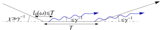
Figure 1: Diagram for collinear-collinear radiation interference from double hard scattered electron (high-$\omega$ spectral region).

An impetus to studies of nondipole radiation from high-energy electrons was given by recent experimental investigation of radiation at double scattering [5], aiming at verification of predictions [6, 7, 8] about interference fringes in spectra of bremsstrahlung on two amorphous foils. Such fringes may basically be described by classical electrodynamics (granted that typical photon energies $\hbar\omega$ are much lower than the electron energy). Embarking at the textbook formula for spectral distribution of irradiated energy

$$\frac{dI}{d\omega}=\omega^{2}\int d^{2}n\left|\frac{e}{2\pi}\int_{-\infty}^{\infty}dt[\vec{n},\vec{v}(t)]e^{i\omega t-i\vec{k}\cdot\vec{r}(t)}\right|^{2},$$ (1)

(we let $c=1$), one can bring it to a form of a single integral [9]

$$\left\langle\frac{dI}{d\omega}\right\rangle_{1,2}=\left\langle\frac{dI_{\text{BH}}}{d\omega}\right\rangle_{1}+\left\langle\frac{dI_{\text{BH}}}{d\omega}\right\rangle_{2}-\frac{2e^{2}\gamma^{4}}{\pi}\!\int_{0}^{\infty}\!d\theta^{2}\theta^{2}\left\langle G\right\rangle_{1}\!\left\langle G\right\rangle_{2}\cos\left[\frac{\omega T}{2\gamma^{2}}(1+\gamma^{2}\theta^{2})\right],$$ (2)

where $\gamma=1/\sqrt{1-v^{2}}$ is the electron Lorentz factor, $\theta$ the radiation emission angle with respect to the intermediate electron line,

$$G(\theta)\approx\frac{1}{1+\gamma^{2}\theta^{2}}-\frac{1}{2\gamma^{2}\theta^{2}}\left(1+\frac{\theta^{2}-\chi^{2}-\gamma^{-2}}{\sqrt{[\gamma^{-2}+(\theta-\chi)^{2}][\gamma^{-2}+(\theta+\chi)^{2}]}}\right),$$

and $\left\langle...\right\rangle$ denotes the averaging over electron scattering angles $\chi_{1}$ and $\chi_{2}$ in each foil. The last term in (2) gives rise to oscillatory spectral behavior

$$\left\langle\frac{dI}{d\omega}\right\rangle_{1,2}\underset{\omega\gg\gamma^{2}/T}{\simeq}\left\langle\frac{dI_{\text{BH}}}{d\omega}\right\rangle_{1}+\left\langle\frac{dI_{\text{BH}}}{d\omega}\right\rangle_{2}+\frac{8e^{2}}{\pi}\left\langle G(0)\right\rangle_{1}\left\langle G(0)\right\rangle_{2}\left(\frac{2\gamma^{2}}{\omega T}\right)^{2}\cos\frac{\omega T}{2\gamma^{2}},$$ (3)

$$\frac{dI_{\text{BH}}}{d\omega}(\gamma\chi)\underset{\gamma\chi\gg 1}{\simeq}\frac{2e^{2}}{\pi}(\ln\gamma^{2}\chi^{2}-1)$$ (4)

[with $G(0)=1-\frac{1}{\left(1+\gamma^{2}\chi^{2}\right)^{2}}$], which is similar to that for interference of transition radiation from different boundaries of the traversed plate [2], or to that for radiation in a gap of a storage ring [3]. The phase of the cosine in Eq. (3) may be understood as the physical ratio ${\omega T}/{2\gamma^{2}}=T/l_{0}(\omega)$, where

$$l_{0}(\omega)=\frac{2\gamma^{2}}{\omega}$$ (5)

is the “free” photon formation length. Notably, oscillations (3) enhance in the highly non-dipole regime $\gamma^{-1}\ll\chi\ll 1$, when $G\underset{\chi\gg\gamma^{-1}}{\to}\frac{1}{1+\gamma^{2}\theta^{2}}$, becoming independent of the scattering angles which are averaged over. That is not unnatural, as long as in the opposite, dipole limit their average must vanish (dipole Bethe-Heitler contributions do not interfere on the average).

One may ask, however, why does the phase of the interference term depend on $T/l_{0}(\omega)$ alone, but is independent of the electron scattering angles. It might as well depend on the scattering-modified photon formation length

$$l_{\chi}(\omega)\simeq l_{f}(\omega,\theta)\big{|}_{\theta\sim\chi}\equiv\frac{2}{\omega(\gamma^{-2}+\theta^{2})}\bigg{|}_{\theta\sim\chi}\sim\frac{2}{\omega\chi^{2}}\qquad\quad(\chi\gg\gamma^{-1})$$ (6)

relevant, e.g., in the theory of Landau-Pomeranchuk-Migdal effect [10], which, after all, is just another manifestation of radiation interference. A closer examination reveals that in the two-foil case, interference effects related with length (6) are erased by averaging. But for problems without averaging, they may be viable and observable.

Whereas from Fig. 1 it is clear which kinds of photons are interfering on scale $l_{0}(\omega)$, for scale $l_{\chi}(\omega)$ that may be less obvious. In what follows, we shall demonstrate that the interference at low $\omega$ involves nontrivial geometry both in the longitudinal and transverse directions, and engages not one but two categories of photons: intra-jet (inside a jet formed by a temporarily straight moving electron) and inter-jet (between the jets) [11]. Therefore, the mechanism of edge radiation interference at low $\omega$ is not the same as at high $\omega$, but more intricate.

At the same time, all highly-nondipole radiation problems in finite targets have much in common. In this paper, we propose a generalization for their spectral decomposition. It seems expedient to begin with its statement.

2 Separation of volume and edge contributions for nondipole radiation in finite targets

To assess edge effects, first of all, it is imperative to define how to discriminate them from the volume contribution. A natural and generally applicable procedure is to indefinitely expand the target (i.e., formally send its size $T\to\infty$ with the rest of the parameters held fixed), and split

$$\frac{dI}{d\omega}=\frac{dI_{\text{vol}}}{d\omega}+\frac{dI_{b}}{d\omega},$$ (7)

where $\frac{dI_{\text{vol}}}{d\omega}\propto T$ [i.e., $\frac{dI_{\text{vol}}}{d\omega}=T\left(\underset{T\to\infty}{\lim}\frac{1}{T}\frac{dI}{d\omega}\right)$], and $\frac{dI_{b}}{d\omega}\underset{T\to\infty}{=}O(1)$.

The leading, “volume” contribution $\frac{dI_{\text{vol}}}{d\omega}$ is expected to be generated “locally” (i.e., at spatial scales much smaller than $T$). So, it must depend on $\omega$ essentially through the ratio

$$\frac{l_{\text{ext}}}{l_{0}(\omega)}.$$ (8)

Here $l_{\text{ext}}=\max\tau(\chi\lesssim\gamma^{-1})$ is the time scale within which the electron deflection angles do not overwhelm typical radiation emission angles $\sim\gamma^{-1}$, and thereby the radiation coherence is maintained. Hence, $l_{\text{ext}}$ plays the role of the external field coherence length.

The remainder $\frac{dI_{b}}{d\omega}$, which must embody all the edge effects, should depend on variable (8) somewhat differently, because it is generated in a physically different way. Besides that, it can depend on a ratio

$$\frac{T}{l_{\chi}(\omega)}.$$ (9)

But when scales of $\omega$, at which variables (8) and (9) are of the order of unity, vastly differ ($\chi\gg\gamma^{-1}$), the dependence of $\frac{dI_{b}}{d\omega}$ on them may actually be treated as additive.

To gain more insight into the structure of edge effects, it should be realized that in the angular distribution of highly nondipole radiation on a finite target there are always prominent jets. They are related with formation of photons attached to the initial or the final electron line during long times, and thereby being narrowly collimated (to within angles $\sim\gamma^{-1}$ around the electron velocity). Besides that, radiation persists also at angles between the jets, being fainter but filling a wider angular region (see, e.g., Fig. 2 of [11]). Even though in radiation spectra the emission angles are integrated over, jet effects can survive under conditions of nondipole radiation. In a generic case considered herein, these jets do not overlap in the plane of emission angles, and thus do not interfere, but jet photons from one electron line can interfere with interjet photons emitted at the opposite boundary of the target.

Under the given conditions, the formal additivity of manifestations of the two scales in the radiation spectrum has a clear-cut physical meaning. In decomposition

$$\frac{dI_{b}}{d\omega}\underset{\chi\gg\gamma^{-1}}{\simeq}2\frac{dI_{1b}}{d\omega}\left(\frac{l_{\text{ext}}}{l_{0}(\omega)}\right)+\frac{dI_{bb}}{d\omega}\left(\frac{T}{l_{\chi}(\omega)}\right),\qquad\frac{dI_{bb}}{d\omega}\underset{T/l_{\chi}\to 0}{\to}0,$$ (10)

$\frac{dI_{1b}}{d\omega}$ corresponds to a single-boundary contribution, and is normally independent of $T$, as well as of the wide deflection angles collectively denoted here as $\chi$. On the other hand, $\frac{dI_{bb}}{d\omega}$ corresponds to effects of interference between the boundaries, and appears to be basically independent of $\gamma$. More precisely, since $\frac{dI_{bb}}{d\omega}$ generally involves some jet effects, too, sp it bears a mild $\gamma$-dependence, generally being expressible as

$$\frac{dI_{bb}}{d\omega}=\frac{2e^{2}}{\pi}\left[2A_{1}\left(\frac{\omega T\chi^{2}}{2}\right)F_{\perp}\left(\frac{\omega T\chi}{\gamma}\right)+A_{2}\left(\frac{\omega T\chi^{2}}{2}\right)\right].$$ (11)

Functions $A_{1}$ and $A_{2}$ usually are oscillatory and decreasing as power laws. They may be called “quasi-antenna” formfactors, where the role of the “antenna” is played by the sufficiently bent electron’s trajectory (abstracting from the electron as a pointlike particle), which may be treated as a long “wire”, along which the electric current evoked by the electron motion flows essentially at the speed of light ($\gamma\to\infty$). In turn, $F_{\perp}$ is a monotonously decreasing proper field formfactor, absorbing all the jet effects, and furnishing exponential decrease of the oscillations at intermediate $\omega$.

In separation (10), single and double boundary contributions are logarithmically divergent individually (cf., e.g., [13]),

$$2\frac{dI_{1b}}{d\omega},\frac{dI_{bb}}{d\omega}\underset{\omega\to 0}{\sim}\pm\ln\frac{1}{\omega},$$ (12)

but the divergences cancel in their sum.

The quoted formulas pertain to the case when the target edges are sharp. To take their non-zero width $\Delta T\ll T$ into account, one has to replace

$$\frac{dI_{1b}}{d\omega}\to\frac{dI_{1b}}{d\omega}F_{\text{edge}}(\omega\Delta T/\gamma^{2}),$$ (13)

with an additional formfactor $F_{\text{edge}}$, whereas contributions $\frac{dI_{\text{vol}}}{d\omega}$, $\frac{dI_{bb}}{d\omega}$ are unaltered.

3 Non-dipole spectral decompositions for specific problems

3.1 Radiation in a finite magnet

To illustrate the conjectured decomposition, consider a few specific examples. First, consider a process of radiation from a fast electron passing through a long but finite magnet (see Fig. 2). This physical problem was studied on general grounds in [4], but our objective is to decouple single-edge and edge interference contributions based on the long-magnet asymptotics.

In this case, for all $\omega$ it is advantageous to employ for the radiation spectrum the double time integral representation [see [15] and Eq. (31) below]. The result of the integrations gives structure (7), (10) with entries

$$\frac{dI_{\text{vol}}}{d\omega}=2e^{2}X\left\{-(2\Omega_{s})^{1/3}\text{Ai}^{\prime}\left[(2\Omega_{s})^{2/3}\right]-\Omega_{s}\int_{(2\Omega_{s})^{2/3}}^{\infty}d\alpha\text{Ai}(\alpha)\right\}$$ (14)

(representing the synchrotron radiation intensity times the magnet length, $\Omega_{s}=\frac{\omega R}{2\gamma^{3}}$, $X=\frac{\gamma T}{R}=\gamma\chi$, $R$ stands for the trajectory bending radius),

$$\frac{\pi}{e^{2}}\frac{dI_{1b}}{d\omega}=(2\Omega_{s})^{\frac{2}{3}}\pi\text{Gi}\left[(2\Omega_{s})^{\frac{2}{3}}\right]-3\qquad\qquad\qquad\qquad\qquad\qquad\qquad\qquad\qquad\qquad$$

$$+\int_{1}^{\infty}\!\!\!\frac{dw}{w-\frac{3}{4}}\Bigg{\{}1+\Omega_{s}^{\frac{2}{3}}\!\left[2\!\left(\!1-\frac{3}{4w}\right)^{\!\frac{2}{3}}\!\!-w\left(\!1-\frac{3}{4w}\right)^{\!-\frac{1}{3}}\right]\!\pi\text{Gi}\!\left(\Omega_{s}^{\frac{2}{3}}w\!\left(\!1-\frac{3}{4w}\right)^{\!-\frac{1}{3}}\right)\!\!\Bigg{\}},$$

(15)

where $\text{Gi}(\alpha)=\frac{1}{\pi}\int_{0}^{\infty}dt\sin\left(\alpha t+\frac{1}{3}t^{3}\right)$ is the Scorer function, arising naturally instead of the Airy function $\text{Ai}(\alpha)=\frac{1}{\pi}\int_{0}^{\infty}dt\cos\left(\alpha t+\frac{1}{3}t^{3}\right)$ in description of single-edge effects, and finally,

$$\frac{dI_{bb}}{d\omega}=\frac{2e^{2}}{\pi}\left[2A_{1}\left(\Omega_{s}X^{3}\right)F_{\perp}(\Omega_{s}X^{2})+A_{2}\left(\Omega_{s}X^{3}\right)\right],$$ (16)

where

$$F_{\perp}(z)=zK_{1}(z),\qquad F_{\perp}(0)=1$$ (17)

is a proper field form factor [11], whose relevance for the present process will be elucidated in Sec 4.1, whereas antenna formfactors are

$$A_{1}=\frac{2}{\Omega_{s}X^{3}}\int_{0}^{\infty}\frac{du}{(1+u)^{2}}\Bigg{\{}\sin\left[\frac{\Omega_{s}X^{3}}{3}(1+u)\right]-\sin\left[\frac{\Omega_{s}X^{3}}{2}\left(\frac{2}{3}+u\right)\right]\Bigg{\}},$$ (18)

$$A_{2}=\int_{0}^{\infty}\frac{du}{1+u}\Bigg{\{}\cos\left[\frac{\Omega_{s}X^{3}}{12}(1+3u)\right]-\cos\left[\frac{\Omega_{s}X^{3}}{12}(1+u)\right]$$

$$+\frac{2}{1+u}\cos\left[\frac{\Omega_{s}X^{3}}{12}(1+u)^{3}\right]\Bigg{\}}.$$ (19)

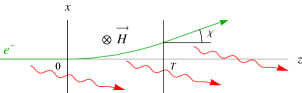
Figure 2: Geometry of radiation from an electron in a finite magnet. Photon emissions from the three distinct spatial regions are generally interfering.

In spite of some bulkiness of the encountered formulae, the present case is the most “normal” manifestation of decomposition (7), (10): Structure (16) exactly corresponds to conjectured representation (11), while (3.1) depends solely on $\Omega_{s}$, which may be cast in form (8), (5) with $l_{\text{ext}}=R/\gamma$.

Single-boundary contribution $\frac{dI_{1b}}{d\omega}$ (an analog of transition radiation, arising in the absence of atomic matter) is not positive definite, so, it does not give an independent radiation intensity, and needs a sufficient volume radiation background. Its salient feature is that at high $\omega$, the edge contribution falls off as a (positive) power law

$$\frac{dI}{d\omega}\underset{\Omega_{s}\to\infty}{\simeq}2\frac{dI_{1b}}{d\omega}\simeq\frac{7e^{2}}{15\pi\Omega_{s}^{2}},$$ (20)

which must ultimately dominate over the exponentially attenuating volume synchrotron contribution. Qualitative prediction of asymptotic behavior $\frac{dI}{d\omega}\underset{\omega\to\infty}{\sim}\omega^{-2}$ was made in [4].

At low $\omega$, terms (3.1) and (18) combine to mutually cancel their logarithmic singularities [cf. Eq. (12)] and ensure the correspondence with the factorization theorem.

A related problem arises for radiation at electron passage through a short crystal (see, e.g., [14]), particularly when the electron passing through the inter-planar channel nearly conserves its impact parameter, thus experiencing a constant transverse force. In that case, the target edges are sharper than those for laboratory magnets, but there arises an additional need for averaging over electron impact parameters.

3.2 Bremsstrahlung at double hard scattering

A subtler example, already mentioned in the Introduction, arises when instead of interaction with a continuous target, the electron undergoes two instantaneous scatterings. Specifically, let the electron scatter repeatedly, at points separated by a time interval $T$, through angles $\vec{\chi}_{1}$, $\vec{\chi}_{2}$ with a relative azimuth $\varphi_{12}=\arccos\left(\vec{\chi}_{1}\cdot\vec{\chi}_{2}/|\vec{\chi}_{1}||\vec{\chi}_{2}|\right)$, such that $|\vec{\chi}_{1}|,|\vec{\chi}_{2}|\gg\gamma^{-1}$. After appropriate integrations in (1), one arrives [11] at the expression for the radiation spectrum (7), (10), with

$$\frac{dI_{\text{vol}}}{d\omega}=\sum_{i=1}^{2}\frac{dI_{\text{BH}}}{d\omega}(\gamma\chi_{i}),$$ (21)

$$\frac{dI_{1b}}{d\omega}=-\frac{e^{2}}{\pi}\int_{0}^{\infty}\frac{d\theta^{2}\theta^{2}}{(\gamma^{-2}+\theta^{2})^{2}}\cos\left[\frac{\omega T}{2\gamma^{2}}\left(1+\gamma^{2}\theta^{2}\right)\right]$$ (22)

[the latter being similar to the non-dipole limit of the non-averaged interference term in (2)], and

$$\frac{dI_{bb}}{d\omega}=\frac{2e^{2}}{\pi}\Bigg{[}A_{1}\left(\frac{\omega T\chi_{1}^{2}}{2},\frac{\omega T\chi_{1}{\chi}_{2}}{2}e^{i\varphi_{12}}\right)F_{\perp}\left(\frac{\omega T\chi_{1}}{\gamma}\right)\qquad\qquad\qquad\qquad$$

$$+A_{1}\left(\frac{\omega T\chi_{2}^{2}}{2},\frac{\omega T\chi_{1}{\chi}_{2}}{2}e^{i\varphi_{12}}\right)F_{\perp}\left(\frac{\omega T\chi_{2}}{\gamma}\right)+A_{2}\left(\frac{\omega T\chi_{1}{\chi}_{2}}{2}e^{i\varphi_{12}}\right)\Bigg{]}\quad$$ (23)

with

$$A_{1}\left(z_{1},z_{2}\right)=-\text{Ci}\left(z_{1}\right)+\mathfrak{Re}\left\{\cos z_{2}\text{Ci}\left(z_{1}+z_{2}\right)+\sin z_{2}\text{si}\left(z_{1}+z_{2}\right)\right\},$$ (24)

$$A_{2}\left(z\right)=-\mathfrak{Re}\left\{\cos z\text{Ci}\left(z\right)+\sin z\text{si}\left(z\right)\right\},$$ (25)

$\text{Ci}(z)=-\int_{z}^{\infty}\frac{dx}{x}\cos x$, $\text{si}(z)=-\int_{z}^{\infty}\frac{dx}{x}\sin x$, and $F_{\perp}$ given by Eq. (17). Contributions (22) and (24), (25), depending on different photon formation lengths, exhibit oscillations in different spectral regions (see Fig. 3). Presently, only hard oscillations (22), corresponding to formation length $l_{0}$ were investigated experimentally [5].

Figure 3: (Adapted from Ref. [11].) Spectrum of electromagnetic radiation from an electron scattering two times through co-planar ($\varphi_{12}=0$) equal angles $\chi=30\gamma^{-1}$. Dot-dashed curve, Eq. (32).

Comparison of the obtained structures with generic Eqs. (10), (11) indicates that (3.2) is perfectly consistent with (11). However, since now $l_{\text{ext}}=\max\tau(\chi\lesssim\gamma^{-1})=T$ (in spite that angles $\sim\chi$ are also achieved at scattering in single points), (22) depends on $T$, and therefore it is not quite a single-boundary contribution. Still, it can be treated as such, in the sense that the photons are formed only on one of the boundaries, but contributions from different boundaries can interfere. But a $T$-dependent scale can already not be relevant for $\frac{dI_{\text{BH}}}{d\omega}$. Fortunately, since the latter is actually $\omega$-independent [see Eq. (4)], the problem does not exist. Physically, the encountered anomaly owes to the straightness of the electron motion in between the scattering points, so that even if photons are formed at its ends pretty far from each other, they move in the same direction and hence can interfere, as was depicted in Fig. 1.

A more serious issue arises when initial and final electrons are collinear [see Fig. 5(c) of [11]]. Such effects are not taken into account by the decomposition of Sec. 2. In particular, they should include also an overlap of two formfactors $F_{\perp}$, corresponding to initial and final electron states. But the latter case may be regarded as exceptional.

4 Space-time analysis

Proper understanding of the structure of the encountered spectral decomposition (11) requires studying its space-time origin. Below we will explain in a nutshell the physical mechanisms behind this structure.

4.1 Intermediate $\omega$. Ray optics

As was already mentioned in the Introduction, at high $\omega$ the interference is governed by the longitudinal coherence with length $l_{0}$. With the decrease of $\omega$, transverse wavelengths increase and become comparable with the geometrical transverse scales. So, there increases the importance of proper treatment of transverse spatial dimensions. They can be brought out, e.g., by passing, via Fourier transformation, from radiation emission angles to photon impact (or emission) parameters. For single scattering, such a photon impact parameter representation is rather well-known [18, 7, 19]:

$$\frac{dI}{d\omega}=\left(\frac{e}{\pi}\right)^{2}\int d^{2}\xi\left[\frac{\partial}{\partial\vec{\xi}}K_{0}(\xi/\gamma)\right]^{2}\left|1-e^{i\vec{\chi}\cdot\vec{\xi}}\right|^{2}=\frac{dI_{\text{BH}}}{d\omega}(\gamma\chi),$$ (26)

where $\vec{b}=\vec{\xi}/\omega$ is the impact parameter. Integration in (26) recovers form (4).

An extension of this approach to double scattering leads to representation [9, 11]

$$\frac{dI}{d\omega}=\frac{dI_{\text{BH}}}{d\omega}(\gamma\chi_{1})+\frac{dI_{\text{BH}}}{d\omega}(\gamma\chi_{2})\qquad\qquad\qquad\qquad\qquad\qquad$$

$$-\frac{e^{2}}{\pi^{3}\omega T}\iint d^{2}\xi_{1}d^{2}\xi_{2}\frac{\partial}{\partial\vec{\xi}_{1}}K_{0}\left(\frac{\xi_{1}}{\gamma}\right)\cdot\frac{\partial}{\partial\vec{\xi}_{2}}K_{0}\left(\frac{\xi_{2}}{\gamma}\right)\qquad$$

$$\times\mathfrak{Im}\left\{\left(1-e^{-i\vec{\chi}_{1}\cdot\vec{\xi}_{1}}\right)\left(1-e^{-i\vec{\chi}_{2}\cdot\vec{\xi}_{2}}\right)e^{-i\frac{\omega T}{2\gamma^{2}}+i\frac{(\vec{\xi}_{1}-\vec{\xi}_{2})^{2}}{2\omega T}}\right\}.$$ (27)

On its basis, it is straightforward to demonstrate the onset of ray optics in the given process: When $\chi\gg\gamma^{-1}$, exponentials $e^{-i\vec{\chi}_{1}\cdot\vec{\xi}_{1}}$, $e^{-i\vec{\chi}_{2}\cdot\vec{\xi}_{2}}$ are rapidly oscillating, and along with the Gaussian factor $e^{i\frac{(\vec{\xi}_{1}-\vec{\xi}_{2})^{2}}{2\omega T}}$, they form (real) stationary phase points, defining rays parallel to one of the external electron lines. The monotonous decrease of the impact-parameter-dependent photon distributions at these impact parameters gives rise to the proper field formfactor for $A_{1}$ – see Fig. 4(a). On the contrary, Fig. 4(b) demonstrates the absence of a modulating formfactor for $A_{2}$.

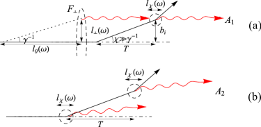
Figure 4: (a) Graphical illustration of formation of the jet-interjet interference contribution $A_{1}$ and its modulating formfactor $F_{\perp}$. The condition of interference between collinear and noncollinear photons, besides the coincidence of emission directions, is the equality of impact parameters: $l_{\perp}(\omega)={\gamma}/{\omega}$ and $b_{i}\sim T\chi$. There is also a cross diagram, in which interjet photons are emitted from the first scattering vertex, and jet ones from the final electron line. (b) The same for interjet-interjet interference contribution $A_{2}$.

In the case of radiation in a magnet, it should be remembered yet that synchrotron photons within the magnet are stripped at a non-zero intrinsic impact parameter

$$\Delta x_{\text{syn}}=\xi_{x}/\omega\sim R^{1/3}\omega^{-2/3}.$$ (28)

At small $\omega$, that quantity is large, but with the increase of $\omega$, it ultimately falls below the impact parameter difference between electron entrance and exit from the magnet:

$$b_{i}=\left|\int_{0}^{T}dt\left[\vec{\chi}(t)-\vec{\chi}_{i}\right]\right|=T^{2}/2R,$$ (29)

or

$$b_{f}=\left|\int_{0}^{T}dt\left[\vec{\chi}_{f}-\vec{\chi}(t)\right]\right|=T^{2}/2R,$$ (30)

which are independent of $\omega$. That happens at $\Delta x_{\text{syn}}\ll b_{i},b_{f}$, i.e., $\omega T\chi^{2}\gg 1$, which is exactly the region where oscillations of $A_{1}$ develop. Then, $b_{i},b_{f}$ become sufficiently sharply defined, so the electron proper field amplitude (17) factors out with $b\to b_{i},b_{f}$, and its exponential falloff at large $\omega$ eventually suppresses the spectral oscillations.

4.2 Low $\omega$. “Radio” contribution

At sufficiently low $\omega$, the ray optics concepts break down, isolated points no longer play a distinguished role, and the entire electron trajectory radiates as a whole. At that, the foreground is taken by time aspects.

Formally, at $\omega\to 0$, there emerges a hierarchy of time scales, some of which, being reciprocal to $\omega$, expand indefinitely, whereas others, determined by the target thickness, remain finite. To carry out the corresponding scale separation self-consistently, it is convenient to embark at the representation for radiation spectrum, in which integration over photon emission angles is performed exactly. The resulting double time integral representation expresses covariantly as [11]

$$\frac{1}{\omega}\frac{dI}{d\omega}=\frac{e^{2}}{\pi}\mathfrak{Im}\int_{-\infty}^{\infty}ds_{2}\int^{s_{2}}_{-\infty}ds_{1}u_{\mu}(t_{1})u_{\nu}(t_{2})e^{-i\omega(t_{2}-t_{1})}D_{\mu\nu}\left(\omega,\left|\vec{r}(t_{2})-\vec{r}(t_{1})\right|\right)$$ (31)

and may be viewed as a kind of unitarity relation (see Fig. 5). Here $s=t/\gamma$ is the electron proper time, $u_{\mu}$ its 4-velocity, and $D_{\mu\nu}$ the photon propagator. Specializing $D_{\mu\nu}$ in the frequency-position representation and Feynman gauge, $D_{\mu\nu}(\omega,r)=-\frac{g_{\mu\nu}}{r-i0}e^{i\omega r}$, reproduces the widely used formula [15], whereas isolating the imaginary part of $\frac{1}{r-i0}$ and presenting it in an integral form through a “vacuum” term, to representation [16].

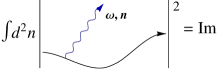
Figure 5: Graphical illustration of unitarity relation (31).

With the aid of formula (31), one can derive a next-to-leading order (NLO) correction to the low-$\omega$ approximation:

$$\frac{dI}{d\omega}\underset{\omega\to 0}{\simeq}\frac{dI_{\text{BH}}}{d\omega}(\gamma\chi)+C_{1}\omega+\mathcal{O}(\omega^{2}),$$ (32)

where the first (LO) term is the well-known factorization limit given by Eq. (4), and the coefficient at the NLO term reads [17]

$$C_{1}=-\frac{e^{2}}{2}\int_{-\infty}^{\infty}dt[\vec{\chi}(t)-\vec{\chi}_{i}]\cdot[\vec{\chi}_{f}-\vec{\chi}(t)],$$ (33)

with $\vec{\chi}_{i}$ and $\vec{\chi}_{f}$ being the initial and final electron deflection angles. The physical meaning of $C_{1}$ is that apart from the $e^{2}$ factor, it represents the difference between the time delay for the actual trajectory and for its angle-shaped approximation [17].

From Eq. (33), it is evident that for monotonous electron deflection (in particular, for cases considered in Secs. 3.1, 3.2), always $C_{1}<0$. Therefore, in those cases the spectrum suppression at low $\omega$ is non-monotonous.

The salient feature of $C_{1}$ is its independence of $\gamma$ (or electron mass) for a definite trajectory $\vec{\chi}(t)$, i.e., definite particle energy and the field strength. Continuing the analysis under this assumption to all higher orders in $\omega$, one would recover complete antenna formfactors (11), which are functions of a $\gamma$- (or mass-) independent product $\omega T\chi^{2}$.

5 Bremsstrahlung in an amorphous plate

Yet another, and perhaps practically most important example of a target with sharp boundaries is a solid plate (in the simplest case – amorphous). The volume contribution in this case is described by

$$\frac{dI_{\text{vol}}}{d\omega}=\left\langle\frac{dI_{\text{BH}}}{d\omega}\right\rangle\Phi_{M}(s),$$ (34)

with $\left\langle\frac{dI_{\text{BH}}}{d\omega}\right\rangle=\frac{2e^{2}}{3\pi}\gamma^{2}\left\langle\chi^{2}\right\rangle$ and the Migdal function [21]

$$\Phi_{M}(s)=6s^{2}\left\{4\mathfrak{Im}\psi\left[(1+i)s\right]-\frac{1}{s}-\pi\right\},\qquad\Phi_{M}(s)\underset{s\to\infty}{\to}1,$$ (35)

involving $\psi(z)=\Gamma^{\prime}(z)/\Gamma(z)$ and the argument related to ratio (8) by

$$8s^{2}=\frac{l_{\text{ext}}}{l_{0}(\omega)}=\frac{\omega}{2\gamma^{4}d\left\langle\chi^{2}\right\rangle/d\tau}.$$ (36)

The single-boundary contribution, evaluated in [13], may be expressed as

$$\frac{dI_{1b}}{d\omega}=\frac{e^{2}}{\pi}B(2(1+i)s),$$ (37)

$$B(\sigma) = \mathfrak{Re}\Bigg{\{}2\sigma\int_{0}^{\infty}dxE_{1}\left[\sigma\tanh x\right]e^{-\sigma(x-\tanh x)}-2$$ (38)

$$+\int_{0}^{\infty}dxe^{-\sigma x}\left(1-\sigma x\right)\left(\coth x-\frac{1}{x}\right)\Bigg{\}},\qquad B(\sigma)\underset{s\to\infty}{\to}0,$$

and $E_{1}(z)=\int_{z}^{\infty}\frac{dx}{x}e^{-x}$. It features a logarithmic infrared divergence. Boundary-boundary interference contribution can be read off from Eq. (6.13) of [19]:

$$\frac{dI_{bb}}{d\omega}=\frac{2e^{2}}{\pi}A\left(\frac{\omega T\left\langle\chi^{2}\right\rangle}{2}\right),$$ (39)

$$A(z)=\ln\left(2|\sinh\sqrt{iz}|\right)-\sqrt{z/2},$$ (40)

where the last term is the subtraction corresponding to the infrared square root singularity contained in (34), (35), and also ensuring that $A(z)\underset{z\to\infty}{\to}0$.

Figure 6: Normalized spectrum of bremsstrahlung on an amorphous plate, in which the final rms deflection angle equals $\sqrt{\left\langle\chi^{2}\right\rangle}=5\gamma^{-1}$. Dashed curve is the pure volume contribution (34), (35). Dot-dashed, volume two plus single-boundary contributions (37), (38). Solid curve is the sum of all contributions.

In contrast to (18)–(3.1) and (24)–(25), contribution (40) due to the interference between the boundaries is not oscillatory. That is natural, as long as those oscillations depend on the final electron deflection angle, but in the present problem it is random, and is averaged over, thereby erasing the oscillations. Therewith also disappears the need for the attenuation formfactor $F_{\perp}$, which may be put equal to unity.

The behavior of a typical highly-nondipole radiation spectrum evaluated by Eqs. (34)–(40), along with its partial contributions, is shown in Fig. 6. At $\omega\to 0$, it tends to the value dictated by the infrared factorization theorem (see [9] and refs. therein). In practice, at $\omega\to 0$ there may also arise a bump due to transition radiation, which was not taken into account within the present treatment [22].

6 Summary and outlook

In spite of the diversity of possible electron scattering configurations in finite targets, the corresponding radiation spectra admit similar decompositions, as described in Sec. 2. Understanding of the underlying radiation mechanisms helps to determine which coherence length is relevant for which photon frequency range.

There are certain exceptions from the simplest variant of the decomposition theorem described here. Some of them were mentioned in Secs. 3.2 and 5. They merit more detailed investigation in the future.

The relationship between the novel interference features discussed in the present article and jet and interjet, as well as time delay concepts of high-energy electrodynamics, permitting the neglect of the charged particle mass, opens new vistas for their investigation, with possible extensions to nuclear and hadron physics (cf., e.g., [23, 24]). The parallelism with radio- and antenna physics may bring new tools for the theory development. Investigations of radiation spectra behavior at low $\omega$ is also important from the applied point of view.

References

• [1] V.L. Ginzburg, Theoretical Physics and Astrophysics (Oxford: Pergamon Press, 1979).
• [2] P. Rullhusen, X. Artru, P. Dhez, Novel Radiation Sources using Relativistic Electrons (Singapore: World Scientific, 1998).
• [3] O.V.Β Chubar and N.V.Β Smolyakov, J. Optics (Paris) 24, 117 (1993); R.A.Β Bosch, Il Nuovo Cim. 20, 483 (1998).
• [4] V.G.Β Bagrov, N.I. Fedosov, and I.M.Β Ternov, Zh. Eksp. Teor. Fiz. 82, 1442 (1982) [Sov. Phys. JETP 55, 835 (1982)]; Phys. Rev. D 28, 2464 (1983).
• [5] K.K.Β Andersen et al., Phys. Lett. B 732, 309 (2014).
• [6] R.Β Blankenbecler, Phys. Rev. D 55, 190 (1997).
• [7] B.G. Zakharov, Pis’ma Zh. Eksp. Teor. Fiz. 64, 737 (1996) [JETP Lett. 64, 781 (1996)]; Yad. Fiz. 61, 924 (1998) [Phys. At. Nucl. 62, 1008 (1998)].
• [8] V.N. Baier and V.M. Katkov, Phys. Rev. D 60, 076001 (1999).
• [9] M.V.Β Bondarenco and N.F.Β Shul’ga, Phys. Rev. D 90, 116007 (2014).
• [10] V.M.Β Galitsky and I.I.Β Gurevich, Nuov. Cim. 32, 396 (1964).
• [11] M.V.Β Bondarenco and N.F.Β Shul’ga, Phys. Rev. D 95, 056003 (2017).
• [12] C. Carimalo, A. Schiller, and V.G. Serbo, Eur. Phys. J. C 23, 633 (2002).
• [13] I.I. Gol’dman Zh.E.T.F. 38, 1866 (1960) [Sov. Phys. JETP 11, 1341 (1960)].
• [14] Y. Takabayashi, V.G. Bagrov, O.V. Bogdanov, Yu.L. Pivovarov, and T.A.Β Tukhfatullin, NIM B 355, 188 (2015).
• [15] V.N.Β Baier, V.M.Β Katkov, V.M.Β Strakhovenko, Electromagnetic Processes at High Energies in Oriented Crystals (Singapore: World Scientific, 1998).
• [16] R.Β Blankenbecler and S.D.Β Drell, Phys. Rev. D 53, 6265 (1996).
• [17] M.V. Bondarenco, Phys. Rev. D 96, 076009 (2017).
• [18] J.D. Bjorken, J.B. Kogut, and D.E. Soper, Phys. Rev. D 3, 1382 (1971).
• [19] V.N. Baier and V.M. Katkov, Phys. Rev. D 57, 3146 (1998).
• [20] X. Artru, in: H. Wiedemann (Ed.), Advanced Radiation Sources and Applications, NATO Science Series II, 199, 387 (2006).
• [21] A. B.Β Migdal, Phys. Rev. 103, 1811 (1956).
• [22] S.Β Klein, Rev. Mod. Phys. 71, 1501 (1999).
• [23] R.M. Eisberg, D.R. Yennie, and D.H. Wilkinson, Nucl. Phys. 18, 338 (1960).
• [24] Yu.L.Β Dokshitzer, V.A.Β Khoze, A.H.Β Mueller, S.I.Β Troyan. Basics of Perturbative QCD, Paris: Editions Fontieres, 1991.