Determining the Absolute Magnitudes of Galactic-Bulge Red Clump Giants in the Z and Y Filters of the Vista Sky Surveys and the IRAC Filters of the Spitzer Sky Surveys

Аннотация

The properties of red clump giants in the central regions of the Galactic bulge are investigated in the photometric $Z$ and $Y$ bands of the infrared VVV (VISTA/ESO) survey and the [3.6], [4.5], [5.8], and [8.0] bands of the GLIMPSE (Spitzer/IRAC) Galactic plane survey. The absolute magnitudes for objects of this class have been determined in these bands for the first time: $M_{Z}=-0.20\pm 0.04$ and $M_{Y}=-0.470\pm 0.045$, $M_{[3.6]}=-1.70\pm 0.03$, $M_{[4.5]}=-1.60\pm 0.03$, $M_{[5.8]}=-1.67\pm 0.03$ and $M_{[8.0]}=-1.70\pm 0.03$. A comparison of the measured magnitudes with the predictions of theoretical models for the spectra of the objects under study has demonstrated good mutual agreement and has allowed some important constraints to be obtained for the properties of bulge red clump giants. In particular, a comparison with evolutionary tracks has shown that we are dealing predominantly with the high- metallicity subgroup of bulge red clump giants. Their metallicity is slightly higher than has been thought previously, $[M/H]\simeq 0.40$ ($Z\simeq 0.038$) with an error of $[M/H]\simeq 0.1$ dex, while the effective temperature is $4250\pm 150$ K. Stars with an age of 9-10 Gyr are shown to dominate among the red clump giants, although some number of younger objects with an age of $\sim 8$ can also be present. In addition, the distances to several Galactic bulge regions have been measured, as D = 8200-8500 pc, and the extinction law in these directions is shown to differ noticeably from the standard one.

2018444248[264]

25 April 2017

1 INTRODUCTION

At present, the most commonly used filters in infrared astronomy are $J,H$ and $Ks$. Owing to the success of the 2MASS all-sky survey, they are the "golden standard"for the near-infrared photometry. Properties of objects of various classes, including red clump giants (RCGs), have been studied extensively in these filters (see, e.g., Paczynski and Stanek 1998; Girardi 1999, 2016). In particular, the absolute Ks magnitude for bulge RCGs $M_{Ks}=-1.61\pm 0.03$ (Alves 2000) and the corresponding intrinsic color $(J-Ks)_{0}=0.68\pm 0.03$ (Gonzalez et al. 2012) are adopted as the reference values. Despite the fact that the RCG population have a more complex and inhomogeneous structure than has been assumed previously (Gontcharov 2008; Bensby et al. 2013; Gontcharov and Bajkova 2013; Gonzalez et al. 2015), using the red clump centroid as a major tool for working with RCGs remains typical.

New sky surveys, in particular, VISTA (VVV and VHS) and UKIRT, have appeared in recent years. Apart from the photometry in the above three filters, measurements in several new ones, in particular, in the $Z$ and $Y$ filters that are already very close to the optical band, have also been performed. Mid-infrared Galactic surveys, for example, GLIMPSE onboard the Spitzer observatory in the [3.6], [4.5], [5.8], and [8.0] filters, are also of great importance. Using these data extends possibilities for investigating RCGs. In particular, photometric estimates made in a large number of filters can improve our understanding of the properties of these objects and can help in estimating the metallicity variations in the Galactic bulge. Furthermore, using RCGs, one can study the interstellar medium, in particular, determine the extinction value and law. Using additional filters leads to a more accurate and correct understanding of its properties.

However, before turning to the solution of particular problems, it is necessary to determine the reference points, namely the absolute magnitudes of RCGs in the corresponding filters. This is primarily true for the filters in which these magnitudes are not yet known – the $Z$ and $Y$ filters of the infrared VVV (VISTA/ESO) survey and the [3.6], [4.5], [5.8], and [8.0] bands of the GLIMPSE (Spitzer/IRAC) survey.

In this paper we consider several indirect methods to determine the absolute magnitudes of RCGs localized in the Galactic bulge. Before turning to their description and the results, several words should be said about the direct method. This method is the most obvious way of obtaining the absolute magnitudes and is based on a comparison of the catalogues from the surveys under study with the catalogue of stars with known parallaxes. In particular, this approach was applied by Laney et al. (2012) to determine the absolute magnitudes of nearby RCGs from 2MASS and Hipparcos data. This is also justified, because the absolute magnitudes of RCGs in the bulge and the solar neighborhood for the infrared agree satisfactorily between themselves.

The VISTA surveys and GAIA parallax measurements are a natural combination to determine the absolute $Z$ and $Y$ magnitudes of RCGs. However, this approach does not work at the current stage. One of the reasons is as follows: RCGs in the absence of a significant interstellar extinction are too bright even at fairly large distances, and their magnitudes in the VISTA surveys are among the overexposed ones. For example, the observed $Ks$ magnitude of RCGs is $\approx 8.3$, $\approx 10$, and $\approx 11$ at distances of 1, 2, and 3 kpc, respectively. At the same time, according to the data description, stars with magnitudes $m_{Ks}\simeq 10-12$ are overexposed in the VVV/VISTA survey.

In contrast, using more distant stars is so far impossible due to the insufficient accuracy of the parallaxes measured for them by the GAIA observatory and the presence of several significant systematic effects (Astraatmadja and Bailer-Jones 2016; Gontcharov 2017). Furthermore, at large distances the influence of interstellar extinction is already difficult to neglect. Under such conditions, the indirect methods of estimating the absolute magnitudes play an important role.

2 INSTRUMENTS AND DATA

In this paper we used the publicly available photo- metric data from VVV/ESO Data Release 4. For our study we selected the photometric magnitudes measured in the third standard $2\arcsec$. aperture. To perform our study in the mid-infrared, we used the combined mid-infrared data from the GLIMPSE surveys of the Spitzer Space Telescope obtained with the IRAC instrument. Detailed characteristics of the surveys and the filters can be found at these links, and they are briefly described in the final table containing our results.

To compare our results with theoretical stellar evolution models, we used the isochrones from the PARSEC database (Bressan et al. 2012; Marigo et al. 2017). We also used the SYNPHOT package for synthetic photometry and the Kurucz atlas of stellar atmospheres.

3 DETERMINING THE ABSOLUTE MAGNITUDES OF RCGs IN THE Z AND Y FILTERS

3.1 The First Method

Since direct estimations of the absolute magnitudes for nearby RCGs are fraught with a number of objective difficulties (see above), below we will investigate the properties of RCGs localized directly in the Galactic bulge, in the vicinity of Baade’s window. This and next sections will be devoted to describing the methods and elaborating the most optimal approach using, as an example, the determination of the absolute $Z$ and $Y$ magnitudes as the least-studied ones.

First of all, note that bulge RCGs have been comprehensively studied previously, and the general approaches are well known (see, e.g., Paczynski and Stanek 1998; Dutra et al. 2003; Revnivtsev et al. 2010; Gontcharov and Bajkova 2013). This section is based on the method proposed by Karasev et al. (2015) to determine the local extinction by in- vestigating the distribution of RCGs in narrow strips perpendicular to the Galactic plane. The strip width is $2\arcmin$, which allows the scatter of distances to RCGs due to the variability of the bulge structure along the Galactic longitude to be minimized (Nishiyama et al. 2009; Gonzalez et al. 2012). The vertical strip size spans the range of Galactic latitudes from $-5^{\circ}$ to $+5^{\circ}$ . Such a significant strip "height"is admissible, because it has been shown in several studies (see, e.g., Gerhard and Martinez-Valpuesta 2012) that the distance to the bulge changes little along the Galactic latitude. Thus, within such a strip it will everywhere be approximately the same. In addition, Gonzalez et al. (2015) concluded that the metallicity also depends weakly on the Galactic latitude (for $|b|<5^{\circ}$), i.e., within such a strip it must remain constant. It should also be noted that in the subsequent analysis, as in Revnivtsev et al. (2010) and Karasev et al. (2010a), all of the absorbing material is assumed to be in front of the bulge.

Figures 1 and 2 show examples of the color – apparent magnitude diagrams for all stars of such a strip in different sets of filters. The branch formed by RCGs from different parts of the strip (i.e., located at different latitudes) is clearly seen on each diagram. Such RCGs have different extinctions and, accordingly, different shifts in magnitude and color from the true, dereddened state (in accordance with the classic formula $m=M+5log_{10}D-5+A$, where $m$ – is the apparent/measured magnitude, $M$ – is the absolute magnitude, $D$ is the distance and $A$ is the extinction). Since the distance to all parts of the strip may be considered to be the same (i.e., the distance modulus in this formula shifts equally all points along the vertical axis), the slope of the RCG branch is determined exclusively by the ratio of the total extinction in the corresponding filter to the selective one, i.e., by what is called the extinction law in the literature. Thus, from the slope of the RCG branch we can determine the extinction law for the chosen strip.

Note that investigating the giants in such strips also allows the distance to the bulge in a chosen direction to be estimated (see, e.g., Revnivtsev et al. 2010; Karasev et al. 2010b). Knowing the absolute magnitude of RCGs at least in two filters is a necessary condition for calculating the distance in this case. As has been noted above, we know their absolute Ks magnitude ($M_{Ks}$), which was also obtained for Baade’s window (Alves 2000), and the dereddened color $(J-Ks)_{0}$ (Gonzalez et al. 2012).

For our study we also chose a strip in the vicinity of Baade’s window with a longitude $l\approx 1.7^{\circ}$ along which there is quite a wide scatter of the extinction (this is preferable for the estimates using strips). To determine the extinction laws ($law_{JK}=A_{Ks}/E(J-Ks)$, $law_{ZK}=A_{Z}/E(Z-Ks)$, etc.) with a better accuracy, we first divided the strip into $2\arcmin\times 2\arcmin$ cells (the total number of such cells is 300) and localized RCGs on the color-apparent magnitude diagrams constructed for them (Fig. 3). The cell size was chosen in such a way that it contained a sufficient number of RCGs for their subsequent identification on the color-apparent magnitude diagram and the determination of the centroid position. The chosen cell size was previously used successfully for the VVV survey data by Gonzalez et al. (2012). To avoid possible inaccuracies in determining the RCG centroid due to the presence of main-sequence stars on the diagram, we first identified only the red giant branch on it. Then we supplemented the main Gaussian model used in searching for the RCG centroid by a linear component that takes into account the contribution of red giants of other classes (giant branch).

It should be noted that a statistically significant detection of RCGs in several filters cannot be simultaneously obtained for all strip cells. This is particularly true for the central, most absorbed parts of the strip and for the regions at its edges, where the giants are not so numerous. Nevertheless, the total number of such cells in the subsequent analysis of different strips was always significant ($\sim 220-280$).

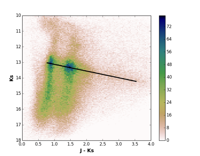
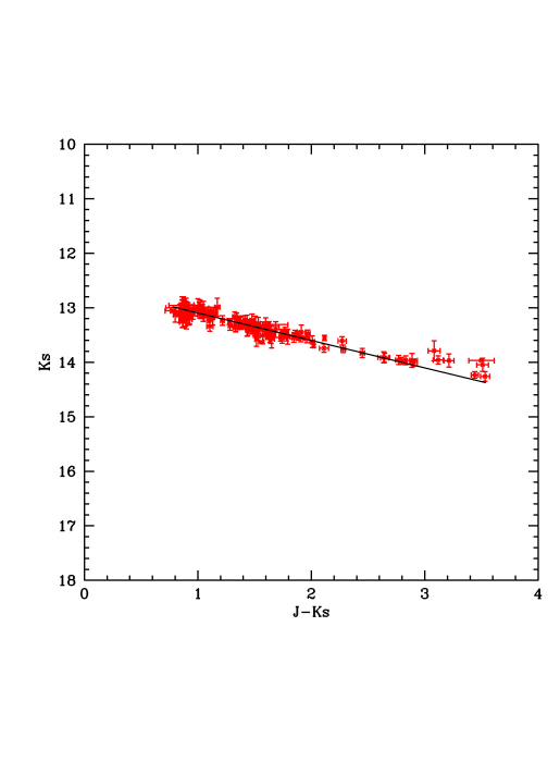
Рис. 1: (a) The color ($J-Ks$) – magnitude ($Ks$), diagram constructed for all stars from the VVV survey in the strip with coordinates and a width of $2\arcmin$. The number of stars in the histogram bins is marked by the color gradations on the scale rightward of the graph. (b) Observed magnitude of the RCG centroids localized in each of the $2\arcmin\times 2\arcmin$ strip regions versus color. The straight line on both panels indicates the linear model (1) that fits best the positions of the RCG centroids for the chosen sky strip.

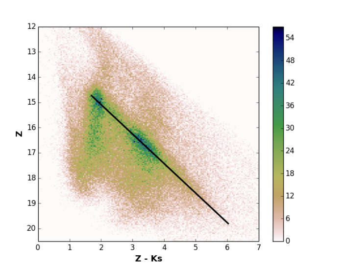
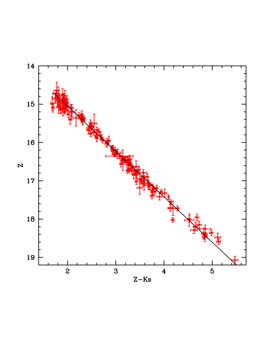
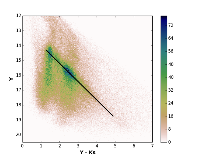
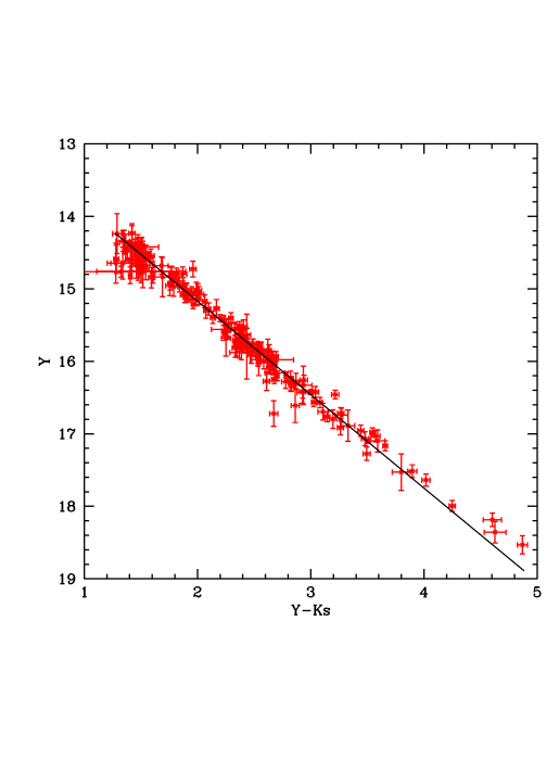
Рис. 2: Same as Fig. 1 for the ($Z,Ks$) and ($Y,Ks$) filters.

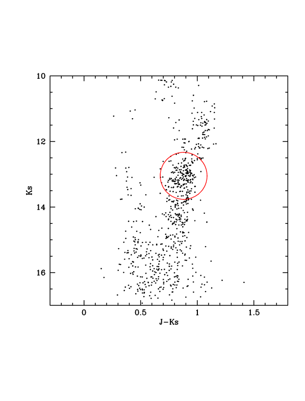
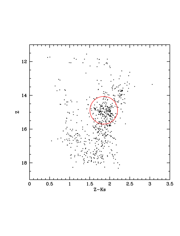
Рис. 3: An example of the color–apparent magnitude diagrams constructed in different filters for a $2\arcmin\times 2\arcmin$ cell of the sky strip under study from the VVV survey data. The circles schematically mark the RCG positions.

Thus, the technique for estimating the absolute $Z$ and $Y$ magnitude can be formulated as follows.

1. By investigating the chosen sky strip in the $J$ and $Ks$ filters, for which the absolute magnitudes of RCGs are known, we determine the distance to the bulge $D$ (pc) in a chosen direction from the following relations:

$$m_{Ks}=law_{JK}\times(J-Ks)+const_{JK},$$ (1)

$$5-5log_{10}D=M_{Ks}-law_{JK}\times(J-Ks)_{0}-const_{JK},$$ (2)

where $m_{Ks}$ is the observed Ks magnitude of the RCG centroid, ($J-Ks$) is the measured color, and Eq. (1) is the linear function that fits best the profile of the RCG branch in the strip under study.

2. By fitting the color–magnitude relation for the RCG centroids constructed in the ($Z,Ks$) and ($Y,Ks$) filters for all strip cells by a linear function, we obtain the corresponding slopes and constants. Using the previously derived distance $D$, we find absolute $Z$ and $Y$ magnitudes of RCGs, $M_{Z}$ and $M_{Y}$:

$$M_{Z}=(-law_{ZK}M_{Ks}+const_{ZK}+5--5log_{10}D)/(1-law_{ZK}),$$ (3)

$$M_{Y}=(-law_{YK}M_{Ks}+const_{YK}+5--5log_{10}D)/(1-law_{YK}).$$ (4)

As a result, for the chosen strip we obtain $m_{Ks}=0.43_{\pm 0.02}(J-Ks)+12.70_{\pm 0.02}$ (see Fig. 1), whence the extinction law determined by its slope immediately follows: $law_{JK}=A_{Ks}/E(J-Ks)=A_{Ks}/(A_{J}-A_{Ks})=0.43\pm 0.02$. It is important to note that this law differs noticeably from the standard $A_{Ks}/E(J-Ks)\approx 0.72$ (Cardelli et al. 1989), which is expectable for the bulge region and is consistent with the conclusions of previous papers (see Table 1 and, e.g., Popowski 2000; Udalski 2003; Sumi 2004; Nishiyama et al. 2009; Revnivtsev et al. 2010; Karasev et al. 2010a, 2010b; Nataf et al. 2016; Alonso-Garcia et al. 2017).

Таблица 1: Extinction laws obtained in this paper in comparison with the results of other authors

Extinction law	This paper	Cardelli et al. (1989)	Alonso-Garcia et al. (2017)
$A_{Z}/E(Z-Ks)$	$1.17\pm 0.02$	$1.3$	$1.15$
$A_{Y}/E(Y-Ks)$	$1.23\pm 0.01$	$1.44$	$1.23$
$A_{Ks}/E(J-Ks)$	$0.43\pm 0.02$	$0.72$	$0.428$

In addition, from the above relations we can esti- mate the distance modulus $5-5log_{10}D=-14.60\pm 0.04$ and the distance itself to the bulge in this part of the sky $D=8330\pm 150$ pc.

This result is important per se, and it agrees well with the present-day estimates of the distances to the central bulge regions (see, e.g., Bhardwaj et al. (2017) and references therein). Note that if we take $M_{Ks}=-1.63\pm 0.03$, derived by Gontcharov (2017) for relatively nearby stars as the reference absolute magnitude of RCGs, then we will obtain the estimate for the distance to the bulge as $D=8410\pm 150$ pc. It is consistent, within the measurement uncertainties, with the above value.

Repeating the above steps 1 and 2 for the color–observed magnitude diagram in the ($Z,Ks$) and ($Y,Ks$) filters, we obtain: $m_{Z}=1.17_{\pm 0.02}(Z-Ks)+12.75_{\pm 0.03}$ and $m_{Y}=1.23_{\pm 0.01}(Y-Ks)+12.74_{\pm 0.03}$ (Fig. 2), and from Eqs. (3) and (4) we determine $M_{Z}=-0.18\pm 0.43$ and $M_{Y}=-0.51\pm 0.30$.

To test our results, we investigated another strip farther from the Galactic center and located 12 away from the first one using the same technique. As a result, we obtained the following relations and values: $m_{Ks}=0.42_{\pm 0.03}(J-Ks)+12.73_{\pm 0.03}$, $m_{Z}=1.17_{\pm 0.02}(Z-Ks)+12.77_{\pm 0.03}$ and $m_{Y}=1.24_{\pm 0.01}(Y-Ks)+12.74_{\pm 0.02}$, whence from Eqs. (3) and (4) we determine $M_{Z}=-0.16\pm 0.45$ and $M_{Y}=-0.47\pm 0.29$.

We see that the results of our measurements for both strips agree between themselves much better than they could, given the so significant measurement errors. To conclude this section, recall that the above estimates were made by assuming the extinction law in the infrared filters to be weakly variable along the entire sky strip. The results of our measurements presented on the left panels of Figs. 1 and 2 and described by a simple linear model, on the whole, confirm this (the reduced value of $\chi^{2}\approx 1.2$). At the same time, it is worth noting that on these diagrams there are also points deviating significantly from the best-fit linear models. Their presence can be explained both by the existence of some local variations in the extinction law, which is quite possible even in sufficiently narrow strips (see, e.g., Gontcharov 2012; Nataf et al. 2013, 2016), and by the fact that the distance to the bulge RCGs along the strip can have some variability, and this variability will affect their observed magnitudes.

Thus, the proposed method yields the absolute magnitudes of RCGs, but their uncertainties are too large for these magnitudes to be used in subsequent studies. At the same time, this method allowed us to estimate the distance to the Galactic bulge quite accurately and to establish the extinction law (Table 1) that, even despite its possible local variations, is much better suited for the sky region under study than the standard one.

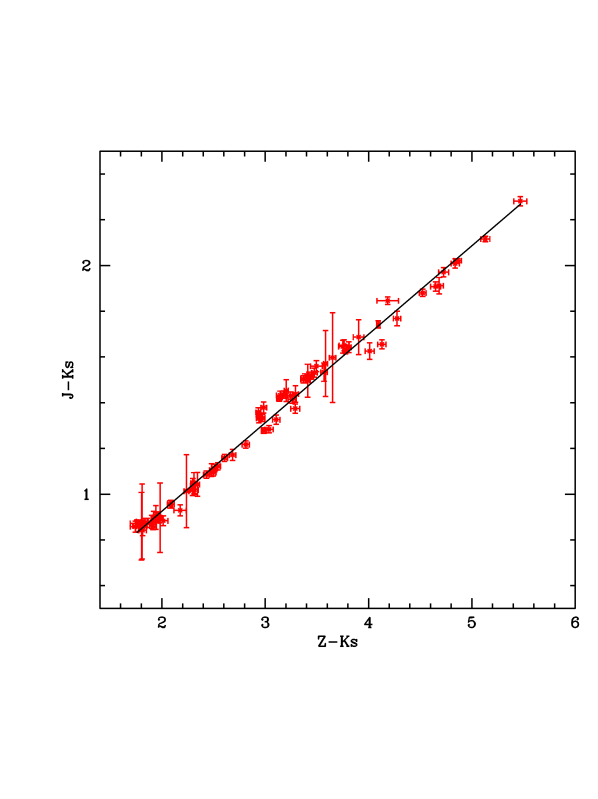
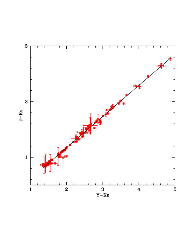
Рис. 4: (a) The color ($Z-Ks$) – color ($J-Ks$)’, diagram constructed for the strip with coordinates $l=1.7^{\circ}$, $b=[-5;5]$ from the VVV survey data. (b) The color ($Y-Ks$) – color ($J-Ks$), diagram constructed for the same sky region. The straight lines on both panels indicate the linear models that fit best the corresponding dependences.

3.2 The Second Method

We can attempt to reduce the measurement uncertainty of the absolute magnitudes determined in the previous section by combining and averaging the results for a large number of strips. However, in this approach we inevitably introduce an additional inaccuracy that is also related to the possible metallicity variations in the bulge (Gonzalez et al. 2015). If, however, we somehow specially select the strips, then the selection effect can manifest itself. Therefore, the approach that allows the absolute magnitudes to be reliably measured using only one strip is preferable.

Another way of reducing the final uncertainties is to use exclusively the observed colors of the RCG centroids, i.e., to use the $(J-Ks)-(Z-Ks)$ and $(J-Ks)-(Y-Ks)$ color–color diagrams (see Fig. 4) instead of the color–observed magnitude diagrams.

As a result of this approach, we obtain two sets of points that can be fitted by linear functions, $(J-Ks)=0.39_{\pm 0.01}(Z-Ks)+0.151_{\pm 0.015}$ and $(J-Ks)=0.56_{\pm 0.01}(Y-Ks)+0.05_{\pm 0.01}$. Given the intrinsic color $(J-Ks)_{0}$, we can determine the intrinsic colors $(Z-Ks)_{0}$ and $(Y-Ks)_{0}$ and the absolute magnitudes of RCGs as $M_{Z}=-0.25\pm 0.09$ and $M_{Y}=-0.485\pm 0.06$. These values are consistent with the results of the previous method but excel them noticeably in accuracy.

Note that abandoning the use of the observed magnitude of RCGs is also justified in that the natural scatter of RCG magnitudes is noticeably larger than the natural scatter of their colors (see below) and, therefore, it is more difficult to correctly determine the observed magnitude of RCGs than their color.

3.3 The Third Method

In the previous section we showed that abandoning the use of the observed magnitudes improved significantly the situation with errors in the derived absolute magnitudes, but they still remain fairly large. Furthermore, both methods described above suggest the constancy of the extinction law along the entire strip, but, as has already been noted above, the presence of its, even if fairly small, variations must not be ruled out completely. In this section we propose a method of indirectly estimating the absolute magnitudes in which only the colors of RCGs in the cell are used, but the assumption about the constancy of the extinction law along the entire strip is not required.

To determine the absolute $Z$ magnitude of RCGs ($M_{Z}$) by this method, only the strip cells in which the colors $(J-Ks)$ and $(Z-Ks)$ of RCGs were simultaneously measured are suitable for us. To determine $M_{Y}$, the cells in which the colors $(J-Ks)$ and $(Y-Ks)$ were simultaneously measured are suitable. Below we describe the algorithm for estimating the absolute magnitude in the $Z$ filter, but the same approach is also valid for other filters.

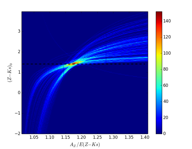
Рис. 5: Intrinsic color – extinction law diagram. The region with the greatest density of points (the largest number of intersections between the tracks of different cells) corresponds to the true value of the corresponding color (for more details, see the text). (a) For the extinction law $law_{JK}=A_{K}s/E(J-Ks)=0.43$. (b) For the extinction law $law_{JK}=0.5$. The dashed line marks the ordinate of the point of intersection between the tracks. The color gradation reflects the density of points on the diagram.

The observed color of RCGs depends on the intrinsic color and the relation between the extinctions:

$$(Z-Ks)=(Z-Ks)_{0}+(A_{Z}-A_{Ks}),$$ (5)

whence

$$(Z-Ks)_{0}=(Z-Ks)-A_{Z}+A_{Ks},$$ (6)

Thus, if we manage to determine the intrinsic colors of the RCG centroids in individual cells $(Z-Ks)_{0}=M_{Z}-M_{Ks}$ and $(Y-Ks)_{0}=M_{Y}-M_{Ks}$, then we will find the sought-for absolute magnitudes, because $M_{Ks}$ is known (see above). Obviously, the derived intrinsic colors in different cells must be the same (i.e., they must coincide, within the measurement uncertainties), because everywhere we are dealing with the properties of the same class of objects. Thus, $(Z-Ks)$ is a measurable quantity, the extinctions $A_{Z}$ and $A_{Ks}$ are related via the extinction law $law_{ZK}$ , and it only remains to determine $A_{Ks}$. This can be done by using the fact that we know the color $(J-Ks)$ of the RCG centroid in the same cell and the following relation:

$$(J-Ks)=(J-Ks)_{0}+(A_{J}-A_{Ks}),$$ (7)

where we know $(J-Ks)_{0}$, while $A_{J}$ and $A_{Ks}$ are related by the extinction law $law_{JK}=A_{Ks}/(A_{J}-A_{Ks})$.

Combining Eqs. (6) and (7), we find

$$(Z-Ks)_{0}=(Z-Ks)-\frac{law_{JK}}{(law_{ZK}-1)}\times\times((J-Ks)-(J-Ks)_{0}),$$ (8)

It can be seen from the derived formula that the entire dependence on extinction was reduced to the dependence on two extinction laws.

Let us now trace precisely how any variations in the extinction laws affect the derived absolute magnitude (or intrinsic color) in different cells. For this purpose, we will construct the true color – extinction law diagram (Fig. 5), where $law_{ZK}$ is along the horizontal axis and the intrinsic color $(Z-Ks)_{0}$ is along the vertical axis. To understand the dependence on the law $law_{JKs}$ , we will take two values: 0.43, i.e., the best-fit value from the previous section, and the arbitrary one 0.5. It can be seen from the figure that, depending on the extinction law $law_{ZK}$ , each of the strip cells forms its personal track on such a diagram, while changing the law $law_{JKs}$ simply shifted the entire picture of tracks along the horizontal axis.

It is clear from the diagram that the derived intrinsic colors must be reduced to some solution suitable for most of the cells. This solution is at the point (or the points, if there are RCGs with different absolute magnitudes in the chosen sky region) of intersection between the tracks, and the ordinate of the point of intersection will correspond to the sought-for intrinsic color. Moreover, it can be clearly seen from Fig. 5 that changing $law_{JKs}$ kept the ordinate of the point of intersection unchanged. Thus, if several extinction laws are present in the strip under study, then at an invariable absolute magnitude this will give rise to several points of intersection between the tracks with equal ordinates spaced along the horizontal axis apart.

Writing Eq. (8) for any two cells $i$ and $j$, we can show that the intrinsic color of RCGs (or, in other words, the projection of the point of intersection onto the vertical axis) does not depend on any of the extinction laws:

$$(Z-Ks)_{0}=(Z-Ks)_{i}-\frac{law_{JK}}{(law_{ZK}-1)}\times\times((J-Ks)_{i}-(J-Ks)_{0}),$$ (9)

$$(Z-Ks)_{0}=(Z-Ks)_{j}-\frac{law_{JK}}{(law_{ZK}-1)}\times\times((J-Ks)_{j}-(J-Ks)_{0}),$$ (10)

whence:

$$\frac{law_{JK}}{(law_{ZK}-1)}=\frac{(Z-Ks)_{j}-(Z-Ks)_{i}}{(J-Ks)_{j}-(J-Ks)_{i}},$$ (11)

and, finally,

$$(Z-Ks)_{0}=(Z-Ks)_{i}-\frac{(Z-Ks)_{j}-(Z-Ks)_{i}}{(J-Ks)_{j}-(J-Ks)_{i}}\times((J-Ks)_{i}-(J-Ks)_{0}).$$ (12)

Note that in contrast to the previous methods, where obtaining the result required assuming the extinction law to be invariable for the entire strip, here it is actually necessary to assume the equality of the extinction laws simultaneously only for two cells. Using Eqs. (9) – (12), we can now link all of the cells from the strip under consideration between themselves in pairs and find the sets of possible intrinsic colors of RCGs by investigating the density distribution of the points of intersection along the $(Z-Ks)_{0}$ axis.

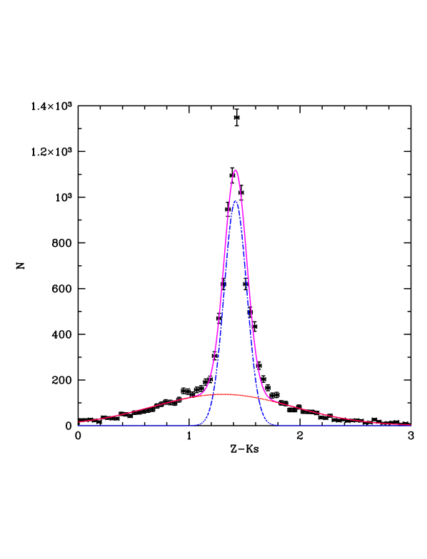
Рис. 6: The distribution of dereddened colors $(Z-Ks)_{0}$. The lines indicate the model that fits best the derived distribution (solid magenta line) and its components (dashed blue and dotted red lines).

The result of this approach is presented in Fig. 6. The only peak that corresponds to the intrinsic color of RCGs in the corresponding filters, which can be fitted by a Gaussian, is clearly seen. Besides, some broadening at the base of the distribution, which can be associated both with the statistical scatter of centroid points and with some variability of the extinction law in the strip, is noticeable. This broadening can be taken into account by adding an additional Gaussian component to the model. Note that if there were a sufficient number of RCGs with different absolute magnitudes in the strip, then several significant peaks would appear on the graph. Since this is not observed in our case, we can argue that RCGs of one type with the same (within the error limits) intrinsic color and absolute magnitude dominate in the sky region under study.

It is important to note that the derived color $(Z-Ks)_{0}$ is only one of the possible realizations, all of the measured quantities in Eq.(12) have their own measurement errors. Therefore, to determine the color $(Z-Ks)_{0}$ and its measurement error more properly, we used the so-called statistical bootstrap method. In this method each of the measured values is selected within the limits of its measurement error, whereupon Eqs. (9) – (12) are solved again, the derived distribution of $(Z-Ks)_{0}$ is fitted by a Gaussian, and its centroid is found. As a result of repeating such an analysis $\sim 30000$ times, we obtained a sample of $(Z-Ks)_{0}$ whose mean and dispersion determine the intrinsic color of RCGs and its measurement uncertainty, $(Z-Ks)_{0}=1.414\pm 0.025$ (Fig. 7). Note that the statistical bootstrap method is used quite widely in various problems of astrophysics, for example, to properly determine the measurement errors of the periods of X-ray pulsars (for a more detailed description, see Boldin et al. 2013).

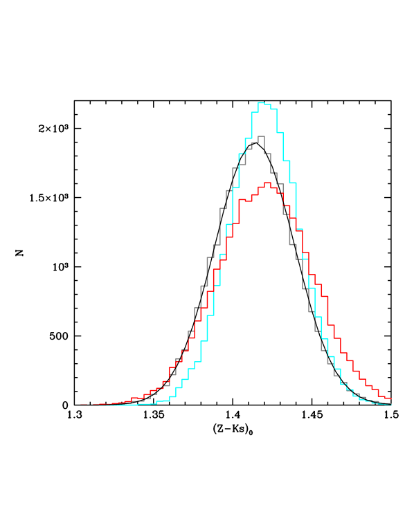
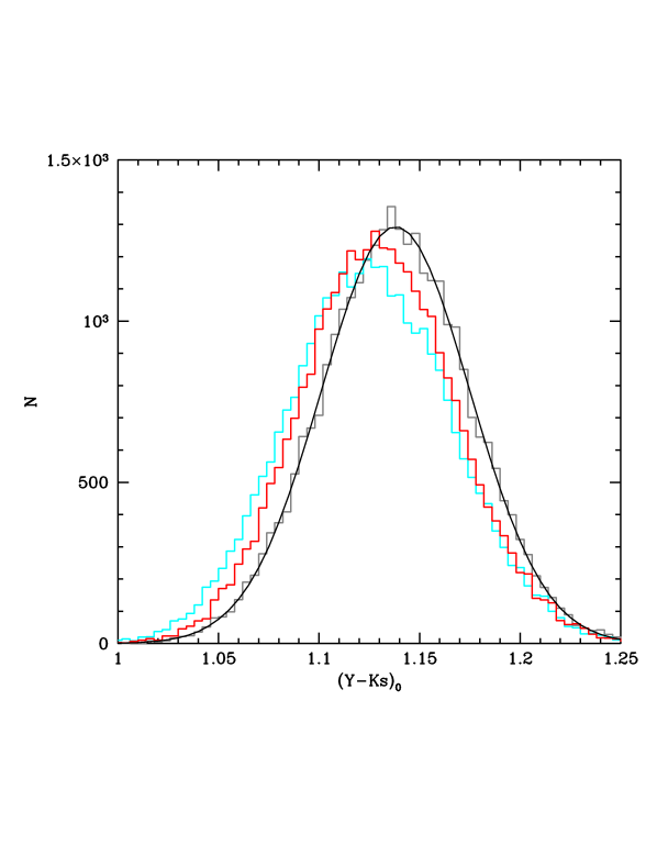
Рис. 7: The distribution of intrinsic colors $(Z-Ks)_{0}$ and $(Y-Ks)_{0}$, obtained by the statistical bootstrap method for three strips with a height $|b|<5^{\circ}$, perpendicular to the Galactic plane with the following longitudes: $l=1.7^{\circ}$ (black histogram), $l=0.1^{\circ}$ (red histogram), $l=2.37^{\circ}$ (blue histogram). As an example, the black solid line indicates the best-fit Gaussian model for the strip with $l=1.7^{\circ}$ (for more details, see the text).

Having measured the intrinsic color of RCGs for the $Z$-filter, we repeated the procedure described above and determined the true color in the $Y$-filter, $(Y-K)_{0}=1.137\pm 0.034$. Given the known $M_{Ks}$, we obtain the absolute magnitudes of RCGs $M_{Z}=-0.20\pm 0.04$ and $M_{Y}=-0.470\pm 0.045$, which are in good agreement with the results of previous sections, but excel them in accuracy.

The proposed method was applied not only for the strip in the vicinity of Baade’s window, but also for two more strips with coordinates l = $l=2.37^{\circ}$ and $l=0.1^{\circ}$. The latter passes in the immediate vicinity of the Galactic center, where the extinction is particularly great and manifestations of the inconstancy of the extinction law along the strip, if any, are possible. The results of our measurements of the intrinsic colors of RCGs and their absolute magnitudes with corresponding uncertainties are summarized in Table 2 for all three strips.

It can be seen from this table that the results of our measurements for all three strips agree well between themselves (the corresponding distributions of dereddened colors $(Z-Ks)_{0}$ and $(Y-K)_{0}$ are shown in Fig. 7).

Таблица 2: The intrinsic colors and absolute magnitudes of RCGs determined for the sky strips in different parts of the bulge

$l$	$(Z-Ks)_{0}$	$(Y-Ks)_{0}$	$M_{Z}$	$M_{Y}$
$1.7^{\circ}$	$1.414\pm 0.025$	$1.137\pm 0.034$	$-0.20\pm 0.04$	$-0.470\pm 0.045$
$2.37^{\circ}$	$1.419\pm 0.025$	$1.130\pm 0.032$	$-0.19\pm 0.04$	$-0.480\pm 0.044$
$0.1^{\circ}$	$1.420\pm 0.027$	$1.129\pm 0.035$	$-0.19\pm 0.04$	$-0.481\pm 0.046$

To finally demonstrate the operability and properness of the method, we attempted to determine the absolute magnitudes of RCGs for the filters in which they are already well known. Since the corresponding magnitudes for the $Ks$ and $J$ filters are a necessary part of our analysis and cannot be derived based on themselves, we chose the $H$ filter for our test. As a result of repeating the procedure described above for the strip in the vicinity of Baade’s window, we determined the absolute magnitude of RCGs in this filter, $M_{H}=-1.50\pm 0.03$, that in good agreement with $M_{H}=-1.490\pm 0.015$ obtained by Laney et al. (2012) and $M_{H}=-1.49\pm 0.04$ measured by Gontcharov (2017).

4 THE ABSOLUTE MAGNITUDES OF BULGE RED CLUMP GIANTS IN THE IRAC/SPITZER FILTERS

Having made sure that the proposed technique is operable for the filters of the VISTA surveys, we used it to determine the absolute magnitudes of RCGs in the filters of the IRAC/Spitzer survey. The study was performed in the same three sky strips for which the absolute $Z$ and $Y$ magnitudes were obtained above. Note that the range of Galactic latitudes covered by the GLIMPSE/Spitzer surveys is slightly smaller than the corresponding coverage of the VVV/VISTA survey, but the number of cells ($170-210$) in each of the strips turned out to be enough to solve our problems.

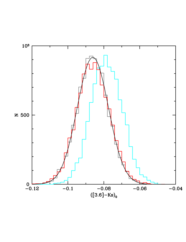
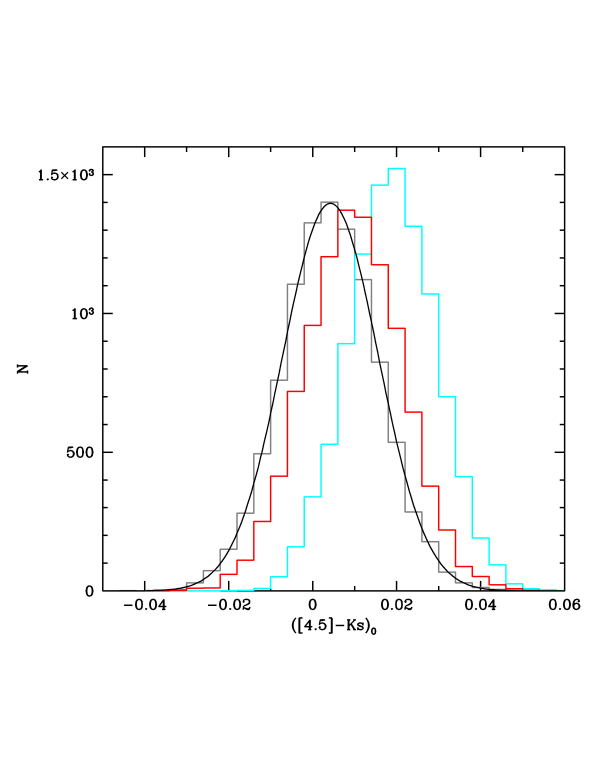
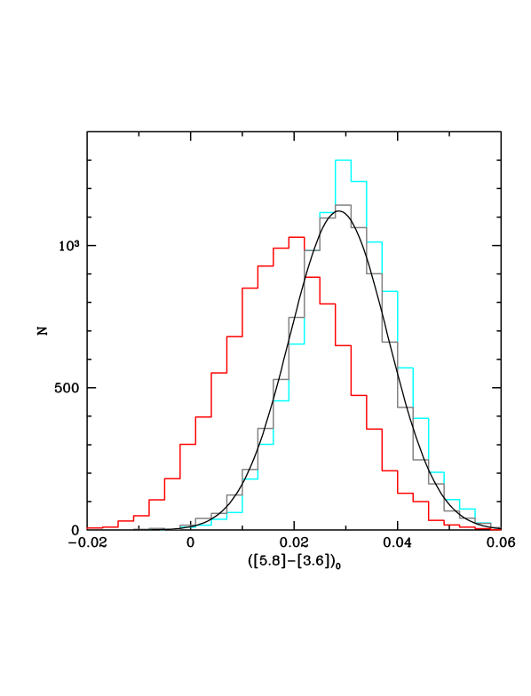
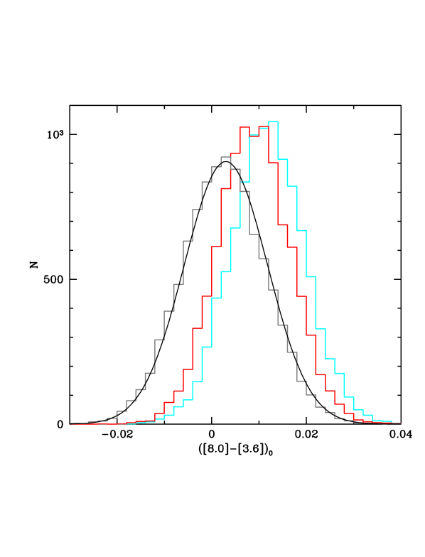
Рис. 8: Same as Fig. 7 for the GLIMPSE/Spitzer filters.

To find the absolute magnitudes of RCGs in the $[3.6]$ and $[4.5]$ filters, as above, we used the known absolute $Ks$ and $J$ magnitudes and the VVV survey data in these filters as the basic ones. Therefore, we first cross-correlated the VVV (DR4) and GLIMPSE catalogues to select the stars with a statistically significant detection in both catalogues. Then, we determined the colors $([3.6]-Ks)$ and $([4.5]-Ks)$ (the color $J-Ks$ was determined previously) of the RCG centroids in the strip cells and used the third method to determine the intrinsic colors $([3.6]-Ks_{0})$ and $([4.5]-Ks)_{0}$. To find the centroid and to refine the errors, as in the previous section, we used the statistical bootstrap method, except that the number of selected values was 10 000. The corresponding distributions are shown in Fig. 8 (upper panels).

As a result of our analysis, we measured the absolute magnitudes of RCGs in the $[3.6]$ and $[4.5]$ filters: $M_{[3.6]}=-1.70\pm 0.03$ and $M_{[4.5]}=-1.60\pm 0.03$.

To determine the absolute magnitudes in the $[5.8]$ and $[8.0]$ filters, we used the above results of our measurements of the absolute magnitude in the $[3.6]$ filter. This is because we managed to determine the colors $([5.8]-[3.6])$ and $([8.0]-[3.6])$ for RCGs more accurately than the colors $([5.8]-Ks)$ and $([8.0]-Ks)$. Therefore, the third method of determining the absolute magnitude was applied to these colors and the color $(J-[3.6])$ as the reference one. The distributions of intrinsic colors $([5.8]-[3.6])_{0}$ and $([8.0]-[3.6])_{0}$ are shown in Fig. 8 (lower panels), while the absolute magnitudes of RCGs in the $[5.8]$ and $[8.0]$ filters are $M_{[5.8]}=-1.67\pm 0.03$ and $M_{[8.0]}=-1.70\pm 0.03$, respectively. It can be seen from the figure that, as above, the results for different strips agree well between themselves, within the uncertainties.

It is also worth noting that in the $[5.8]$ and $[8.0]$ filters of the GLIMPSE survey RCGs are recorded at the detection limit. Therefore, we admit the presence of a noticeable admixture of branch giants in our sample, which can be responsible for some additional systematic error in the derived magnitudes in these filters. However, if we look at the isochrones from the PARSEC database, then we can understand that the maximum systematic error in the colors used in our study is small and does not exceed 0.01 mag.

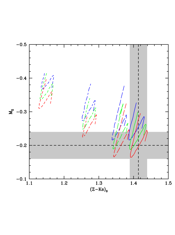
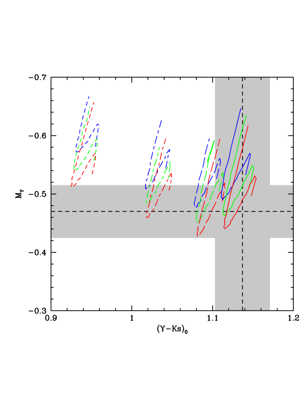
Рис. 9: The isochrones for RCGs of different metallicities (${\bf Z}=0.00744,{\bf Z}_{\sun}=0.0152,{\bf Z}=0.0276,{\bf Z}=0.038$, from left to right) and ages (the red, green, and blue lines for 10, 9, and 8 Gyr, respectively) constructed using the PARSEC database for the $Z$ filter and color $Z-Ks$ (a) and for the $Y$ filter and color $Y-Ks$ (b). In the construction we assumed that there was no interstellar extinction. The black dashed lines mark our absolute values and intrinsic colors. The gray shading indicates the errors corresponding to one standard deviation for the corresponding magnitudes. The solid lines highlight the isochrones that correspond best to the observed $Z$ magnitudes.

5 DISCUSSION

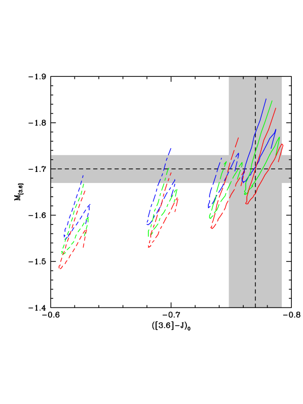
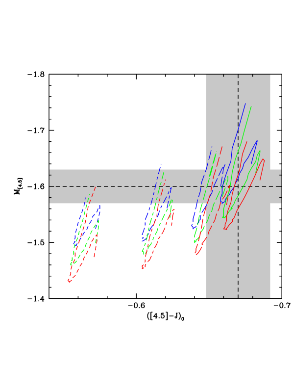
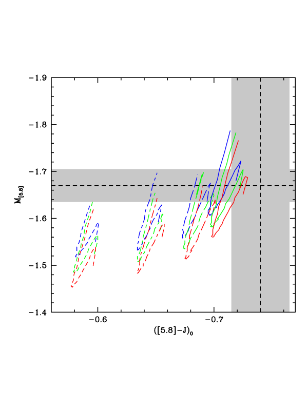
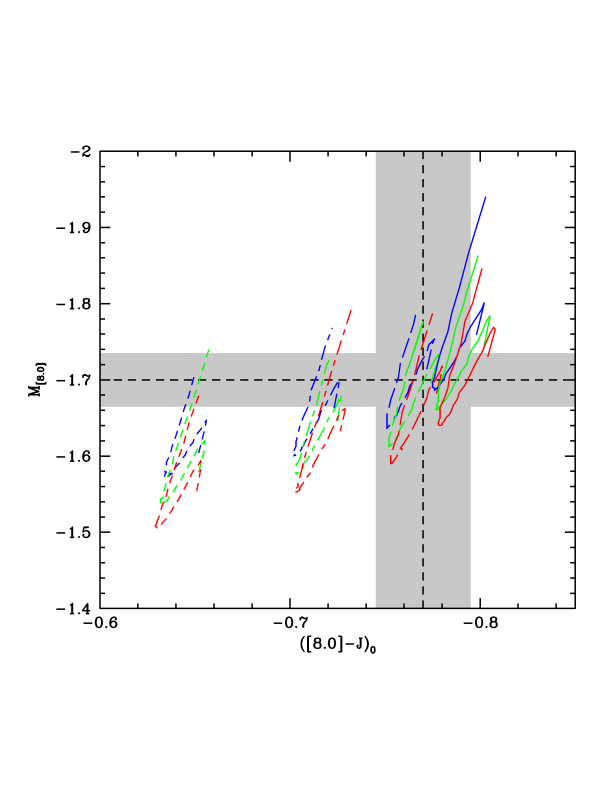
Рис. 10: Same as Fig. 9 for the GLIMPSE/Spitzer filters.

To understand how well our absolute magnitudes of RCGs agree with theoretical models, we compared them with the PARSEC isochrones constructed for the ages and metallicities typical of bulge RCGs. We chose the isochrones for RCGs of three ages, 8, 9, and 10 Gyr (see, e.g., Zoccali et al. 2003; Vanhollebeke et al. 2009), and two metallicities from Gonzalez et al. (2015) – $[Fe/H]\simeq-0.40$ (the low-metallicity subgroup of RCGs) and $[Fe/H]\simeq 0.26$ (the high-metallicity subgroup of RCGs), as well as the solar metallicity (abundance). Since a different parametrization of the metallicity (${\bf Z}$) is used in the PARSEC database and the isochrones normalized to the solar abundance are presented, below we adopt $[M/H]=[Fe/H]$. In this case, $[M/H]$ were recalculated to Z using the formula $[M/H]=log_{10}({\bf Z}/{\bf Z_{\sun}})$ by assuming ${\bf Z}_{\sun}=0.0152$, according to the recommendations of the PARSEC database. Thus, the above metallicities from Gonzalez et al. (2015) correspond to ${\bf Z}=0.00744$ and ${\bf Z}=0.0276$. The results of the comparison of the isochrones and our measurements are shown in Figs. 9 and 10.

It can be seen that our absolute magnitudes in all filters agree with the theoretical models for high- metallicity RCGs. Moreover, if add the intrinsic colors of RCGs in different filters to our analysis, then additional constraints on the metallicity of bulge RCGs can be obtained. In particular, to correspond to the measured values within one standard deviation, their metallicity must be $[M/H]\simeq 0.4$ (${\bf Z}=0.038$) with an uncertainty no greater than $0.1dex$. Although this is formally slightly larger than that in Gonzalez et al. (2015), it agrees with the estimates of the latter within the error limits.

It can also be seen from the comparison of the derived magnitudes with the isochrones that objects with an age of 9–10 Gyr, with the possible inclusion of younger objects with an age of $\sim$8 Gyr, must dominate among the bulge RCGs. The $Z$ filter close to the optical band, which allows the most accurate estimates to be obtained, is most revealing in this regard. The measurements in the $Y$ , [3.5], and [4.5] filters also agree well with the above estimates; the results for the more distant [5.6] and [8.0] filters give less accurate agreement, but they are consistent within the measurement uncertainty limits.

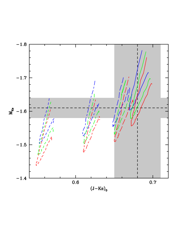
Рис. 11: Same as Fig. 9 for the J and Ks filters.

Note that the natural scatter of RCG colors following from the PARSEC isochrones is comparable to our standard deviations for the colors of these objects, i.e., our estimates correspond in accuracy to the "natural"accuracy (the scatter of colors) typical for RCGs.

It is interesting to check how well the absolute magnitudes of RCGs in the J and Ks filters, which we everywhere used as the reference ones, agree with our metallicity estimates. Using the PARSEC data, we constructed the isochrones for RCGs of three ages and four metallicities (as above) in these filters (Fig. 11). It follows from the figure that the reference values for RCGs in the $J$ and $Ks$ filters agree excellently with the theoretical expectations for our metallicity. The metallicity $[Fe/H]\simeq 0.26$ from Gonzalez et al. (2015) is also consistent with our results and falls into the range of measurement errors.

Using the estimated absolute magnitudes of RGCs and their metallicities, we checked how well our results agreed with the stellar atmosphere models for these objects. For this purpose, we converted the derived magnitudes to the flux densities and compared them with the spectra of red giants with temperatures from $\sim$4000 to $\sim$4750 K (this choice is explained by the universally accepted view of RCG temperatures; see, e.g., Girardi 2016) generated with the SYNPHOT package for synthetic photometry and the Kurucz library of spectra for ${\bf Z}=0.038$ and ${\bf Z}=0.0152$ (solar abundance). The result of such a comparison is shown in Fig. 12. We used the relations from Cohen et al. (2003) to convert the $J$, $H$, $Ks$ magnitudes and the relations at the official VISTA site (they were first reduced to the AB system using the corresponding coefficients) to convert the $Z$ and $Y$ magnitudes. To convert the Spitzer magnitudes, we used the resource and conversion tools at the Gemini site.

It can be seen that our results agree well with the assumptions about the temperature properties of red giants. Moreover, using the estimates for the metallicity of these stars obtained above, we can determine the most suitable temperature for the RCGs under study, $4250\pm 150$ K (Fig. 12).

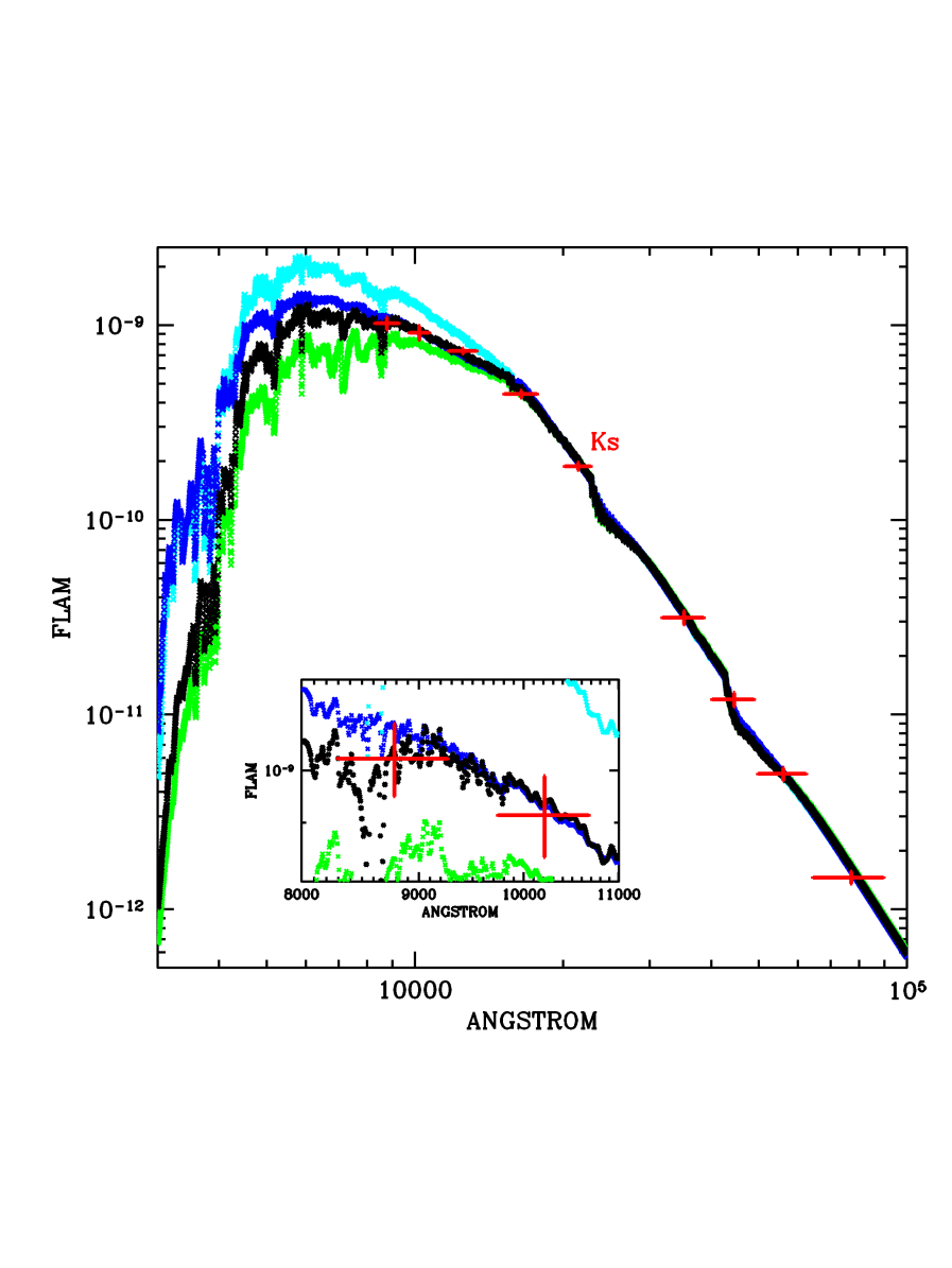
Рис. 12: The synthetic spectra constructed for red giants with temperatures of $4000$ K (green curve), $4250$ K (black curve), $4750$ K (blue curve) for metallicity ${\bf Z}=0.038$, and $4400$ K for the solar abundance ${\bf Z}=0.0152$ (blue curve) using the SYNPHOT package and the Kurucz library of spectra. The spectra were normalized to the absolute $Ks$ magnitude of RCGs. The crosses indicate the fluxes corresponding to the absolute magnitudes of RCGs in nine infrared filters: $Z,Y,J,H,Ks,[3.6],[4.5],[5.8]and[8.0]$ (from left to right), including those measured in this paper. A magnified part of the main picture near the $Z$ and $Y$ filters is presented in a separate inset.

6 CONCLUSIONS

In this paper for the first time we have determined the absolute magnitudes of bulge red clump giants in the infrared $Z$ and $Y$ filters of the VVV (VISTA/ESO) survey and the [3.6], [4.5], [5.8], and [8.0] bands of the GLIMPSE (IRAC/Spitzer) Galactic-plane survey. Our results are based on the use of narrow vertical strips to determine the colors of RCGs in different filters and the extinction law. This method was proposed by Karasev et al. (2015) and developed further in this paper.

The results obtained in this paper (the absolute magnitudes, the corresponding flux densities, and their standard deviations) are presented in Table 3.

A comparison of the derived absolute magnitudes with theoretical models allowed us to measure the metallicity of bulge RCGs, $[M/H]\sim 0.40$ (or ${\bf Z}\sim 0.038$) with an error of $[M/H]\sim 0.1$ dex, and their characteristic temperature, $\sim 4250\pm 150$ K. We also showed that stars with an age of 9 – 10 Gyr dominate among RCGs, but, at the same time, younger objects with an age of $\sim$8 Gyr may also be present.

Таблица 3: Parameters of the photometric bands under study and the absolute magnitudes of bulge RCGs

Filter	$\lambda_{eff},$ Å	$\omega,$ Å	$M$, mag	FLAM, erg cm-2 s -1 Å-1
$Z_{Vista}$	8762.58	970	$-0.20\pm 0.04$	$1.024_{\pm 0.07}\times 10^{-09}$
$Y_{Vista}$	10239.64	930	$-0.470\pm 0.045$	$9.14_{\pm 0.74}\times 10^{-10}$
$[3.6]_{Spitzer}$	35242.46	6836	$-1.70\pm 0.03$	$3.15_{\pm 0.24}\times 10^{-11}$
$[4.5]_{Spitzer}$	44540.45	8649	$-1.60\pm 0.03$	$1.20_{\pm 0.11}\times 10^{-11}$
$[5.8]_{Spitzer}$	56095.61	12561.17	$-1.67\pm 0.03$	$4.96_{\pm 0.37}\times 10^{-12}$
$[8.0]_{Spitzer}$	77024.24	25288.50	$-1.70\pm 0.03$	$1.46_{\pm 0.1}\times 10^{-12}$
$H$	16372.50	2510	$-1.50\pm 0.03$	$7.37_{\pm 0.22}\times 10^{-10}$

It is important to note the absence of noticeable differences in the absolute magnitudes derived for strips in different parts of the Galactic bulge. This may suggest that the metallicity in the vicinity of the Galactic center differs only slightly from the metallicity near Baade’s window. In addition, good agreement between the absolute magnitudes of RCGs (primarily in the $Y$ filter) obtained by different methods, including those assuming the constancy of the distance and extinction law along the entire strip, is worth noting. This may suggest that the extinction law is highly constant within the chosen strips perpendicular to the Galactic plane. On the other hand, the infrared filters may simply less sensitive to small variations in this law (Nataf et al. 2013, 2016).

We also showed that toward the sky regions under study the extinction law differs noticeably from the standard one, and its allowance is very important for obtaining the correct estimates of the absolute magnitudes. In addition, we estimated the distances to several Galactic bulge regions, – $D=8200-8500$ pc, in good agreement with the results of other papers.

REFERENCES

1. D.R. Alves, ApJ539, 732 (2000).

2. J. Alonso-Garcia, D. Minniti, M. Catelan, R. Ramos, O. Gonzalez, M. Hempel, P. Lukas, R. Saito, et al, arXiv:1710.04854v1 (2017).

3. T.-L. Astraatmadja and C.A.L. Bailer-Jones , ApJ833, 119 (2016).

4. Boldin P.A., Tsygankov S.S., Lutovinov A.A., Astron. Lett. 39, 375 (2013).

5. T. Bensby, J.C. Yee, S. Feltzing, J.A. Johnson, A. Gould, J.G.Cohen, M. Asplund, J. Melendez, et al., A&A549, 147 (2013).

6. A. Bressan, P. Marigo, L. Girardi, B. Salasnich, C. Dal Cero, S. Rubele, A. Nanni, MNRAS 427, 127 (2012), http://stev.oapd.inaf.it/cmd.

7. A. Bhardwaj, M. Rejkuba, D. Minniti, F. Surot, E. Valenti, M. Zoccali, O. A. Gonzalez, M. Romaniello, et al, A&A605, id.A100 (2017).

8. E. Vanhollebeke, M. A. T Groenewegen, L. Girardi, A&A498, 95 (2009).

9. O. Gerhard, Martinez-Valpuesta, Astrophys. J. Letters 744, L8, (2012).

10. O. A. Gonzalez, M. Rejkuba, M. Zoccali, E. Valenti, D. Minniti, M. Schultheis, R. Tobar, B. Chen, A&A552, 9 (2012).

11. O. A. Gonzalez, M. Zoccali, S. Vasquez, V. Hill, M. Rejkuba, E. Valenti, A&A584, A46, (2015).

12. Gontcharov G.A., Astron. Lett. 34, 785 (2008).

13. Gontcharov G.A., Astron. Lett. 38, 12 (2012).

14. Gontcharov G.A. and Baykova A.T., Astron. Lett. 39, 689 (2013).

15. Gontcharov G.A., Astron. Lett. 43, 545, (2017).

16. C.M. Dutra, B.X. Santiago, E.L.D. Bica, B. Barbuy, MNRAS 338, 253 (2003).

17. Leo Girardi, MNRAS 308, 818-832 (1999).

18. Leo Girardi, Ann. Rev. Astron. Astrophys. 54, p.95-133 (2016).

19. M. Zoccali, A. Renzini, S. Ortolani, L. Greggio, I. Saviane, S. Cassisi, M. Rejkuba, B. Barbuy, R. M. Rich and E. Bica, A&A399, 931 (2003).

20. Karasev, D. I., Lutovinov, A. A., Burenin , R. A., MNRAS Lett. 409, L69 (2010a).

21. Karasev, D. I., Revnivtsev, M. G., Lutovinov, A. A., Burenin, R. A., Astron. Lett. 36, 788 (2010b).

22. Karasev, D. I., Tsygankov, S. S., Lutovinov, A. A., Astron. Lett. 41, 394 (2015).

23. J.A. Cardelli, G.C. Clayton and J.S. Mathis, ApJ345, 245 (1989).

24. M. Cohen, Wm. A. Wheaton, S. T. Megeath, ApJ126, 1090 (2003).

25. C. D. Laney, M. D. Joner, G. Pietrzy’nski, MNRAS 419, Issue 2 (2012).

26. P. Marigo, L. Girardi, A. Bressan, Philip Rosenfield, Bernhard Aringer, Yang Chen, Marco Dussin, Ambra Nanni, et al, ApJ835, 77 (2017).

27. D. M. Nataf, A. Gould, P. Fouque’, O. A. Gonzalez, J. A. Johnson, J. Skowron, A. Udalski, M. K. Szymanski, et al , ApJ769, 88 (2013).

28. D. M. Nataf, O. A. Gonzalez, L. Casagrande, G. Zasowski, C. Wegg, C. Wolf, A. Kunder, J. Alonso-Garcia, et al., MNRAS 456, 2692 (2016).

29. S. Nishiyama, M. Tamura, H. Hatano, D. Kato, T. Tanabe, K. Sugitani, T. Nagata, ApJ696, 1407 (2009).

30. B. Paczynski and K. Stanek, A&A494, 219 (1998).

31. P. Popowski, ApJ528, 9 (2000).

32. Revnivtsev, M., van den Berg, M., Burenin, R., Grindlay, J. E., Karasev, D., Forman, W., A&A515, A49 (2010).

33. T. Sumi, MNRAS 349, 193 (2004).

34. A. Udalski, ApJ590, 284 (2003).

Translated by V. Astakhov