Asteroseismic modelling of solar-type stars: internal systematics from input physics and surface correction methods

Abstract

Asteroseismic forward modelling techniques are being used to determine fundamental properties (e.g. mass, radius, and age) of solar-type stars. The need to take into account all possible sources of error is of paramount importance towards a robust determination of stellar properties. We present a study of 34 solar-type stars for which high signal-to-noise asteroseismic data is available from multi-year Kepler photometry. We explore the internal systematics on the stellar properties, that is, associated with the uncertainty in the input physics used to construct the stellar models. In particular, we explore the systematics arising from: (i) the inclusion of the diffusion of helium and heavy elements; and (ii) the uncertainty in solar metallicity mixture. We also assess the systematics arising from (iii) different surface correction methods used in optimisation/fitting procedures. The systematics arising from comparing results of models with and without diffusion are found to be 0.5%, 0.8%, 2.1%, and 16% in mean density, radius, mass, and age, respectively. The internal systematics in age are significantly larger than the statistical uncertainties. We find the internal systematics resulting from the uncertainty in solar metallicity mixture to be 0.7% in mean density, 0.5% in radius, 1.4% in mass, and 6.7% in age. The surface correction method by Sonoi et al. and Ball & Gizon’s two-term correction produce the lowest internal systematics among the different correction methods, namely, $\sim$1%, $\sim$1%, $\sim$2%, and $\sim$8% in mean density, radius, mass, and age, respectively. Stellar masses obtained using the surface correction methods by Kjeldsen et al. and Ball & Gizon’s one-term correction are systematically higher than those obtained using frequency ratios.

1 Introduction

Our knowledge of the underlying physical processes taking place in deep stellar interiors is of great importance for the accurate characterization of stars and classification of stellar populations. The treatment and choice of the essential model input physics such as solar metallicity mixture (Grevesse & Sauval, 1998; Asplund et al., 2009; Lodders & Palme, 2009), initial helium abundance (Chiosi & Matteucci, 1982; Casagrande et al., 2007), as well as the different mixing processes like convection, semi-convection, convective overshooting (Monteiro et al., 1996; Christensen-Dalsgaard et al., 2011; Deheuvels & Michel, 2011; Piau et al., 2011; Silva Aguirre et al., 2011; Trampedach & Stein, 2011), microscopic diffusion, radiation levitation, and rotational mixing (Thoul et al., 1994; Turcotte et al., 1998; Maeder & Meynet, 2000) have a direct impact on the derived stellar parameters such as mass, radius, and age.

In order to aid the characterization of extra-solar planetary systems, current efforts are being geared towards improving the synergies between planetary science and asteroseismology (see, e.g. the book by Campante et al. 2017). Asteroseismology has proven to be an effective technique in determining precisely the exoplanet-host star parameters and hence planet properties (Huber et al., 2013; Benomar et al., 2014; Marcy et al., 2014; Campante et al., 2015, 2016a). Transit observations can only provide an estimate of the planet-to-star radius ratio. Therefore, precise stellar radii from asteroseismology allow tight constraints to be placed on the absolute sizes of planets. For bright enough systems, radial-velocity observations may be combined with the transit data to estimate planetary masses. The inferred planetary mass scales with the stellar mass according to $M_{\rm p}\propto M^{2/3}$ (e.g. Perryman, 2014) which asteroseismology can again provide (Campante et al., 2017). Last but not least, stellar ages from asteroseismology can potentially be used to assess the dynamical stability of planetary systems and to establish their relative chronology.

Photometric observations by NASA’s Kepler space telescope (Borucki et al., 2010) led to the characterization of several hundred solar-type stars using asteroseismology. Future space missions such as NASA’s Transiting Exoplanet Survey Satellite (TESS; Campante et al., 2016b) will allow the detection of oscillations in up to 10,000 solar-type stars with low temporal resolution, whereas ESA’s PLAnetary Transits and Oscillations of stars mission (PLATO; Rauer et al., 2014) is expected to reach $\sim$80,000 solar-type stars with detected oscillations based on multi-year observations. With this in mind, efforts are being directed towards increasing the precision of asteroseismic inferences by matching the observed oscillation frequencies (or their combinations) to the corresponding frequencies (or their combinations) obtained from the stellar evolutionary models (Miglio & Montalbán, 2005; Metcalfe et al., 2012, 2014; Silva Aguirre et al., 2013, 2015; Davies et al., 2016). This approach is known to improve the precision of derived stellar parameters over forward modelling methods that only consider global oscillation parameters (i.e. the frequency of maximum oscillation power, $\nu_{\rm max}$, and the large frequency separation, $\Delta\nu$; Mathur et al., 2012; Lebreton & Goupil, 2014). It nevertheless yields stellar parameters that are model-dependent and therefore sensitive to the input physics used in the models. For instance, the estimated stellar ages are sensitive to different transport processes such as microscopic diffusion, convection and overshooting, which need to be parameterized. Consequently, the treatment of the input physics becomes a source of uncertainty that cannot be easily accounted for.

Silva Aguirre et al. (2015) compared stellar properties of 33 Kepler planet-candidate host stars derived using a variety of stellar evolutionary codes and optimisation/fitting methods, yielding internal systematics of $\sim$1% in radius and density, $\sim$2% in mass, and $\sim$7% in age. In order to avoid internal systematics arising from the adoption of a variety of evolution and optimisation tools, we employ the same tools in all computations performed in this work. This paper is then aimed at exploring systematic effects arising from specific choices of the input physics used in models of solar-type stars. In particular, we explore internal systematics arising from the inclusion of diffusion in model grids and changes in element abundances. Inclusion of atomic diffusion in stellar models and its impact on the derived stellar parameters has been the subject of a number of studies over the past decades (Aller & Chapman, 1960; VandenBerg et al., 2002; Dotter et al., 2017). This is mainly because atomic diffusion has been revealed to occur in the Sun and other stars (Guzik & Cox, 1993; Christensen-Dalsgaard et al., 1993; Korn et al., 2007). We also explore the internal systematics arising from the uncertainty in the solar metallicity mixture. Different solar metallicity mixtures (e.g. Grevesse & Sauval, 1998; Asplund et al., 2009) are being adopted in stellar modelling tools despite differences in the absolute element abundances (Miglio & Montalbán, 2005; Serenelli & Basu, 2010; Silva Aguirre et al., 2015, 2017). This hence becomes a potential source of uncertainty in the derived stellar parameters. Furthermore, we assess the internal systematics arising from commonly used surface correction methods. Ball & Gizon (2017) investigated the performance of different surface correction methods applied to evolved stars (i.e. subgiants and low-luminosity red giants) and established the total additional uncertainties in the derived radii, masses, and ages to be less than 1%, 2%, and 6%, respectively. In this paper, we assess the performance of different surface correction methods by comparing them with the use of frequency ratios, known to be less prone to near-surface effects (Roxburgh & Vorontsov, 2003).

This paper is organised as follows. In Sect. 2, we describe our target sample, as well as the adopted seismic and spectroscopic observables. In Sect. 3, we present the stellar evolution code, the different model grids, and the optimisation procedure used, while the main results are discussed in Sect. 4. Section 5 presents a summary of our findings.

2 Target Sample

Our sample consists of 34 solar-type oscillators which have been observed by the Kepler satellite. Of these, 32 stars are part of the ‘LEGACY’ sample (Lund et al., 2017; Silva Aguirre et al., 2017) with the remaining 2 stars being the components of the asteroseismic binary HD 176465 (White et al., 2017; Nsamba et al., 2017). These stars were observed in Kepler short-cadence mode ($\Delta t=58.89\>{\rm s}$) for at least 12 months. The sample includes some of the highest signal-to-noise ratio, solar-like oscillators observed by Kepler. Details about light curve preparation, power spectrum calculation, the peak-bagging procedure and adopted individual oscillation frequencies are given in Lund et al. (2017).

The target sample is shown in an asteroseismic Hertzsprung–Russell diagram in Fig. 1. The adopted $\Delta\nu$ is from Lund et al. (2017), computed following a Gaussian-weighted linear fit to $l=0$ mode frequencies expressed as a function of the radial order. Most of the stars in the target sample are more evolved than the Sun.

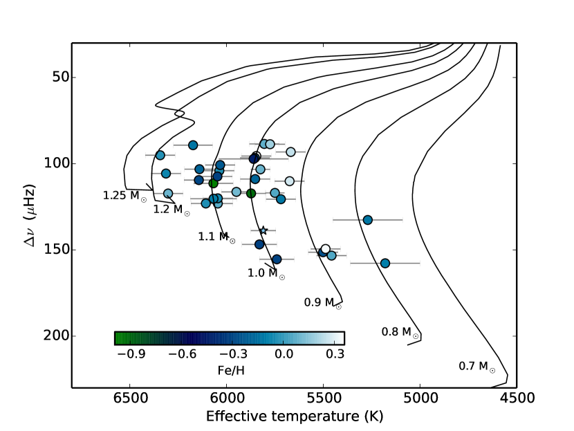
Figure 1: Target sample. Stellar evolutionary tracks were constructed at solar metallicity and range in mass from 0.7 to 1.25 M_⊙. Stars are colour-coded according to their metallicities. The ‘star’ symbol corresponds to the position of the Sun.

Table 1 contains the atmospheric properties of the stars in our sample. Most of the spectroscopic parameters were retrieved from Lund et al. (2017). These classical constraints will complement the asteroseismic parameters in the optimisation procedure (as described in Sect. 3). The components of the binary HD 176465 (White et al., 2017) have effective temperatures $5830\pm 90\>{\rm K}$ (HD 176465 A) and $5740\pm 90\>{\rm K}$ (HD 176465 B), and similar metallicity ($-0.30\pm 0.06\>{\rm dex}$). our

Table 1: Spectroscopic parameters of sample stars. The effective temperature ($\rm T_{\rm eff}$) and metallicity ([Fe/H]) are adopted from ^aCasagrande et al. (2014), ^bPinsonneault et al. (2012),^cPinsonneault et al. (2014), and ^dRamírez et al. (2009) as indicated. The remaining parameters are from Lund et al. (2017).

KIC	$T_{\mbox{eff}}$ (K)	[Fe/H] (dex)
3427720	6045 $\pm$ 77	-0.06 $\pm$ 0.10
3656476	5668 $\pm$ 77	0.25 $\pm$ 0.10
3735871	6107 $\pm$ 77	-0.04 $\pm$ 0.10
4914923	5805 $\pm$ 77	0.08 $\pm$ 0.10
5184732	5846 $\pm$ 77	0.36 $\pm$ 0.10
5950854	5853 $\pm$ 77	-0.23 $\pm$ 0.10
6106415	6037 $\pm$ 77	-0.04 $\pm$ 0.10
6116048	6033 $\pm$ 77	-0.23 $\pm$ 0.10
6225718	6313 $\pm$ 77	-0.07 $\pm$ 0.10
6603624	5674 $\pm$ 77	0.28 $\pm$ 0.10
7106245	6068 $\pm$ 102a	-0.99 $\pm$ 0.19a
7296438	5775 $\pm$ 77	0.19 $\pm$ 0.10
7871531	5501 $\pm$ 77	-0.26 $\pm$ 0.10
8006161	5488 $\pm$ 77	0.34 $\pm$ 0.10
8150065	6173 $\pm$ 101a	-0.13 $\pm$ 0.15a
8179536	6343 $\pm$ 77	-0.03 $\pm$ 0.10
8379927	6067 $\pm$ 120b	-0.10 $\pm$ 0.15b
8394589	6143 $\pm$ 77	-0.29 $\pm$ 0.10
8424992	5719 $\pm$ 77	-0.12 $\pm$ 0.10
8760414	5873 $\pm$ 77	-0.92 $\pm$ 0.10
9025370	5270 $\pm$ 180c	-0.12 $\pm$ 0.18c
9098294	5852 $\pm$ 77	-0.18 $\pm$ 0.10
9139151	6302 $\pm$ 77	0.10 $\pm$ 0.10
9410862	6047 $\pm$ 77	-0.31 $\pm$ 0.10
9955598	5457 $\pm$ 77	0.05 $\pm$ 0.10
9965715	5860 $\pm$ 180c	-0.44 $\pm$ 0.18c
10079226	5949 $\pm$ 77	0.11 $\pm$ 0.10
10644253	6045 $\pm$ 77	0.06 $\pm$ 0.10
10963065	6140 $\pm$ 77	-0.19 $\pm$ 0.10
11772920	5180 $\pm$ 180c	-0.09 $\pm$ 0.18c
12069424	5825 $\pm$ 50d	0.10 $\pm$ 0.03d
12069449	5750 $\pm$ 50d	0.05 $\pm$ 0.02d

3 Stellar models and fitting procedure

We describe the stellar evolution code adopted in this work and the physics used in the construction of the different grids in Sect. 3.1, while the adopted optimisation/fitting procedure is described in Sect. 3.2.

3.1 Grid construction

We used the 1D stellar evolution code Modules for Experiments in Stellar Astrophysics (MESA; Paxton et al. 2011; Paxton et al. 2013, 2015) to generate grids of main-sequence and subgiant stellar models. The evolutionary tracks were varied in mass, $M$, initial metal mass fraction, $Z$, and mixing length parameter, $\alpha_{\rm mlt}$ (Böhm-Vitense, 1958). The parameter ranges are: $M\in$ [0.70, 1.25] M_⊙ in steps of 0.05 M_⊙, $Z\in$ [0.006, 0.031] in steps of 0.001, and $\alpha_{\rm mlt}\in$ [1.3, 2.9] in steps of 0.1. In our grids, neither convective overshoot nor semi-convection was included. Stellar models with masses $\gtrapprox$1.1 M_⊙ (at solar metallicity) are expected to have convective cores while on the main sequence and core overshoot may therefore be an important aspect to consider in the construction of a grid. Most of our target stars have masses below this mass limit. The impact of including core overshoot is beyond the scope of this study and it has not been included in our grids. In two of the grids (see Table 2), element diffusion was included according to Thoul et al. (1994) to allow for diffusion of hydrogen and gravitational settling of heavy elements (i.e. ⁴He, ¹⁶O, and ⁵⁶Fe). No radiative levitation was included in the models.

Specifically, we used MESA version 7624, whose equation of state works with density, $\rho$, and temperature, $T$, as independent natural variables in a Helmholtz free energy formulation of thermodynamics. The basic input physics used in all of our grids includes the 2005 updated version of the OPAL equation of state (Rogers & Nayfonov, 2002). The stellar models used opacities from OPAL tables (Iglesias & Rogers, 1996) at high temperatures, whereas at lower temperatures tables from Ferguson et al. (2005) were used instead. Nuclear reaction rates were obtained from tables provided by the NACRE collaboration (Angulo et al., 1999). Specific rates for ${}^{14}{\rm N}(p,\gamma)^{15}{\rm O}$ were from Imbriani et al. (2005) and for ${}^{12}{\rm C}(\alpha,\gamma)^{16}{\rm O}$ from Kunz et al. (2002). The standard Grey–Eddington atmosphere was used to integrate the atmospheric structure from the photosphere to an optical depth of $10^{-4}$. The initial helium mass fraction, $Y$, of our evolution models was determined using the helium-to-heavy metal enrichment law anchored to the big bang nucleosynthesis values of $Z_{0}$ = 0.0 and $Y_{0}$ = 0.2484 (Cyburt et al., 2003) . We therefore define the initial helium mass fraction according to

$$Y=\left(\frac{\Delta Y}{\Delta Z}\right)Z+Y_{0}~{}~{}.$$ (1)

The enrichment law ratio, $\Delta Y/\Delta Z$, ranges from 1 to 3 based on both theoretical and observational studies (Jimenez et al., 2003; Balser, 2006; Casagrande et al., 2007; Serenelli & Basu, 2010). Typically, a value of $\Delta Y/\Delta Z$ determined through a solar calibration is adopted in Eq. (1). This would mean that stars in the sample are assumed to have formed in regions having the same helium-to-heavy element mass fraction as the Sun. In order to avoid any systematics that could arise from variations in the treatment of the initial helium mass fraction, we set $\Delta Y/\Delta Z$ = 2 (Chiosi & Matteucci, 1982; Casagrande et al., 2007) in all of our grids. The systematic contributions arising from the treatment of initial helium mass fraction will be addressed in a separate paper.

Table 2: Summary of adopted grids.

Name	Mass Range (M⊙)	Solar metallicity mixture	$\frac{\Delta Y}{\Delta Z}$	Overshoot	Diffusion
GS98sta	0.70 – 1.25	Grevesse & Sauval (1998)	2.0	No	Yes
GS98nod	0.70 – 1.25	Grevesse & Sauval (1998)	2.0	No	No
AGS09	0.70 – 1.25	Asplund et al. (2009)	2.0	No	Yes

The grids were evolved starting from the pre-main sequence (PMS) to the zero-age main-sequence (ZAMS). We define the ZAMS as the point along the evolutionary track where the nuclear luminosity of the model yields 90% of the total luminosity. All PMS models were discarded since our target stars are more evolved. We then evolved the models from the ZAMS to the point along the evolutionary track where $\log\rho_{\rm c}=4.5$ ($\rho_{\rm c}$ is the central density). This approximately corresponds to the base of the red-giant branch. About 70 models were stored at different ages along each evolutionary track and a total of about 371,280 models for each grid. For each model, we used GYRE (Townsend & Teitler, 2013) in its adiabatic setting to generate theoretical oscillation frequencies. Pressure-mode (p-mode) oscillation frequencies were computed for harmonic degrees $l$ = 0, 1, 2, and 3 below the acoustic cut-off frequency.

It is worth noting that an offset is always seen between model and observed frequencies (Christensen-Dalsgaard et al., 1988; Dziembowski et al., 1988; Christensen-Dalsgaard & Thompson, 1997). This is due to an improper modelling of the near-surface layers. In order to model convection, the mixing-length theory is often used, which is only valid in the deep stellar interior and does not properly describe convection near the surface. In addition, the description of the interaction between oscillations and convection is still poorly understood. Also, other active processes like magnetic fields affect the properties of the oscillations and the equilibrium structure, however their inclusion in the modelling is challenging and thus usually neglected. Altogether, these give rise to a surface effect not properly accounted for in models, hence becoming a substantial obstacle to the direct comparison of model frequencies with observed frequencies. The surface effect in our model frequencies was corrected using various surface correction methods (see Sect. 4.3) and implemented in the optimisation tool (as described in Sect. 3.2).

3.2 Optimisation procedure

AIMS (Asteroseismic Inference on a Massive Scale; Rendle et al. in prep) is based on a Bayesian approach and generates probability distribution functions (PDFs) of the different stellar parameters. In order to generate a representative set of models reproducing a specified set of asteroseismic and classical constraints, AIMS uses a Markov chain Monte Carlo (MCMC) algorithm based on Foreman-Mackey et al. (2013) in combination with interpolation based on a Delaunay tessellation of the stellar grid. With $A$ representing different stellar parameters and $O$ various asteroseismic and classical observables, from Bayes’s theorem one has:

$$p(A|O)\propto p(O|A)\,p(A)~{},$$ (2)

where $p(A)$ denotes our prior assumptions. We assigned uniform prior distributions to $M$, $Z$, and $\alpha_{\rm mlt}$. The likelihood of obtaining a set of observables given a set of model parameters is given by (see, e.g. the book by Gregory 2005)

$$p(O|A)=\frac{1}{(2\pi)^{\frac{1}{2}}\sqrt{\lvert C\rvert}}\exp(-\chi^{2}/2)~{},$$ (3)

where $C$ is the covariance matrix of the observed parameters. It is worth noting that we assumed Gaussian distributed errors for our observables (i.e. individual oscillation frequencies, effective temperature, and metallicity). When dealing with independent observables, then $\chi^{2}$ is defined as

$$\chi^{2}=\sum^{N}_{i=1}\left(\frac{O_{i}-\theta_{i}}{\sigma_{i}}\right)^{2}~{},$$ (4)

where $O_{i}$, $\theta_{i}$, and $\sigma_{i}$ are the observed value, modelled value, and the associated observed uncertainties respectively. When one instead fits frequency ratios (Sect. 4.3), correlations will be introduced that are a function of frequency. This is taken into account in the likelihood function (Eq. 3) and, in this case, the $\chi^{2}$ of each model is given by (e.g. Gregory 2005)

$$\chi^{2}=(O-\theta)^{T}C^{-1}(O-\theta)~{}.$$ (5)

We stress that the frequency ratios used in this paper were calculated using AIMS. We further complemented the frequency ratios with the large frequency separation calculated from $l=0$ modes as seismic constraints. Furthermore, we note that we give equal weights to the seismic and classical constraints during the computation of total $\chi^{2}$. Finally, the different stellar parameters and their uncertainties are obtained from the statistical mean and standard deviation of the posterior PDFs.

4 Results and Discussion

We discuss in detail the different input physics under investigation in Sects. 4.1 and 4.2. It should be noted that some inputs cannot be examined separately since their modification requires changing other inputs. For instance, modifications in the solar metallicity mixture require setting the corresponding appropriate opacities. Therefore, in such cases, the systematics found are from both sets of inputs. The two-term surface correction method by Ball & Gizon (2014) is used to obtain the results presented in Sects. 4.1 and 4.2. In Sect. 4.3, we used the GS98sta grid in the analysis of the internal systematics arising from using different frequency correction methods. The percentage median statistical uncertainties obtained when using the reference grid GS98sta are 0.3% in mean density, 0.6% in radius, 1.6% in mass, and 7.4% in age (see Fig. 2).

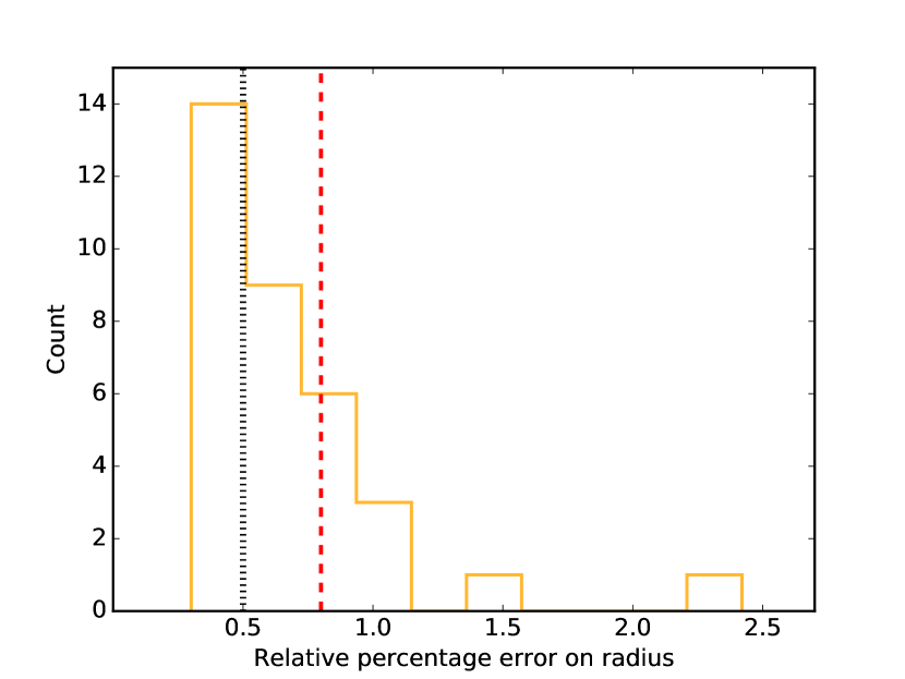
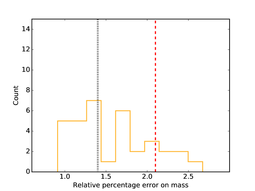
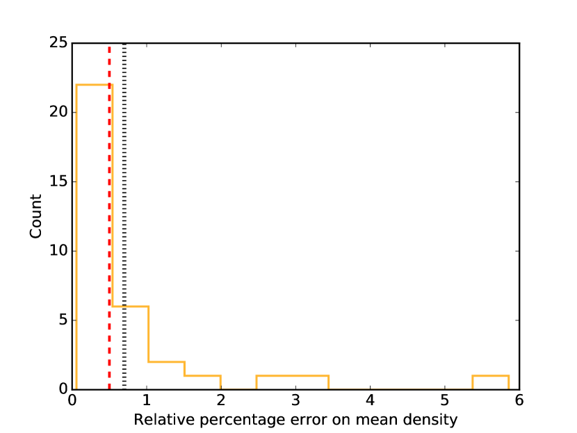
Figure 2: Statistical uncertainties and internal systematics. Histograms represent the distributions of statistical uncertainties when adopting the reference grid GS98sta. Black dotted lines represent internal systematic contributions from AGS09 (composition). Red dashed lines represent internal systematic contributions from GS98nod (diffusion).

4.1 Diffusion

Atomic diffusion (or element diffusion) is a transport process that occurs in radiative regions of stars. It can be driven by temperature gradients (thermal diffusion), gravity or pressure gradients (gravitational settling), and composition gradients (chemical diffusion). Thermal diffusion and gravitational settling concentrate heavier elements towards the centre of the star (Thoul et al., 1994). These two processes are opposed by composition gradients. Atomic diffusion is a less efficient process in convective regions since convection is a highly vigorous process that occurs on shorter timescales. Diffusion requires a quiet environment so that settling is not prevented by large-scale motions (Chaboyer et al., 2001). We switch on element diffusion in MESA, which includes chemical diffusion and gravitational settling (Paxton et al., 2011). MESA’s diffusion module uses diffusion coefficients from Thoul et al. (1994) in order to solve Burger’s equations when calculating particle diffusion and gravitational settling.

Figure 3 (left panel) shows that stellar ages derived using GS98nod are systematically larger than those derived using GS98sta.

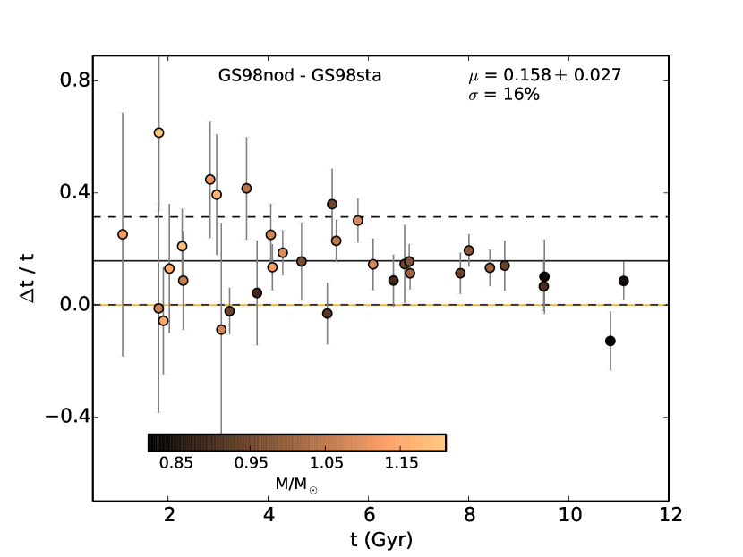
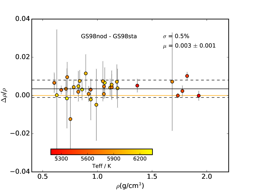
Figure 3: Fractional difference in age (left) and mean density (right) as a function of GS98sta stellar parameters. The colour-coding is with respect to stellar mass and effective temperature for the left and right panel, respectively. The solid black line indicates the bias ($\mu$), while the scatter ($\sigma$) is represented by the dashed lines. The zero level is represented by the solid orange line.

In our optimization process, we use the effective temperature and metallicity as classical observables. Since element diffusion changes surface element abundances, our GS98sta grid will need to have best fitting models with higher initial metal mass fractions so that the surface metal mass fractions can be comparable to the observed values at the stars’ current ages. This implies the opacity in the cores of these models will be higher throughout their evolution, compared to the case of no diffusion. To avoid the associated decrease in luminosity, which is indirectly constrained by the effective temperature and seismic data, the best fit models need to have higher mass, justifying their younger age. This is confirmed in Fig. 4 (left panel) where we show the fractional differences in the stellar mass. In turn, the strong constraints on the mean density imposed by the seismic data lead to an increase in the radius of the best fit models in our GS98sta grid, as shown in Fig. 4 (right panel). In summary, in order to satisfy the observables, models with diffusion need to have higher masses, hence also higher radii and younger ages.

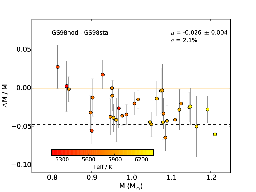
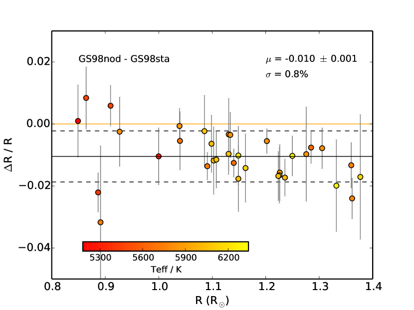
Figure 4: Fractional difference in mass (left) and radius (right) as a function of GS98sta stellar parameters. The zero level is represented by the solid orange line. The colour-coding is with respect to effective temperature. The solid black line indicates the bias ($\mu$), while the scatter ($\sigma$) is represented by the dashed lines.

We explore internal systematics by comparing models with and without diffusion, resulting in 0.5%, 0.8%, 2.1%, and 16% in mean density, radius, mass, and age, respectively (see Figs. 3 and 4). The internal systematics in density, mass, and radius are comparable to their statistical uncertainties, while the internal systematics in age are significantly larger than the statistical uncertainties (See Fig. 2).

Furthermore, we inspect the data presented in both Fig. 3 and Fig. 4 for the presence of linear correlations. We employ a correlation coefficient analysis developed in a Bayesian framework (Figueira et al., 2016). Using it we can estimate the posterior probability distribution of the correlation coefficient. Table 3 shows the results from such Bayesian test. At the 95% confidence level, there is a negative linear trend present for the radius and mass, with a hint of a similar trend being present for the age.

Table 3: Statistical summary of the posterior probability distribution of the correlation coefficient. C.I. denotes the confidence interval.

Parameter	Mean	Standard Deviation	95% C.I.
Mass	-0.433	0.135	[-0.69, -0.168]
Radius	-0.342	0.142	[-0.599, -0.049]
Age	-0.247	0.152	[-0.535, 0.047]

The difference between the initial and current metal mass fraction, $Z$, of the best-fitting models of GS98sta increases with increasing stellar mass. This suggests that gravitational settling has a larger impact on higher mass stars, explaining the trend with mass seen in Fig. 4.

4.2 Composition

Solar metallicity mixtures are one of the most important ingredients in stellar modelling. Here we focus on the most commonly used solar metallicity mixtures in constructing standard solar models, namely, those from Grevesse & Sauval (1998) and Asplund et al. (2009). We define [Fe/H] in all our calculations as

$$\mbox{[Fe/H]}=\log\left(\frac{Z_{\rm surface}}{X_{\rm surface}}\right)_{\rm star}-~{}\log\left(\frac{Z_{\rm surface}}{X_{\rm surface}}\right)_{\odot}~{}~{}~{},$$ (6)

where $X_{\rm surface}$ and $Z_{\rm surface}$ refer to the surface hydrogen and heavy element mass fractions, respectively. We used solar $Z_{\rm surface}$ values of 0.0134 and 0.0169 based on Asplund et al. and Grevesse & Sauval, respectively. In general, the solar metallicity mixture from AGS09 are lower than those from GS98sta. Basu & Antia (2004) demonstrate that the uncertainty in solar metallicity mixture result in differences in the sound speed in the stellar interiors.

We assess the internal systematics arising from the uncertainty in solar metallicity mixture.

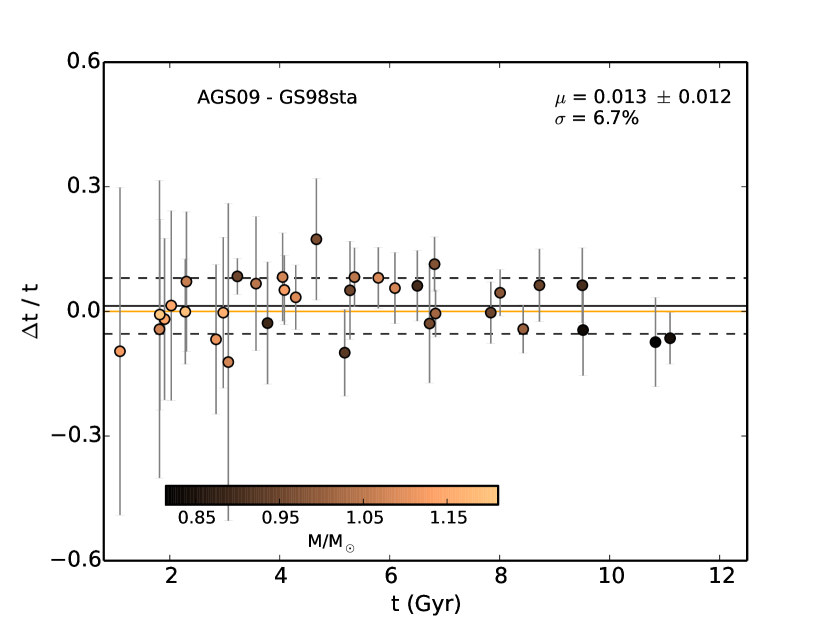
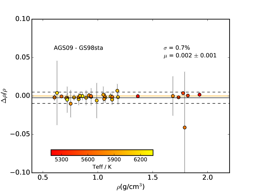
Figure 5: Fractional difference in age (left) and mean density (right) as a function of GS98sta stellar parameters. The colour-coding is with respect to stellar mass. The zero level is represented by the solid orange line. The solid black line indicates the bias ($\mu$), while the scatter ($\sigma$) is represented by the dashed lines.

We find a good agreement in both the derived ages and densities with internal systematics of 6.7% (with a bias of 0.013 $\pm$ 0.012) and 0.7% (with a bias of 0.002 $\pm$ 0.001), respectively (see Fig. 5). Internal systematics in stellar ages are somewhat smaller than the statistical uncertainties (median of 7.4%) as shown in Fig. 2. Furthermore, we find internal systematics of 0.5% in radius and 1.4% in mass (see Fig. 6).

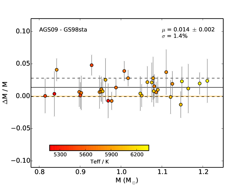
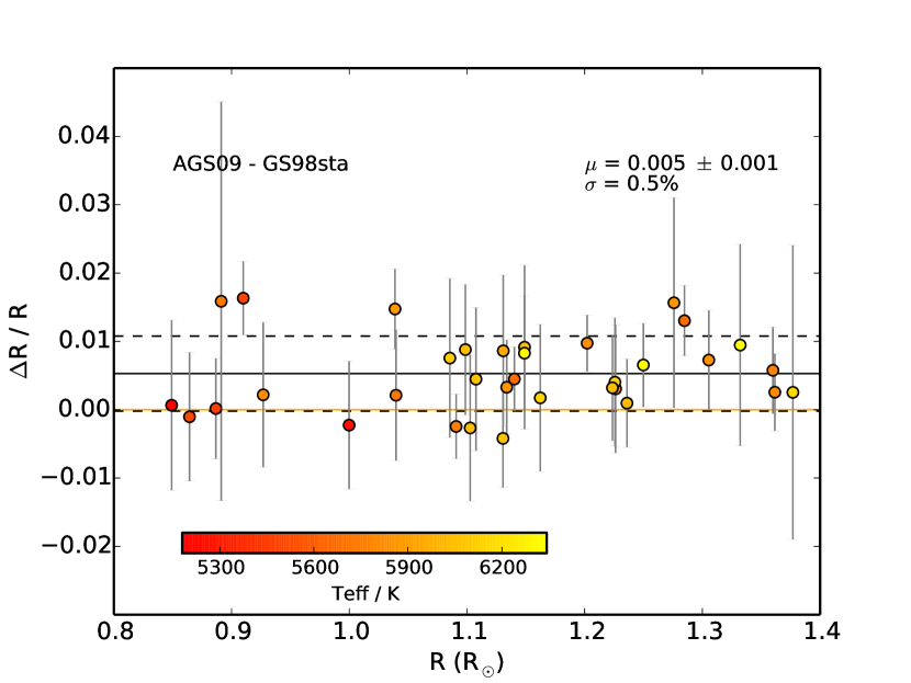
Figure 6: Fractional difference in mass (left) and radius (right) as a function of GS98sta stellar parameters. The zero level is represented by the solid orange line. The colour-coding is with respect to effective temperature. The solid black line indicates the bias ($\mu$), while the scatter ($\sigma$) is represented by the dashed lines.

Silva Aguirre et al. (2015) found systematic contributions arising from the uncertainty in solar metallicity mixture to be 0.3% in mean density and radius, 0.6% in mass and 3.3% in age. The internal systematics found in this work are approximately twice as large as those found by Silva Aguirre et al. (2015). The most probable cause for this discrepancy is in the treatment of the mixing length parameter ($\alpha_{\rm mlt}$). In this paper, we set $\alpha_{\rm mlt}$ as a free variable in all of our grids (see Sect. 3.1), while Silva Aguirre et al. (2015) used solar calibrated $\alpha_{\rm mlt}$ values. We note that the uncertainty in solar metallicity mixture will cause variations in solar calibrated values of $\alpha_{\rm mlt}$. Systematic uncertainties arising from grids varying in the treatment of $\alpha_{\rm mlt}$ were found to be 0.7%, 0.6%, 2.2%, and 9.0% in mean density, radius, mass, and age, respectively (Silva Aguirre et al., 2015). In addition, based on a grid of 3D convection simulations, $\alpha_{\rm mlt}$ has been shown to span a range of values on the main-sequence (Trampedach et al., 2014). It is therefore advisable to use a range of $\alpha_{\rm mlt}$ values when constructing stellar grids for Sun-like stars.

4.3 Surface correction

To overcome the well-known systematic differences between model and observed oscillation frequencies (Sect. 3), several surface correction methods have been put forward (see Table 4). The function, $f$, used in the different surface correction methods is given by

$$f=\frac{\nu}{\nu_{0}}~{}~{},$$ (7)

where $\nu$ is the mode oscillation frequency and $\nu_{0}$ a reference frequency. When using surface correction method proposed by Sonoi et al. (2015), the value of $\nu_{0}$ is determined in AIMS by means of the scaling relation (Brown et al., 1991; Kjeldsen & Bedding, 1995):

$$\nu_{0}=\left(\frac{M}{\mbox{M}_{\odot}}\right)\left(\frac{R}{\mbox{R}_{\odot}}\right)^{-2}\left(\frac{T_{\rm eff}}{T_{{\rm eff},\odot}}\right)^{-1/2}\nu_{{\rm max},\odot}~{}~{}.$$ (8)

The adopted solar values are $\nu_{{\rm max},\odot}=3104.0\>{\rm\mu Hz}$, ${\rm R}_{\odot}=6.9599\times 10^{10}\>{\rm cm}$, ${\rm M}_{\odot}=1.98919\times 10^{33}\>{\rm g}$, and $T_{\rm eff,\odot}=5777.0\>{\rm K}$ (Allen, 1976; Mamajek, 2012; Mosser et al., 2013).

Table 4: Summary of the different surface correction methods. $a$ and $b$ are best-fit parameters (see text for details), $f$ is a function that depends on the mode frequency, $I$ is the normalised mode inertia, and $\delta\nu$ is the offset between observed and model frequencies.

Name	Functions	b - value	Reference
KJ	$\delta\nu=af^{b}$	4.9	Kjeldsen et al. (2008)
BG1	$\delta\nu=af^{3}/I$	-	Ball & Gizon (2014)
BG2	$\delta\nu=(af^{-1}+bf^{3})/I$	-	Ball & Gizon (2014)
Sonoi	$\delta\nu=a\left(1-\frac{1}{1+f^{b}}\right)$	4.0	Sonoi et al. (2015)

For other surface corrections, we used

$$\nu_{0}=\frac{1}{2\pi}~{}\sqrt[]{\frac{GM}{R}}~{}~{},$$ (9)

where $G$ and $R$ are the gravitational constant and model radius, respectively. This does not make a difference on the correction, but only affects the magnitude of the fitting coefficients (i.e., $a$ and $b$). Some striking differences between the different surface correction methods are worth mentioning. Kjeldsen et al. (2008) proposed that the offset depends on a power of the mode frequency, whose exponent, $b$, they determined to be $b=4.9$ (calibrated with respect to solar data). The same value has subsequently been adopted in the study of other stars (Metcalfe et al., 2010; Brandão et al., 2011; Van Eylen et al., 2012; Gruberbauer et al., 2013). Using Canuto-Goldman-Mazzitelli (CGM) modelling of convection, Deheuvels et al. (2014) determined a value of $b$ to be $4.25$ and adopted it in generating models using the Cesam2k evolutionary code. We adopted the former value of $b$ in AIMS when using the surface correction of Kjeldsen et al. (2008), as shown in Table 4. Sonoi et al. (2015) established that the power-law function proposed by Kjeldsen et al. (2008) is not satisfactory in fitting the high-frequency range. This was attributed to the nature of the profile of the frequency difference, $\delta\nu$, which becomes less steep as the frequency increases beyond $\nu_{\rm max}$. Sonoi et al. (2015) thus proposed a Lorentzian function that they found to better fit the profile of the frequency difference across the whole frequency range. It should be noted that the modified Lorentzian function proposed by Sonoi et al. (2015) reduces to the equation proposed by Kjeldsen et al. (2008) when $f\ll 1$. Furthermore, the scaling factor, $r$, related to the mean density and proposed by Kjeldsen et al. (2008), is not used in AIMS. The risk with rescaling the model is that one will need to change a number of variables (e.g. how is heat transport affected). It may be possible to rescale the acoustic variables consistently, but other variables may not remain consistent. Hence, for this reason the $r$-scaling is not implemented in AIMS. If there is a mismatch, then AIMS looks for another model where the mean density is closer, rather than trying to rescale the model to the right mean density. Ball & Gizon (2014) proposed two functions (BG1 and BG2, see Table 4), both taking into account the mode inertia, $I$. This was based on findings of Gough (1990) and Goldreich et al. (1991) who argued that perturbations caused by a magnetic field would cause changes proportional to $\nu^{3}/I$ and a change in the description of convection is expected to cause changes proportional to $\nu^{-1}/I$. BG1 takes into account only the cubic term while BG2 combines both terms (see Table 4).
We note that we used the same set of observed frequencies for each star when applying the different surface correction methods during the optimisation process. This is because we aimed at carrying out a uniform analysis for all the different surface correction methods.

We explore the internal systematics from adopting the different surface correction options by comparing the model parameters derived in each case with those obtained when using frequency ratios. Frequency ratios have been shown to be less affected by the poorly modelled surface layers and this permits direct comparison of observed oscillation frequencies with the theoretical oscillations frequencies without applying any surface correction routine (Roxburgh & Vorontsov 2003; Silva Aguirre et al. 2011; Silva Aguirre et al. 2015, 2017). Unfortunately, some information about the star is lost when one uses frequency ratios. For instance, since the stellar mean density scales with the frequencies, taking frequency ratios results into factoring out the mean density and thus making frequency ratios less sensitive to the mean density compared to direct comparison with oscillation frequencies (Roxburgh & Vorontsov, 2003). Despite this, frequency ratios have been reported to constrain stellar interiors, resulting in more precise asteroseismic stellar ages compared to the use of individual frequencies. In AIMS, we specified the frequency ratios $r_{10}$, $r_{01}$, and $r_{02}$ as (Roxburgh & Vorontsov, 2003):

$$r_{01}(n)=\frac{d_{01}(n)}{\Delta\nu_{1}(n)}~{},~{}~{}~{}r_{10}(n)=\frac{d_{10}(n)}{\Delta\nu_{0}(n+1)}~{}~{},$$ (10)

$$r_{02}(n)=\frac{d_{02}(n)}{\Delta\nu_{1}(n)}~{},$$ (11)

where $\Delta\nu_{l}(n)=\nu_{n,l}-\nu_{n-1,l}$ is the large frequency separation, $n$ is the mode radial order, $l$ is the mode harmonic degree, and $d_{02}(n)=\nu_{n,0}-\nu_{n-1,2}$ is the small frequency separation. Moreover, $d_{01}(n)$ and $d_{10}(n)$ are defined as:

$$d_{01}(n)=\frac{1}{8}(\nu_{n-1,0}-4\nu_{n-1,1}+6\nu_{n,0}-4\nu_{n,1}+\nu_{n+1,0})~{}~{},$$ (12)

$$d_{10}(n)=-\frac{1}{8}(\nu_{n-1,1}-4\nu_{n,0}+6\nu_{n,1}-4\nu_{n+1,0}+\nu_{n+1,1})~{}~{}.$$ (13)

Hereafter, the surface correction method by Kjeldsen et al. (2008) is denoted by KJ, Sonoi et al. (2015) as Sonoi, Ball & Gizon (2014) one-term correction as BG1, and Ball & Gizon (2014) two-term correction as BG2 (See Table 4). Sonoi and BG2 lead to smaller internal systematics in mass: 2.0% and 1.7%, respectively (see Fig. 7). We find that the masses are overestimated when employing the corrections by KJ and BG1. KJ also yields internal systematics of 2.0% in mass, albeit affected by a larger bias of 0.029 $\pm$ 0.004. All surface correction routines yield similar internal systematics in radius, with BG1 leading to the largest bias (see Fig. 8). Both KJ and BG2 produce internal systematics in radius of 0.8%, while Sonoi yields 0.9%.

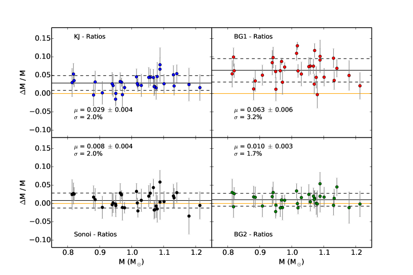
Figure 7: Fractional difference in mass as a function of GS98sta stellar masses. The zero level is represented by the solid orange line. The solid black line indicates the bias ($\mu$), while the scatter ($\sigma$) is represented by the dashed lines.

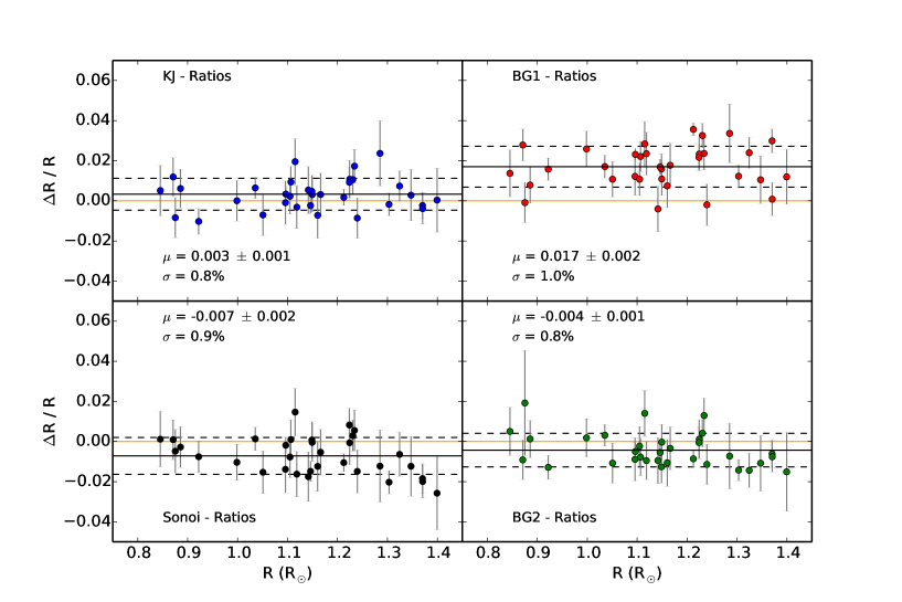
Figure 8: Fractional difference in radius as a function of GS98sta stellar radii. The solid black line indicates the bias ($\mu$), while the scatter ($\sigma$) is represented by the dashed lines. The zero level is represented by the solid orange line.

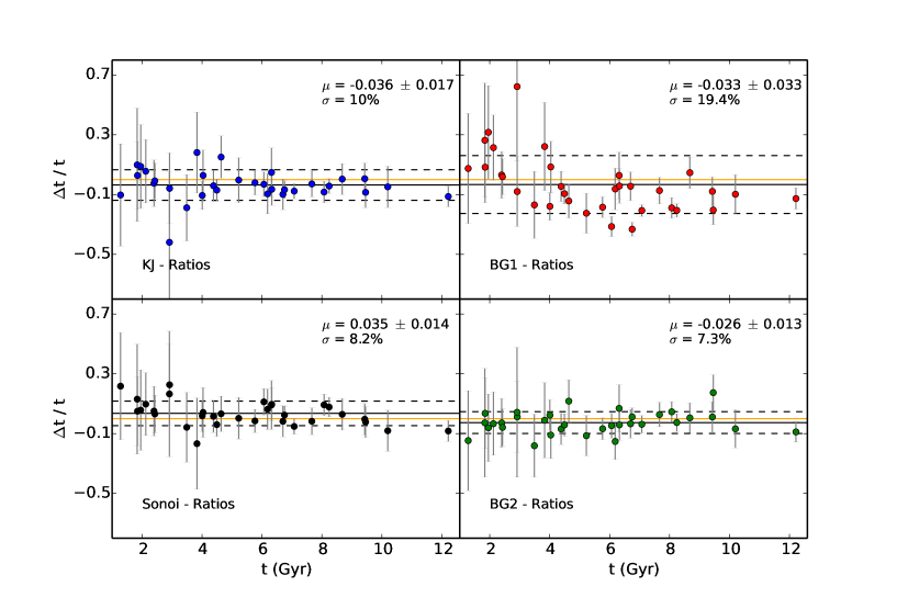
Figure 9: Fractional difference in age as a function of GS98sta stellar ages. The zero level is represented by the solid orange line. The solid black line indicates the bias ($\mu$), while the scatter ($\sigma$) is represented by the dashed lines.

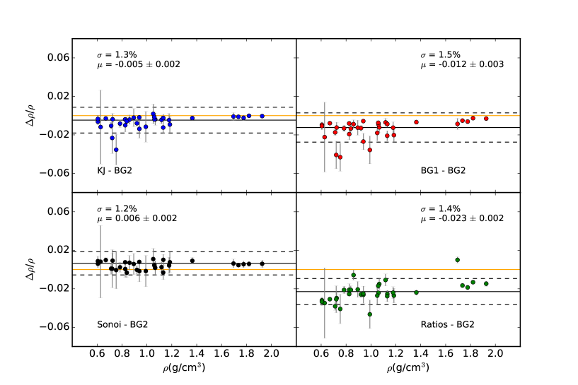
Figure 10: Fractional difference in stellar mean density as a function of GS98sta stellar mean density. The zero level is represented by the solid orange line. The solid black line indicates the bias ($\mu$), while the scatter ($\sigma$) is represented by the dashed lines.

Figure 9 shows that Sonoi and BG2 produce smaller internal systematics in age: 8.2% and 7.2%, respectively. KJ results in internal systematics of 10%, while BG1 yields the largest internal systematics (19.4%).

BG2 yields the least median reduced $\chi^{2}_{\nu}$ in the model-to-observed frequency differences of 5.661. Sonoi and KJ yield comparable median reduced $\chi^{2}_{\nu}$ of 15.846 and 15.958, respectively. BG1 gives median reduced $\chi^{2}_{\nu}$ of 27.800. This in turn explains why the BG2 lead to the least internal systematics followed by Sonoi.

In Fig. 10, we consider BG2 results as the reference in the comparison with the different surface correction methods. This is because from Figs. 7, 8, and 9, BG2 yields the least internal systematics in mass, radius, and age, respectively. In addition, frequency ratios will provide a poor description of the near-surface layers. It can clearly be seen in Fig. 10 that some information about the mean density is lost when one uses frequency ratios. Since we used uncorrected model frequencies to compute the frequency ratios as well as the large frequency separation, the later includes a significant contribution from the surface effect. Assuming that the large frequency separation for the best fitting model matched reasonably well with the observed separation, the "true" large separation for the model (excluding the surface effect contribution) is significantly underestimated, and hence the corresponding mean density. This is consistent with previous findings by Silva Aguirre et al. (2017). The internal systematics on the mean density arising from varying the surface correction methods are found to be less than 1.5%.

We note that when one compares the observed frequencies with the uncorrected theoretical frequencies of the best-fit models obtained using the different surface correction methods, surface corrections should be expected to tend to zero only for low enough frequencies. This is because, assuming the shape of the surface correction does not match with the differences between the observed and “true model” frequencies, then the best fitting model obtained by minimizing the differences between the observed and surface corrected model frequencies would show differences at the low frequency end. This arises from how the model frequencies evolve as the model itself evolves. It turns out that if the shape of the assumed surface correction is not correct, then one ends up with either under or over evolved model as best fitting model (depending on whether assumed surface correction over corrects or under corrects). When only frequency ratios are used as seismic constraints, a much larger difference between the observed and uncorrected theoretical frequencies is obtained at the lower frequency end. This is expected since frequency ratios do not carry information about the surface layers. This has a stronger impact on the radius and density. It is for this reason we added the large separation calculated from $l=0$ mode frequencies.

5 Summary

We investigated the internal systematics in mean density, radius, mass, and age arising from changes in particular physical aspects of stellar models. We did so based on the analysis of stellar model grids constructed as uniformly as possible and only varying the input physics being considered. However, internal systematics arising from the uncertainty in solar metallicity mixture will contain contributions from their respective opacities. Moreover, we also assessed the internal systematics arising from the use of different surface correction methods in forward modelling.

We found internal systematics from the uncertainty in solar metallicity mixture to be comparable to the statistical uncertainties. Specifically, we found internal systematics of 0.7%, 0.5%, 1.4%, and 6.7% in mean density, radius, mass, and age, respectively. Relative median statistical uncertainties from using our reference grid (GS98sta) are 0.3% in density, 0.6% in radius, 1.6% in mass, and 7.4% in age. Silva Aguirre et al. (2015) found systematic contributions arising the uncertainty in solar metallicity mixture to be 0.3% in density and radius, 0.6% in mass and 3.3% in age. The internal systematics found in this work are approximately twice as large as those found by Silva Aguirre et al. (2015). The most probable cause for this difference is the fact that we treat the mixing length parameter, $\alpha_{\rm mlt}$ (see Sect. 4.2) as a free parameter.

Concerning the impact of diffusion, we have shown that the inclusion of diffusion in stellar grids of solar-type stars leads to models with significantly lower ages. This is consistent with previous findings (Silva Aguirre et al., 2015; Dotter et al., 2017). We found internal systematics of 0.5%, 0.8%, 2.1%, and 16% in mean density, radius, mass, and age, respectively. The internal systematics in age are significantly larger than the corresponding statistical uncertainties.

We assessed the impact of using different surface correction methods on the derived stellar parameters. We found the corrections by Sonoi and BG2 to yield the least internal systematics, namely, 0.9% and 0.8% in radius, 2.0% and 1.7% in mass, and 8.2% and 7.3% in age, respectively. These internal systematics are comparable to the statistical uncertainties. KJ performs satisfactorily for our sample (see discussion in Sect. 4.3), while BG1 yields the largest internal systematics as well as the largest biases for stellar radius and mass. We found stellar masses to be overestimated when using the KJ and BG1 corrections.

Asteroseismology is proving to be particularly significant for the study of solar-type stars, in great part due to the exquisite data that have been made available by NASA’s Kepler space telescope. The future looks even brighter, with NASA’s TESS and ESA’s PLATO space missions promising to revolutionise the field and increase the number of stars with detected oscillations by several orders of magnitude. The information contained in stellar oscillations allows the internal stellar structure to be constrained to unprecedented levels, while also allowing fundamental stellar properties (e.g. mass, radius, and age) to be precisely determined. In anticipation of the flood of observations from future space missions, a number of state-of-the-art asteroseismic techniques for the estimation of fundamental stellar properties are currently being developed and tested. Particular attention is being placed on calibrating the determination of age, due to the strong dependence this quantity has on stellar physics. This work therefore provides a valuable contribution to this communal effort by assessing the systematics on the derived stellar properties that arise from specific changes in the model input physics.

References

- Allen (1976) Allen C. W., 1976, Astrophysical Quantities
- Aller & Chapman (1960) Aller L. H., Chapman S., 1960, ApJ, 132, 461
- Angulo et al. (1999) Angulo C., et al., 1999, Nuclear Physics A, 656, 3
- Asplund et al. (2009) Asplund M., Grevesse N., Sauval A. J., Scott P., 2009, Annual Review of Astron and Astrophys, 47, 481
- Ball & Gizon (2014) Ball W. H., Gizon L., 2014, A & A, 568, A123
- Ball & Gizon (2017) Ball W. H., Gizon L., 2017, A & A, 600, A128
- Balser (2006) Balser D. S., 2006, Astronomical Journal, 132, 2326
- Basu & Antia (2004) Basu S., Antia H. M., 2004, ApJL, 606, L85
- Benomar et al. (2014) Benomar O., Masuda K., Shibahashi H., Suto Y., 2014, PASJ, 66, 94
- Böhm-Vitense (1958) Böhm-Vitense E., 1958, Zeit. Astrophys., 46, 108
- Borucki et al. (2010) Borucki W. J., et al., 2010, Science, 327, 977
- Brandão et al. (2011) Brandão I. M., et al., 2011, A & A, 527, A37
- Brown et al. (1991) Brown T. M., Gilliland R. L., Noyes R. W., Ramsey L. W., 1991, ApJ, 368, 599
- Campante et al. (2015) Campante T. L., et al., 2015, ApJ, 799, 170
- Campante et al. (2016a) Campante T. L., et al., 2016a, ApJ, 819, 85
- Campante et al. (2016b) Campante T. L., et al., 2016b, ApJ, 830, 138
- Campante et al. (2017) Campante T. L., Santos N. C., Monteiro M. J. P. F. G., 2017, preprint, (arXiv:1709.00645)
- Casagrande et al. (2007) Casagrande L., Flynn C., Portinari L., Girardi L., Jimenez R., 2007, MNRAS, 382, 1516
- Casagrande et al. (2014) Casagrande L., et al., 2014, ApJ, 787, 110
- Chaboyer et al. (2001) Chaboyer B., Fenton W. H., Nelan J. E., Patnaude D. J., Simon F. E., 2001, ApJ, 562, 521
- Chiosi & Matteucci (1982) Chiosi C., Matteucci F. M., 1982, A & A, 105, 140
- Christensen-Dalsgaard & Thompson (1997) Christensen-Dalsgaard J., Thompson M. J., 1997, MNRAS, 284, 527
- Christensen-Dalsgaard et al. (1988) Christensen-Dalsgaard J., Dappen W., Lebreton Y., 1988, Nature, 336, 634
- Christensen-Dalsgaard et al. (1993) Christensen-Dalsgaard J., Proffitt C. R., Thompson M. J., 1993, ApJ, 403, L75
- Christensen-Dalsgaard et al. (2011) Christensen-Dalsgaard J., Monteiro M. J. P. F. G., Rempel M., Thompson M. J., 2011, MNRAS, 414, 1158
- Cyburt et al. (2003) Cyburt R. H., Fields B. D., Olive K. A., 2003, Physics Letters B, 567, 227
- Davies et al. (2016) Davies G. R., et al., 2016, MNRAS, 456, 2183
- Deheuvels & Michel (2011) Deheuvels S., Michel E., 2011, A & A, 535, A91
- Deheuvels et al. (2014) Deheuvels S., et al., 2014, A & A, 564, A27
- Dotter et al. (2017) Dotter A., Conroy C., Cargile P., Asplund M., 2017, ApJ, 840, 99
- Dziembowski et al. (1988) Dziembowski W. A., Paterno L., Ventura R., 1988, A & A, 200, 213
- Ferguson et al. (2005) Ferguson J. W., Alexander D. R., Allard F., Barman T., Bodnarik J. G., Hauschildt P. H., Heffner-Wong A., Tamanai A., 2005, ApJ, 623, 585
- Figueira et al. (2016) Figueira P., Faria J. P., Adibekyan V. Z., Oshagh M., Santos N. C., 2016, Origins of Life and Evolution of the Biosphere, 46, 385
- Foreman-Mackey et al. (2013) Foreman-Mackey D., Hogg D. W., Lang D., Goodman J., 2013, PASP, 125, 306
- Goldreich et al. (1991) Goldreich P., Murray N., Willette G., Kumar P., 1991, ApJ, 370, 752
- Gough (1990) Gough D., 1990, Comments on helioseismic inference, in Progress of Seismology of the Sun and Stars. Springer Berlin Heidelberg, pp Lecture Notes in Physics, Vol 367, 283, doi:10.1007/3-540-53091-6_93
- Gregory (2005) Gregory P. C., 2005, Bayesian Logical Data Analysis for the Physical Sciences: A Comparative Approach with ‘Mathematica’ Support. Cambridge University Press
- Grevesse & Sauval (1998) Grevesse N., Sauval A. J., 1998, Space Science Reviews, 85, 161
- Gruberbauer et al. (2013) Gruberbauer M., Guenther D. B., MacLeod K., Kallinger T., 2013, MNRAS, 435, 242
- Guzik & Cox (1993) Guzik J. A., Cox A. N., 1993, ApJ, 411, 394
- Huber et al. (2013) Huber D., et al., 2013, ApJ, 767, 127
- Iglesias & Rogers (1996) Iglesias C. A., Rogers F. J., 1996, ApJ, 464, 943
- Imbriani et al. (2005) Imbriani G., et al., 2005, EPJ A, 25, 455
- Jimenez et al. (2003) Jimenez R., Flynn C., MacDonald J., Gibson B. K., 2003, Science, 299, 1552
- Kjeldsen & Bedding (1995) Kjeldsen H., Bedding T. R., 1995, A&A, 293, 87
- Kjeldsen et al. (2008) Kjeldsen H., Bedding T. R., Christensen-Dalsgaard J., 2008, ApJL, 683, L175
- Korn et al. (2007) Korn A. J., Grundahl F., Richard O., Mashonkina L., Barklem P. S., Collet R., Gustafsson B., Piskunov N., 2007, ApJ, 671, 402
- Kunz et al. (2002) Kunz R., Fey M., Jaeger M., Mayer A., Hammer J. W., Staudt G., Harissopulos S., Paradellis T., 2002, ApJ, 567, 643
- Lebreton & Goupil (2014) Lebreton Y., Goupil M. J., 2014, A & A, 569, A21
- Lodders & Palme (2009) Lodders K., Palme H., 2009, Meteoritics and Planetary Science Supplement, 72, 5154
- Lund et al. (2017) Lund M. N., et al., 2017, ApJ, 835, 172
- Maeder & Meynet (2000) Maeder A., Meynet G., 2000, Annual Review of Astron and Astrophys, 38, 143
- Mamajek (2012) Mamajek E. E., 2012, ApJL, 754, L20
- Marcy et al. (2014) Marcy G. W., et al., 2014, ApJS, 210, 20
- Mathur et al. (2012) Mathur S., et al., 2012, ApJ, 749, 152
- Metcalfe et al. (2010) Metcalfe T. S., et al., 2010, ApJ, 723, 1583
- Metcalfe et al. (2012) Metcalfe T. S., et al., 2012, APJL, 748, L10
- Metcalfe et al. (2014) Metcalfe T. S., et al., 2014, ApJS, 214, 27
- Miglio & Montalbán (2005) Miglio A., Montalbán J., 2005, A&A, 441, 615
- Monteiro et al. (1996) Monteiro M. J. P. F. G., Christensen-Dalsgaard J., Thompson M. J., 1996, A & A, 307, 624
- Mosser et al. (2013) Mosser B., et al., 2013, A&A, 550, A126
- Nsamba et al. (2017) Nsamba B., Monteiro M. J. P. F. G., Campante T. L., Reese D. R., White T. R., García Hernández A., Jiang C., 2017, EPJ Web Conf., 160, 05010
- Paxton et al. (2011) Paxton B., Bildsten L., Dotter A., Herwig F., Lesaffre P., Timmes F., 2011, ApJS, 192, 3
- Paxton et al. (2013) Paxton B., et al., 2013, ApJS, 208, 4
- Paxton et al. (2015) Paxton B., et al., 2015, ApJS, 220, 15
- Perryman (2014) Perryman M., 2014, The Exoplanet Handbook, Cambridge, UK: Cambridge University Press
- Piau et al. (2011) Piau L., Kervella P., Dib S., Hauschildt P., 2011, A & A, 526, A100
- Pinsonneault et al. (2012) Pinsonneault M. H., An D., Molenda-Żakowicz J., Chaplin W. J., Metcalfe T. S., Bruntt H., 2012, ApJS, 199, 30
- Pinsonneault et al. (2014) Pinsonneault M. H., et al., 2014, ApJS, 215, 19
- Ramírez et al. (2009) Ramírez I., Meléndez J., Asplund M., 2009, A & A, 508, L17
- Rauer et al. (2014) Rauer H., et al., 2014, Experimental Astronomy, 38, 249
- Rogers & Nayfonov (2002) Rogers F. J., Nayfonov A., 2002, ApJ, 576, 1064
- Roxburgh & Vorontsov (2003) Roxburgh I. W., Vorontsov S. V., 2003, A & A, 411, 215
- Serenelli & Basu (2010) Serenelli A. M., Basu S., 2010, ApJ, 719, 865
- Silva Aguirre et al. (2011) Silva Aguirre V., Ballot J., Serenelli A. M., Weiss A., 2011, A & A, 529, A63
- Silva Aguirre et al. (2013) Silva Aguirre V., et al., 2013, ApJ, 769, 141