Distributed Load-Side Control: Coping with Variation of Renewable Generations

Abstract

This paper addresses the distributed frequency control problem in a multi-area power system taking into account of unknown time-varying power imbalance. Particularly, fast controllable loads are utilized to restore system frequency under changing power imbalance in an optimal manner. The imbalanced power causing frequency deviation is decomposed into three parts: a known constant part, an unknown low-frequency variation and a high-frequency residual. The known steady part is usually the prediction of power imbalance. The variation may result from the fluctuation of renewable resources, electric vehicle charging, etc., which is usually unknown to operators. The high-frequency residual is usually unknown and treated as an external disturbance. Correspondingly, in this paper, we resolve the following three problems in different timescales: 1) allocate the steady part of power imbalance economically; 2) mitigate the effect of unknown low-frequency power variation locally; 3) attenuate unknown high-frequency disturbances. To this end, a distributed controller combining consensus method with adaptive internal model control is proposed. We first prove that the closed-loop system is asymptotically stable and converges to the optimal solution of an optimization problem if the external disturbance is not included. We then prove that the power variation can be mitigated accurately. Furthermore, we show that the closed-loop system is robust against both parameter uncertainty and external disturbances. The New England system is used to verify the efficacy of our design.

1 Introduction

1.1 Background

In the modern power system, multiple regional grids are usually interconnected to constitute a bulk grid Min and Abur (2006); Ahmadi-Khatir et al. (2013). To maintain a stable power system, the frequency should be retained at its nominal value, e.g. 50Hz or 60Hz. Conventionally, it is realized by synchronized generators in a centralized fashion, known as a hierarchy control architecture Kundur (1994); Dörfler et al. (2016). However, with the increasing penetration of volatile and uncertain renewable generations, power mismatch in the system can fluctuate rapidly with a large amount. In such a situation, the traditional manner of control may not be able to keep pace due to large inertia of the traditional synchronous generators. Fortunately, load-side participation in frequency control opens up new possibility to resolve this problem, benefiting from its fast response Schweppe et al. (1980); Zhao et al. (2014). On the other hand, as controllable loads are usually dispersed across the power system, a distributed architecture is more suitable for load-side control than the conventional centralized one. Indeed, distributed optimal control has been investigated by combining controller design with optimal dispatch problems Jokić et al. (2009); Zhang and Papachristodoulou (2015); Stegink et al. (2017). It leads to a so-called reverse engineering methodology for designing optimal controllers, particularly in optimal frequency control of power systems Li et al. (2016); Zhao et al. (2014); Cai et al. (2017). In this paper, we design a distributed load-side controller that is capable of adapting to power variation due to volatile renewable generations, such as wind farms and PV clusters.

1.2 Related Work

In power system operation, frequency deviation is usually a consequence of power mismatch due to unexpected disturbances, such as sudden load leaping/dropping or generator tripping. Frequency control papers can be roughly divided into two categories in terms of the forms of power imbalance: constant power imbalance Zhao et al. (2014); Mallada et al. (2017); Wang et al. (2018); Kasis et al. (2017); Wang et al. (2017b, c); Lu et al. (2016) and time-varying power imbalance Trip et al. (2016); Xi et al. (2017); Weitenberg et al. (2017). In the first category, a step change of load/generation is considered. Then generators and/or controllable loads are utilized to eliminate the power imbalance and restore the nominal frequency. In Zhao et al. (2014), an optimal load-side control problem is formulated and a primary frequency controller is derived to balance step power change using controllable loads. It is extended in Mallada et al. (2017) to realize a secondary frequency control, i.e. restoring the nominal frequency. The design approach is generalized in Kasis et al. (2017), where the model requirement is relaxed and a passivity condition is proposed to guarantee asymptotic stability. Wang et al. (2017b, c) further consider both steady-state and transient operational constraints in distributed optimal frequency control. In Wang et al. (2018), a nonlinear network-preserving model is considered and only limited control coverage is needed to implement the distributed optimal frequency control. A different disturbance is considered in Lu et al. (2016), where the secondary frequency controller is injected by constant malicious attacks. To eliminate the influence of the attacks, a detection method is derived to combine with the distributed frequency controller.

In the second category, power imbalance is not constant, creating much greater challenge to controller design and stability analysis. In Trip et al. (2016), power variation is modeled as output of a known exosystem. Then an internal model controller is designed to tackle and compensate for the time-varying imbalanced power. The idea of combining distributed control with internal model control is attractive and inspiring. In Xi et al. (2017), a centralized controller is proposed, which can track the power imbalance and maintain the system frequency within a desired range in the presence slowly changing power imbalance. The frequency still varies along with time-varying loads. In Weitenberg et al. (2017), measurement noise is considered in frequency control, and a leaky integral controller is proposed that can strike an acceptable trade-off between performance and robustness.

To sum up, in most of the existing literature, power disturbance is modeled as a step change. The time-varying power disturbance is usually regarded as output of a known exosystem. However, neither model is realistic for practical power systems, especially when a large amount of renewable generations and electric vehicles are integrated. In such a situation, power imbalance is always time-varying and unknown, which should be carefully considered in the design of distributed frequency control.

1.3 Contribution

In this paper, power imbalance is decomposed into a known constant part, an unknown low-frequency time-varying part and a high-frequency residual. In power systems, the first one can be obtained by prediction while the latter two are fluctuations around the prediction. Offset error in prediction can also be considered in the unknown time-varying part. This decomposition suggests a way to deal with time-varying disturbances. First, a distributed control is proposed based on consensus method to balance the known constant part economically, which resolves a slow timescale operation problem. Second, a decentralized supplementary controller based on the internal model control is proposed to mitigate the effect of the unknown low-frequency variation at a faster timescale. Finally, we also ensure that the proposed controller attenuate the impact of high-frequency residual.

This work can be regarded as an extension of Zhao et al. (2014); Mallada et al. (2017); Wang et al. (2018); Kasis et al. (2017); Wang et al. (2017b, c). As the power imbalance is time varying in our case, these previous distributed controller may not be able to stabilize and restore the frequency, as we will demonstrate later in case studies. Here the main challenge is how to fit a time-varying tracking and compensation control into the structure of the previous distributed frequency controller. The major difference between this paper and Trip et al. (2016) is that the power variation is modeled as output of a known exosystem in Trip et al. (2016). Since such information is difficult to obtain in practice, our model appears to be more practical. In Wang et al. (2017a), an internal model control is leveraged to devise a distributed unconstrained optimization which can mitigate the effects of unknown time-varying disturbances. In contrast, we consider optimal frequency control problem with both power system dynamics as well as power balance constraints, which are not included in Wang et al. (2017a). Moreover, we also analyze the robustness of the proposed controller under uncertain parameters and disturbances. Main contributions of this paper are as follows:

• A generic model of power imbalance for frequency control is established, consisting of three parts: a known constant part, an unknown low-frequency power variation and a high-frequency residual. The power variation is further modeled by a superposition of several dominant sinusoidal components. Then it is formulated as the output of an exosystem with unknown parameters;

• A distributed controller is derived to restore the nominal frequency even under unknown disturbance. It is composed of two parts. One is designed based on consensus control to achieve an economic allocation of the constant part of power imbalance, while the other is designed based on adaptive internal model control to mitigate the effect of unknown power variation;

• Robustness of the controller under parameter uncertainty and external disturbances is analyzed. It is proved that the uncertain damping constant has no impact on the performance of the controller and the impact of external disturbances is attenuated greatly.

1.4 Organization

The rest of this paper is organized as follows. In Section 2, the network and power imbalance models are formulated. Section 3 presents the design of distributed frequency controller. In Section 4, the equilibrium of the closed-loop system is characterized with a proof of asymptotic stability. The robustness of the proposed controller under uncertainties is analyzed in Section 5. We confirm controller performance via simulations in Section 6. Section 7 concludes the paper.

2 Problem Formulation

2.1 Model of Power Network

A large power network is usually composed of multiple control areas, which are interconnected through tie lines. For simplicity, we treat each control area as a node with an aggregate controllable load and an aggregate uncontrollable power injection. Then the power network is modeled as a graph ${\cal G}:=(N,E)$ where $N=\{1,2,...n\}$ is the set of nodes (control areas) and $E\subseteq N\times N$ is the set of edges (tie lines). If a pair of nodes $i$ and $j$ are connected by a tie line directly, we denote the tie line by $(i,j)\in E$. $\cal G$ is treated as directed with an arbitrary orientation and we use $(i,j)\in E$ or $i\rightarrow j$ interchangeably to denote a directed edge from $i$ to $j$. Without loss of generality, we assume ${\cal G}$ is connected.

Besides the graph of physical power network, we also need to consider the communication network, modeled by a graph ${\cal H}$ whose nodes are the same set $N$ of graph ${\cal G}$ with possibly a different set of edges. An edge in ${\cal H}$ means that the two endpoints of the edge can communicate with each other directly. In this paper, we assume ${\cal H}$ is also connected. The set of neighbors of node $j$ in the communication graph ${\cal H}$ is denoted by $N_{cj}$. The Laplacian matrix of ${\cal H}$ is denoted as $L$.

A second-order linearized model is adopted to describe the frequency dynamics of each node. We assume the tie lines are lossless and adopt the DC power flow model, which is reasonable for a high-voltage transmission system. Then for each node $j\in N$, we have

$$\dot{\theta}_{j}\ =\ \omega_{j}$$ (1a)

$$M_{j}\dot{\omega}_{j}\ =\ P^{in}_{j}-P^{l}_{j}-D_{j}\omega_{j}$$

$$\quad+\sum\nolimits_{i:i\rightarrow j}\!B_{ij}(\theta_{i}-\theta_{j})-\sum\nolimits_{k:j\rightarrow k}\!B_{jk}(\theta_{j}-\theta_{k})$$ (1b)

where, $\theta_{j}$ denotes the rotor angle at node $j$; $\omega_{j}$ the frequency deviation; $P^{in}_{j}$ the uncontrollable power injection; $P^{l}_{j}$ the controllable load. $M_{j}>0,\ D_{j}>0$ are inertia and damping constants, respectively. $B_{jk}>0$ are line parameters that depend on the reactances of line $(j,k)\in E$.

2.2 Model of Power Imbalance

Denote $P^{in}_{j}$ as the imbalanced power in the system. It can be decomposed into two parts: a constant part and a variation part. That is

$$P_{j}^{in}(t)=\overline{P}_{j}^{in}+\tilde{q}_{j}(t)$$ (2)

where $\overline{P}_{j}^{in}$ is the known constant part, which could be the prediction of renewable generations and/or loads. $\tilde{q}_{j}(t)$ is the variation part, which is assumed unknown.

The known constant part is easy to deal with, while the variation part is non-trivial. The main idea is to further decompose it into the sum of a series of sinusoidal functions, whose parameters are unknown. Then an internal model control can be utilized to trace these sinusoidal components, and then eliminate the effects of the variation part.

In light of Milan et al. (2013); Bušiā and Meyn (2016); Barooah et al. (2015); Aguirre et al. (2008), we can approximate variation of renewable generations and load demands by a superposition of a few sinusoidal functions. Specifically, we decompose the power imbalance $\tilde{q}_{j}(t)$ at node $j$ injected by volatile renewable generation and loads into

$$\tilde{q}_{j}(t):=q_{j0}+\sum\nolimits_{k=1}^{s_{j}}q_{jk}\sin(a_{jk}\cdot t+\phi_{jk})+w_{j}(t)$$ (3)

where $q_{j0}$ is the prediction offset error (which is an unknown constant). The second term models the variation part, which is a superposition of $s_{j}$ sinusoidal functions. Their amplitudes $q_{jk}$, frequencies $a_{jk}>0$ and initial phases $\phi_{jk}$ are unknown but belong to a known bounded interval. Here we consider only a few low-frequency power fluctuations. The remaining high-frequency residuals, denoted by $w_{j}(t)$, is usually quite small. So we treat $w_{j}(t)$ as an external disturbance and do not consider its detailed model in this paper, but simply assume that it belongs to the $\mathcal{L}_{2}^{T}$ space, i.e., for any $w_{j}(t)\;\;(j\in N)$, $\int_{0}^{T}||w_{j}(t)||^{2}\text{d}t<+\infty$ holds for all $0<T<+\infty$.

Remark 1 (Power Variation in power system).

In this paper, we adopt a generic model to depict $\tilde{q}_{j}(t)$ so that it is applicable to various types of power imbalance in practice. In practical power systems, $\tilde{q}_{j}(t)$ has many interpretations, some of which are listed below.

1. Variation of renewable generations. Large-scale renewable generations may vary rapidly. As it is difficult to accurately predict volatile renewable generations, the fluctuation is always partly unknown. Such unknown variations may lead to severe frequency fluctuations or even instability.

2. Variation of loads. Load demands in a power system are always varying. Whereas load demand usually can be estimated quite accurately in a traditional power system, the integration of electric vehicles, energy storage and demand response makes demands much more difficult to predict.

We use a generic form to represent the variation of renewable generations and loads instead of detailed models of wind generators and PVs. Actually, it is common to treat power variation due to wind generators, PVs and loads as an aggregated injection Trip et al. (2016); Li et al. (2016); Mallada et al. (2017). Here we follow this treatment.

2.3 Equivalent Transformation of Disturbance Model

We further investigate the dominant part in $\tilde{q}_{j}(t)$. Denote

$$q_{j}(t):=q_{j0}+\sum\nolimits_{k=1}^{s_{j}}q_{jk}\sin(a_{jk}\cdot t+\phi_{jk})$$ (4)

Then we show that $q_{j}(t)$ can be expressed as the output of an exosystem. To this end, define

$$\begin{split}\lambda_{j1}&\ =\ q_{j}(t)\\ \lambda_{jk}&\ =\ \left(\frac{\text{d}}{\text{d}t}\right)^{k-1}q_{j}(t)\quad(2\leq k\leq\bar{s}_{j})\end{split}$$ (5)

where $\bar{s}_{j}:=2s_{j}+1$. Then $q_{j}(t)$ is just the output of the following dynamic system Obregon-Pulido et al. (2002); Wang et al. (2017a):

$$\dot{\lambda}_{j} =A_{j}(\alpha_{j})\lambda_{j}$$ (6a)

$$q_{j}(t) =[1\ \textbf{0}_{1\times 2s_{j}}]\cdot\lambda_{j}$$ (6b)

where,

$$\begin{split}\lambda_{j}\ &:=\ [\lambda_{j1},\cdots,\lambda_{j,\bar{s}_{j}}]^{T}\\ A_{j}(\alpha_{j})\ &:=\ \left[\begin{array}[]{*{20}{c}}\textbf{0}_{2s_{j}\times 1}&I_{2s_{j}}\\ 0&\alpha_{j1},0,\cdots,\alpha_{js_{j}},0\end{array}\right]\end{split}$$ (7)

with $\alpha_{j1}=-\prod\limits_{l=1}^{s_{j}}a_{jl}^{2}$, $\alpha_{j2}=-\sum\limits_{k=1}^{s_{j}}\prod\limits_{\scriptstyle\hfill l=1\atop\scriptstyle\hfill l\neq k}^{s_{j}}a_{jl}^{2}$, $\cdots$, $\alpha_{js_{j}}=-\sum\limits_{l=1}^{s_{j}}a_{jl}^{2}$. Here, $a_{jl}$ are defined in (4).

To facilitate the controller design, a transformation is constructed. Let $R_{j}:=[r_{i1},\cdots,r_{i,\bar{s}_{j}-1},1]$, such that all the roots of polynomial $\tau^{\bar{s}_{j}-1}+r_{i,\bar{s}_{j}-1}\tau^{\bar{s}_{j}-2}+\cdots+r_{i2}\tau+r_{i1}$ have negative real parts. Then define a vector $\tilde{A}_{j}(\alpha_{j}):=R_{j}(I_{\bar{s}_{j}}+A_{j}(\alpha_{j}))$ and construct the following matrix

$$O_{j}(\alpha_{j}):=\left[\tilde{A}_{j}^{T}(\alpha_{j}),\cdots,\left(\tilde{A}_{j}(\alpha_{j})A_{j}^{\bar{s}_{j}-1}(\alpha_{j})\right)^{T}\right]^{T}$$

In Xu et al. (2016) , it is proven that $O_{j}(\alpha_{j})$ is nonsingular, and

$$O_{j}^{-1}(\alpha_{j})A_{j}(\alpha_{j})O_{j}(\alpha_{j})=A_{j}(\alpha_{j})$$

Let $\varphi_{j}=O^{-1}_{j}(\alpha_{j})\lambda_{j}$. Then we have

$$\dot{\varphi}_{j} =A_{j}(\alpha_{j})\varphi_{j}$$ (8a)

$$q_{j}(t) =\tilde{A}_{j}(\alpha_{j})\varphi_{j}$$ (8b)

So far, $q_{j}(t)$ is written as the output of a new exosystem (8a). However, elements in $A_{j}(\alpha_{j})\ \text{and}\ \tilde{A}_{j}(\alpha_{j})$ are still unknown. According to the definition of $q_{j}(t)$ and boundedness of $q_{jk},a_{jk}$, we have $\lambda_{j}$ is bounded. Hence $\varphi_{j}$ is also bounded due to the nonsingular transformation.

From (2), (3) and (4), $P_{j}^{in}(t)$ is composed of three parts, i.e., $\overline{P}_{j}^{in}$, $q_{j}(t)$ and $w_{j}(t)$, we will address them in different ways, giving rise to the following three problems.

• Balancing $\overline{P}_{j}^{in}$ economically and globally;

• Coping with the variation of $q_{j}(t)$ locally;

• Attenuating the impact of external disturbance $w_{j}(t)$.

Remark 2 (Timescales).

The above three problems can be interpreted from the perspective of multiple timescales in power systems. P1 is the long-term operation problem, i.e., the system should operate economically in a steady state, where the time scale is about several minutes. P2 is the short-term control problem with time scale of several seconds, where the low-frequency variation should be eliminated by designing proper controller. The timescale of P3 is even faster than that of P2, where the controller cannot track the high-frequency disturbance accurately. In this situation, we hope to attenuate its negative impact. Thus, we resolve the distributed frequency control problem under time-varying power imbalance systematically in three different timescales, which coincides with P1-P3.

3 Controller Design

In this section, the known steady-state part $\overline{P}_{j}^{in}$ is optimally balanced across all areas using a consensus-based distributed control, which resolves P1. Then the effect of variation part $q_{j}(t)$ is eliminated locally by using a supplementary internal model controller, resolving P2. In terms of P3, here we do not design a specific controller to deal with $w_{j}(t)$. Instead we show that the proposed controller can effectively attenuate $w_{j}(t)$, which will be discussed in Section V.

3.1 Controller for the Known Steady-state $\bar{P}_{j}^{in}$

First we formulate an optimization model for the optimal load control problem:

$$\text{OLC:~{}}\ \min\limits_{P_{j}^{l}} \quad\sum\nolimits_{j\in N}\frac{1}{2}\beta_{j}\cdot\left(P^{l}_{j}\right)^{2}$$ (9a)

s. t. $$\quad\sum\nolimits_{j\in N}\overline{P}^{in}_{j}=\sum\nolimits_{j\in N}P^{l}_{j}$$ (9b)

where $\beta_{j}>0$ are constants. The control goal of each area is to minimize the regulation cost of the controllable load, which is in a quadratic form Trip et al. (2016). (9b) is the power balance constraint. Suppose for that $\tilde{q}_{j}(t)=0$. We design a consensus-based controller Trip et al. (2016)

$$P^{l}_{j} =\mu_{j}/\beta_{j}$$ (10a)

$$\dot{\mu}_{j} =-\sum\nolimits_{k\in N_{cj}}(\mu_{j}-\mu_{k})+\omega_{j}/\beta_{j}$$ (10b)

In (10a), $\mu_{j}$ are the consensus variables, and $-\mu_{j}$ stands for the marginal costs of individual controllable loads. In the steady state, all $\mu_{j}$ should converge to an identical value for all controllable loads when $\omega_{j}$ converges to zero.

This simple controller can restore the frequency and minimize the regulation cost of the controllable loads when $\tilde{q}_{j}(t)=0$. However, a time-varying $\tilde{q}_{j}(t)$ may destroy the controller. Next we use a supplementary controller to deal with $\tilde{q}_{j}(t)$.

3.2 Controller Considering Varying Power Imbalance

In this subsection, an adaptive internal model control is supplemented to mitigate $q_{j}(t)$, which is given by

$$P^{l}_{j}\ =\ \mu_{j}/\beta_{j}+[d_{j}\omega_{j}+\tilde{A}_{j}(\hat{\alpha}_{j}){\zeta}_{j}]$$ (11a)

$$\dot{\mu}_{j}\ =\ -\sum\nolimits_{k\in N_{cj}}(\mu_{j}-\mu_{k})+\omega_{j}/\beta_{j}$$ (11b)

$$\begin{split}\dot{\eta}_{j}\ &=\ -\eta_{j}+\overline{P}^{in}_{j}-P^{l}_{j}-D_{j}\omega_{j}\\ &\ \ \ \ \ +\sum\nolimits_{i:i\rightarrow j}B_{ij}(\theta_{i}-\theta_{j})-\sum\nolimits_{k:j\rightarrow k}B_{jk}(\theta_{j}-\theta_{k})\end{split}$$ (11c)

$$\dot{\zeta}_{j}\ =\ A_{j}(\hat{\alpha}_{j}){\zeta}_{j}-G_{j}(\eta_{j}+R_{j}\zeta_{j})$$ (11d)

$$\dot{\hat{\alpha}}_{j}\ =\ -k_{\alpha}\Lambda_{j}({\zeta}_{j})(\eta_{j}+R_{j}\zeta_{j})$$ (11e)

where $k_{\alpha}>0,\gamma>0$ are constant coefficients, and

$$G_{j} =[\ \textbf{0}_{1\times(\bar{s}_{j}-2)},\ 1,\ \gamma\ ]^{T},$$

$$\Lambda_{j}({\zeta}_{j}) =[\ {\zeta}_{j2},\ {\zeta}_{j4},\ \cdots,\ {\zeta}_{j,\bar{s}_{j}-1}\ ]^{T}.$$

Here, (11b) is the same as (10b), which is used to synchronize $\mu_{j}$ and restore frequency. Dynamics of $\eta_{j},\zeta_{j},\hat{\alpha}_{j}$ are derived from the adaptive internal model. Comparing (11c) and (1b), we have $\dot{\eta}_{j}=-\eta_{j}+M_{j}\dot{\omega}_{j}-\tilde{q}_{j}(t)$, which implies that $\eta_{j}$ is intended to estimate unknown $\tilde{q}_{j}(t)$. $\zeta_{j}$ reproduces the dynamics of $\varphi_{j}$ in (8a). $\hat{\alpha}_{j}$ is the estimation of $\alpha_{j}$. It should be noted that $\tilde{A}_{j}(\hat{\alpha}_{j}){\zeta}_{j}$ in (11a) are the estimated values of $\tilde{A}_{j}(\alpha_{j})\varphi_{j}$, i.e. $q_{j}$, in (8a). It will be introduced in Section 4, $\hat{\alpha}_{j}=\alpha_{j}$ and ${\zeta}_{j}=\varphi_{j}$ in the steady state, leading to $q_{j}=\tilde{A}_{j}(\hat{\alpha}_{j}){\zeta}_{j}$.

In the controller (11a), $\mu_{j}/\beta_{j}$ allocates $\overline{P}_{j}^{in}$ economically; $\tilde{A}_{j}(\hat{\alpha}_{j}){\zeta}_{j}$ is the output of the internal model, which is used to eliminate $q_{j}(t)$ asymptotically; and $d_{j}\omega_{j}$ is used to guarantee stability and enhance robustness of the controller. It is illustrated in Section VI that a low-order internal model control suffices to trace and compensate for the power variation well.

3.3 Closed-loop Dynamics

Combining (1) with (11) and omitting $w_{j}(t)$, we obtain a closed-loop system. Since we are only interested in angle difference between two areas, use ${\tilde{\theta}}_{ij}:=\theta_{i}-\theta_{j}$ as the new state variable. Then perform the following transformation

$$\tilde{\eta}_{j}:=R_{j}\varphi_{j}+\eta_{j},\ \ \tilde{\zeta}_{j}:={\zeta}_{j}-\varphi_{j},\ \ \tilde{\alpha}_{j}:=\hat{\alpha}_{j}-\alpha_{j}$$ (12)

Their derivatives are

$$\dot{\tilde{\eta}}_{j} =R_{j}\dot{\varphi}_{j}+\dot{\eta}_{j}$$

$$=R_{j}A_{j}(\alpha_{j})\varphi_{j}-\eta_{j}+\overline{P}_{j}^{in}+\sum\nolimits_{i:i\rightarrow j}\!B_{ij}{\tilde{\theta}}_{ij}$$

$$\quad-\sum\nolimits_{k:j\rightarrow k}\!B_{jk}{\tilde{\theta}}_{jk}-D_{j}\omega_{j}-\left(\mu_{j}/\beta_{j}+d_{j}\omega_{j}+\tilde{A}_{j}(\hat{\alpha}_{j}){\zeta}_{j}\right)$$

$$=-{\tilde{\eta}}_{j}+\tilde{A}_{j}(\alpha_{j}){\varphi}_{j}-\tilde{A}_{j}(\hat{\alpha}_{j}){\zeta}_{j}+\overline{P}_{j}^{in}+\sum\nolimits_{i:i\rightarrow j}\!B_{ij}{\tilde{\theta}}_{ij}$$

$$\quad-\sum\nolimits_{k:j\rightarrow k}\!B_{jk}{\tilde{\theta}}_{jk}-D_{j}\omega_{j}-\mu_{j}/\beta_{j}-d_{j}\omega_{j}$$ (13a)

$$\dot{\tilde{\zeta}}_{j} =\dot{\zeta}_{j}-\dot{\varphi}_{j}=A_{j}(\hat{\alpha}_{j}){\zeta}_{j}-G_{j}(\eta_{j}+R_{j}\zeta_{j})-A_{j}(\alpha_{j})\varphi_{j}$$

$$=(A_{j}(\hat{\alpha}_{j})-A_{j}(\alpha_{j})){\zeta}_{j}+A_{j}(\alpha_{j})({\zeta}_{j}-\varphi_{j})$$

$$\quad-G_{j}(\eta_{j}+R_{j}\zeta_{j}-R_{j}\varphi_{j}+R_{j}\varphi_{j})$$

$$=(A_{j}(\hat{\alpha}_{j})-A_{j}(\alpha_{j})){\zeta}_{j}+(A_{j}(\alpha_{j})-G_{j}R_{j}){\tilde{\zeta}}_{j}-G_{j}{\tilde{\eta}}_{j}$$ (13b)

$$\dot{\tilde{\alpha}}_{j} =\dot{\hat{\alpha}}_{j}-\dot{\alpha}_{j}=-k_{\alpha}\Lambda_{j}({\zeta}_{j})(\eta_{j}+R_{j}\zeta_{j})$$

$$=-k_{\alpha}\Lambda_{j}({\zeta}_{j})(\tilde{\eta}_{j}+R_{j}\tilde{\zeta}_{j})$$ (13c)

Define $\rho_{qj}:=\tilde{A}_{j}(\alpha_{j})\varphi_{j}-\tilde{A}_{j}(\hat{\alpha}_{j}){\zeta}_{j}$. Then the closed-loop system is converted into

$$\dot{\tilde{\theta}}_{ij} =\omega_{i}-\omega_{j}$$ (14a)

$$\begin{split}\dot{\omega}_{j}&=\frac{1}{M_{j}}\bigg{(}\overline{P}_{j}^{in}+\rho_{q}+\sum\nolimits_{i:i\rightarrow j}\!B_{ij}{\tilde{\theta}}_{ij}-\sum\nolimits_{k:j\rightarrow k}\!B_{jk}{\tilde{\theta}}_{jk}\\ &\ \ \ \ \ -\mu_{j}/\beta_{j}-d_{j}\omega_{j}-D_{j}\omega_{j}\big{)}\end{split}$$ (14b)

$$\dot{\mu}_{j} =-\sum\nolimits_{k\in N_{cj}}(\mu_{j}-\mu_{k})+\omega_{j}/\beta_{j}$$ (14c)

$$\begin{split}\dot{\tilde{\eta}}_{j}&=-{\tilde{\eta}}_{j}+\overline{P}_{j}^{in}+\rho_{q}+\sum\nolimits_{i:i\rightarrow j}\!B_{ij}{\tilde{\theta}}_{ij}-\sum\nolimits_{k:j\rightarrow k}\!B_{jk}{\tilde{\theta}}_{jk}\\ &\ \ \ \ \ -D_{j}\omega_{j}-\mu_{j}/\beta_{j}-d_{j}\omega_{j}\end{split}$$ (14d)

$$\dot{\tilde{\zeta}}_{j} =(A_{j}(\hat{\alpha}_{j})-A_{j}(\alpha_{j})){\zeta}_{j}+(A_{j}(\alpha_{j})-G_{j}R_{j}){\tilde{\zeta}}_{j}-G_{j}{\tilde{\eta}}_{j}$$ (14e)

$$\dot{\tilde{\alpha}}_{j} =-k_{\alpha}\Lambda_{j}({\zeta}_{j})(\tilde{\eta}_{j}+R_{j}\tilde{\zeta}_{j})$$ (14f)

The new closed-loop system (14) is equivalent to the original one , i.e. (1) and (11). We can hence analyze the equilibrium point and stability of the equivalent system (14).

4 Equilibrium Point and Stability

In this section, we analyze the equilibrium and stability of the closed-loop system (14) when the noise $w_{j}(t)$ is not considered.

4.1 Equilibrium Point

First we define the equilibrium point of the closed-loop system (14).

Definition 1.

A point $(\tilde{\theta}^{*},\omega^{*},\mu^{*},\tilde{\eta}^{*},\tilde{\zeta}^{*},\tilde{\alpha}^{*})$ is an equilibrium point or an equilibrium of the closed-loop system (14) if the right-hand side of (14) vanishes at $(\tilde{\theta}^{*},\omega^{*},\mu^{*},\tilde{\eta}^{*},\tilde{\zeta}^{*},\tilde{\alpha}^{*})$.

The next theorem shows that two problems P1 and P2 are solved simultaneously at the equilibrium.

Theorem 1.

At the equilibrium of (14), the following assertions are true.

1. $\tilde{\eta}_{j}^{*}=\tilde{\zeta}_{j}^{*}=\tilde{\alpha}_{j}^{*}=0$, which implies that $q_{j}(t)$ is accurately estimated.

2. System frequency is restored to its nominal value, i.e. $\omega_{j}^{*}=0$ for all $j\in N$.

3. The marginal controllable load costs satisfy $\mu^{*}_{j}=\mu^{*}_{k}$ for all $j,k\in N$.

Proof of Theorem 1.

In an equilibrium, we have

$$0 =\omega_{i}^{*}-\omega_{j}^{*}$$ (15a)

$$0 =\overline{P}_{j}^{in}+\rho_{q}^{*}+\sum_{i:i\rightarrow j}B_{ij}{\tilde{\theta}}^{*}_{ij}-\sum_{k:j\rightarrow k}B_{jk}{\tilde{\theta}}^{*}_{jk}-\frac{\mu_{j}^{*}}{\beta_{j}}-(d_{j}+D_{j})\omega_{j}^{*}$$ (15b)

$$0 =-\sum\nolimits_{k\in N_{cj}}(\mu_{j}^{*}-\mu_{k}^{*})+\omega_{j}^{*}/\beta_{j}$$ (15c)

$$\begin{split}0&=-{\tilde{\eta}}_{j}^{*}+\overline{P}_{j}^{in}+\rho_{q}^{*}+\sum\nolimits_{i:i\rightarrow j}B_{ij}{\tilde{\theta}}^{*}_{ij}-\sum\nolimits_{k:j\rightarrow k}B_{jk}{\tilde{\theta}}^{*}_{jk}\\ &\ \ \ \ -{\mu_{j}^{*}}/{\beta_{j}}-(d_{j}+D_{j})\omega_{j}^{*}\end{split}$$ (15d)

$$0 =(A_{j}(\hat{\alpha}_{j}^{*})-A_{j}(\alpha_{j})){\zeta}_{j}^{*}+(A_{j}(\alpha_{j})-G_{j}R_{j}){\tilde{\zeta}}_{j}^{*}-G_{j}{\tilde{\eta}}_{j}^{*}$$ (15e)

$$0 =-k_{\alpha}\Lambda_{j}({\zeta}_{j}^{*})(\tilde{\eta}_{j}^{*}+R_{j}\tilde{\zeta}_{j}^{*})$$ (15f)

We have ${\tilde{\eta}}_{j}^{*}=0$ due to (15d) and (15b). Then (7) yields

$$A_{j}(\hat{\alpha}_{j}^{*})-A_{j}(\alpha_{j}) = \left[\begin{array}[]{*{20}{c}}\textbf{0}_{2s_{j}\times 1}&\textbf{0}_{2s_{j}}\\ 0&\tilde{\alpha}_{j1},0,\cdots,\tilde{\alpha}_{js_{j}},0\end{array}\right]$$ (18)

and

$$A_{j}(\alpha_{j})-G_{j}R_{j}=\left[\begin{array}[]{*{20}{c}}\textbf{0}_{2s_{j}\times 1}&I_{2s_{j}}\\ 0&\alpha_{j1},0,\cdots,\alpha_{js_{j}},0\end{array}\right]$$ (21)

$$\qquad\qquad\qquad-[\textbf{0}^{T},1,\gamma]^{T}\cdot[r_{j1},\cdots,r_{j,\bar{s}_{j}-1},1]$$

$$=\left[\begin{array}[]{*{20}{c}}\textbf{0}_{\bar{s}_{j}-2,1}&I_{\bar{s}_{j}-2}&\textbf{0}_{\bar{s}_{j}-2,1}\\ -r_{j1}&-r_{j2},\cdots,-r_{j,\bar{s}_{j}-1}&0\\ -\gamma r_{i1}&\alpha_{j1}-\gamma r_{j2},-\gamma r_{j3},\cdots,-\gamma r_{j,\bar{s}_{j}-1}&-\gamma\end{array}\right]$$ (25)

Then the first $\bar{s}_{j}-1$ dimension of (15e) is rewritten as

$$\underbrace{\left[\begin{array}[]{*{20}{c}}\textbf{0}_{\bar{s}_{j}-2,1}&I_{\bar{s}_{j}-2}\\ -r_{j1}&-r_{j2},\cdots,-r_{j,\bar{s}_{j}-1}\end{array}\right]}_{\Psi}\left[\begin{array}[]{*{20}{c}}{\tilde{\zeta}}_{j1}^{*}\\ \vdots\\ \tilde{\zeta}_{j,\bar{s}_{j}-1}^{*}\end{array}\right]=\textbf{0}$$ (31)

The first matrix in (31), denoted by $\Psi$, is nonsingular. Hence we have $\left[{\tilde{\zeta}}_{j1}^{*},\cdots,\tilde{\zeta}_{j,\bar{s}_{j}-1}^{*}\right]^{T}=\textbf{0}$. Denote $\tilde{\alpha}_{j}:=[\tilde{\alpha}_{j1},\cdots,\tilde{\alpha}_{j,s_{j}}]^{T}$. Then the $\bar{s}_{j}$-th dimension of (15e) together with (15f) yield

$$\Lambda^{T}_{j}({\zeta}_{j})\tilde{\alpha}_{j}^{*}-\gamma\tilde{\zeta}_{j,\bar{s}_{j}}^{*} \equiv 0$$

$$\Lambda_{j}({\zeta}_{j})\tilde{\zeta}_{j,\bar{s}_{j}}^{*} \equiv\textbf{0}$$

This implies $\tilde{\zeta}_{j,\bar{s}_{j}}^{*}=0$ and $\tilde{\alpha}_{j}^{*}=\textbf{0}$. The first assertion is proved.

From the first assertion, we have

$$\rho_{qj}^{*}=-\tilde{A}_{j}(\hat{\alpha}_{j}^{*}){\zeta}_{j}^{*}+\tilde{A}_{j}(\alpha_{j})\varphi_{j}=0$$ (32)

From (15a), we have $\omega_{i}^{*}=\omega_{j}^{*}=\omega_{0}$, with a constant $\omega_{0}$. Considering the compact form of (15c), we have

$$-L\mu^{*}+\omega_{0}\cdot\beta^{-1}=0$$ (33)

where $\beta^{-1}:=[\beta_{1}^{-1},\cdots,\beta_{n}^{-1}]^{T}$. Multiply $\textbf{1}^{T}$ on both sides of (33), and we have

$$-\textbf{1}^{T}\cdot L\mu^{*}+\omega_{0}\textbf{1}^{T}\cdot\beta^{-1}=0=\omega_{0}(\beta_{1}^{-1}+\cdots+\beta_{n}^{-1})$$ (34)

where 1 is a vector with all elements as $1$, and the second equation is due to $\textbf{1}^{T}\cdot L=0$. Thus we have $\omega_{0}=0$ due to $\beta_{j}>0,\forall j$, which is the second assertion.

From (33), we have $L\mu^{*}=0$. Equivalently, $\mu^{*}=\mu_{0}\cdot\textbf{1}$ with a constant $\mu_{0}$, implying the third assertion. ∎

In fact, the equilibrium $(\tilde{\theta}^{*},\omega^{*},\mu^{*},\tilde{\eta}^{*},\tilde{\zeta}^{*},\tilde{\alpha}^{*})$ is unique, with $\tilde{\theta}^{*}$ being unique up to reference angles $\theta_{0}$. As the optimization problem (9) is with a strongly convex objective function and linear constraints, its solution $P_{j}^{l}$ is unique. Then, $\mu_{j}^{*}$ is unique by (10a). In Theorem 1, we prove that $\omega_{j}^{*}=\tilde{\eta}_{j}^{*}=\tilde{\zeta}_{j}^{*}=\tilde{\alpha}_{j}^{*}=0$, which are also unique. If the angle of the reference node is set as a constant $\theta_{0}$, $\tilde{\theta}^{*}$ is also unique (see (Wang et al., 2017c, Theorem 2)). Thus, the equilibrium point of (14) is unique.

From the first assertion and invoking (12), we have ${\zeta}^{*}_{j}=\varphi_{j},\hat{\alpha}^{*}_{j}=\alpha_{j}$, implying the variation $q_{j}(t)$ is accurately eliminated. Then P2 is solved. From the third assertion, P1 is solved. Therefore, P1 and P2 are solved simultaneously.

4.2 Asymptotic stability

In this subsection, we prove the asymptotic stability of the closed-loop system (14) when the noise $w_{j}(t)$ is not considered. We start by transforming it to an equivalent form.

Denote $\hat{\eta}_{j}:=\tilde{\eta}_{j}-M_{j}\omega_{j}$ and $\nu_{j}:=[\hat{\eta}_{j},\ \tilde{\zeta}_{j},\ \tilde{\alpha}_{j}]^{T}$. Then (14) can be rewritten as

$$\dot{\tilde{\theta}}_{ij}\ = \ \omega_{i}-\omega_{j}$$ (35a)

$$\begin{split}\dot{\omega}_{j}\ =&\ \frac{1}{M_{j}}\bigg{(}\overline{P}_{j}^{in}+\rho_{qj}+\sum\nolimits_{i:i\rightarrow j}\!B_{ij}{\tilde{\theta}}_{ij}-\sum\nolimits_{k:j\rightarrow k}\!B_{jk}{\tilde{\theta}}_{jk}\\ &\ \ -\mu_{j}/\beta_{j}-d_{j}\omega_{j}-D_{j}\omega_{j}\big{)}\end{split}$$ (35b)

$$\dot{\mu}_{j}\ = \ -\sum\nolimits_{k\in N_{cj}}(\mu_{j}-\mu_{k})+\omega_{j}/\beta_{j}$$ (35c)

$$\dot{\nu}_{j}\ = \ \phi_{j}(\nu_{j},\omega_{j})$$ (35d)

where

$$\phi_{j}(\nu_{j},\omega_{j})=\left[\begin{array}[]{c}-\hat{\eta}_{j}-M_{j}\omega_{j}\\ \left(\begin{array}[]{l}(A_{j}(\hat{\alpha}_{j})-A_{j}(\alpha_{j})){\zeta}_{j}-G_{j}({\hat{\eta}}_{j}+M_{j}\omega_{j})\\ +(A_{j}(\alpha_{j})-G_{j}R_{j}){\tilde{\zeta}}_{j}\end{array}\right)\\ -k_{\alpha}\Lambda_{j}({\zeta}_{j})({\hat{\eta}}_{j}+M_{j}\omega_{j}+R_{j}\tilde{\zeta}_{j})\end{array}\right]$$ (41)

It is obvious that if (14) is stable, (35) is also stable. Thus, we turn to prove the stability of (35).

Consider the subsystem $\nu_{j}$ , we have the following Lemma.

Lemma 2.

Consider the subsystem (35d) and let $\omega_{j}\equiv 0$. Then for each $j\in N$, there exists a $C^{1}$ function $U_{j}(t,\nu_{j})$ such that

$$\begin{split}&\underline{U}_{j}(\nu_{j})\leq U_{j}(t,\nu_{j})\leq\overline{U}_{j}(\nu_{j})\\ &\frac{\partial U_{j}(t,\nu_{j})}{\partial t}+\frac{\partial U_{j}(t,\nu_{j})}{\partial\nu_{j}}\phi_{j}(\nu_{j},0)\leq-\left\|\nu_{j}\right\|^{2}\\ &\left\|\frac{\partial U_{j}(t,\nu_{j})}{\partial\nu_{j}}\right\|\leq b_{j0}(\left\|\nu_{j}\right\|+\left\|\nu_{j}\right\|^{3})\end{split}$$ (42)

for some constant $b_{j0}>0$ and positive definite and radially unbounded functions $\underline{U}_{j}(\nu_{j}),\overline{U}_{j}(\nu_{j})$.

The proof of Lemma 2 is similar to (Wang et al., 2017a, Lemma 3), which is omitted here.

Before giving the stability result, we first study the Euclidean norm of $\left\|\rho_{qj}\right\|$ and $\left\|\frac{\partial U_{j}(t,\nu_{j})}{\partial\nu_{j}}\left(\phi_{j}(\nu_{j},\omega_{j})-\phi_{j}(\nu_{j},0)\right)\right\|$. For $\rho_{qj}$,

$$\left\|\rho_{qj}\right\|=\left\|\tilde{A}_{j}(\alpha_{j}){\varphi_{j}}-\tilde{A}_{j}(\hat{\alpha}_{j})({\tilde{\zeta}_{j}}+\varphi_{j})\right\|$$

$$\leq\left\|R_{j}\hat{A}_{j}(\tilde{\alpha}_{j}){\varphi_{j}}\right\|+\left\|\tilde{A}_{j}(\tilde{\alpha}_{j}+\alpha_{j}){\tilde{\zeta}_{j}}\right\|$$

$$\leq\left\|R_{j}\right\|\left\|\hat{A}_{j}(\tilde{\alpha}_{j})\right\|\left\|{\varphi_{j}}\right\|+\left\|R_{j}{\tilde{\zeta}_{j}}+R_{j}A_{j}(\tilde{\alpha}_{j}+\alpha_{j}){\tilde{\zeta}_{j}}\right\|$$

$$\leq\left\|R_{j}\right\|\left\|\hat{A}_{j}(\tilde{\alpha}_{j})\right\|\left\|{\varphi_{j}}\right\|+\left\|R_{j}{\tilde{\zeta}_{j}}\right\|+\left\|R_{j}A_{j}(\alpha_{j}){\tilde{\zeta}_{j}}\right\|+\left\|R_{j}\bar{A}_{j}(\tilde{\alpha}_{j}){\tilde{\zeta}_{j}}\right\|$$

$$\leq c_{2}(\left\|\nu_{j}\right\|+\left\|\nu_{j}\right\|^{2})$$ (43)

where

$$\hat{A}_{j}(\tilde{\alpha}_{j}) =\left[{\begin{array}[]{*{20}{c}}\tilde{\alpha}_{j1}&0&\tilde{\alpha}_{j2}&0&\cdots&\tilde{\alpha}_{js_{j}}&0\end{array}}\right]$$ (45)

$$\bar{A}_{j}(\tilde{\alpha}_{j}) =\left[\begin{array}[]{*{20}{c}}\textbf{0}_{(\bar{s}_{j}-1)\times 1}&\textbf{0}_{\bar{s}_{j}-1,\bar{s}_{j}-1}\\ \tilde{\alpha}_{j1}&0,\tilde{\alpha}_{j2},0,\cdots,\tilde{\alpha}_{js_{j}},0\end{array}\right]$$ (48)

$$c_{2} \geq\left\|R_{j}\right\|\left\|\hat{A}_{j}(\tilde{\alpha}_{j})\right\|+\left\|R_{j}\right\|+\left\|R_{j}A_{j}(\alpha_{j})\right\|,\forall j\in N$$

The last “$\leq$” is due to the boundedness of $\phi_{j}$. Define a set $\Omega_{\nu}:=\left\{\nu|\ \sum\nolimits_{j\in N}U_{j}(t,\nu_{j})\leq\tilde{c}\right\}$. Since $U_{j}(t,\nu_{j})$ is radially unbounded, there exists a constant $\overline{c}$ such that $\left\|v_{j}(t)\right\|\leq\overline{c}$ for any $\nu\in\Omega_{\nu}$. In $\Omega_{\nu}$, we have

$$\left\|\rho_{qj}\right\|=\left\|\tilde{A}_{j}(\alpha_{j}){\phi_{j}}-\tilde{A}_{j}(\hat{\alpha}_{j}){\zeta_{j}}\right\|\leq c_{3}\left\|\nu_{j}\right\|$$ (49)

for a suitable $c_{3}>0$ (defined in (57)).

Similarly,

$$\left\|\phi_{j}(\nu_{j},\omega_{j})-\phi_{j}(\nu_{j},0)\right\|=\left\|\left[\begin{array}[]{c}-M_{j}\omega_{j}\\ -G_{j}M_{j}\omega_{j}\\ -k_{\alpha}\Lambda_{j}({\zeta}_{j})M_{j}\omega_{j}\end{array}\right]\right\|$$ (53)

$$\leq\left(\left\|M_{j}\right\|+\left\|G_{j}\right\|\left\|M_{j}\right\|+k_{\alpha}\left\|M_{j}\right\|\left\|\nu_{j}\right\|\right)\left\|\omega_{j}\right\|\leq c_{3}\left\|\omega_{j}\right\|$$ (54)

From Lemma 2, we have

$$\left\|\frac{\partial U_{j}(t,\nu_{j})}{\partial\nu_{j}}\right\|\leq c_{3}\left\|\nu_{j}\right\|$$ (55)

Combining (53) and (55), we have

$$\left\|\frac{\partial U_{j}(t,\nu_{j})}{\partial\nu_{j}}\left(\phi_{j}(\nu_{j},\omega_{j})-\phi_{j}(\nu_{j},0)\right)\right\|\leq\frac{1}{2}\left\|\nu_{j}\right\|^{2}+\frac{1}{2}c_{3}^{4}\left\|\omega_{j}\right\|^{2}$$ (56)

where

$$\begin{split}c_{3}&\geq\max\big{\{}1,\ c_{2}(1+\overline{c}),\ b_{j0}(1+\overline{c}^{2}),\\ &\qquad\qquad\left\|M_{j}\right\|+\left\|G_{j}\right\|\left\|M_{j}\right\|+k_{\alpha}\left\|M_{j}\right\|\overline{c}\big{\}},\ \forall j\in N\end{split}$$ (57)

We make an assumption.

• The control parameter $d_{j}$ satisfies

$$d_{j}>\max\left\{\frac{1+2c_{3}^{6}}{2}-D_{j},\ \frac{2c^{2}_{3}+1}{4c^{2}_{3}}+\frac{2c_{3}^{6}-c_{3}^{4}}{2c_{3}^{2}-2}+2c_{3}^{2}-D_{j}\right\}$$ (58)

A1 is easy to satisfy by letting $d_{j}$ large enough. Denote the state variables of (35) as $x=\left[\tilde{\theta}^{T},\omega^{T},{\mu}^{T},\nu^{T}\right]^{T}$ and $x_{1}=\big{[}\tilde{\theta}^{T},\omega^{T},$ ${\mu}^{T}\big{]}^{T}$. Similar to Definition 1, we have

Definition 2.

A point $x^{*}$ is an equilibrium point of the closed-loop system (35) if the right-hand side of (35) vanishes at $x^{*}$.

Define a Lyapunov candidate function as

$$V(t,x_{1},\nu)=\frac{1}{2c_{3}^{2}}V_{1}+V_{2}$$ (59)

where

$$V_{1}=\frac{1}{2}(x_{1}-x_{1}^{*})^{T}\Gamma(x_{1}-x_{1}^{*})$$ (60)

with $\Gamma:=\text{diag}\left(B,M,I_{n}\right)$,

$$V_{2}=\sum\nolimits_{j\in N}U_{j}(t,\nu_{j})$$ (61)

From Lemma 2 and (60), there are positive definite and radially unbounded functions $\underline{V}(x_{1},\nu),\overline{V}(x_{1},\nu)$ such that $\underline{V}(x_{1},\nu)\leq V(t,x_{1},\nu)\leq\overline{V}(x_{1},\nu)$. Define a set $\Omega_{\overline{V}}=\left\{(x_{1},\nu)|\ \overline{V}(x_{1},\nu)\leq\tilde{c}\right\}$. We have $\forall(x_{1},\nu)\in\Omega_{\overline{V}},\text{then}\ \nu\in\Omega_{\nu}$ and $\left\|v_{j}(t)\right\|\leq\overline{c}$.

Finally, the stability result is given.

Theorem 3.

Assume A1 holds. Then every trajectory of (35) $x(t)$ starting from $\Omega_{\overline{V}}$ converges to $x^{*}$ asymptotically.

Proof of Theorem 3.

Define the following function

$$h(x_{1})=\left[{\begin{array}[]{*{20}{c}}BC^{T}\omega\\ \overline{P}^{in}-\beta^{-1}\mu-(D+d)\omega-CB\tilde{\theta}\\ -L\mu+\beta^{-1}\omega\end{array}}\right]$$ (62)

The derivative of $V_{1}$ is

$$\dot{V}_{1}=(x_{1}-x_{1}^{*})^{T}h(x_{1})+\sum\limits_{j\in N}{\omega_{j}\left(\tilde{A}_{j}(\alpha_{j}){\varphi_{j}}-\tilde{A}_{j}(\hat{\alpha}_{j}){\zeta_{j}}\right)}$$ (63)

The first part of $\dot{V}_{1}$ is

$$(x_{1}-x_{1}^{*})^{T}h(x_{1})$$

$$=\int_{0}^{1}(x_{1}-x_{1}^{*})^{T}\frac{\partial}{\partial y}h(y(s))(x_{1}-x_{1}^{*})ds+(x_{1}-x_{1}^{*})^{T}h(x_{1}^{*})$$

$$\leq\frac{1}{2}\int_{0}^{1}(x_{1}-x_{1}^{*})^{T}\left[\frac{\partial^{T}}{\partial y}h(y(s))+\frac{\partial}{\partial y}h(y(s))\right](x_{1}-x_{1}^{*})\text{d}s$$

$$=\int_{0}^{1}(x_{1}-x_{1}^{*})^{T}\left[H(y(s))\right](x_{1}-x_{1}^{*})\text{d}s$$ (64)

where $y(s)=x_{1}^{*}+s(x_{1}-x_{1}^{*})$. The second equation is from the fact that $h(x_{1})-h(x_{1}^{*})=\int_{0}^{1}\frac{\partial}{\partial y}h(y(s))(x_{1}-x_{1}^{*})\text{d}s$. The inequality is due to either $h(x_{1}^{*})=0$ or $h(x_{1}^{*})<0,x_{1}\geq 0$, i.e. $(x_{1}-x_{1}^{*})^{T}h(x_{1}^{*})\leq 0$.

$$\frac{\partial h(x_{1})}{\partial x_{1}}=\left[{\begin{array}[]{*{20}{c}}0&BC^{T}&0\\ -CB&-(D+d)&-\beta^{-1}\\ 0&\beta^{-1}&-L\end{array}}\right]$$ (68)

where $D=\text{diag}(D_{i})$, $d=\text{diag}(d_{i})$, $C$ is the incidence matrix of the communication graph.

Finally, $H$ in (64) is

$$H =\frac{1}{2}\left[\frac{\partial^{T}}{\partial x_{1}}h(x_{1})+\frac{\partial}{\partial x_{1}}h(x_{1})\right]=\left[{\begin{array}[]{*{20}{c}}0&0&0\\ 0&-(D+d)&0\\ 0&0&-L\end{array}}\right]$$ (72)

The second part of $\dot{V}_{1}$ is

$$\sum\nolimits_{j\in N}{\omega_{j}\left(\tilde{A}_{j}(\alpha_{j}){\phi_{j}}-\tilde{A}_{j}(\hat{\alpha}_{j}){\zeta_{j}}\right)}$$

$$\quad\leq\frac{1}{2}\left\|\omega\right\|^{2}+\frac{1}{2}\sum\nolimits_{j\in N}(\tilde{A}_{j}(\alpha_{j}){\varphi_{j}}-\tilde{A}_{j}(\hat{\alpha}_{j}){\zeta_{j}})^{2}$$

$$\quad\leq\frac{1}{2}\left\|\omega\right\|^{2}+\frac{1}{2}c^{2}_{3}\left\|\nu\right\|$$ (73)

where the last inequality is due to (49).

Thus,

$$\dot{V}_{1}\leq \int_{0}^{1}(x_{1}-x_{1}^{*})^{T}\left[H(y(s))\right](x_{1}-x_{1}^{*})\text{d}s+\frac{1}{2}\left\|\omega\right\|^{2}+\frac{1}{2}c^{2}_{3}\left\|\nu\right\|$$ (74)

The derivative of $V_{2}$ is

$$\dot{V}_{2} =\sum\nolimits_{j\in N}\left(\frac{\partial U_{j}(t,\nu_{j})}{\partial t}+\frac{\partial U_{j}(t,\nu_{j})}{\partial\nu_{j}}\phi_{j}(\nu_{j},\omega_{j})\right)$$

$$=\sum\nolimits_{j\in N}\left(\frac{\partial U_{j}(t,\nu_{j})}{\partial t}+\frac{\partial U_{j}(t,\nu_{j})}{\partial\nu_{j}}\phi_{j}(\nu_{j},0)\right)$$

$$\quad+\sum\nolimits_{j\in N}\left(\frac{\partial U_{j}(t,\nu_{j})}{\partial\nu_{j}}\left(\phi_{j}(\nu_{j},\omega_{j})-\phi_{j}(\nu_{j},0)\right)\right)$$

$$\leq-\left\|\nu\right\|^{2}+\frac{1}{2}\left\|\nu\right\|^{2}+\frac{1}{2}c_{3}^{4}\left\|\omega\right\|^{2}$$

$$=-\frac{1}{2}\left\|\nu\right\|^{2}+\frac{1}{2}c_{3}^{4}\left\|\omega\right\|^{2}$$ (75)

where the inequality is due to Lemma 2 and (56).

In $\Omega_{\overline{V}}$, the derivative of $V$ is

$$\dot{V} \leq\frac{1}{2c_{3}^{2}}\int_{0}^{1}(x_{1}-x_{1}^{*})^{T}\left[H(y(s))\right](x_{1}-x_{1}^{*})\text{d}s+\frac{1}{4c_{3}^{2}}\left\|\omega\right\|^{2}$$

$$+\frac{1}{4c_{3}^{2}}\sum\nolimits_{j\in N}(\tilde{A}_{j}(\alpha_{j}){\phi_{j}}-\tilde{A}_{j}(\hat{\alpha}_{j}){\zeta_{j}})^{2}-\frac{1}{2}\left\|\nu\right\|^{2}+\frac{1}{2}c_{3}^{4}\left\|\omega\right\|^{2}$$

$$\leq-\frac{1}{4}\left\|\nu\right\|^{2}+\frac{1}{2c_{3}^{2}}\int_{0}^{1}(x_{1}-x_{1}^{*})^{T}\left[H(y(s))\right](x_{1}-x_{1}^{*})\text{d}s$$

$$+\frac{1+2c_{3}^{6}}{4c_{3}^{2}}\left\|\omega\right\|^{2}$$ (76)

Define $\tilde{H}$ as $\tilde{H}:=\left[{\begin{array}[]{*{20}{c}}0&0&0\\ 0&-(D+d)+\frac{1+2c_{3}^{6}}{2}I_{n}&0\\ 0&0&-L\end{array}}\right].$

Then we have

$$\dot{V} \leq -\frac{1}{4}\left\|\nu\right\|^{2}+\frac{1}{2c_{3}^{2}}\int_{0}^{1}(x_{1}-x_{1}^{*})^{T}\;\tilde{H}\;(x_{1}-x_{1}^{*})\text{d}s$$ (77)

It is obvious that $\tilde{H}\leq 0$ holds if

$$-(D+d)+\frac{1+2c_{3}^{6}}{2}I_{n} <0$$ (78)

where $I_{n}$ is an $n$-dimensional identity matrix. Indeed, Assumption A1 guarantees that (78) holds.

By LaSalle’s invariance principle, we can prove that the trajectory $x(t)$ converges to the largest invariant subset of

$$W_{1}=\left\{x|\nu^{*}=0,\omega=\omega^{*}=0,\mu=\mu^{*}\right\}.$$

Next we will prove that the convergence is to an equilibrium point. Since $\omega=\omega^{*}$ are constants, $\tilde{\theta}=C^{T}\omega^{*}$ are also constants. Then by (Khalil, 1996, Corollary 4.1), $x(t)$ will converge to its equilibrium point $x^{*}$ asymptotically. ∎

5 Robustness Analysis

5.1 Robustness Against Uncertain Parameter $D_{j}$

In the controller (11), the exact value of $D_{j}$ is difficult to know, and may even change. However, we claim that the inaccuracy of $D_{j}$ does not influence the equilibrium point of the closed-loop system (14) and its stability, as we explain.

We first consider the equilibrium point. Suppose the estimation of $D_{j}$ is $\hat{D}_{j}$ and the estimation error is $\Delta D_{j}:=\hat{D}_{j}-{D}_{j}$. As $D_{j}>0$, we assume its estimation $\hat{D}_{j}>0$. Then (14d) can be rewritten as

$$\begin{split}\dot{\tilde{\eta}}_{j}&=-{\tilde{\eta}}_{j}+\overline{P}_{j}^{in}+\rho_{qj}+\sum\nolimits_{i:i\rightarrow j}\!B_{ij}{\tilde{\theta}}_{ij}-\sum\nolimits_{k:j\rightarrow k}\!B_{jk}{\tilde{\theta}}_{jk}\\ &\qquad-D_{j}\omega_{j}-\Delta D_{j}\omega_{j}-\mu_{j}/\beta_{j}-d_{j}\omega_{j}\end{split}$$ (79)

Since $\omega_{j}$ vanishes at equilibrium, $\Delta D_{j}$ does not influence the equilibrium point of the closed-loop system (14a)-(14c), (79), (14e)-(14f).

Next, we discuss stability. When $\Delta{D}_{j}$ is considered, (35d) is rewritten as

$$\dot{\nu}_{j} =\left[\begin{array}[]{c}-\hat{\eta}_{j}-(M_{j}+\Delta D_{j})\omega_{j}\\ \left(\begin{array}[]{l}(A_{j}(\hat{\alpha}_{j})-A_{j}(\alpha_{j})){\zeta}_{j}-G_{j}({\hat{\eta}}_{j}+M_{j}\omega_{j})\\ +(A_{j}(\alpha_{j})-G_{j}R_{j}){\tilde{\zeta}}_{j}\end{array}\right)\\ -k_{\alpha}\Lambda_{j}({\zeta}_{j})({\hat{\eta}}_{j}+M_{j}\omega_{j}+R_{j}\tilde{\zeta}_{j})\end{array}\right]$$ (85)

Suppose $\tilde{x}(t)$ are state variables of $\eqref{closed3_1}-\eqref{closed3_2},\eqref{new_nu}$, and $\tilde{x}^{*}$ is an equilibrium point of $\tilde{x}(t)$.

• The parameter $d_{j}$ satisfies (58), where $c_{3}$ is given by

$$c_{3} \geq \max\big{\{}1,\ c_{2}(1+\overline{c}),\ b_{j0}(1+\overline{c}^{2}),$$

$$\qquad\quad\left\|M_{j}+\Delta D_{j}\right\|+\left\|G_{j}\right\|\left\|M_{j}\right\|+k_{\alpha}\left\|M_{j}\right\|\overline{c}\big{\}}.$$

We have the following result.

Corollary 4.

Assume A2 holds, every trajectory $\tilde{x}(t)$ of (14a)-(14c), (79), (14e)-(14f) starting from $\Omega_{\overline{V}}$ converges to the equilibrium point $\tilde{x}^{*}$ asymptotically.

Note that one can always choose a large enough $d_{j}$. Hence Corollary 4 can be easily proved following the same proof of Theorem 3, which is omitted here.

In summary, the unknown parameter $D_{j}$ does not influence the equilibrium point and its stability,indicating that our controller is robust against parameter uncertainty.

5.2 Robustness Against Unknown Disturbances $w_{j}(t)$

To attenuate the effect of $w_{j}(t)$, one needs to guarantee that, for a given constant $\gamma>0$, the robust performance index $\left\|\omega_{j}(t)\right\|^{2}\leq\gamma\left\|w_{j}(t)\right\|^{2}$ holds. (Zhou et al., 1996, Chapter 16), Qin et al. (2018). It means that, for a bounded external disturbance $w_{j}(t)$, the frequency deviation is always bounded by the given $\gamma$. A smaller $\gamma$ results in a better attenuation performance. The lower bound of $\gamma$ (if it exists) is referred to as $L_{2}$ gain of the system.

When considering $w_{j}(t)$, the closed-loop system is

$$\dot{\tilde{\theta}}_{ij}\ \ = \ \ \omega_{i}-\omega_{j}$$ (86a)

$$\begin{split}\dot{\omega}_{j}\ \ =&\ \ \frac{1}{M_{j}}\bigg{(}\overline{P}_{j}^{in}+w_{j}(t)+\rho_{qj}+\sum_{i:i\rightarrow j}\!B_{ij}{\tilde{\theta}}_{ij}-\sum_{k:j\rightarrow k}\!B_{jk}{\tilde{\theta}}_{jk}\\ &\ \ -\mu_{j}/\beta_{j}-d_{j}\omega_{j}-D_{j}\omega_{j}\big{)}\end{split}$$ (86b)

$$\dot{\mu}_{j}\ \ = \ \ -\sum\nolimits_{k\in N_{cj}}(\mu_{j}-\mu_{k})+\omega_{j}/\beta_{j}$$ (86c)

$$\dot{\nu}_{j}\ \ = \ \ \tilde{\phi}_{j}(\nu_{j},\omega_{j},w_{j})$$ (86d)

where

$$\tilde{\phi}_{j} =\left[\begin{array}[]{c}-\hat{\eta}_{j}-M_{j}\omega_{j}-w_{j}(t)\\ \left(\begin{array}[]{l}(A_{j}(\hat{\alpha}_{j})-A_{j}(\alpha_{j})){\zeta}_{j}-G_{j}({\hat{\eta}}_{j}+M_{j}\omega_{j})\\ +(A_{j}(\alpha_{j})-G_{j}R_{j}){\tilde{\zeta}}_{j}\end{array}\right)\\ -k_{\alpha}\Lambda_{j}({\zeta}_{j})({\hat{\eta}}_{j}+M_{j}\omega_{j}+R_{j}\tilde{\zeta}_{j})\end{array}\right].$$ (92)

By an analysis similar to (53), we have

$$\left\|\phi_{j}(\nu_{j},\omega_{j},w_{j})-\phi_{j}(\nu_{j},0,0)\right\|\leq c_{3}\left\|\omega_{j}\right\|+\left\|w_{j}\right\|$$ (93)

where $c_{3}$ is same as that in (57). Then

$$\begin{split}&\left\|\frac{\partial U_{j}(t,\nu_{j})}{\partial\nu_{j}}\left(\phi_{j}(\nu_{j},\omega_{j},w_{j})-\phi_{j}(\nu_{j},0,0)\right)\right\|\\ &\qquad\qquad\qquad\leq\frac{1}{2}\left\|\nu_{j}\right\|^{2}+\frac{2c_{3}^{6}-c_{3}^{4}}{2c_{3}^{2}-2}\left\|\omega_{j}\right\|^{2}+\frac{1}{2}\left\|w_{j}\right\|^{2}\end{split}$$ (94)

Using $V_{1}$, $V_{2}$ defined in (60) and (61) again, we have

$$\begin{split}\dot{V}_{1}\ \leq&\ \int_{0}^{1}(x_{1}-x_{1}^{*})^{T}\left[H(y(s))\right](x_{1}-x_{1}^{*})\text{d}s+\frac{1}{2}c^{2}_{3}\left\|\nu\right\|^{2}\\ \ &\ +\frac{1}{2}\left\|\omega\right\|^{2}+\frac{1}{4c^{2}_{3}}\left\|\omega\right\|^{2}+c^{2}_{3}\left\|w\right\|^{2}\end{split}$$ (95)

and

$$\dot{V}_{2} \leq-\left\|\nu\right\|^{2}+\frac{1}{2}\left\|\nu_{j}\right\|^{2}+\frac{2c_{3}^{6}-c_{3}^{4}}{2c_{3}^{2}-2}\left\|\omega\right\|^{2}+\frac{1}{2}\left\|w\right\|^{2}$$

$$=-\frac{1}{2}\left\|\nu\right\|^{2}+\frac{2c_{3}^{6}-c_{3}^{4}}{2c_{3}^{2}-2}\left\|\omega\right\|^{2}+\frac{1}{2}\left\|w\right\|^{2}$$ (96)

Using the same Lyapunov function as in (59) gives

$$\begin{split}\dot{V}\ \leq&\ -\frac{1}{4}\left\|\nu\right\|^{2}-\frac{1}{2c_{3}^{2}}(\mu-\mu^{*})^{T}L(\mu-\mu^{*})+\left\|w\right\|^{2}\\ \ &\ -\frac{1}{2c_{3}^{2}}\omega^{T}\left(D+d-\frac{2c^{2}_{3}+1}{4c^{2}_{3}}I_{n}-\frac{2c_{3}^{6}-c_{3}^{4}}{2c_{3}^{2}-2}I_{n}\right)\omega\end{split}$$ (97)

Thus, we have

$$\left\|\omega_{j}\right\|^{2}\leq\gamma\left\|w_{j}\right\|^{2}$$ (98)

where

$$\frac{1}{\gamma} =\min\left\{\frac{1}{2c_{3}^{2}}\left(D_{j}+d_{j}-\frac{2c^{2}_{3}+1}{4c^{2}_{3}}-\frac{2c_{3}^{6}-c_{3}^{4}}{2c_{3}^{2}-2}\right)\right\},\forall j\in N$$ (99)

We have $\frac{1}{\gamma}>1$ due to Assumption A1.

Inequalities (98) and (99) indicate that the controller is robust to $w_{j}(t)$ with the $L_{2}$-gain $\gamma<1$. In practice, the amplitudes of $w_{j}(t)$ are usually quite small. As a consequence, the deviation of $\omega_{j}$ is also small. According to (99), a larger $d_{j}$ is helpful to enhance the attenuation performance.

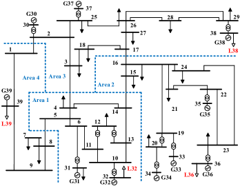
Figure 1: The New England 39-bus system

The analysis above shows that the controller is robust in terms of uncertain parameter $D_{j}$ and unknown disturbance $w_{j}(t)$. Hence P3 is resolved.

6 Case studies

6.1 System Configuration

To verify the performance of the proposed controller, the New England 39-bus system with 10 generators as shown in Figure 1 is used for test. All simulations are implemented in the commercial power system simulation software PSCAD.

We add four (aggregate) controllable loads to the system by connecting them at buses 32, 36, 38 and 39, respectively. Their initial values are set as $(74.1,\ 52.7,\ 52.7,\ 105.4)$ MW. Then the system is divided into four control areas, as shown in Figure 1. Each area contains a controllable load. The communication graph is undirected and set as $L32\leftrightarrow{}{}L36\leftrightarrow{}{}L38\leftrightarrow{}{}L39\leftrightarrow{}{}L32$. For simplicity, we assume the communication is perfect with no delay or loss.

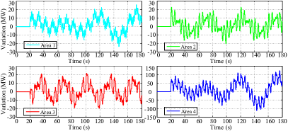
Figure 2: Power variation of renewable resources in each area

In our tests, two cases are studied based on different data: 1) self-generated data in PSCAD; 2) the real data of an offshore wind farm. The variation in the first case is faster than the latter. Parameters used in the controller (11) are given in Table 1.

Table 1: Parameters used in the controller (11)

Area $i$	1	2	3	4
$\beta$	1	0.8	0.8	0.4
$d$	1000	1000	1000	1000
$D$	50	50	50	80
$\gamma$	1	1	1	1
$k_{\alpha}$	10	10	10	10

The value of $B_{ij}$ is given in Table 2.

Table 2: Parameters used in the controller (11)

Line	(1, 2)	(1, 3)	(1, 4)	(2, 3)	(2, 4)
$B_{ij}$	46	47	89	112	24

The $R_{j}$ used in (11) for each area is $R_{j}=[1,6,15,20,15,6,1]$. The corresponding polynomial is $(x+1)^{6}$, where all the roots are $-1$, satisfying the requirement.

6.2 Self-generated data

In the first case, the varying power in each area is shown in Figure 2. Note that the functions of the four curves in Figure 2 are unknown to the controllers. In the controller design, we choose $s_{j}=3$ in (3). Note that this does not mean the actual power variation (curves in Figure 2) are superposition of only three sinusoidal functions.

In this subsection, $\overline{P}_{j}^{in}$ in each area are $(15,\ 15,\ 15,\ 15)$ MW, which are the prediction of aggregated load. It should be pointed out that the prediction is not accurate. The offset errors are $(1,\ 1,\ 1,\ 5)$ MW, which are relatively small but unknown. We compare the performances using controller (10) and (11). Both the two controllers are applied at $t=20$s. The system frequencies are compared in Figure 3.

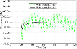
Figure 3: System frequencies under two controls

The green line stands for the frequency dynamics using (10). The frequency oscillation is fierce and nadir is quite low. The black line stands for frequency dynamics using (11). In this situation, the nominal frequency is recovered fast without oscillation. The frequency nadir is much higher than that using (10). This result confirms that our controller can still work well when $\overline{P}_{j}^{in}\neq 0$.

The dynamics of $\mu_{j}$ are given in the left part of Figure 4. The green line stands for $\mu_{j}$ using (10), while the black line stands for that using (11). $\mu_{j}$ of each area converges to a same value, which implies the optimality is achieved, i.e., $\overline{P}_{j}^{in}$ is balanced economically.

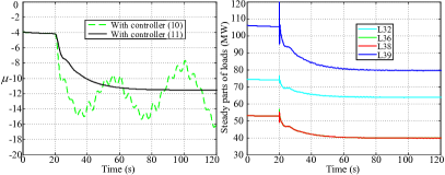
Figure 4: Dynamics of $\mu$ and steady parts of controllable loads

In this scenario, the controllable load in each area is also composed of two parts: a steady part to balance $\overline{P}_{j}^{in}$ and a variation part to mitigate the effects of $\tilde{q}_{j}(t)$. The steady part of controllable load is given in the right part of Figure 4. The controllable loads in the steady state are $(63.8,\ 39.8,\ 39.8,\ 79.6)$ MW. The result is the same as that obtained using CVX to solve the optimization counterpart (i.e., OLC problem (9)).

To demonstrate it more clearly, we define an error index $Err_{j}$ as below.

$$Err_{j}:=\frac{\int_{t_{0}}^{t_{1}}\sqrt{\left(\tilde{A}_{j}(\hat{\alpha}_{j}){\zeta}_{j}-\tilde{q}_{j}(t)\right)^{2}}\text{d}t}{\int_{t_{0}}^{t_{1}}\sqrt{\left(\tilde{q}_{j}(t)\right)^{2}}\text{d}t}$$ (100)

The performance of controllable load tracking power variation in each area is given in Figure 5. We can find that the controllable loads coincide to the power variations with high accuracy. Again, the error index $Err_{j}$ with $t_{0}=20$ and $t_{1}=120$ in this situation are $(0.0084,\ 0.0026,\ 0.0057,\ 0.0019)$, which are also very small.

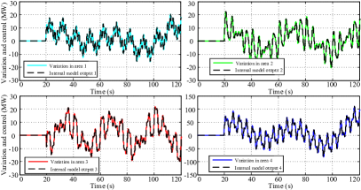
Figure 5: Variation and internal model output with load increases

6.3 Performance under Unknown Disturbances

To test the performance of our controller under high-frequency unknown disturbances, we add random noise $\tilde{w}(t)$ on $\tilde{q}(t)$ into the testing system, which takes the form of $\tilde{w}(t)=[20,20,20,100]\times\text{rand}(t)\ \text{MW}$ , with rand(t) as a function generating a random number between $[0,\ 1]$ at time $t$. In the simulation, a random number is generated every 0.01s. The load control command and the power variations are given Figure 6. As the frequency of external disturbance is quite high, the internal model control is not able to follow it accurately. As a consequence, there exist obvious tracking errors. The system frequency is shown in Figure 7. The inset zooms into the frequency dynamics between 140s-160s, when the system converges to the steady state. The maximal frequency deviation is smaller than 0.003Hz, demonstrating that the unknown disturbance is well attenuated by the proposed controller.

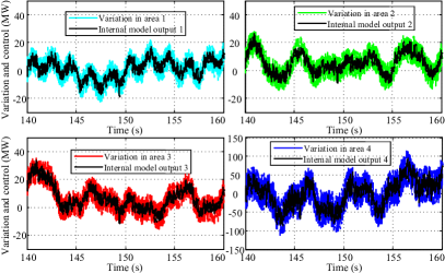
Figure 6: Variation and internal model output with noise

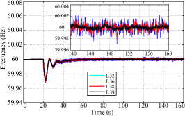
Figure 7: Frequency under external noise

6.4 Simulation with Real Data

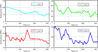
Figure 8: Wind power in each area

In this subsection, we use 300s data points for each area (one data point per second) to illustrate the effectiveness of our controller, which come from a real offshore wind farm. The data is available via the link Wang (2018). Due to agreement with the data provider, its is for personal use only. The wind power in each area is shown in Figure 8, which is added in the simulation at $t=10$s. The power prediction in each area, i.e. $\overline{P}_{j}^{in}$, is $(72,60,49,120)$MW respectively. The frequency dynamics using controller (10) and (11) with the real data are given in Figure 9. Similar to that in Figure 3, the frequency under the controller (10) varies and cannot be restored to the nominal value due to the variation of wind power. On the contrary, the frequency is very smooth when controller (11) is used. The performance of controllable load tracking wind power variation in each area is given in Figure 10. We can find that the controllable loads still coincide with the variations with high accuracy under the proposed controller.

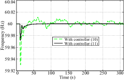
Figure 9: Frequency dynamics with real data

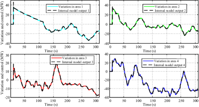
Figure 10: Variation and internal model output with real wind data

6.5 Comparison with Existing Control Methods

First, we compare the proposed method (11) with conventional PI control. In the PI control, the control command is $P_{j}^{l}=K_{P}\omega_{j}+K_{I}\int\omega_{j}\ dt$, where $K_{P}$ in each area are $(500,500,500,800)$, and $K_{I}$ are $(2500,2500,2500,4000)$. The frequency dynamics are given in the left part of Figure 11, where the inset is the enlarged version. It is shown that the frequency nadir is much larger than our method and the variation cannot be eliminated. This result demonstrates the superiority of the proposed method to the traditional PI control.

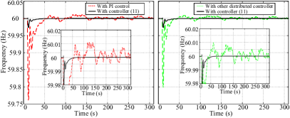
Figure 11: Frequency dynamics compared with PI control (left) and other distributed controller (right)

We also compare the proposed method (11) with the distributed controller in Mallada et al. (2017). To make a valid comparison, we do not consider line constraints when using controller in Mallada et al. (2017), and the objective function is same with this paper. The frequency dynamics are given in the right part of Figure 11. Similarly, the frequency variation is not eliminated, demonstrating the superiority of our controller in coping with unknown and time-varying power imbalance.

7 Conclusion

In this paper, we have addressed the distributed frequency control problem of power systems in the presence of unknown and time-varying power imbalance. We have decomposed power imbalance into three parts at different timescales: the known steady part, the unknown low-frequency variation and the unknown high-frequency residual. Then the distributed frequency control problem at the three different timescales are solved in a unified control framework composed of three timescales:

1. The slow timescale: designing a consensus-based distributed control to allocate the steady part of power imbalance economically;

2. The medium timescale: devising an internal model control to accurately track and compensate for the time-varying unknown power imbalance locally;

3. The fast timescale: using the $L_{2}$-gain inequality to show the robustness of the controller against uncertain disturbances and parameters.

We have conducted numerical experiments using data of the New England system and real-world wind farms. The empirical results show that our distributed controller can mitigate the frequency fluctuation caused by the integration of large uncertain and time-varying renewable generation. The test results also confirm that our controller outperforms existing ones.

This paper intends to provide a systematic approach to deal with unknown and time-varying power imbalance in an economic manner. Besides renewable generations, power oscillations and malicious attacks on controllers can also lead to unknown and time-varying power variation in power system operation. The proposed method could be extended to cope with such problems, which are among our future studies.

References

References

• Aguirre et al. (2008) Aguirre, L.A., Rodrigues, D.D., Lima, S.T., Martinez, C.B., 2008. Dynamical prediction and pattern mapping in short-term load forecasting. Int. J. Electr. Power Energy Syst. 30, 73 – 82.
• Ahmadi-Khatir et al. (2013) Ahmadi-Khatir, A., Bozorg, M., Cherkaoui, R., 2013. Probabilistic spinning reserve provision model in multi-control zone power system. IEEE Trans. Power Syst. 28, 2819–2829.
• Barooah et al. (2015) Barooah, P., Buic, A., Meyn, S., 2015. Spectral decomposition of demand-side flexibility for reliable ancillary services in a smart grid, in: System Sciences (HICSS), 2015 48th Hawaii International Conference on, IEEE. pp. 2700–2709.
• Bušiā and Meyn (2016) Bušiā, A., Meyn, S., 2016. Distributed randomized control for demand dispatch, in: Decision and Control (CDC), 2016 IEEE 55th Conference on, IEEE. pp. 6964–6971.
• Cai et al. (2017) Cai, D., Mallada, E., Wierman, A., 2017. Distributed optimization decomposition for joint economic dispatch and frequency regulation. IEEE Transactions on Power Systems 32, 4370–4385.
• Dörfler et al. (2016) Dörfler, F., Simpson-Porco, J.W., Bullo, F., 2016. Breaking the hierarchy: Distributed control and economic optimality in microgrids. IEEE Trans. Control Network Syst. 3, 241–253.
• Jokić et al. (2009) Jokić, A., Lazar, M., van den Bosch, P.P., 2009. Real-time control of power systems using nodal prices. Int. J. Elect. Power Energy Syst. 31, 522–530.
• Kasis et al. (2017) Kasis, A., Devane, E., Spanias, C., Lestas, I., 2017. Primary frequency regulation with load-side participation part i: Stability and optimality. IEEE Transactions on Power Systems 32, 3505–3518.
• Khalil (1996) Khalil, H.K., 1996. Nonlinear systems. volume 3. Prentice hall New Jersey.
• Kundur (1994) Kundur, P., 1994. Power System Stability and Control. volume 7. McGraw-hill New York.
• Li et al. (2016) Li, N., Zhao, C., Chen, L., 2016. Connecting automatic generation control and economic dispatch from an optimization view. IEEE Trans. Control Network Syst. 3, 254–264.
• Lu et al. (2016) Lu, L.Y., Liu, H.J., Zhu, H., 2016. Distributed secondary control for isolated microgrids under malicious attacks, in: 2016 North American Power Symposium (NAPS), pp. 1–6.
• Mallada et al. (2017) Mallada, E., Zhao, C., Low, S., 2017. Optimal load-side control for frequency regulation in smart grids. IEEE Transactions on Automatic Control 62, 6294–6309.
• Milan et al. (2013) Milan, P., Wächter, M., Peinke, J., 2013. Turbulent character of wind energy. Phys. Rev. Lett. 110, 138701.
• Min and Abur (2006) Min, L., Abur, A., 2006. Total transfer capability computation for multi-area power systems. IEEE Trans. Power Syst. 21, 1141–1147.
• Obregon-Pulido et al. (2002) Obregon-Pulido, G., Castillo-Toledo, B., Loukianov, A., 2002. A globally convergent estimator for n-frequencies. IEEE Trans. Automat. Contr. 47, 857–863.
• Qin et al. (2018) Qin, B., Zhang, X., Ma, J., Deng, S., Mei, S., Hill, D.J., 2018. Input-to-state stability based control of doubly fed wind generator. IEEE Transactions on Power Systems 33, 2949–2961.
• Schweppe et al. (1980) Schweppe, F.C., Tabors, R.D., Kirtley, J.L., Outhred, H.R., Pickel, F.H., Cox, A.J., 1980. Homeostatic utility control. IEEE Trans. Power Apparatus Syst. PAS-99, 1151–1163.
• Stegink et al. (2017) Stegink, T., De Persis, C., van der Schaft, A., 2017. A unifying energy-based approach to stability of power grids with market dynamics. IEEE Trans. Autom. Control 62, 2612–2622.
• Trip et al. (2016) Trip, S., Bürger, M., De Persis, C., 2016. An internal model approach to (optimal) frequency regulation in power grids with time-varying voltages. Automatica 64, 240–253.
• Wang et al. (2017a) Wang, X., Hong, Y., Yi, P., Ji, H., Kang, Y., 2017a. Distributed optimization design of continuous-time multiagent systems with unknown-frequency disturbances. IEEE Trans. Cybern. 47, 2058–2066.
• Wang (2018) Wang, Z., 2018. Wind power in each area. https://drive.google.com/drive/folders/1vFXvVp3-mLocxlW4jRXMnhcodOCD8S4q.
• Wang et al. (2017b) Wang, Z., Liu, F., Low, S.H., Zhao, C., Mei, S., 2017b. Distributed frequency control with operational constraints, part i: Per-node power balance. IEEE Trans. Smart Grid, in press .
• Wang et al. (2017c) Wang, Z., Liu, F., Low, S.H., Zhao, C., Mei, S., 2017c. Distributed frequency control with operational constraints, part ii: Network power balance. IEEE Trans. Smart Grid, in press .
• Wang et al. (2018) Wang, Z., Liu, F., Pang, J.Z., Low, S., Mei, S., 2018. Distributed optimal frequency control considering a nonlinear network-preserving model. IEEE Transactions on Power Systems, in press .
• Weitenberg et al. (2017) Weitenberg, E., Jiang, Y., Zhao, C., Mallada, E., De Persis, C., Dörfler, F., 2017. Robust decentralized secondary frequency control in power systems: Merits and trade-offs. arXiv preprint arXiv:1711.07332 .
• Xi et al. (2017) Xi, K., Lin, H.X., van Schuppen, J.H., 2017. Power-imbalance allocation control of power systems – a frequency bound for time-varying loads, in: 2017 36th Chinese Control Conference (CCC), pp. 10528–10533.
• Xu et al. (2016) Xu, D., Wang, X., Chen, Z., 2016. Output regulation of nonlinear output feedback systems with exponential parameter convergence. Syst. Control Lett. 88, 81 – 90.
• Zhang and Papachristodoulou (2015) Zhang, X., Papachristodoulou, A., 2015. A real-time control framework for smart power networks: Design methodology and stability. Automatica 58, 43–50.
• Zhao et al. (2014) Zhao, C., Topcu, U., Li, N., H.Low., S., 2014. Design and stability of load-side primary frequency control in power systems. IEEE Trans. Autom. Control 59, 1177–1189.
• Zhou et al. (1996) Zhou, K., Doyle, J.C., Glover, K., 1996. Robust and optimal control. volume 40. Prentice hall New Jersey.